Matrix model for deconfinement in a gauge theory in dimensions
Abstract
We use an effective matrix model to study deconfinement in a pure gauge theory, without quarks, in dimensions. Expanding about a constant background field we construct an effective potential for the eigenvalues of the thermal Wilson line for general and in the large- limit. The numerical results are presented using one, two, and four free parameters, which are determined by fitting directly to the lattice data for the pressure. The matrix model shows a good agreement with numerical lattice simulations for the pressure and the interaction measure, starting from the perturbative limit up to the critical temperature. For the pressure, the details of -dependent nonperturbative terms are relevant only in a narrow transition region below . This is also the range where the Polyakov loop deviates notably from one. In accordance with the lattice results we find that, up to a trivial factor , there is only a mild dependence on the number of colors.
I Motivation
Nowadays increasing attention is being devoted to the study of the deconfinement phase transition in QCD. There are different, complementary approaches to the underlying physics, which is strictly nonperturbative: numerical simulations on the lattice, the construction of various effective theories, and lastly, results from the collisions of heavy ions at ultrarelativistic energies. In this work we investigate the key aspects of deconfinement by using an effective matrix model for three-dimensional pure gauge theories.
The matrix model respects the center symmetry of the underlying pure glue theory. It is valid over a wide temperature range, starting from the perturbative limit up to the critical temperature for deconfinement . The degrees of freedom are given by the eigenvalues of the thermal Wilson line, and the parameters of the model are obtained by fitting the pressure as computed within lattice QCD in Ref. Caselle et al. (2011a).
It is known that in pure gauge theory the Polyakov loop approaches unity in the perturbative limit, and vanishes below the deconfining temperature . This behavior can be modeled by constructing an effective theory for the eigenvalues of the thermal Wilson line. Assuming a constant background field for the timelike component of the gluonic vector potential, one first computes the perturbative potential. In order to drive the transition to confinement, one then constructs additional -dependent and -independent nonperturbative contributions. This is a reasonable approach provided that the expectation value of the Polyakov loop is dominated by the classical configuration for the background field, and not by quantum fluctuations around . This assumption is certainly valid for an infinite number of colors, where represents a master field for deconfinement Gopakumar and Gross (1995). Namely, in the large- limit, the vacuum is dominated by a single master field at any temperature, since quantum fluctuations are typically suppressed by powers of . Nevertheless, we find that this approach works reasonably well even for two colors, both in Dumitru et al. (2011, 2012), and in , see Ref. Bicudo et al. (2013).
A more complete model for deconfinement should ideally consider gauge theories coupled to light quarks in space-time dimensions. However, lattice results provide convincing evidence that the QCD transition is mainly driven by the dynamics of gluons which are the dominant degrees of freedom in the deconfined phase Karsch (2002). Moreover, gauge theories in three and four space-time dimensions are closely related and share many important features, like asymptotic freedom, and a confinement-deconfinement phase transition at a critical temperature Teper (1999); Johnson and Teper (2002); Meyer and Teper (2003). For these reasons, three-dimensional pure glue theories are widely used both on the lattice and in effective theories, in order to obtain a better understanding of the QCD transition from a broader perspective, see e.g. Refs. Teper (1999); Johnson and Teper (2002); Lucini and Teper (2002); Meyer and Teper (2003); Bursa and Teper (2006); Bialas et al. (2009); Liddle and Teper (2008); Caselle et al. (2011b); Bialas et al. (2012).
An important question is the dependence of thermodynamic properties on the number of colors. In this sense, the large- limit is of particular importance, since it serves as a suitable basis for various effective approaches to QCD, see e.g. Ref. Moshe and Zinn-Justin (2003) and refs. therein for a detailed discussion. Matrix models, for instance, are motivated by general expectations that in the large- limit all correlation functions of gauge-invariant operators factorize, and consequently the functional integral is dominated by a single master gauge field Gopakumar and Gross (1995).
Recent lattice simulations of pure gauge theories at nonzero temperature indicate that, except for a trivial proportionality to the number of gluons , the thermodynamic observables in are essentially independent of , and that is already sufficiently close to the large- limit Boyd et al. (1996); Lucini and Teper (2001); Teper (2002); Umeda et al. (2009); Borsanyi et al. (2011, 2012); Lucini and Panero (2012). This observation is of particular importance, because it supports the validity of analytical techniques and effective theories based on large- approximations.
In , the matrix model has been extensively studied for various groups and also in the large- limit Pisarski (2000); Meisinger et al. (2002); Meisinger and Ogilvie (2002); Dumitru et al. (2004); Oswald and Pisarski (2006); Pisarski (2006, 2007); Hidaka and Pisarski (2008, 2009a, 2009b, 2010); Dumitru et al. (2011, 2012); Pisarski and Skokov (2012); Kashiwa et al. ; Sasaki and Redlich (2012); Ruggieri et al. (2012); Diakonov et al. (2012); Ogilvie (2012); Kashiwa and Pisarski (2013); Lin et al. (2013), showing that one- and two- parameter models provide an overall good agreement with the lattice data for the pressure and interaction measure. In Ref. Bicudo et al. (2013) we applied the matrix model to study deconfinement in three-dimensional pure gauge theory for the special case . As in four dimensions, we find that the model works reasonably well even for two colors. Similar to , we demonstrated that in three-dimensional theory, for the pressure the details of the matrix model become relevant only in a narrow transition region, from to . This is also the range where the Polyakov loop notably deviates from one. The ’t Hooft loop, on the other contrary, is sensitive to the details of the model in a much wider region, up to .
In this work we extend the study of Ref. Bicudo et al. (2013) to general groups in . The thermodynamics of three-dimensional pure glue theories was studied on the lattice by many authors, see e.g. Refs. Bialas et al. (2000, 2005, 2009); Liddle and Teper (2008); Bialas et al. (2010); Caselle et al. (2011b, a); Bialas et al. (2012); Lucini and Panero (2012). An important observation is that in the behavior of thermodynamical quantities, like pressure , energy density , and interaction measure , looks similar to that in four dimensions. As in , lattice results show that in three dimensions there is only a small dependence on the number of colors Lucini and Teper (2002).
Remarkably, in three dimensions, the value for the interaction measure scaled by and divided by the number of gluons, , assumes approximately the same constant value on the lattice for for all Caselle et al. (2011a),
| (1) |
To a good approximation, this implies that, except for a narrow region near the phase transition, , the pressure divided by , is dominated by a constant term times ,
| (2) |
Similar lattice results are obtained in four dimensions, where for .
In lattice calculations can be performed with a great precision, keeping artifacts well under control. Therefore, comparing our results to the lattice data will provide a crucial test for the validity of the matrix model.
This paper is organized as follows: in Sec. II we construct the confining and deconfining vacua in the presence of a constant background field. In Sec. III we derive the effective potential in for an gauge group as a sum of a perturbative and a nonperturbative part. In Sec. IV we present the analytical and numerical solution for the potential for general and in the large- limit using a so-called uniform eigenvalue ansatz. In Sec. V we show the pressure, the interaction measure, and the Polyakov loop for , and compare to the recent lattice data of Ref. Caselle et al. (2011a). In Sec. VI we address the question of possible metastable solutions in the perturbative potential. Conclusions and outlook are given in Sec. VII.
II The confined and deconfined vacua
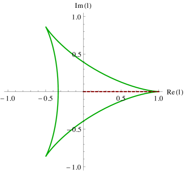
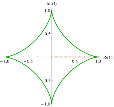
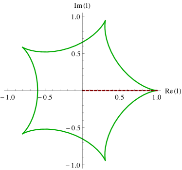
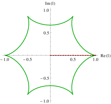
In the absence of dynamical quarks, the pure gauge theory exhibits a deconfinement phase transition at a critical temperature related to the breaking of the center symmetry of the gauge group. The appropriate gauge-invariant order parameter for this transition is given by the Polyakov loop , defined as the trace of the thermal Wilson line ,
| (3) |
where
| (4) |
In the deconfined phase, , the allowed vacua of the pure gauge theory exhibit an -fold degeneracy, where the thermal expectation value of the Polyakov loop is given by one of the th roots of unity,
| (5) |
These vacuum states are degenerate and can be transformed into each other by global rotations,
| (6) |
Consequently, when choosing one particular state, the center symmetry is spontaneously broken. Defining the Polyakov loop to be real, which is always possible by global transformations, the expectation value of the order parameter approaches unity in the perturbative vacuum, as .
In the confined phase, , the center symmetry is restored, and the expectation value of the Polyakov loop vanishes, . This behavior of the order parameter is also confirmed by lattice-QCD calculations, where the expectation value of the renormalized Polyakov loop is zero in the confined and nonzero in the deconfined phase, approaching unity in the perturbative limit.
In general, the Polyakov loop is a complex-valued quantity. Only for the special case the order parameter is real, assuming values between and . In Fig. 1 we plot the boundaries of for different numbers of colors. Depending on the parametrization of , which is an element of the Lie algebra of the gauge group, the Polyakov loop takes certain values within the solid lines. The degenerate ground states in the deconfined phase reside at the corners, while the confining vacuum corresponds to the origin of the diagrams. It is obtained by computing the average of the deconfined vacua,
| (7) |
and is therefore automatically invariant under transformations.
In this paper the numerical results are obtained using a uniform eigenvalue ansatz Dumitru et al. (2012). Within this ansatz, is parameterized in such a way that the Polyakov loop always assumes values along the real axis in Fig. 1.
II.1 Background field
Given the known behavior of the Polyakov loop, we can model the phase transition and the deconfined phase, , by constructing an effective theory for the eigenvalues of the thermal Wilson line. The simplest ansatz is to assume a constant, but nonzero value for the time component of the vector potential. Due to gauge transformations, it is always possible to write the background field as
| (8) |
where is a traceless diagonal matrix in the Lie algebra. The eigenvalues are constrained only by the unimodularity,
| (9) |
and the number of independent ’s corresponds to the rank of the group,.
In the presence of the background field (8), the Wilson line is given by a diagonal matrix,
| (10) | ||||
The Polyakov loop is the trace over the Wilson line,
| (11) |
II.1.1 Perturbative vacuum
The degenerate ground states (5) in the deconfined phase can be described by an appropriate choice for the matrix ,
| (12) | ||||
where are traceless diagonal matrices of the form
| (13) |
with entries , and entries . The are also referred to as hypercharges Dumitru et al. (2012), and serve as generators for the elements of the center of the gauge group,
| (14) |
where is an unit matrix. Thus, under global rotations the hypercharges are transformed into each other,
| (15) |
The perturbative vacuum where the Polyakov loop is equal to one, , is obtained for
| (16) |
II.1.2 Confining vacuum
In the confining vacuum , the Polyakov loop must vanish, . The confining vacuum is constructed as the average of all degenerate ground states (13),
| (17) | ||||
| (22) |
and is therefore is automatically invariant. The eigenvalues of are separated by a constant spacing,
| (23) |
This implies that the eigenvalues of the Wilson line,
| (24) |
are equally distributed about the unit circle, with a spacing . Thus, the confining vacuum is characterized by a uniform, i.e., complete repulsion of eigenvalues.
III The Potential
Provided that the expectation value of the Polyakov loop near the critical temperature is dominated by the classical configuration of the background field (8), we can model the deconfinement phase transition by introducing a potential for . In this section we construct the effective potential as a sum of two parts: the perturbative potential, , and nonperturbative contributions
III.1 Parametrization of the generators
Before proceeding, we need to introduce a suitable parametrization for the generators of the Lie algebra. It is convenient to choose the same basis as in Ref. Bhattacharya et al. (1992) comprised of diagonal matrices, and off-diagonal matrices.
III.2 Perturbative potential
The perturbative potential is computed by expanding about the classical background field (8), see e.g. Refs. Bhattacharya et al. (1991, 1992); Korthals Altes et al. (1997); Dumitru et al. (2012). To one-loop order in , the result is given by
| (29) |
see Ref. Korthals Altes et al. (1997), where is the covariant derivative in the adjoint representation in the presence of the background field,
| (30) | ||||
and is the gauge-covariant d’Alembertian,
| (31) |
The trace in Eq. (29) is over all momenta and color degrees of freedom. In order to evaluate the color trace, one has to sum over all commutators between and the generators of the Lie algebra defined in Eqs. (25) and (26). This can be done using the normalizations in Eqs. (27) and (28).
Since is a diagonal matrix, it commutes with all diagonal generators,
| (32) |
Thus, for each degree of freedom along diagonal generators the potential is as in zero background field, i.e., it has no -dependence,
| (33) |
where is the two-dimensional vector in momentum space, and is the Matsubara frequency for bosonic fields.
For all off-diagonal generators the commutator with is nonzero,
| (34) |
where we introduced the notation
| (35) |
Therefore, the propagators for the degrees of freedom along the ladder operators are as in zero background field, except that is shifted by a constant amount to
| (36) |
Summing over all generators, the full perturbative potential to one-loop order is
| (37) |
The first term in Eq. (37) is from diagonal modes , while the second term comes from the off-diagonal modes . As demonstrated in Ref. Bicudo et al. (2013), the sum integrals in Eq. (37) can be evaluated via contour integration Gross et al. (1981),
| (38) | ||||
| (39) |
where we used the polylogarithm function,
| (40) |
and the Riemann zeta function,
| (41) |
The final result for the one-loop perturbative potential is then given by
| (42) |
where .
The result for , Eq. (42), can also be written as a sum of the zero-field contribution, independent of ,
| (43) |
and the quantum correction,
| (44) | ||||
Note that the quantum correction is automatically zero in the perturbative vacuum . The zero-field contribution (43) corresponds to the free energy of an ideal gas of massless gluons.
III.3 Nonperturbative potential
In order to model the deconfinement phase transition at it is necessary to add nonperturbative terms to the perturbative potential. In general, the nonperturbative contributions may include similar functions of to the ones found at one-loop order.
III.3.1 -independent term
Since the lattice data for is constant in the region Bialas et al. (2009); Caselle et al. (2011a) for all , see Eq. (1), we must certainly include a nonperturbative term which is independent of ,
| (45) |
similar to the free energy of an ideal gas of massless gluons in Eq. (43).
Notably, in dimensions the one-loop perturbative corrections to the pressure are D’Hoker (1981, 1982a, 1982b), and so automatically proportional to , because in three dimensions has the dimension of mass. The results of numerical simulations on the lattice are nevertheless surprising, since it is not natural to expect that perturbation theory at one-loop order is dominant down to temperatures as low as . Moreover, on the lattice there is no evidence of higher-order perturbative contributions. The two-loop order terms would be , while the three-loop order contributions are independent of temperature, . In detail, perturbation theory is more involved, including logarithms of D’Hoker (1981, 1982a, 1982b).
III.3.2 -dependent term
III.3.3 Vandermonde determinant
Finally, in order to avoid another phase transition above , we need to add a Vandermonde-like term to the potential, see Ref. Bicudo et al. (2013). It is interesting to note that in our matrix model a Vandermonde term can be introduced using different approaches.
Leading order in a mass expansion
One possibility is to consider a mass parameter in the gluon propagator, and then to expand the one-loop determinant (29) to leading order in the mass Bicudo et al. (2013),
| (47) |
The first term in the expansion reproduces the one-loop order perturbative potential, while the second term corresponds to the Vandermonde determinant.
The trace over momentum in Eq. (47) can be evaluated via contour integration,
| (48) | ||||
| (49) |
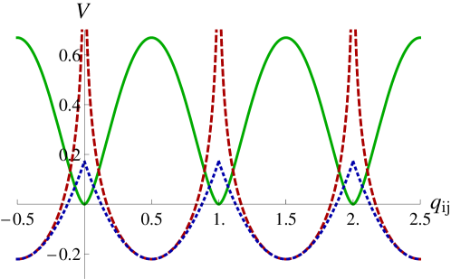
The function is divergent at and has a minimum at , see Fig. 2. Moreover, due to the symmetry, is periodic in , see Sec. III.5. Identifying the mass parameter with the Debye screening mass , in three dimensions see e.g. Refs. Kajantie et al. (1997); Rischke (2004). Thus, the overall temperature dependence of the Vandermonde term is ,
| (50) |
where acts just as a mass parameter.
Two-loop quantum correction
Performing a mass expansion is just one possibility to derive the Vandermonde determinant. The same term can also be found at two-loop order which may already include nonperturbative contributions. From perturbative calculations in four dimensions Bhattacharya et al. (1992); Belyaev and Eletsky (1990); Enqvist and Kajantie (1990), we know that the two-loop corrections to the potential in a constant background field (8) include terms similar to the ones obtained at one-loop order, as well as terms similar to the second derivative of the one-loop result with respect to .
Similar arguments should apply in . Thus we derive
| (51) |
This result is identical to the Vandermonde term obtained via the mass expansion, Eq. (48).
III.3.4 Linear term
In order to derive a regularized version of the Vandermonde term, we expand the function around its minimum at , keeping only terms up to order ,
| (52) |
where returns the decimal part of . This ensures that the periodicity in is maintained, see Fig. 2. We refer to this term as linear, since it gives a contribution linear in for small when expanding around the minimum. Including the temperature dependence and the sum, the linear nonperturbative term is
| (53) | ||||
Adjoint Higgs phase
The need for a Vandermonde or a linear contribution to the potential is the following: for static fields, couples to the spatial degrees of freedom as an adjoint scalar. When , and consequently , develops a nonvanishing expectation value, the system is in an adjoint Higgs phase Pisarski (2006); Unsal and Yaffe (2008). While there is no gauge-invariant order parameter for an adjoint Higgs phase, there can still be a first-order transition from a truly perturbative phase, where , to one where . This scenario would correspond to a second phase transition, at a temperature higher than . Though possible, lattice calculations find no evidence of such a second phase transition.
This can be avoided by adding a Vandermonde or a linear term to the effective potential, which will generate a nonzero expectation value for at any temperature, obviating such a second phase transition. As a consequence, the theory is in an adjoint Higgs phase for all . In practice, however, for the parameters of the model determined by fitting the lattice data, the condensate is very small except near the critical temperature , see Sec. V.
III.3.5 Full nonperturbative potential
Summing all contributions, the nonperturbative potential with the Vandermonde determinant (48) takes the form
| (54) |
where we introduced three parameters which will be determined in Sec. IV.7. For the linear term (53) the full nonperturbative potential is obtained by replacing in Eq. (54) the term as
| (55) |
III.4 Effective Potential
III.5 symmetry
The effective potential (57) is a function of , where are the eigenvalues of the thermal Wilson line (10). They are the fundamental variables of the matrix model. While the Wilson line is gauge variant, its eigenvalues are gauge invariant.
Applying a global transformation to the Wilson line, ,
| (59) |
the eigenvalues undergo a uniform rotation along the unit circle by a constant angle ,
| (60) |
Due to the periodicity in , it is sufficient to restrict the eigenvalues of the matrix to lie in the interval Thus, the transformation (60) is associated with a constant shift of the matrix elements ,
| (61) |
This implies that the differences either vanish or equal leaving invariant,
| (62) |
Therefore, our effective potential is manifestly symmetric and periodic in . Note that in the confining vacuum the transformation corresponds to cyclic permutations of the eigenvalues of the Wilson line (24) and of the matrix (63).
IV Uniform eigenvalue ansatz
In this section we present the numerical and analytical solution for the potential using a uniform eigenvalue Ansatz Dumitru et al. (2012), which guarantees that the Polyakov loop is always real.
We are interested in studying the region between the perturbative and confining vacuum, , indicated by the dashed lines in Fig. 1. In this case, a suitable parametrization of the matrix is given by a straight line from to (17),
| (63) |
where is a diagonal matrix with the eigenvalues
| (64) |
For an even number of colors, there are pairs of eigenvalues, , , where . For odd , there are again pairs of eigenvalues, , where , and the remaining eigenvalue is zero. All ’s have the constant spacing
| (65) |
The eigenvalues of the associated Wilson line are distributed about the unit circle, with a spacing ,
| (66) |
In the large- limit, this ansatz generates a uniform eigenvalue density , where , see Sec. IV.3.
We stress that in dimensions the uniform eigenvalue Ansatz applies for two or three colors, but is not an exact solution for four or more colors, see Ref. Dumitru et al. (2012). It is, however, rather close to the exact numerical solution. For to in dimensions, for instance, the difference between the uniform eigenvalue Ansatz and the exact solution is less than for all thermodynamic quantities and for the expectation value of the Polyakov loop, even at where the differences are naturally greatest. This is our main motivation to employ the uniform Ansatz. A general parametrization of the background field is discussed in Sec. VI.
IV.1 Polyakov loop
Taking the trace of the Wilson line (66) gives the Polyakov loop for even ,
| (67) | ||||
and for odd ,
| (68) | ||||
where we used Eq. (64) for . The perturbative vacuum, is realized for , while the confining vacuum, is at .
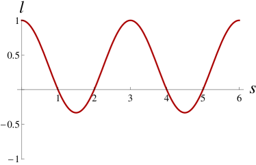
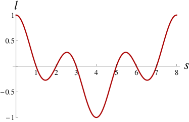
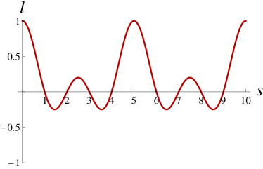
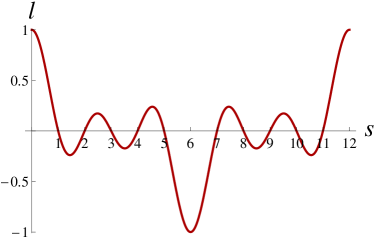
In Fig. 3 we plot the Polyakov loop in the uniform eigenvalue ansatz as a function of for different numbers of colors. The function is periodic in and symmetric around , and . For any the Polyakov loop takes values along the real axis within the solid lines in Fig. 1, and thus represents a possible physical solution.
IV.2 The Potential
IV.2.1 Perturbative and nonperturbative potential
In the uniform eigenvalue ansatz (64), the potential becomes a function of through the dependence of on ,
| (69) |
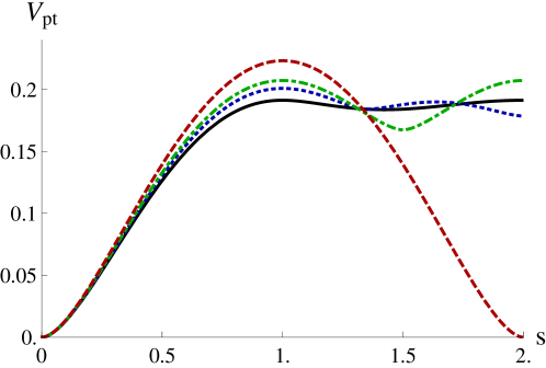
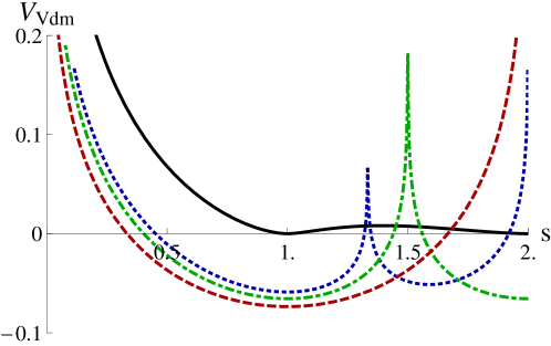
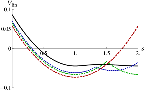
In Figs. 4, 5, and 6 we plot the perturbative potential (42), the Vandermonde term (48), and the linear term (53) for different numbers of colors in the region between the perturbative vacuum, and the confining vacuum, . The perturbative potential exhibits a minimum at and a maximum at , while the nonperturbative terms both have a minimum at the confining vacuum .
We note that the Vandermonde term is divergent for . However, in the presence of a Vandermonde or a linear term the condensate for never identically vanishes. A nonzero condensate for will also ensure that the thermodynamical quantities computed at the minimum of the effective potential remain finite.
IV.2.2 Effective potential
Before we discuss the effective potential, it is useful to make some remarks on the summation over the eigenvalues . The perturbative and nonperturbative terms in Eqs. (42), (54), and (55) are even functions in of the form
| (70) |
In the uniform eigenvalue Ansatz, Eq. (69), this sum can be written as a function of the parameter
| (71) |
It is convenient to decompose the effective potential into two parts,
| (72) |
where denotes the -dependent terms.
Using Eq. (71), in the presence of the Vandermonde determinant we derive
| (73) |
where
| (74) |
is a temperature-dependent parameter.
For the linear nonperturbative term (53), in the relevant region between and , the effective potential is obtained by replacing the term in as
| (75) |
IV.3 Large- Limit
In order to study the large- limit, we introduce the variable
| (76) |
Then, the eigenvalues become a function of
| (77) |
and the sum over can be written as an integral over ,
| (78) |
Using this integral, the -dependent part of the effective potential with the Vandermonde term in Eq. (73) takes the form
| (79) | ||||
For the linear nonperturbative term (53), the large- limit of effective potential in the relevant region between and is given by replacing the term in Eq. (79) as
| (80) |
| Vdm | lin | Vdm | lin | |
|---|---|---|---|---|
| 1. | 1. | 2.77259 | 2.77259 | |
| 0.795883 | 0.768018 | 1.84148 | 2.33328 | |
| 0.735259 | 0.704746 | 1.55426 | 2.20086 | |
| 0.707102 | 0.677182 | 1.41634 | 2.14137 | |
| 0.691139 | 0.662458 | 1.33576 | 2.10918 | |
| 0.638659 | 0.628419 | 1.0354 | 2.03424 |
IV.4 The order of the phase transition
Lattice results of Ref. Liddle and Teper (2008) indicate that in dimensions the phase transition is of second order for , of very weak first order for , and of stronger first order for . In our matrix model the phase transition is of second order for , while for the transition is of first order. The reason for the discrepancy between our model and numerical simulations on the lattice is due to infrared fluctuations D’Hoker (1982b) not included in our effective theory, which render the transition second order for three colors in dimensions.
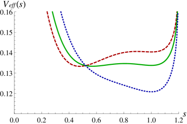
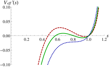
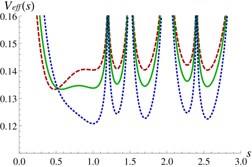
In order to illustrate the behavior of the effective potential (72) near , in Fig. 7 we show , and as a function of for . Depending on the value of the temperature-dependent parameter defined in Eq. (74), we can describe the transition from deconfinement to confinement.
-
(i)
At the system is in the complete QGP phase, with a global minimum at the perturbative vacuum , and a maximum at the confining vacuum .
-
(ii)
In the semi-QGP region, , there is a global minimum at and a second extremum at which corresponds to a second degenerate minimum for , or to a local minimum for .
-
(iii)
At the transition to confinement takes place. For a first-order phase transition, the global minimum jumps at from a critical value to the confining vacuum at
The first-order phase transition becomes stronger with increasing . This is supported by universality class arguments von Smekal et al. (2011); Strodthoff et al. (2010) and numerical simulations on the lattice, where the first order of the transition becomes more pronounced for larger Liddle and Teper (2008). Accordingly, the value for decreases with increasing number of colors, and approaches a constant value in the large- limit,
| (81) |
In Table 1 we list the values for , and for different .
IV.5 The minimum of the effective potential
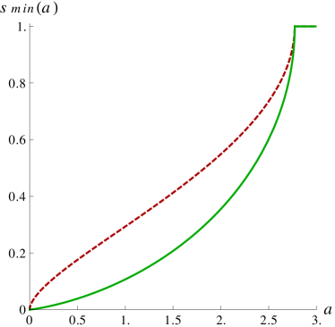
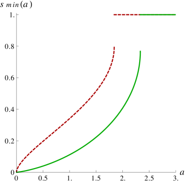
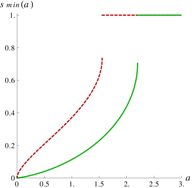
In order to compute the thermodynamic quantities, like pressure and interaction measure, we first have to determine the minimum of the effective potential (72) as a function of the temperature. The minimum is obtained by solving numerically the equation
| (82) |
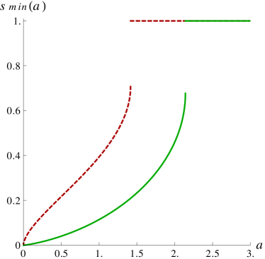
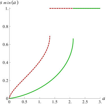
in the region between the perturbative and confining vacuum, . This defines the minimum as a function of the parameter .
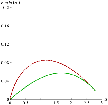
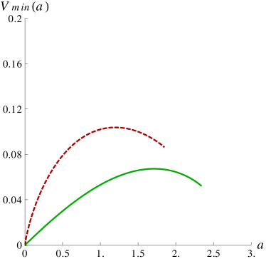
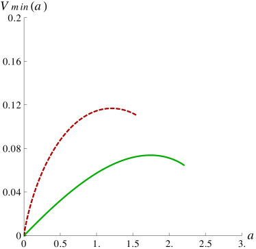
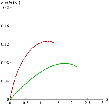
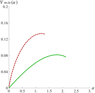
Using the solution for , we can obtain an expression for the potential at the minimum which depends only on
| (83) |
where is given by Eq. (79). This will become useful when we compute the pressure. In Figs. 8, 9, and 10 we plot the solutions for and as a function of for and in the large- limit.
In order to determine the temperature dependence of the minimum, we apply the definition for the parameter in Eq. (74),
| (84) | ||||
| (85) |
IV.6 Pressure and interaction measure
The pressure is defined as minus the effective potential at the minimum,
| (86) |
A more straightforward way to compute the pressure is to use directly the solution for (85),
| (87) |
From the pressure we can derive the interaction measure,
| (88) |
At very high temperatures, the pressure approaches a constant perturbative limit,
| (89) |
while the interaction measure vanishes,
| (90) |
Both the pressure and interaction measure in three-dimensional pure gauge theory were computed on the lattice for in Ref. Caselle et al. (2011a).
IV.6.1 Susceptibility
In order to study the deconfinement temperature , it is also relevant to compute the susceptibility. The common way to determine the critical temperature on the lattice in pure gauge theory is via the susceptibility for the Polyakov loop, which exhibits a peak at . An equivalent method is to look at the susceptibility for the pressure, which may be defined as
| (91) |
This quantity also has a peak at the deconfinement temperature see Fig. 11.
IV.7 Fixing the parameters at

IV.7.1 One-parameter model
The effective potential (72) involves three parameters . Introducing two constraints at the transition temperature leaves only one free parameter, say , which is determined by fitting the lattice data for the pressure of Ref. Caselle et al. (2011a).
-
(i)
The first condition is that the transition occurs at . From Eq. (74) for the temperature-dependent parameter , we then derive as a function of
(92)
In the deconfined phase, the pressure is proportional to the number of gluons, Below the critical temperature, the gluons are confined in colorless glueballs which are exponentially suppressed, , where represents some glueball mass. Thus, in the confined phase the pressure is by a factor smaller than above .
-
(ii)
Therefore, as a second condition we impose that the pressure identically vanishes at the critical temperature,
(93)
Using the equation for the pressure (87), the second condition (93) allows to determine as a function of ,
| (94) |
where the values for and are listed in Table 1. Note that the constraint we impose in Eq. (93) is just an approximation. Ideally, we should fit the pressure to some sort of hadronic, i.e., glueball resonance gas in the confined phase.
IV.7.2 Two-parameter model
The effective potential in Eq. (72) can be generalized to include terms . In the two-parameter model the constants and remain unchanged, while is replaced by a temperature-dependent parameter,
| (95) |
which is equivalent to adding a bag constant to the effective potential. The two-parameter model is the most general case studied nowadays.
IV.7.3 Four-parameter fit
We also study a four-parameter fit by extending the two-parameter model by two additional free parameters: one for the critical temperature , and one for the perturbative limit of the pressure defined in Eq. (89). The parameter for is introduced in order to take into account higher-order loop contributions to the perturbative potential. In addition, the parameter for accounts for possible glueball effects near the transition, which are not included in the matrix model. In our model, we fix the parameters by imposing the constraint that the pressure vanishes at . Ideally, however, we should match the pressure to some hadronic resonance gas below the critical temperature. This gas is made of massive glueballs, and thus can be described by a series of Boltzmann factors. If there are many massive glueballs, as in a Hagedorn spectrum, the temperature dependence of the glueball contribution may become more complicated, including powers of , where is the Hagedorn temperature Hagedorn (1965). The emergence of a Hagedorn-like spectrum (i.e., an exponential growth in the number of hadronic states, as a function of their mass) has been studied in and in a recent work Cohen and Krejcirik (2011).
In the condition provides a good approximation even for two colors Dumitru et al. (2012). In we find that this simplified constraint works well for larger . For small however, we need to relax the condition , because the glueball contribution to the pressure in the confined phase is not negligible.
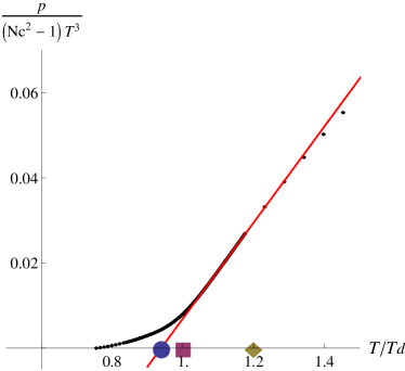
Figure 11 shows the lattice data for the pressure and the corresponding susceptibility , defined in Eq. (91) for . Near the transition at , we find three different temperatures:
-
(i)
First, the critical temperature can be determined from the susceptibility which has a maximum at .
-
(ii)
The inflection point corresponds to the temperature where the derivative of the pressure is maximal. This coincides with the peak of the interaction measure, and with the point at which the susceptibility vanishes.
-
(iii)
The best estimate for the temperature at which the pressure vanishes, is found by the intercept of the tangent to the inflection point of the pressure and the -axis.
For we get for the inflection point, and for the intercept temperature. We find that for small , the critical temperature determined from the lattice data via the susceptibility does not coincide with the estimated value for the intercept temperature , at which the pressure vanishes. This is the main motivation to allow for a shift in introduced in the four-parameter fit. We stress, however, that our four-parameter fit should be regarded just as an approximation to a more complete model including an effective theory for the confined phase.
Note that the beauty and simplicity of these three models including one, two, and four free parameters is that, as a common denominator, the constraints on are maintained. In the two-parameter model, the constraint on the pressure (93) is now used to determine and is the new free parameter. In the four-parameter fit, the constraint is applied to , and is introduced as a new free parameter, together with the perturbative constant
V Results
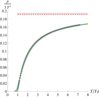
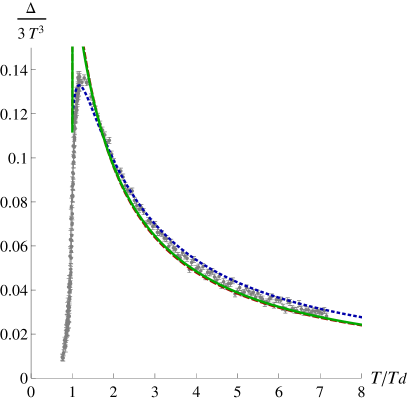
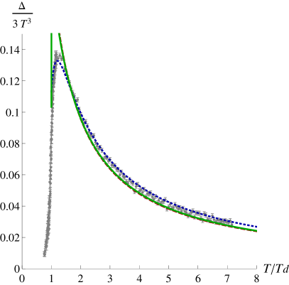
In this section we present the numerical results for the pressure and interaction measure in Figs. 12, 13, 14, 15, and 16 for and compare to the lattice data of Ref. Caselle et al. (2011a). Moreover, we also numerically compute the Polyakov loop, see Figs. 17, 18, and 19. For the renormalized Polyakov loop in dimensions there are no lattice data available so far. All results are obtained within the uniform eigenvalue Ansatz using the one-parameter model, the two-parameter model, and the four-parameter fit. In addition, we present the plots for two different nonperturbative terms, the Vandermonde determinant (48) and the linear term (53).
| Non-pert. | rescale | rescale | ||||
|---|---|---|---|---|---|---|
| SU(2)c Vdm 1 par | 0.000136 | 0.999951 | 0.999998 | 0 | 1 | 1 |
| SU(2)c Vdm 2 par | 0.000054 | 0.99998 | 0.999999 | -0.0141610 | 1 | 1 |
| SU(2)c Vdm 4 par | 0.216395 | 0.921952 | 0.997463 | -0.111553 | 0.937285 | 1.03389 |
| SU(2)c lin 1 par | 0.000010 | 0.999996 | 1. | 0 | 1 | 1 |
| SU(2)c lin 2 par | 0.000007 | 0.999997 | 1. | -0.0124482 | 1 | 1 |
| SU(2)c lin 4 par | 0.958075 | 0.654448 | 0.988659 | -0.0977655 | 0.933455 | 1.02394 |
| SU(3)c Vdm 1 par | 0.0134234 | 0.992711 | 0.999587 | 0 | 1 | 1 |
| SU(3)c Vdm 2 par | 0.0103609 | 0.994374 | 0.999681 | -0.0298485 | 1 | 1 |
| SU(3)c Vdm 4 par | 0.118785 | 0.935495 | 0.996459 | -0.107797 | 0.968308 | 1.03236 |
| SU(3)c lin 1 par | 0.563232 | 0.75861 | 0.991713 | 0 | 1 | 1 |
| SU(3)c lin 2 par | 0.582769 | 0.750236 | 0.991426 | - 0.000000 | 1 | 1 |
| SU(3)c lin 4 par | 0.813344 | 0.651416 | 0.988387 | -0.104560 | 0.967003 | 1.03043 |
| SU(4)c Vdm 1 par | 1.30689 | 0.159154 | 0.967712 | 0 | 1 | 1 |
| SU(4)c Vdm 2 par | 0.155114 | 0.900201 | 0.996168 | -0.0678792 | 1 | 1 |
| SU(4)c Vdm 4 par | 0.118808 | 0.92356 | 0.997172 | -0.159610 | 0.980361 | 1.03790 |
| SU(4)c lin 1 par | 3.40505 | -0.547142 | 0.965097 | 0 | 1 | 1 |
| SU(4)c lin 2 par | 1.26641 | 0.424584 | 0.987019 | -0.0640259 | 1 | 1 |
| SU(4)c lin 4 par | 0.595675 | 0.729345 | 0.994108 | -0.159541 | 0.980182 | 1.03626 |
| SU(5)c Vdm 1 par | 2.28362 | -0.612346 | 0.956678 | 0 | 1 | 1 |
| SU(5)c Vdm 2 par | 0.0504081 | 0.96441 | 0.999044 | -0.0665565 | 1 | 1 |
| SU(5)c Vdm 4 par | 0.103883 | 0.926654 | 0.998076 | -0.114687 | 0.996903 | 1.02406 |
| SU(5)c lin 1 par | 9.3767 | -3.37883 | 0.931681 | 0 | 1 | 1 |
| SU(5)c lin 2 par | 0.693992 | 0.675912 | 0.994944 | -0.0642173 | 1 | 1 |
| SU(5)c lin 4 par | 0.689758 | 0.677889 | 0.995089 | -0.114556 | 0.996670 | 1.02339 |
| SU(6)c Vdm 1 par | 3.26897 | -1.44726 | 0.951671 | 0 | 1 | 1 |
| SU(6)c Vdm 2 par | 0.0536514 | 0.959835 | 0.999207 | -0.0722529 | 1 | 1 |
| SU(6)c Vdm 4 par | 0.0927683 | 0.93055 | 0.998666 | -0.120177 | 1.00121 | 1.02807 |
| SU(6)c lin 1 par | 5.54761 | -1.63022 | 0.97006 | 0 | 1 | 1 |
| SU(6)c lin 2 par | 0.634597 | 0.699126 | 0.996575 | -0.0711707 | 1 | 1 |
| SU(6)c lin 4 par | 0.598767 | 0.716114 | 0.996855 | -0.120282 | 1.00109 | 1.02763 |
The free parameters of the model are adjusted by fitting the lattice pressure of Ref. Caselle et al. (2011a) for for all . Table 2 lists the parameters for all cases studied in this work, where we introduce the following notation: “1 par” for the one-parameter model, “2 par” for the two-parameter model, and “4 par” for the four-parameter fit. Furthermore, “lin” denotes the linear term and “Vdm” the Vandermonde determinant. The parameters and are not free, they are functions of . In “1 par” we use as the single free parameter to fit the lattice data. In “2 par” we add a second free parameter,
| (96) |
to include the effects of the bag constant , see Sec. IV.7. In “4 par” we further allow for small shifts in , and in the perturbative constant (89), in order to encompass other possible nonperturbative effects not included in our matrix model.
Overall, the change in and with the number of colors becomes weaker with increasing number of parameters. Moreover, for the Vandermonde determinant the variation of and with is milder than for the linear nonperturbative term. In the one-parameter model and change significantly with increasing and/or when switching between the linear and the Vandermonde term. For the two-parameter model, we find that as increases, and approach the same values as in the four-parameter fit which gives quantitatively the best fits to the lattice data.
In the four-parameter fit tends to decrease with increasing number of colors. Moreover, the value of in the four-parameter fit is significantly smaller than for the one-parameter model. Typically, drops by an order of magnitude as one goes from one to four parameters. Notably, for the Vandermonde determinant assumes approximately the same value for all in the four-parameter fit, . Finally, we notice that for all scenarios studied in this work, is approximately constant, presumably because it is fixed by the high- behavior.

V.1 Pressure and interaction measure
V.1.1 One- and two-parameter model
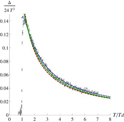
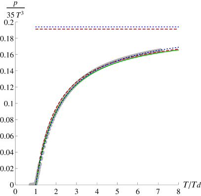
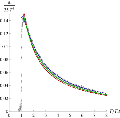
The one- and two-parameter matrix models reproduce the lattice data remarkably well within the considered temperature region . An important result is that with only one free parameter, we can already describe the deviation from an ideal gluon gas observed on the lattice at . Regarding the dependence on the number of colors, we confirm the general trend observed on the lattice: when scaled by the number of gluons, , the pressure and the interaction measure only marginally change with varying . For all , we find that including the effects of the bag constant allows for a better agreement with the lattice data than the one-parameter model.
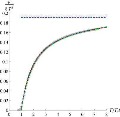
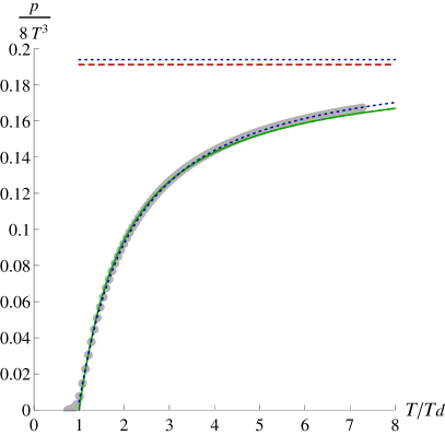
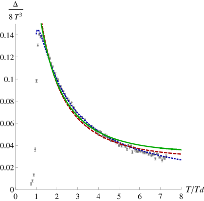
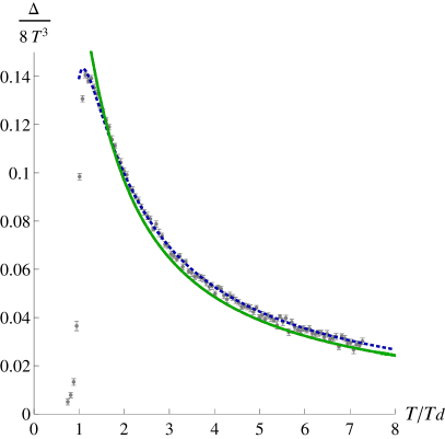
Despite the overall good correspondence, we notice that at high temperatures the deviation between our results and the lattice pressure slightly increases. In addition, we are not able to reproduce the correct shape for the peak of the interaction measure residing near . Therefore, we also present the results using the four-parameter fit.
An interesting observation is that the two-parameter model can be seen as an interpolation between the one-parameter model for and the four-parameter fit for larger values of .

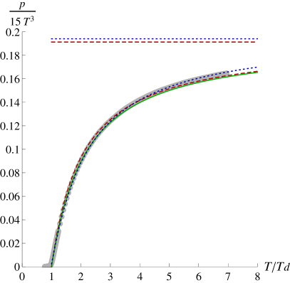
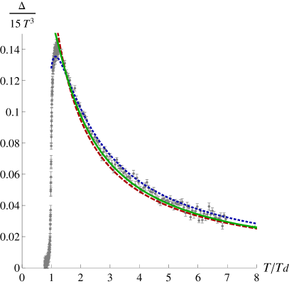
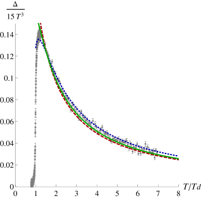
V.1.2 Four-parameter fit
The four-parameter fit quantitatively improves the agreement with lattice data for the pressure and interaction measure. The shift in is introduced to account for possible glueballs effects not included in our model, while the shift in is motivated by possible higher-order loop corrections to the perturbative potential. Furthermore, finite-volume effects present on the lattice close to and at high temperatures may also slightly shift the values of and .

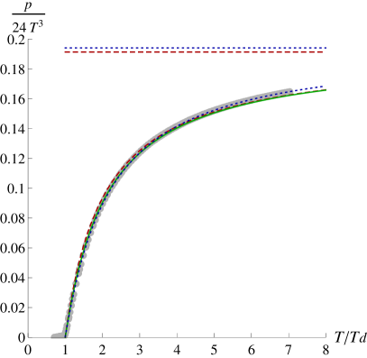

V.1.3
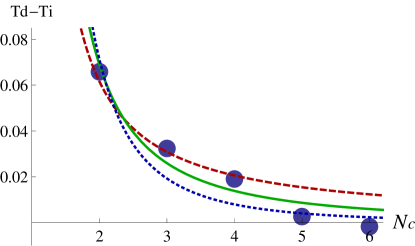
In Fig. 20 we plot the shift in the critical temperature, , as a function of , together with three different fit functions, and . The intercept temperature corresponds to the best estimate for the temperature where the pressure vanishes. Notably, the values for are rather small and rapidly decrease with , approximately as indicating that any possible glueball contribution becomes less important for larger . This is in accordance with general expectations that glueballs become suppressed by a factor above .
V.1.4
Concerning the shift in the perturbative constant it is interesting to note that it remains approximately constant when varying the numbers of colors, , supporting the expectation that including higher-order loop perturbative corrections may account for the small deviation from lattice data in the perturbative limit.


V.2 Polyakov loop
Using the parameters determined by fitting the lattice pressure, we also plot the Polyakov loop.
V.2.1
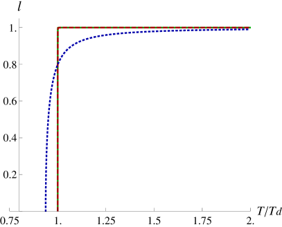
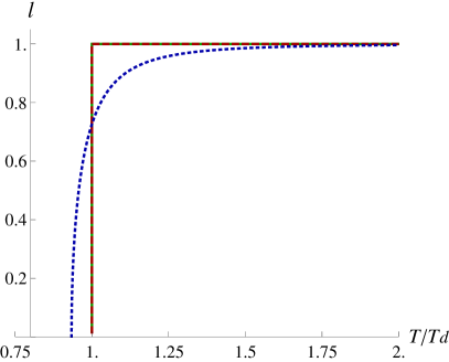
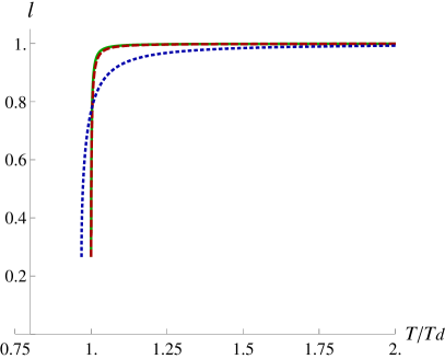
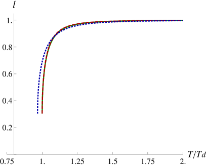
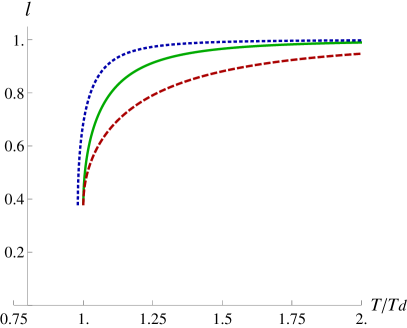
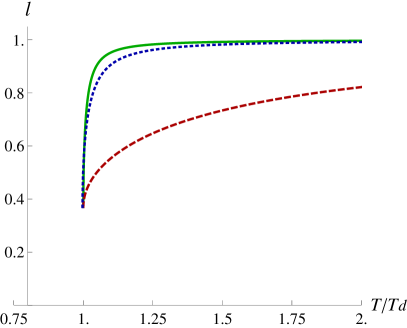
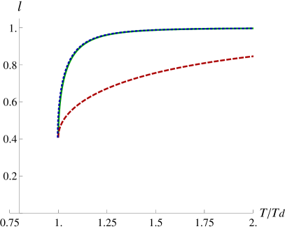
In the one- and two-parameter model, the best fits to the lattice pressure for are obtained in the cases, where the system instantly merges from the confining vacuum, , to the perturbative vacuum, , above . Consequently, for two colors the Polyakov loop rises abruptly from to , see Fig. 17. This is because in our model the Polyakov loop differs from unity only for nonzero values of the condensate , see Eqs. (67) and (68). Strictly speaking, in the presence of a linear or a Vandermonde term the condensate never identically vanishes. Still, the region where is numerically large, is very narrow. As explained in Sec. IV.7, the reason for the shortcoming of the one- and two-parameter model may be that for the glueball contribution to the free energy is not negligible at the phase transition. Therefore, we need to allow for a nonzero pressure at , which is equivalent to shifting the critical temperature, the way it is done in the four-parameter fit.
V.2.2
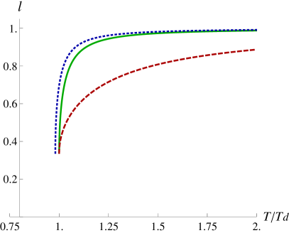
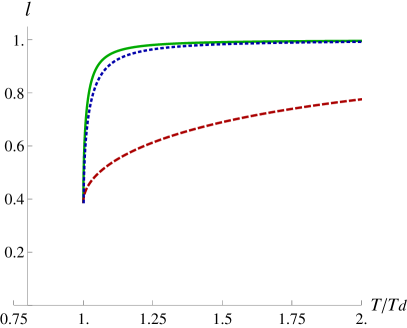
For the phase transition is of first order. Thus, the expectation value of the Polyakov loop jumps from zero to a nonzero value at the critical temperature, and then approaches unity at asymptotically high temperatures.
In the one-parameter model, the region where the Polyakov loop notably differs from unity increases with . In the four-parameter fit, on the other hand, the plots for the Polyakov loop only slightly change when varying , similar to other thermodynamical observables. Interestingly, the two-parameter plots for the Polyakov loop essentially coincide with the one-parameter model for , while for they are very close to the results of the four-parameter fit. Note that for any possible glueball contribution near the phase transition is already sufficiently suppressed by the factor . As a consequence, for all models considered in this work provide plausible plots for the Polyakov loop, while for only the four-parameter fit allows for reasonable results.
V.2.3 Transition region
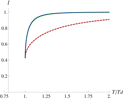
From the Polyakov loop, we can directly determine the transition range where the condensate is nonvanishing. This is the region where the dependent nonperturbative terms enter the thermodynamical quantities. In the one-parameter model, the transition range is practically zero for . It becomes broader with increasing number of colors, and ends up approximately at for . In the four-parameter fit, the transition region is broadly independent of and extends up to . Similar results are obtained in the two-parameter model, except for the case , where the transition range vanishes. Remarkably, this is very close to the results in dimensions, where the Polyakov loop notably differs from unity up to .
VI The potential for a general parametrization of the background field
In the previous sections IV and V we have presented a detailed study of the region between the perturbative and confining vacuum, , where the Polyakov loop varies from zero to unity, using the uniform eigenvalue Ansatz (64). In this section we extend the parametrization of the background field to a complete basis of diagonal generators of the Lie algebra. Thus, the Polyakov loop may take any value within the solid lines of Fig. 1.
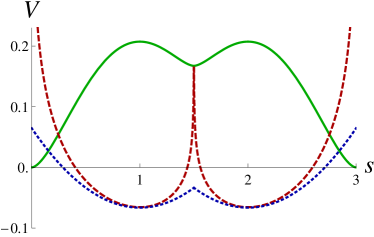
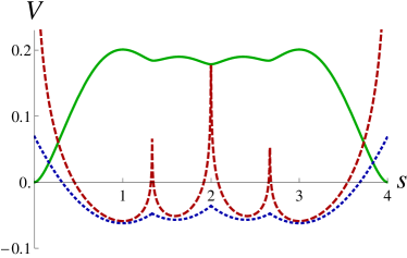
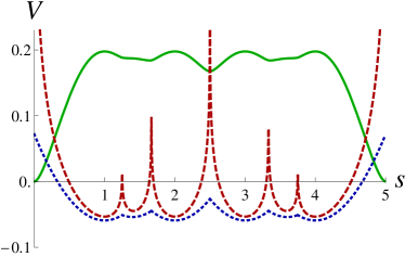
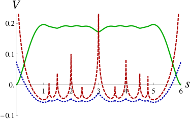
First we look at the potential along the uniform eigenvalue Ansatz beyond the confining vacuum, . Figure 21 shows the perturbative potential (42), the Vandermonde term , and the linear term (53) for up to . In addition, in Fig. 22 we plot the effective potential in the presence of the Vandermonde term for . The functions , , and are all periodic in and symmetric with respect to .
An interesting observation is that the perturbative potential exhibits local minima at . Notably, there appear also extrema in the nonperturbative contributions and in the effective potential. For the Vandermonde term exhibits local minima and divergences which partly coincide with the local minima in the perturbative potential. The same arguments apply to the effective potential. For the linear term the results are qualitatively similar, except that the divergences disappear. However, it is instructive to focus first only on the perturbative potential which, in contrast to the nonperturbative and effective potential, does not depend on the details of the model.
As demonstrated in Fig. 3, in the uniform eigenvalue Ansatz the Polyakov loop takes always values along the real axis within the solid lines of Fig. 1. Therefore, the local minima in the perturbative potential at represent possible physical solutions. It is important to point out, however, that the extremal points present in the potential beyond the confining vacuum do not affect the results of our study between the perturbative and confining vacuum. Nevertheless, an interesting question is if the local minima are metastable solutions, or just saddle-points. For this purpose, we have to check if they are stable in the direction transverse to the uniform eigenvalue Ansatz (64), i.e., if they correspond to local minima in the entire -dimensional space spanned by the orthogonal diagonal generators of .
This can be done by looking for local minima in the perturbative potential in the presence of a background field,
| (97) |
where is a diagonal matrix parametrized as
| (98) |
The matrices and form a set of orthogonal diagonal generators of the Lie algebra, while and are the associated parameters. As elements of the Lie algebra, the diagonal generators must be traceless and real. In order to obtain an orthogonal basis, we also require that the inner product between two generators must vanish. Moreover, it is convenient to normalize the generators in such a way that the perturbative potential exhibits the same periodicity, , and symmetry,
| (99) |
along all as along . Therefore, it is sufficient to restrict the search for local minima to the range
VI.1
First we consider . The perturbative potential has a local minimum in the direction,
| (100) |
at , where . For the generator orthogonal to it is convenient to choose
| (101) |
In order to check if the local minimum at is stable in the direction transverse to , we compute the perturbative potential in the plane spanned by and
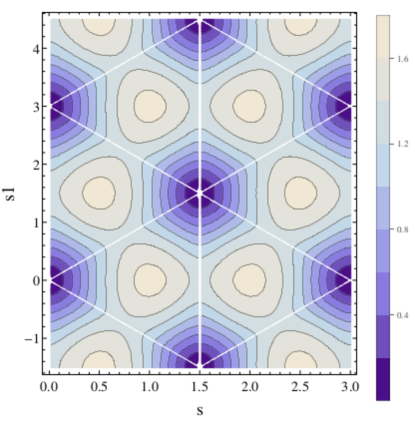
Figure 23 shows a density plot for , where is a diagonal matrix for the background field (97) parametrized as
| (102) |
For , there is one global minimum at corresponding to the perturbative vacuum, where . But there is no local minimum at and . Taking the periodicity of the perturbative potential into account, the other global minima in Fig. 23 are all degenerate with the perturbative vacuum at .
VI.2
VI.2.1 Minima along the uniform eigenvalue Ansatz
For we find two local minima in the region along the uniform eigenvalue Ansatz,
| (103) |
at and . A symmetric diagonal basis for is obtained by choosing
| (104) |
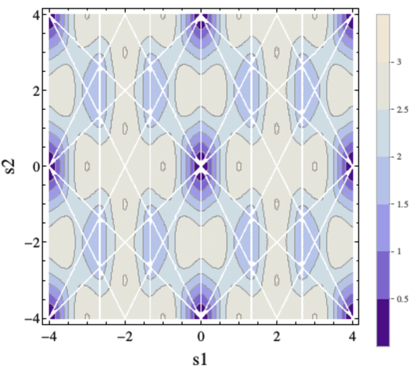
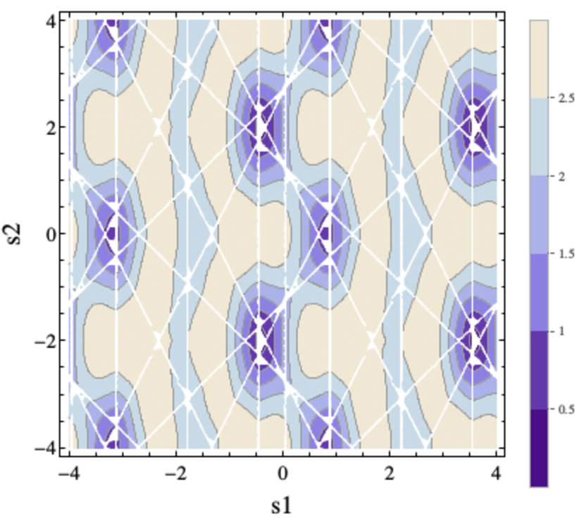
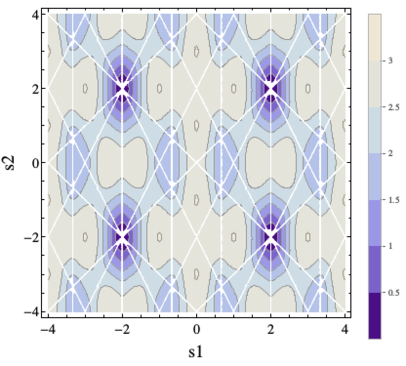
for the remaining two generators orthogonal to . In order to see if the local minima along are metastable or saddle points, we parametrize the matrix as
| (105) |
and plot the perturbative potential in the -plane perpendicular to , at (Fig. 24(a)), (Fig. 24(b)), and (Fig. 24(c)). Considering the periodicity of the perturbative potential, our analysis indicates that, except for degenerate global minima which correspond to the perturbative vacuum at , there are only saddle points along the uniform eigenvalue Ansatz.
VI.2.2 Minima in the entire 3-dimensional volume
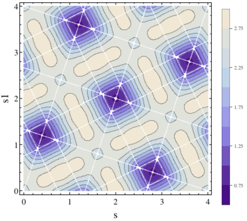
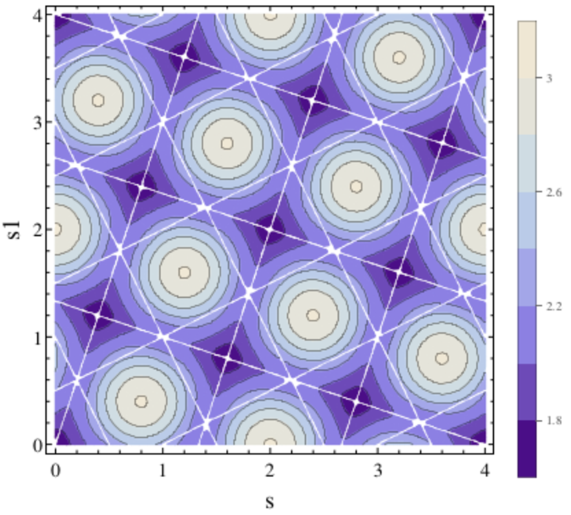
Note that in order to take into account all possible metastable solutions in the perturbative potential, we should ideally look for local minima in the entire -dimensional space. This can be done by plotting slices of the perturbative potential in the -plane along the perpendicular direction for fixed values of , see Figs. 25 and 26.
We start with Fig. 25(a) which shows a density plot of the perturbative potential in the -plane, spanned by the generators and for . The global and local minima reside at intersections of the white lines which connect the regions where the perturbative potential is minimized. From the intersections we can therefore determine the exact positions of the minima.
Within the considered region there are eight degenerate global minima at , , , , , , , and . Each global minimum exhibits an octagonal structure and is located in the center between eight neighboring maxima which are all degenerate with the confining vacuum at .
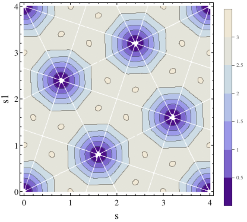
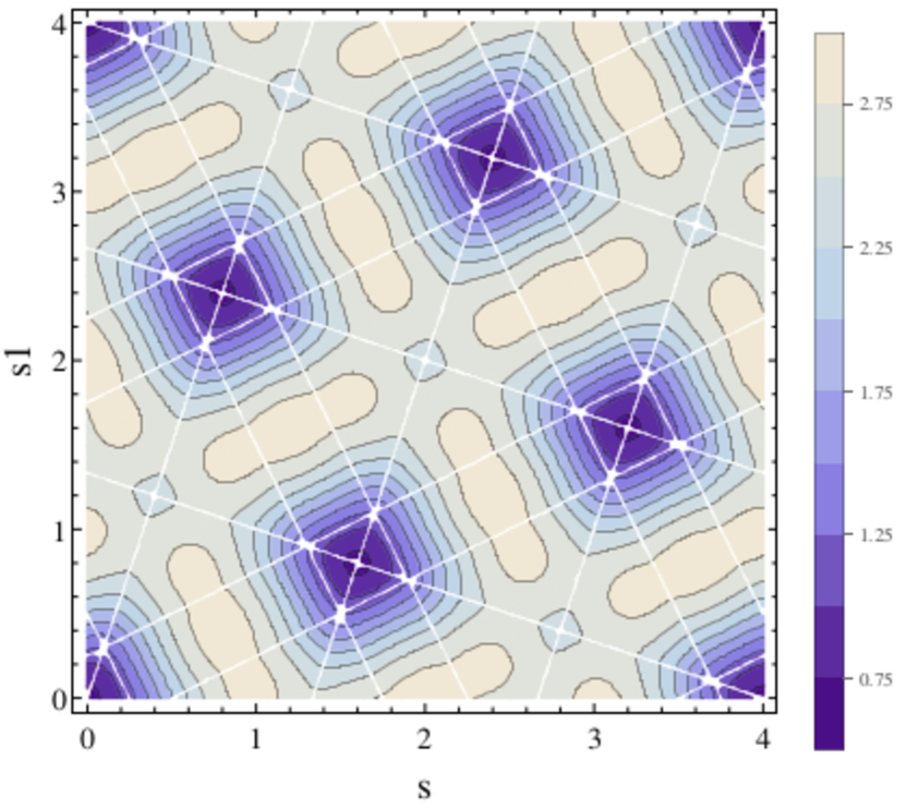

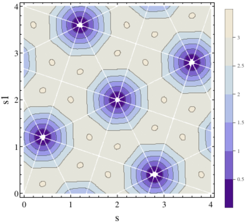


We also find five local minima at , , , , and . Their coordinates are offset from the global minima by the vector . Each local minimum resides in the center between four neighboring global minima.
As we start moving along the direction, the global and local minima begin to transform into one another: the global minima become shallower, while the local minima get deeper, see Fig. 25(b). Consequently, at all minima become degenerate, see Fig. 25(c). Moving further to , Fig. 26(a), the roles of the minima interchange: the former global minima are transformed into local minima and vice versa. Finally, at , we recover the same pattern as in the initial state at see Fig. 25(a).
Overall, we find that the structure of the perturbative potential in the entire three-dimensional space spanned by the diagonal generators , , and resembles a crystal, and that the edges of the elementary cell are spanned by the three vectors and The periodicity of these elementary cells is given by the norm of the vectors,
Summarizing our study for and demonstrates that there are only global minima in the perturbative potential which are all degenerate with the perturbative vacuum of our uniform eigenvalue Ansatz at , where . Moreover, all maxima in the perturbative potential are degenerate with the confining vacuum at and , where . But we find no indication of metastable solutions.
Thus, we verify that the perturbative potential exhibits no other stationary points except for the ones at and along the uniform eigenvalue Ansatz studied in this work. Consequently, we confirm that employing any other parametrization of the background field, which takes us from the perturbative vacuum (minimum) to the confining vacuum (neighboring maximum), will not change the physics.
An interesting outlook for future projects would be to extend the present analysis to . We can also look for stationary points by solving the stationary conditions
| (106) |
Furthermore, it would be certainly useful to look for local minima in the full effective potential. In the present work, however, we do not further address the question of possible metastable solutions.
VII Conclusions
We have used an effective matrix model to study the deconfinement phase transition in pure gauge theories in dimensions. The effective potential was constructed as a sum of a perturbative and a nonperturbative part. The perturbative potential was computed to one-loop order in the presence of a constant background field. In order to model the transition to confinement, we then constructed appropriate -dependent and -independent nonperturbative terms, motivated by lattice results for the pressure and interaction measure.
The analytical calculations were performed for general and in the large- limit. We also presented the numerical solution for the potential using the uniform eigenvalue ansatz which guaranties that the Polyakov loop is real. The free parameters of the model were adjusted by fitting to the lattice pressure of Ref. Caselle et al. (2011a). We have shown the pressure and interaction measure for and compared to the lattice data of Ref. Caselle et al. (2011a). Overall, the results exhibit a mild sensitivity with respect to the details of the -dependent nonperturbative terms.
Using one and two free parameters, we already obtain a good agreement with the lattice data. Notably, with only one free parameter we reproduce the correct temperature dependence for the deviation from an ideal gluon gas at . As observed on the lattice, we also find a small dependence on the number of colors for the pressure and the interaction measure, except for the factor .
In order to further improve the agreement with lattice close to the deconfinement temperature and at high , we introduced a four-parameter fit. This fit is constructed from the two-parameter model by allowing for a shift in , and in the perturbative limit of the pressure, . The shift in is rather small and rapidly vanishes with increasing number of colors. This supports the general expectation that any possible glueball contribution becomes suppressed by a factor at the phase transition. The shift in is approximately constant for all , .
The four-parameter fit allows for a very good agreement with the lattice results at all temperatures. We stress however, that the four-parameter fit is just an approximation to a more complete theory properly incorporating the physics in the confined phase. The general trend we observe is that the two-parameter model can be regarded as an interpolation between the one-parameter model for , and the four-parameter fit for larger .
Using the parameters determined by fitting the lattice pressure, we have also plotted the Polyakov loop. We find that the transition region, where the system exhibits a nonvanishing condensate for is broadly independent of the number of colors and extends up to . This is very close to the results obtained in Dumitru et al. (2012). So far, the renormalized Polyakov loop has not yet been computed on the lattice in dimensions. The corresponding lattice data could help to clarify the role of nonperturbative effects in the deconfined phase.
It would be certainly useful, to extend the matrix model to a more general effective theory including the physics in the confined phase. Another interesting project would be to study the interface tension which gives the tunneling probability between different vacua of the system. Finally, we could include dynamical quarks, as was done in in Ref. Kashiwa et al. .
Acknowledgements.
The authors would like to thank Marco Panero for kindly sharing the lattice data of Ref. Caselle et al. (2011a). We also thank Dirk H. Rischke, Nuno Cardoso and Marco Panero for valuable discussions. The research of R.D.P. is supported by the U.S. Department of Energy under contract #DE-AC02-98CH10886. E. S. thanks the hospitality of RIKEN/BNL and CFTP. The research of P.B. is supported by the CFTP grant PEST-OE/FIS/UI0777/2011, the FCT grant CERN/FP/123612/2011, and the CRUP/DAAD exchange A10/10.References
- Caselle et al. (2011a) M. Caselle, L. Castagnini, A. Feo, F. Gliozzi, U. Gursoy, et al., (2011a), arXiv:1111.0580 [hep-th] .
- Gopakumar and Gross (1995) R. Gopakumar and D. J. Gross, Nucl.Phys. B451, 379 (1995), arXiv:hep-th/9411021 [hep-th] .
- Dumitru et al. (2011) A. Dumitru, Y. Guo, Y. Hidaka, C. P. Korthals Altes, and R. D. Pisarski, Phys.Rev. D83, 034022 (2011), arXiv:1011.3820 [hep-ph] .
- Dumitru et al. (2012) A. Dumitru, Y. Guo, Y. Hidaka, C. P. K. Altes, and R. D. Pisarski, Phys.Rev. D86, 105017 (2012), arXiv:1205.0137 [hep-ph] .
- Bicudo et al. (2013) P. Bicudo, R. D. Pisarski, and E. Seel, (2013), arXiv:1306.2943 [hep-ph] .
- Karsch (2002) F. Karsch, Lect.Notes Phys. 583, 209 (2002), arXiv:hep-lat/0106019 [hep-lat] .
- Teper (1999) M. J. Teper, Phys.Rev. D59, 014512 (1999), arXiv:hep-lat/9804008 [hep-lat] .
- Johnson and Teper (2002) R. W. Johnson and M. J. Teper, Phys.Rev. D66, 036006 (2002), arXiv:hep-ph/0012287 [hep-ph] .
- Meyer and Teper (2003) H. B. Meyer and M. J. Teper, Nucl.Phys. B668, 111 (2003), arXiv:hep-lat/0306019 [hep-lat] .
- Lucini and Teper (2002) B. Lucini and M. Teper, Phys.Rev. D66, 097502 (2002), arXiv:hep-lat/0206027 [hep-lat] .
- Bursa and Teper (2006) F. Bursa and M. Teper, Phys.Rev. D74, 125010 (2006), arXiv:hep-th/0511081 [hep-th] .
- Bialas et al. (2009) P. Bialas, L. Daniel, A. Morel, and B. Petersson, Nucl.Phys. B807, 547 (2009), arXiv:0807.0855 [hep-lat] .
- Liddle and Teper (2008) J. Liddle and M. Teper, (2008), arXiv:0803.2128 [hep-lat] .
- Caselle et al. (2011b) M. Caselle, L. Castagnini, A. Feo, F. Gliozzi, and M. Panero, JHEP 1106, 142 (2011b), arXiv:1105.0359 [hep-lat] .
- Bialas et al. (2012) P. Bialas, L. Daniel, A. Morel, and B. Petersson, (2012), arXiv:1211.3304 [hep-lat] .
- Moshe and Zinn-Justin (2003) M. Moshe and J. Zinn-Justin, Phys.Rept. 385, 69 (2003), arXiv:hep-th/0306133 [hep-th] .
- Boyd et al. (1996) G. Boyd, J. Engels, F. Karsch, E. Laermann, C. Legeland, et al., Nucl.Phys. B469, 419 (1996), arXiv:hep-lat/9602007 [hep-lat] .
- Lucini and Teper (2001) B. Lucini and M. Teper, JHEP 0106, 050 (2001), arXiv:hep-lat/0103027 [hep-lat] .
- Teper (2002) M. Teper, , 108 (2002), arXiv:hep-ph/0203203 [hep-ph] .
- Umeda et al. (2009) T. Umeda, S. Ejiri, S. Aoki, T. Hatsuda, K. Kanaya, et al., Phys.Rev. D79, 051501 (2009), arXiv:0809.2842 [hep-lat] .
- Borsanyi et al. (2011) S. Borsanyi, G. Endrodi, Z. Fodor, S. Katz, and K. Szabo, (2011), arXiv:1104.0013 [hep-ph] .
- Borsanyi et al. (2012) S. Borsanyi, G. Endrodi, Z. Fodor, S. D. Katz, S. Krieg, et al., (2012), arXiv:1204.0995 [hep-lat] .
- Lucini and Panero (2012) B. Lucini and M. Panero, (2012), arXiv:1210.4997 [hep-th] .
- Pisarski (2000) R. D. Pisarski, Phys.Rev. D62, 111501 (2000), arXiv:hep-ph/0006205 [hep-ph] .
- Meisinger et al. (2002) P. N. Meisinger, T. R. Miller, and M. C. Ogilvie, Phys.Rev. D65, 034009 (2002), arXiv:hep-ph/0108009 [hep-ph] .
- Meisinger and Ogilvie (2002) P. N. Meisinger and M. C. Ogilvie, Phys.Rev. D65, 056013 (2002), arXiv:hep-ph/0108026 [hep-ph] .
- Dumitru et al. (2004) A. Dumitru, Y. Hatta, J. Lenaghan, K. Orginos, and R. D. Pisarski, Phys.Rev. D70, 034511 (2004), arXiv:hep-th/0311223 [hep-th] .
- Oswald and Pisarski (2006) M. Oswald and R. D. Pisarski, Phys.Rev. D74, 045029 (2006), arXiv:hep-ph/0512245 [hep-ph] .
- Pisarski (2006) R. D. Pisarski, Phys.Rev. D74, 121703 (2006), arXiv:hep-ph/0608242 [hep-ph] .
- Pisarski (2007) R. D. Pisarski, Prog.Theor.Phys.Suppl. 168, 276 (2007), arXiv:hep-ph/0612191 [hep-ph] .
- Hidaka and Pisarski (2008) Y. Hidaka and R. D. Pisarski, Phys.Rev. D78, 071501 (2008), arXiv:0803.0453 [hep-ph] .
- Hidaka and Pisarski (2009a) Y. Hidaka and R. D. Pisarski, Phys.Rev. D80, 036004 (2009a), arXiv:0906.1751 [hep-ph] .
- Hidaka and Pisarski (2009b) Y. Hidaka and R. D. Pisarski, Phys.Rev. D80, 074504 (2009b), arXiv:0907.4609 [hep-ph] .
- Hidaka and Pisarski (2010) Y. Hidaka and R. D. Pisarski, Phys.Rev. D81, 076002 (2010), arXiv:0912.0940 [hep-ph] .
- Pisarski and Skokov (2012) R. D. Pisarski and V. V. Skokov, Phys.Rev. D86, 081701 (2012), arXiv:1206.1329 [hep-th] .
- (36) K. Kashiwa, R. D. Pisarski, and V. V. Skokov, Phys.Rev. D85, 114029, arXiv:1205.0545 [hep-ph] .
- Sasaki and Redlich (2012) C. Sasaki and K. Redlich, (2012), arXiv:1204.4330 [hep-ph] .
- Ruggieri et al. (2012) M. Ruggieri, P. Alba, P. Castorina, S. Plumari, C. Ratti, et al., (2012), arXiv:1204.5995 [hep-ph] .
- Diakonov et al. (2012) D. Diakonov, C. Gattringer, and H.-P. Schadler, (2012), arXiv:1205.4768 [hep-lat] .
- Ogilvie (2012) M. C. Ogilvie, J.Phys. A45, 483001 (2012), arXiv:1211.2843 [hep-th] .
- Kashiwa and Pisarski (2013) K. Kashiwa and R. D. Pisarski, (2013), arXiv:1301.5344 [hep-ph] .
- Lin et al. (2013) S. Lin, R. D. Pisarski, and V. V. Skokov, (2013), arXiv:1301.7432 [hep-ph] .
- Bialas et al. (2000) P. Bialas, A. Morel, B. Petersson, K. Petrov, and T. Reisz, Nucl.Phys. B581, 477 (2000), arXiv:hep-lat/0003004 [hep-lat] .
- Bialas et al. (2005) P. Bialas, A. Morel, and B. Petersson, Nucl.Phys. B704, 208 (2005), arXiv:hep-lat/0403027 [hep-lat] .
- Bialas et al. (2010) P. Bialas, L. Daniel, A. Morel, and B. Petersson, Nucl.Phys. B836, 91 (2010), arXiv:0912.0206 [hep-lat] .
- Bhattacharya et al. (1992) T. Bhattacharya, A. Gocksch, C. P. Korthals Altes, and R. D. Pisarski, Nucl.Phys. B383, 497 (1992), arXiv:hep-ph/9205231 [hep-ph] .
- Bhattacharya et al. (1991) T. Bhattacharya, A. Gocksch, C. P. Korthals Altes, and R. D. Pisarski, Phys.Rev.Lett. 66, 998 (1991).
- Korthals Altes et al. (1997) C. Korthals Altes, A. Michels, M. A. Stephanov, and M. Teper, Phys.Rev. D55, 1047 (1997), arXiv:hep-lat/9606021 [hep-lat] .
- Gross et al. (1981) D. J. Gross, R. D. Pisarski, and L. G. Yaffe, Rev.Mod.Phys. 53, 43 (1981).
- D’Hoker (1981) E. D’Hoker, Nucl.Phys. B180, 341 (1981).
- D’Hoker (1982a) E. D’Hoker, Nucl.Phys. B200, 517 (1982a).
- D’Hoker (1982b) E. D’Hoker, Nucl.Phys. B201, 401 (1982b).
- Kajantie et al. (1997) K. Kajantie, M. Laine, K. Rummukainen, and M. E. Shaposhnikov, Nucl.Phys. B503, 357 (1997), arXiv:hep-ph/9704416 [hep-ph] .
- Rischke (2004) D. H. Rischke, Prog.Part.Nucl.Phys. 52, 197 (2004), arXiv:nucl-th/0305030 [nucl-th] .
- Belyaev and Eletsky (1990) V. Belyaev and V. Eletsky, Z.Phys. C45, 355 (1990).
- Enqvist and Kajantie (1990) K. Enqvist and K. Kajantie, Z.Phys. C47, 291 (1990).
- Unsal and Yaffe (2008) M. Unsal and L. G. Yaffe, Phys.Rev. D78, 065035 (2008), arXiv:0803.0344 [hep-th] .
- von Smekal et al. (2011) L. von Smekal, S. R. Edwards, and N. Strodthoff, AIP Conf.Proc. 1343, 212 (2011), arXiv:1012.1712 [hep-ph] .
- Strodthoff et al. (2010) N. Strodthoff, S. R. Edwards, and L. von Smekal, PoS LATTICE2010, 288 (2010), arXiv:1012.0723 [hep-lat] .
- Hagedorn (1965) R. Hagedorn, Nuovo Cim.Suppl. 3, 147 (1965).
- Cohen and Krejcirik (2011) T. D. Cohen and V. Krejcirik, JHEP 1108, 138 (2011), arXiv:1104.4783 [hep-th] .