Shannon-Rényi entropies and participation spectra across 3d criticality
Abstract
Universal features in the scalings of Shannon-Rényi entropies of many-body groundstates are studied for interacting spin- systems across (2+1) dimensional critical points, using quantum Monte Carlo simulations on dimerized and plaquettized Heisenberg models on the square lattice. Considering both full systems and line shaped subsystems, symmetry breaking on the Néel ordered side of the transition is characterized by the presence of a logarithmic term in the scaling of Shannon-Rényi entropies, which is absent in the disordered gapped phase. Such a difference in the scalings allows to capture the quantum critical point using Shannon-Rényi entropies for line shaped subsystems of length embedded in tori, as the smaller subsystem entropies are numerically accessible to much higher precision than for the full system. Most interestingly, at the quantum phase transition an additive subleading constant emerges in the critical scaling of the line Shannon-Rényi entropy . This number appears to be universal for 3d criticality, as confirmed for the finite-temperature transition in the 3d antiferromagnetic spin- Heisenberg model. Additionally, the phases and phase transition can be detected in several features of the participation spectrum, consisting of the diagonal elements of the reduced density matrix of the line subsystem. In particular the Néel ordering transition can be simply understood in the basis by a confinement mechanism of ferromagnetic domain walls.
I Introduction
How do coefficients of a wave-function change at continuous quantum phase transitions? In a given basis, this question can be addressed by monitoring the behavior of (inverse) participation ratios, which have a long history e.g. in localization physics Wegner (1980); Fyodorov and Mirlin (1992); Evers and Mirlin (2000, 2008). More recently, the study of related quantities such as Shannon-Rényi entropies (which quantify the localization of the wave-function in a given basis) in many-body problems has revealed an intriguing aspect: subleading terms in the finite-size scaling of these quantities appear to carry universal information, characteristic of the physics contained in the ground-state wave-functionStéphan et al. (2009, 2010, 2011); Zaletel et al. (2011); Luitz et al. (2014). For instance, they can characterize the presence of broken continuous or discrete symmetry breaking in the ground-state, as well as information on the universality class of continuous phase transitions. Most previous studiesStéphan et al. (2009, 2010); Zaletel et al. (2011); Stéphan et al. (2011); Atas and Bogomolny (2012); Um et al. (2012); Alcaraz and Rajabpour (2013) on this topic focused on one-dimensional quantum systems, where both analytical and numerical studies are easiest. In particular, dealing with the exponentially growing size of the Hilbert space of many-body problems, while maintaining a large enough total system size to study finite-size dependence, is a hurdle to surmount.
Recently, we have introduced in Ref. Luitz et al., 2014 convenient numerical methods to study the Shannon-Rényi entropies of many-body systems through a quantum Monte Carlo (QMC) sampling of the ground-state wave function. This method allows studies of much larger systems than previously accessible in numerical calculations, which is necessary for the analysis of universal behavior at continuous quantum phase transitions where physical correlation lengths diverge.
Here, we will study this problem for a non-trivial, yet well-understood quantum phase transition in two-dimensional quantum magnetism: the transition between a Néel antiferromagnet and a quantum paramagnet in two quantum spin Heisenberg models with varying antiferromagnetic couplings, namely two-dimensional coupled dimers and plaquettes (see Fig. 1). The variation of the ratio of two exchange couplings allows to couple isolated paramagnetic units (at ) to form a two-dimensional antiferromagnet (at ) which spontaneously breaks symmetry at zero temperature. A quantum critical point at in the 3d universality classTroyer et al. (1997); Matsumoto et al. (2001); Wang et al. (2006); Albuquerque et al. (2008); Wenzel and Janke (2009); Sandvik (2010) separates the quantum disordered and Néel ordered phases.
The first part of the paper (Sec. III) is devoted to the study of the behavior of subleading terms in the SR entropies of the ground-state of Heisenberg magnets. Given a density matrix , the SR entropies are defined as:
| (1) |
where are states of the computational basis in which SR entropies are calculated. Note that the choice of the natural logarithm (base ) fixes the units of SR entropies to “nats”.
We will first consider in Sec. III.1 the SR entropy of the full system composed of interacting spins on a square lattice, that is choosing in Eq. (1) to be the full density matrix of the ground state . SR entropies are generally found to have a leading behavior which is extensiveAtas and Bogomolny (2012); Luitz et al. (2014) where the pre-factor (for spin systems) depends on details of the model ( in that case). In the basis considered throughout this work, we naturally expect to be ‘small’ in the Néel phase, and ‘large’ in the quantum disordered phase. This is easily understood by considering the limit , where . Here, is the (modulus squared of the) maximal coefficient of the groundstate wave-function expanded in the basis. For antiferromagnetic systems, this is the coefficient of the Néel state , which is expected to be much larger in the antiferromagnetically ordered phase than in the disordered phase. In the antiferromagnetic phase, the groundstate spontaneously breaks the continuous symmetry and our previous work Luitz et al. (2014) showed that this is reflected in a subleading logarithmic correction: . In the disordered phase, no symmetry is broken and the subleading term is in general a universal constant (expected to be zero in the paramagnetic phase discussed in this paper).
For this first part of the paper (Sec. III), we will consider the case essentially for practical purposes. Indeed, is simpler to obtain numerically (within our QMC simulations) and more importantly, the leading term prefactor is smaller ( for all finite ) which ensures that we can reach larger system sizes. Despite these facts, simulations of the SR entropy of full two dimensional systems are limited to relatively small sizes (up to ) close to the quantum phase transition, as the prefactor is still quite large in this region (see also the discussion in appendix A).
To circumvent this, we next consider in Sec. III.2 the scaling of the SR entropy of a subsystem, composed of a single line of size (the geometry of the subsystem is defined in Fig. 1) embedded in a periodic torus. Subsystem SR entropies are defined in analogy to Eq. (1), except that we now consider the reduced density matrix of a subsystem which is obtained by performing a partial trace over the rest of the system :
| (2) |
with , i.e. where the basis state is a tensor product state of subsystems basis states and .
The rationale for choosing a line shaped subsystem is two-fold: first, we physically expect that the SR entropy of the line also contains the information about antiferromagnetic ordering (since for instance the correlation function along the line is defined in terms of diagonal elements of the reduced density matrix). Second, the SR entropy of the line has a leading term , and therefore takes much smaller values than for the full-system SR entropy for the same value of ( scaling versus scaling). This leads to a better accuracy and allows to reach much larger linear sizes in our QMC simulations.
Our results indicate that the SR entropy of the line also shows a sub-leading term in the Néel phase, and a constant term in the disordered phase which turns out to vanish (see below). Quite interestingly, the subleading term right at the quantum phase transition is a constant , which appears to be identical (within error bars) for the two models studied. This suggest that this constant is characteristic of the 3d universality class to which both quantum phase transitions belong. Further simulations of the finite-temperature ordering phase transition of the simple cubic Heisenberg model (also in the same universality class) support this conjecture for antiferromagnetic interactions. We also expect a universal value for the full system, even though the limited accuracy (due to the large value of ) of our simulations does not allow to prove this.
For the verification of the universality of , we have first performed extensive calculations of the spin stiffness in order to extract the best estimate for the value of the transition temperature, , in agreement with Ref. Yasuda et al., 2005.
The SR entropies are global averages of all coefficients of the wave-function and their scaling with the (sub-) system size thus capture correctly phases and phase transitions. It is interesting to ask whether each individual coefficient (or reduced density matrix diagonal element in the case of subsystems) also “sees” the quantum phase transition when is varied – this independently of their scaling with system size, as exemplified with the maximal diagonal entry of the (reduced) density matrix, governing (). Motivated by this question, we study in the second part of the paper (Sec. IV) the behavior of each diagonal element of the reduced density matrix for a line subsystem across the transition. In analogy with the entanglement spectrum Li and Haldane (2008); Calabrese and Lefevre (2008), we define the “participation spectrum” as the set of pseudo-energies . The participation spectrum develops into well-defined bands, which can be classified according to the magnetization and the number of ferromagnetic domain-walls separating segments having different Néel line configurations ( or . Identifying the lowest-lying states in this spectrum allows to understand the quantum phase transition in terms of an effective repulsion between such domain-walls. Even though the participation spectra appear to differ at first glance in the quantum disordered phases of the two studied models, we find that this can be understood easily by classifying states according to the number of strong or weak domain walls (this notion is dictated by the local physics of one of the two models considered). A striking outcome of this analysis is that all individual levels (even corresponding to assumedly irrelevant states such as the fully polarized state) harbor signs of the quantum phase transition, as exemplified for instance by an inflection point (with respect to ) for almost all . We analyze this in detail for the most probable state. Another interesting sign of the quantum phase transition is revealed by the study of the finite-size behavior of the width of the lowest-lying bands. We will finally conclude in Sec. V on the implications of our results while the appendices contain specific details of the QMC procedure used (Appendix A), as well as exact results in the limit of for reference (Appendix B).
Let us begin our paper (Sec. II) by providing useful details on the models studied as well as on the finite-size scaling analysis.
II Models and methods of analysis
The two models (dimerized and plaquettized Heisenberg models) that we study are defined with the same Hamiltonian form:
| (3) |
with and where the two terms correspond to the summation over stronger bonds for columnar dimers (plaquettes) and to the summation over the weaker links between these entities (see Fig. 1). We only consider here, with yielding the homogeneous Heisenberg antiferromagnet on the square lattice. The two models have slightly different critical points at Sandvik (2010) for the columnar dimerized system and Wenzel and Janke (2009) for the plaquettized system. For both models display a disordered ground state separated from excited states by a finite energy gap, whereas for antiferromagnetic Néel long-range order occurs, with a spontaneous breaking of the symmetry. We considered these two models as they are well-established to harbor the same physical content (in particular the quantum phase transitions at belong to the same 3d universality class), yet with different microscopics: this will allow us to discuss universality of the scaling of SR entropies.
We study properties of the groundstates expanded in the basis and note that all results will be identical in any basis obtained by a global transformation, by symmetry of the Hamiltonian. We use the index (respectively ) to denote quantities for the plaquettized (resp. dimerized) model. Considering the results of Ref. Luitz et al., 2014, we will perform fits of the SR entropy of the full system to the following forms:
| (4) |
and
| (5) |
Equivalent forms for the line SR entropy are:
| (6) |
and
| (7) |
Note that in general, one also expects Luitz et al. (2014) further size corrections and .
The second functional forms Eqs. (5) and (7) are of course included into the first forms Eqs. (4) and (6), when the fitting parameters or are found to be zero. However, given the finite values of and that we can reach and the error bars inherent to QMC, the fits to Eqs. (5) and (7) are better controlled (and errors on estimated parameters smaller) by forcing to be zero for systems where no log term is present. Indeed, putting a log term when not needed can result in an acceptable fit where an artificial compensates wrongly underestimated or . For systems where no log term is present, we must have and (respectively and ) for large enough sizes, but this scaling regime might be reached earlier by using the second forms Eqs. (5), (7). Let us finally mention the simple argument that if one is looking for universal constants, then only and can be universal (but not ) in the first forms Eqs. (4) and(6): this is seen by a redefinition of sample size or . With the same reasoning, only can be universal for the second forms Eqs. (5) and (7).
For all fits, we used a rigorous bootstrap analysis in order to provide reliable error bars for fit parameters. Note, however, that these error bars do not contain systematic effects due to finite system sizes. These effects can nevertheless be estimated by comparison of fits over different system size or ranges (“fit windows”, see Ref. Luitz et al., 2014 for details). We also monitored the fit quality (see Ref. Young, 2012) to ascertain the precision of our fits.
III Shannon-Rényi entropies
Throughout this section, we restrict our discussion and analysis to the computationally most accessible SR entropy, when for both the full system () in Sec. III.1 and the line subsystem () in Sec. III.2.
III.1 SR entropy of the full system
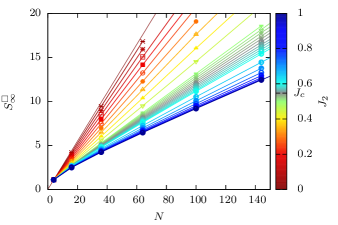
Figure 2 shows our QMC result for of the plaquettized model in the range of accessible entropies (our simulations are limited roughly to as discussed in appendix A), for different values of the parameter in the range .
In the limit of isolated plaquettes, can be exactly (cf. appendix B) shown to be , i.e. a pure linear scaling with no logarithmic or constant terms. In the uniform Heisenberg limit on the other hand, previous results Luitz et al. (2014) have shown the existence of a logarithmic scaling correction with the form Eq. (4) with .
By inspection of the bare SR entropy scaling in Fig. 2, a nonzero logarithmic scaling term can be presumed for the whole ordered phase (with curves clearly bending downwards for smaller system sizes), while for the disordered phase, the scaling appears linear. In order to quantify this, we have performed fits of the Monte Carlo data corresponding to the form Eq. (4). We emphasize that the quality of the fits (in particular the extraction of the logarithmic term) is reduced when only few system sizes are available, which is specially the case in the disordered regime of the phase diagram (due to faster growing with system size). As the situation is worse for the dimerized model (we have for instance , cf. appendix B), we concentrated our analysis for this section on the plaquettized model.
Fig. 3 displays the result of our fits for the prefactor of the logarithmic scaling correction of . The trend with increasing system sizes included in the fit is evident in the ordered phase, as is found to be almost constant with there. In the disordered phase, large finite size effects are observed which are very similar to the oscillations found for the constant term close to the quantum phase transitions of transverse field Ising models Stéphan et al. (2009); Luitz et al. (2014). We expect to vanish in the complete quantum disordered phase (as it is shown analytically for in appendix B) and our data are consistent with this expectation, although the numerical precision is not sufficient for a definite answer. The lack of availability of larger also prevents us to conclude if there is a universal number (and what is its numerical value) in the Néel phase, even though the plateau shape of the curves tend to indicate that this is possible. The actual universal value (if any) may be quite larger than the maximum value here (found to be for the fit window with the largest ), as can be seen by the shift of the curves when smaller sizes are removed from the fit.
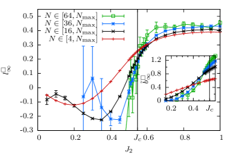
The inset of Fig. 3 shows our fit results for the same fit windows as in the main panel for as obtained from fits to Eq. (5) close to . In this region, large finite size effects are hampering a reliable extraction of the constant but a lower bound for the value at the critical point can be perceived. Results from fit windows excluding smaller system sizes seem to indicate that vanishes in the disordered phase.
It would be of clear interest to increase the maximum size in the simulation to have a larger fitting range, but this is not possible with the extensive growth of the entropy . To circumvent this problem, we consider in the next section the scaling behavior of a the SR entropy of a subsystem, which grows much more slowly.
III.2 SR entropy of a line subsystem
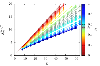
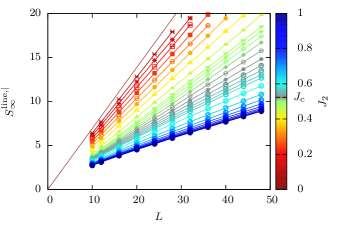
We present in this section our QMC results for the line subsystem SR entropy . Its scaling with the length of the line will be shown to also capture the nature of the ordered and paramagnetic phases. is equal to (minus) the natural logarithm of the maximum diagonal entry of the line reduced density matrix, which turns out to correspond to the two local Néel states and on the line. This is slightly less obvious than the fact that the full Néel states are the most probable states on the full lattice, but we checked explicitly that this is the case in all our simulations. By definition of the reduced density matrix, contains now information about all basis states of the full system which fulfill the geometrical condition of forming one of the two Néel states on the subsystem.
We display our results for the line subsystem SR entropies as a function of the length of the subsystem for both dimerized and plaquettized models in Fig. 4. Much larger system sizes are accessible now (when compared to Fig. 2 for the full system): this greatly reduces the effect of further finite size corrections beyond Eqs. (6) and (7) and makes a reasonable analysis of the scaling of subsystem entropies viable. We now discuss systematically the scaling behavior of the SR entropy across the plaquettization-dimerization transitions, by fitting to the functional forms Eq. (6) and (7), and displaying the estimates of fits parameters.
III.2.1 Leading term
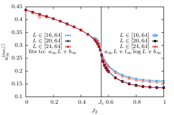
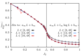
We begin with the linear prefactors , as displayed in Fig. 5 as a function of for fits over different system size windows. The results for the two functional forms are shown in the same figure, but with a different color coding depending on the regimes: obtained from linear fits [Eq. (7)] is represented with bold lines for (in the disordered regime where we find that they represent the correct form) and pale lines for (when they are not expected to be valid) and vice-versa for fits including the logarithmic correction [Eq. (6)]. For , both results agree very well within error bars, while the linear fit result is slightly more stable and converges faster with system size. This is already a hint that the logarithmic correction presumably vanishes in the disordered phase, which will be verified in the next paragraph. Both dimerized and plaquettized models display the same behavior, with taking larger values due to suppressed Néel order.
One can notice a qualitative change in the extensive contribution to the Shannon entropy across the quantum phase transition where changes abruptly. More precisely, its derivative with respect to displays a singularity at the critical point. We discuss in more detail such features in Sec. IV.4.
III.2.2 Subleading logarithmic term in the ordered phase
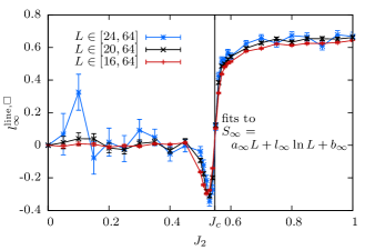
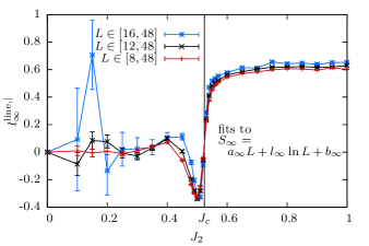
The first subleading scaling term is the logarithmic correction as defined in Eq. (6). Fig. 6 represents results of fits obtained from three sets of system size ranges. We find that fits excluding the smallest system sizes generally correspond to higher fit qualities (quality factor closer to ) while on the other hand, error bars on become larger as the number of data points included in the fit decreases.
Nevertheless, results are stable with respect to different fit windows: we observe a clear change in the estimated exactly at the transition point for both dimerized and plaquettized models at the respective . Deep in the quantum disordered phase, the logarithmic term converges very well towards zero. Close to the critical point for , nontrivial finite size effects show up in pronounced oscillations preceding the jump to nonzero in the ordered phase. Similar to what is observed in the constant term of the SR entropies of the one-dimensional Stéphan et al. (2009) and two-dimensional Luitz et al. (2014) quantum Ising model close to its transition point, the oscillations become narrower and move closer to the critical point with growing system sizes used for the fit. We conclude that in the full disordered phase.
In the ordered phase, the behavior is very different and a logarithmic scaling correction emerges with . Our results for the fitting window with the larger sizes is and appear identical for both models within the Néel phase. However, even though we performed calculations in large systems of up to spins, the asymptotic value of cannot be extrapolated from our data.
Right at the critical point, curves for the estimated for different fit windows cross at a value which is within error bars.
III.2.3 Vanishing constant term in the paramagnetic phase
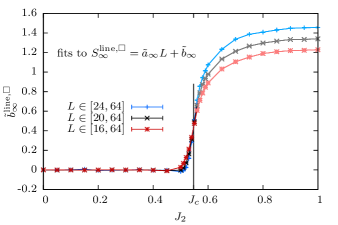
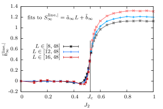
In the quantum disordered phase and presumably also at the critical point, the logarithmic term vanishes and therefore the first subleading scaling term is . To best estimate its value, we force by using the functional form Eq. (7) in our fit. Fig. 7 shows the result of this analysis, the pale lines correspond to the regime where the fit function does not represent the data correctly (this is reflected also by strong finite size effects). We find exactly the same behavior for both models in the disordered phase with for all .
III.2.4 Universal constant term at the quantum phase transition
We furthermore find (see Fig. 7) that curves of for different fit windows cross at the critical point, taking a non-trivial value . The absence of finite size effects at the crossing point provides evidence that the logarithmic correction actually vanishes at the critical point. For the plaquettized model, we find ; in the dimerized case we obtain a similar value . This strongly suggests that is universal at the quantum critical point, and should be identical for all models with a phase transition in the 3d universality class.
To test this, we perform large-scale simulations of the finite-temperature transition in the isotropic 3d Heisenberg model on a cubic lattice with antiferromagnetic interactions. This transition belongs to the 3d universality class. We then computed the line SR entropy using the same QMC technique Luitz et al. (2014), but this time at finite temperature, close to the critical point.
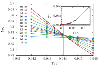
As a preliminary, we want first to extract the best estimate for the critical temperature . We have performed additional simulations, up to sites, studying the crossings of the spin stiffness (times linear system size), a standard method to locate critical points Sandvik (2010). These results are reported in Fig. 8 where we show very precise QMC data for cubic systems, thus allowing to estimate the critical point with a high accuracy to , which agrees with previous estimate from Ref. Yasuda et al., 2005. While measuring the spin stiffness within the SSE computation is very standard Sandvik (2010) and relatively fast, accessing for a single line in the cubic antiferromagnet requires much longer simulation time. We have been able to reach system sizes up to for for which the subleading constant is shown in Fig. 9 in the vicinity of . Despite the sizable error bars, we can nevertheless observe a clear crossing for various fit windows, drifting towards the actual critical point at where the subleading constant takes a numerical value . This value is in perfect agreement with estimates for the two-dimensional quantum critical points, thus reinforcing the evidence for the universality of for 3d O(3) critical points.
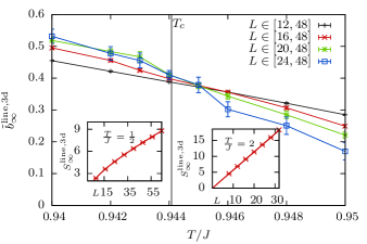
Away from criticality, we have also checked the scalings of in the low temperature ordered phase at (left inset of Fig. 9) and in the high temperature disordered regime at (right inset of Fig. 9). As expected, below , a subleading logarithmic term emerges with , and a purely linear scaling is found above , with a vanishing constant .
IV Participation spectra
Up to now, we have focused on the finite-size behavior of a single quantity, namely (), which is related to a single diagonal element - the largest - of the (reduced) density matrix. Let us now inspect the behavior of all the diagonal elements of the reduced density matrix for a subsystem being, as above, a line of spins embedded in a torus. For practical reasons, we again restrict ourselves to the set of bases that are connected to the basis by global transformations, leaving the Hamiltonian invariant.
IV.1 Definitions
Inspired by recent insights obtained on the entanglement spectrum Li and Haldane (2008); Calabrese and Lefevre (2008); Stéphan et al. (2012), we introduce the participation spectrum obtained from the diagonal of the reduced density matrix in the computational basis
| (8) |
using the line shaped subsystem defined in Fig. 1. From now on, we drop the index ‘line’ on the set of pseudo-energies .
In order to clarify the tremendous amount of information contained in the participation spectrum, we anticipate (as detailed below) that the line participation spectrum will develop well-defined bands that can be classified through specific characteristics of their containing basis states: (absolute value of) magnetization and number of (ferromagnetic) domain-walls , the later turning out to be the crucial element to classify the spectrum.
The operator being diagonal in the computational basis , the magnetization of a basis state is simply defined as . We define the total number of ferromagnetic domain walls in the line as . We assume periodic boundary conditions () along the chain with even (ensuring to be an even number). In other words, is simply the number of bonds along the chain hosting nearest-neighbors spins with the same orientation in basis state . We use the term domain walls since the most likely states are the two Néel states on the chain, as mentioned earlier, which have and (ferromagnetic orientation of spins on a given bond correspond to disrupting local Néel ordering). Magnetization and number of domain walls run from to respectively and (for the polarized ferromagnetic state) for possible basis states on the chain. We expect states with low and low to be more likely, and therefore to have a lower pseudo-energy .

A typical basis state is illustrated in Fig. 10 for a line of 30 spins with and . From such a picture one sees that increasing the separation between two domain walls tends to reduce the total staggered magnetization . It is therefore expected that the effective interaction between domain walls will be strongly (weakly) attractive for states having long-range (short-range) antiferromagnetic correlations. This will be discussed on more quantitative grounds below in Sec. IV.4.
We finally note that this description is not sufficient for characterizing states of the chain subsystem in the plaquettized lattice, as readily seen in Fig. 1. While all bonds along the chain are equivalent for the dimerized lattice, this is not the case for the plaquettized lattice with “strong” bonds carrying the coupling constant and “weak” bonds carrying . We therefore find it useful to define the number of strong domain walls (). We assume that the chain subsystem starts from a strong bond and that is a multiple of , as is the case in Fig. 1. We expect that ferromagnetic domain-walls on strong bonds will be less likely than on weak bonds and anticipate this notion of strong and weak domain walls to be particularly relevant in the quantum disordered phase.
IV.2 Participation density of states
To get a first idea on how the weight of each basis state gets redistributed while passing through the quantum phase transition, it is instructive to consider the density of states
| (9) |
corresponding to the participation spectrum of the line subsystem.
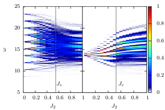
Figure 11 displays the density of states as a function of across the transition in dimerized (right) and plaquettized (left) square lattices. While the two density of states naturally develop into the same homogeneous limit of , they appear to differ strongly for dimerized and plaquettized models, specially in the quantum disordered phase (which is nevertheless physically similar for both models).
This difference is readily understood by considering the limit of (see Appendix B) where the reduced density matrix for isolated plaquettes and dimers is quite different. Indeed, all diagonal elements of the reduced density matrix are equal to for the dimer case, whereas this large degeneracy is lifted by the existence of two different diagonal entries in the reduced density matrix at for a single plaquette. For the plaquettized model, the number of strong domain walls determines the value of the diagonal reduced density matrix element of the line by
| (10) |
and therefore labels the different packets of states at . This degeneracy is lifted at and different packets of states tend apart from their initial pseudo-energy . Due to the high complexity of the spectrum in the plaquettized model, these packets are mixed in energy at the critical point but become “fat” as they cross the critical point. This phenomenon, which will be discussed in detail in Sec. IV.3, is even more visible in the participation spectrum of the dimerized model. There, there is no distinction between strong and weak domain walls, and the well-separated bands evolve smoothly with across the phase transition.
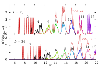
On the other side of the transition, the density of states in the homogeneous limit shows bands of high density in pseudo-energy, separated by local minima. Inspection of the corresponding states confirms our intuition by revealing that the bands can be characterized by the number of domain walls in the basis states. Fig. 12 illustrates this by displaying the density of states for a fixed number of domain walls
| (11) |
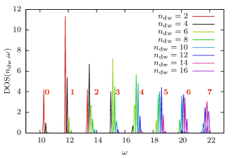
where the sum runs only over states with domain walls. We compare the domain wall resolved density of states for two lattice sizes and in Fig. 12 and it is apparent that the bands seen in Fig. 11 in the ordered phase correspond to states with a fixed number of domain walls. This is in contrast with the gapped phase of the plaquettized model, where the number of strong domain walls is the dominant characteristic for the bands (see Fig. 13). With growing system size, the number of possible bands grows linearly, as the maximal number of domain walls grows linearly in . Also, on the ordered side of the transition the width of the bands grows linearly in (as will be shown in Sec. IV.4) and the bands come closer together, eventually forming a continuum of states.
A similar picture of bands labelled by the number of spin flips has also been proposed for the entanglement spectrum of quantum dimer models on a cylinder Stéphan et al. (2012).
IV.3 Fully-resolved participation spectrum resolution
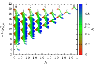
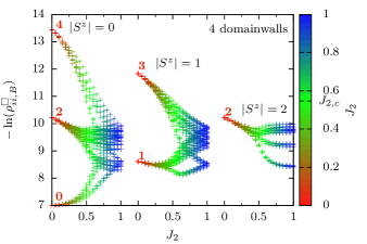
We now turn our attention to the fully resolved participation spectrum for the plaquettization transition, where states are distinguished by . The use of magnetization is mainly for clarity reasons: knowing does not help in resolving bands which are characterized by the number of domain walls (even though some values of magnetization do not accommodate all possible number of domain walls). The splitting of the participation spectrum in different sectors of is displayed in Fig. 14 for different values of for the plaquettized model, illustrating more clearly how the pseudoenergies vary from being grouped by their number of strong domain walls (at ) to their total number of domain walls (at ). A more detailed look at the development of state packets with fixed is provided in Fig 15 where we concentrate on all basis states with exactly domainwalls.
IV.4 Detecting the quantum phase transition in the participation spectrum
While the previous sections aimed at illustrate how participation spectra evolve though the continuous quantum phase transition, we present now two distinct quantitative features for localizing the quantum phase transition in the (fully-resolved) participation spectrum.
IV.4.1 Inflection point
As visible in Figs. 14 and 15, the behavior of the pseudo-energy of each basis state is peculiar close to the quantum critical point, showing a maximal or minimal steepness of and a zero transition of the second derivative , i.e. every shows an inflection point at the critical point. While the change of curvature of close to is clearly visible for most basis states in Figs. 14 and 15, a quantitative demonstration that the inflection point lies right at the critical point requires high accuracy of and a fine grid in . We therefore performed this analysis for for best control.
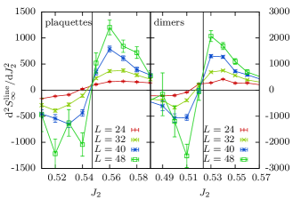
We compute numerically the second derivative of with respect to close to the quantum phase transition and display it in Fig. 16 for both the dimerized and plaquettized models, confirming that the quantum phase transition corresponds to a zero in the second derivative. In the limit , the first derivative of diverges right at the critical point and thus precisely marks the quantum phase transition.
IV.4.2 Finite-size dependence of resolved bands and domain walls confinement
Another way to quantitatively detect the quantum phase transition is obtained following the previous observation that bands of identical number of domain walls in the participation spectra appear to become “fatter” as the system crosses the quantum critical point.
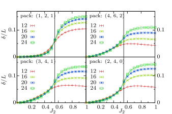
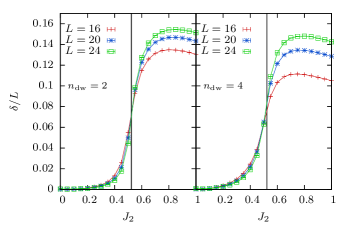
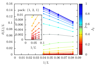
We investigate the size of state packets labeled by in the plaquettized case by looking at the difference in pseudo-energy between the basis states with the largest and lowest pseudo-energy within the packet . Results for the normalized packet width for different (see top panel of Fig. 17) display a clear crossing point at the quantum critical point, separating two different regimes. In the quantum disordered phase, the normalized packet width tends to vanish presumably as in the thermodynamic limit, as revealed by the finite-size scaling analysis in the inset of Fig. 18. On the other hand, the packet width grows as (with correction) in the ordered phase as also seen in Fig. 18. The same behavior is revealed when integrating over all sectors as shown for the case of the dimerized model in the bottom panel of Fig. 17, where state packets are defined by a fixed number of domain walls .
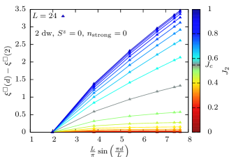
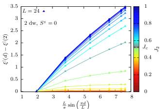
This behavior can be understood following the sketch presented in Fig. 10, where one sees that the dynamics of two domain walls is constrained by the relative sizes of two Néel patterns, and . Since the staggered magnetization of a single basis state depends on the size difference between Néel domains of different type, one can predict a qualitative difference for the packet width between ordered and disordered ground states. In the disordered phase where antiferromagnetic correlations are short-ranged, we naturally expect that the pseudo-energies will not be affected (remaining essentially constant) when the separation between two domain walls becomes larger than the finite correlation length. On the other hand, for long-range order a confinement mechanism between two domain walls will be necessary to maintain a finite staggered magnetization. There we expect the pseudo-energy spectrum to be controlled by an attractive long-range interaction between domain walls. This picture holds best for a small number of domain walls in the high probability (low pseudo-energy) part of the participation spectrum.
We illustrate this interpretation by considering the pseudo-energy dependence on the distance between domain walls. Fig. 19 displays this pseudo-energy difference for the diluted case of domain-walls with (in which case the distance has to be even), as a function of the chord distance between domain walls for different for both dimerized and plaquettized models. In the disordered phase, the domain walls appear rapidly deconfined with a finite small pseudo-energy difference between states with different domain wall distances and hence a small packet width . In contrast, large domain wall distances are penalized in the magnetically ordered phase by a high pseudo-energy cost, which appears to grow approximatively linearly with distance (for a large enough distance).
For states with more than two domain walls, the situation becomes somewhat more complicated. The crossing in still exists but it acquires a drift with system size (see Fig. 17). A closer inspection of the involved states in the corresponding packet and their pseudo-energies suggests that multi-domain wall attraction terms play a role in addition to the long-range domain-walls attraction. This is probably the source of the a drift of the crossing as these multi-domain wall terms become eventually less important when the average distance between domain walls becomes large for the high end (low probability) of a packet with a fixed number of domain walls.
V Conclusion
We have analyzed the Néel antiferromagnet-paramagnet quantum phase transition in two-dimensional quantum spin systems using the Shannon-Rényi entropies for the full system and for subsystems, together with the associated participation spectra, using extensively QMC methods presented in Ref. Luitz et al., 2014. Our study shows that a line shaped one-dimensional subsystem is actually sufficient to capture the quantum phase transition. We confirm that the subleading scaling behavior of Shannon-Rényi entropies changes radically at the quantum phase transition, giving rise to a logarithmic scaling term in the Néel phase, independent on microscopic details (such as the choice of dimerization or plaquettization of the lattice in our study).
Similar logarithmic corrections to an area law have been numerically observedKallin et al. (2011); Humeniuk and Roscilde (2012); Ju et al. (2012) in studies of the Rényi entanglement entropy of the ground-state of the 2d Heisenberg model for two-dimensional subsystems (such as half-torus), in agreement with theoretical predictions Metlitski and Grover (2011). For the case of a line-shaped subsystem, we have checked that the Rényi entanglement entropy also exhibits a logarithmic correction to the area law (indistinguishable from a volume law in this particular case).
On the disordered side of the phase diagram, only a subleading constant term can be present, which is actually in this phase with no broken symmetry.
At the quantum critical point, we find a universal subleading constant (for the line SR entropy ) with an estimated value of being identical for dimerized and plaquettized models. We have confirmed that a similar constant can be found at the Néel-paramagnetic finite-temperature phase transition of the 3d Heisenberg antiferromagnet at , strongly suggesting that this is a characteristic of the 3d universality class to which all mentioned transitions belong. We suspect that such a universal subleading constant also exists for the SR entropy of the full system, but the precision of our numerical computations do not allow to prove this. Universality could be further checked by considering critical points in other models, either with two-dimensional quantum models such as bilayers Sandvik and Scalapino (1994), coupled Haldane chains Sakai and Takahashi (1989); Matsumoto et al. (2001), staggered-dimer models where anomalously large corrections to scaling are known Fritz et al. (2011), or in 3d classical systems such as the classical Heisenberg model on the cubic lattice. It would also be very interesting to extend this study to other universality classes, either of conventional or unconventional type Senthil et al. (2004).
Motivated by the finding that the one-dimensional subsystem captures the physics of the phase transition, we also performed a phenomenological study of the information contained in the participation spectra of the subsystem. In the participation spectra, states group together in packets of pseudo-energy which can be classified by the number of ferromagnetic domain walls (number of strong domain walls for the plaquettized lattice) in the basis states. The development of these packets across the transition is peculiar as packets become “fat” in the ordered phase, meaning that their width (in pseudo-energy) grows linearly with subsystem size . In the disordered phase, however, tends to zero. This can be phenomenologically explained by an attractive potential between domain walls in the ordered phase, while in the disordered phase, domain walls remain deconfined. In addition, we observe at the critical point an interesting behavior for the pseudo-energies in the participation spectrum: their slope as a function of the control parameter has a pronounced extremum and we show that has an inflection point at .
The analysis presented in Sec. IV is fairly simple, but contains the basic ingredients to build a wave-function that describes the studied (2+1)-dimensional quantum phase transition. Let us indeed put in perspective our work with the widely-used variational approach. In the context of two-dimensional Heisenberg models, Huse and Elser Huse and Elser (1988) (see also Refs. Manousakis, 1989; Liu and Manousakis, 1989) formulated a variational ansatz for the ground-state wave function:
| (12) |
where a classical pseudo-energy is associated to the basis state (also taken as a basis state in Ref. Huse and Elser, 1988). Here is (a set of) variational parameter(s) used to minimize the total energy of the Heisenberg Hamiltonian. This ansatz looks similar to our definition of the participation spectrum. The crucial difference is of course that the variational approach assumes a form for the pseudo-energy (for instance a power-law Ising interaction in Ref. Huse and Elser, 1988), while our QMC methods can calculate the exact (within statistical accuracy) value of each . Note as well that we did not compute, for essentially practical reasons, the participation spectrum for the full system (as in the variational ansatz) but rather on a subsystem. Nevertheless, our results give the correct qualitative ingredients to construct variational wave-functions of the form of Eq. (12) to describe the Néel and paramagnetic phases, as well as the transition in between. This could be useful in particular for frustrated spin systems, where QMC is not available.
Acknowledgements.
We would like to thank F. Assaad, F. Bègue, G. Misguich, G. Roux, S. Pujari and J.-M. Stéphan for many useful discussions, as well as G. Misguich, M. Oshikawa and X. Plat for collaboration on related topics. Our QMC codes are partly based on the ALPS libraries Bauer et al. (2011). This work was performed using numerical resources from GENCI (grants 2013-x2012050225 and 2014-x2013050225) and CALMIP and is supported by the French ANR program ANR-11-IS04-005-01.Appendix A Details on Monte Carlo procedure
Here we provide further details (in supplement to Ref. Luitz et al., 2014) on the QMC procedure to access subsystem entropies and participation probabilities, as well as on dealing with statistical uncertainty.
A.1 Calculation of diagonal elements of the reduced density matrix
As already presented in Ref. Luitz et al., 2014, the diagonal elements of the full density matrix are readily available in standard QMC techniques such as the standard stochastic series expansion method (cf. e.g. Ref. Sandvik, 2010). In the same vein, the diagonal elements of the reduced density matrix (see Eq. (2)) are obtained in the following way. It is clear that the probability of observing the basis state in the SSE operator string is directly given by
| (13) |
Hence, the probability of finding the subsystem basis state in subsystem in the stochastic series expansion operator string is
| (14) |
In practice, this means that one has to inspect only the -part of each basis state in the simulation, and record a histogram of its frequency.
A.2 Computationally accessible entropies
The numerical calculation of large SR entropies corresponds to the observation of rare events with low probabilities. It is easy to obtain an approximation of a reasonable upper limit for the calculation of the entropy given by the observation of the most probable state appearing in the SSE Markov chain with a probability . For the estimation of the maximally accessible entropy, we make the assumption of statistical independence, as statistical correlations will only reduce the maximally accessible entropy.
In the Markov chain, we measure the observable , yielding of state corresponds to the state with maximal probability and otherwise. The Monte Carlo average of this observable is given by
| (15) |
where is the number of occurrences of the most probable state in the Markov chain MC of length 111Note that in the case of SSE, the effective length of the Markov chain is rather the number of operator strings times the expansion order . .
The standard error of is given by
| (16) |
for sufficiently small and inspected states. Now we can estimate the standard error of by the linear approximation . To obtain a given relative error for a given number of inspected states, the maximal entropy is then governed by the equation:
| (17) |
In a realistic calculation, we inspect typically states. Therefore, for a requirement of a relative error , we obtain a maximally accessible entropy .
A.3 Error bars for the participation spectrum
Measuring accuracy on the participation spectrum requires special care. It is indeed impractical to construct an observable for each subsystem basis state and measure as proposed in Ref. Luitz et al., 2014 for each observed state in the SSE operator string. For the calculation of the participation spectrum, defined as and inducing a nonlinear transformation of the Monte Carlo data, we perform several independent Monte Carlo simulations in parallel, each creating a simple histogram containing the count of all observed subsystem basis states. After applying all model symmetries to the histogram to improve the statistics (see supplementary material of Ref. Luitz et al., 2014), we perform a bootstrap analysis for each , creating bootstrap samples from the histogram counts of the different independent simulations. This provides an unbiased estimation of the standard errors of the mean of all .
Appendix B Exact calculations for
We provide here simple exact results for SR entropies and reduced density matrices when . These results are useful in two ways: they provide direct insight for the subleading terms of the SR entropies (which vanish altogether when ) as well as on the starting point of the participation spectrum.
B.1 Shannon Rényi entropy of the full system
In the limit of isolated plaquettes or dimers, the groundstate is a singlet state, given by
| (18) |
for one plaquette (see e.g. Ref. Ueda and Totsuka, 2007)) and
| (19) |
for a single dimer.
Thus, we get
| (20) |
and
| (21) |
for the limit of the plaquettized model.
The solution is much simpler for the dimerized model, as any basis state with on the dimer contributes with the same weight and therefore all SR entropies are identical:
| (22) |
B.2 Shannon Rényi entropy of the line sub-system
For a dimer shaped subsystem of one plaquette, the reduced density matrix is given (in the basis) by
| (23) |
In the single dimer case, subsystem is just one site and the reduced density matrix (in the basis) is
| (24) |
The total reduced density matrix of the line shaped subsystem composed of dimers of single plaquettes (or sites of single dimers in the dimerized case) is then obtained from the Kronecker product of the reduced density matrices:
| (25) |
Consequently, for the line shaped subsystem, reduces to
| (26) |
While for arbitrary values of , the Shannon-Rényi entropies are
| (27) |
References
- Wegner (1980) F. Wegner, Zeitschrift für Physik B Condensed Matter 36, 209 (1980).
- Fyodorov and Mirlin (1992) Y. V. Fyodorov and A. D. Mirlin, Phys. Rev. Lett. 69, 1093 (1992).
- Evers and Mirlin (2000) F. Evers and A. D. Mirlin, Phys. Rev. Lett. 84, 3690 (2000).
- Evers and Mirlin (2008) F. Evers and A. D. Mirlin, Rev. Mod. Phys. 80, 1355 (2008).
- Stéphan et al. (2009) J.-M. Stéphan, S. Furukawa, G. Misguich, and V. Pasquier, Phys. Rev. B 80, 184421 (2009).
- Stéphan et al. (2010) J.-M. Stéphan, G. Misguich, and V. Pasquier, Phys. Rev. B 82, 125455 (2010).
- Stéphan et al. (2011) J.-M. Stéphan, G. Misguich, and V. Pasquier, Phys. Rev. B 84, 195128 (2011).
- Zaletel et al. (2011) M. P. Zaletel, J. H. Bardarson, and J. E. Moore, Phys. Rev. Lett. 107, 020402 (2011).
- Luitz et al. (2014) D. J. Luitz, F. Alet, and N. Laflorencie, Phys. Rev. Lett. 112, 057203 (2014).
- Atas and Bogomolny (2012) Y. Y. Atas and E. Bogomolny, Phys. Rev. E 86, 021104 (2012).
- Um et al. (2012) J. Um, H. Park, and H. Hinrichsen, Journal of Statistical Mechanics: Theory and Experiment 2012, P10026 (2012).
- Alcaraz and Rajabpour (2013) F. C. Alcaraz and M. A. Rajabpour, Phys. Rev. Lett. 111, 017201 (2013).
- Troyer et al. (1997) M. Troyer, M. Imada, and K. Ueda, J. Phys. Soc. Jpn. 66, 2957 (1997).
- Matsumoto et al. (2001) M. Matsumoto, C. Yasuda, S. Todo, and H. Takayama, Phys. Rev. B 65, 014407 (2001).
- Wang et al. (2006) L. Wang, K. S. D. Beach, and A. W. Sandvik, Phys. Rev. B 73, 014431 (2006).
- Albuquerque et al. (2008) A. F. Albuquerque, M. Troyer, and J. Oitmaa, Phys. Rev. B 78, 132402 (2008).
- Wenzel and Janke (2009) S. Wenzel and W. Janke, Phys. Rev. B 79, 014410 (2009).
- Sandvik (2010) A. W. Sandvik, AIP Conference Proceedings 1297, 135 (2010).
- Yasuda et al. (2005) C. Yasuda, S. Todo, K. Hukushima, F. Alet, M. Keller, M. Troyer, and H. Takayama, Phys. Rev. Lett. 94, 217201 (2005).
- Li and Haldane (2008) H. Li and F. D. M. Haldane, Phys. Rev. Lett. 101, 010504 (2008).
- Calabrese and Lefevre (2008) P. Calabrese and A. Lefevre, Phys. Rev. A 78, 032329 (2008).
- Young (2012) P. Young, “Everything you wanted to know about data analysis and fitting but were afraid to ask,” (2012), arXiv:1210.3781 .
- Stéphan et al. (2012) J.-M. Stéphan, G. Misguich, and V. Pasquier, Journal of Statistical Mechanics: Theory and Experiment 2012, P02003 (2012).
- Kallin et al. (2011) A. B. Kallin, M. B. Hastings, R. G. Melko, and R. R. P. Singh, Physical Review B 84, 165134 (2011).
- Humeniuk and Roscilde (2012) S. Humeniuk and T. Roscilde, Physical Review B 86, 235116 (2012).
- Ju et al. (2012) H. Ju, A. B. Kallin, P. Fendley, M. B. Hastings, and R. G. Melko, Physical Review B 85, 165121 (2012).
- Metlitski and Grover (2011) M. A. Metlitski and T. Grover, arXiv:1112.5166 [cond-mat, physics:hep-th, physics:quant-ph] (2011).
- Sandvik and Scalapino (1994) A. W. Sandvik and D. J. Scalapino, Phys. Rev. Lett. 72, 2777 (1994).
- Sakai and Takahashi (1989) T. Sakai and M. Takahashi, J. Phys. Soc. Jpn. 58, 3131 (1989).
- Fritz et al. (2011) L. Fritz, R. L. Doretto, S. Wessel, S. Wenzel, S. Burdin, and M. Vojta, Phys. Rev. B 83, 174416 (2011).
- Senthil et al. (2004) T. Senthil, A. Vishwanath, L. Balents, S. Sachdev, and M. P. A. Fisher, Science 303, 1490 (2004).
- Huse and Elser (1988) D. A. Huse and V. Elser, Phys. Rev. Lett. 60, 2531 (1988).
- Manousakis (1989) E. Manousakis, Phys. Rev. B 40, 4904 (1989).
- Liu and Manousakis (1989) Z. Liu and E. Manousakis, Phys. Rev. B 40, 11437 (1989).
- Bauer et al. (2011) B. Bauer, L. D. Carr, H. G. Evertz, A. Feiguin, J. Freire, S. Fuchs, L. Gamper, J. Gukelberger, E. Gull, S. Guertler, A. Hehn, R. Igarashi, S. V. Isakov, D. Koop, P. N. Ma, P. Mates, H. Matsuo, O. Parcollet, G. Pawłowski, J. D. Picon, L. Pollet, E. Santos, V. W. Scarola, U. Schollwöck, C. Silva, B. Surer, S. Todo, S. Trebst, M. Troyer, M. L. Wall, P. Werner, and S. Wessel, Journal of Statistical Mechanics: Theory and Experiment 2011, P05001 (2011).
- Note (1) Note that in the case of SSE, the effective length of the Markov chain is rather the number of operator strings times the expansion order .
- Ueda and Totsuka (2007) H. T. Ueda and K. Totsuka, Phys. Rev. B 76, 214428 (2007).