An accurate and efficient Lagrangian sub-grid model

Abstract

A computationally efficient model is introduced to account for the sub-grid scale velocities of tracer particles dispersed in statistically homogeneous and isotropic turbulent flows. The model embeds the multi-scale nature of turbulent temporal and spatial correlations, that are essential to reproduce multi-particle dispersion. It is capable to describe the Lagrangian diffusion and dispersion of temporally and spatially correlated clouds of particles. Although the model neglects intermittent corrections, we show that pair and tetrad dispersion results nicely compare with Direct Numerical Simulations of statistically isotropic and homogeneous $3D$ turbulence. This is in agreement with recent observations that deviations from self-similar pair dispersion statistics are rare events.

I Introduction

The transport of particles in turbulent flows is strongly sensitive to the multi-scale and multi-time fluctuactions of the turbulent Eulerian velocity. For this reason, the dispersion of particles poses extraordinary challenges when the complexity of the flow geometry or the large Reynolds numbers requires the use of turbulence models. In particular, the modelisation of the small Eulerian scales can significantly alter the dynamics of particle dispersion. Particle dispersion in turbulence, either from extended or from localized sources Silv2010 ; SBTPRL2012 , is a very common phenomenon of practical importance for atmospheric as well as for many applied problems toschi_bode . Among the many possible examples, we remind here the dynamics and the spatial distribution of pollutants and pollen in the atmosphere MH2006 ; CM2011 ; LMR2008 ; ML2012 or oceanic flows berti2011 ; Palatella2013 , the formation and the dynamics of small rain droplets in clouds shaw2003 , the dynamics of colloidal aggregates in turbulence BMB2008 ; BBL2012 , the combustion of fuel droplets and the formation of soot particles in engines PA2002 .

The development of turbulence models and closures, to describe the effect of the unresolved or sub-grid scale (SGS) features of the Eulerian vector or scalar fields, has a long history dating back to Lilly and Smagorinsky (see segaut ). It is fair to say that nowadays there are a number of well-established classical SGS models for homogeneous and isotropic turbulence (HIT), adapted and extensively tested under a variety of conditions MK2000 , as well as more recent proposals keeping into account the phenomenology of turbulence beyond HIT (see e.g., MoengSullivan ; ToschiLeve ).
The development of sub-grid models for Lagrangian turbulence has a relatively shorter history, partly due to the lack of accurate experimental and direct-numerical simulation measurements of Lagrangian statistics in high-Reynolds number flows. The recent availability of a large amount of Lagrangian statistics measurements in HIT Ott ; Xunature ; PintonPRL ; IK2002 ; YeBo2004 ; BoffSok3D ; PRL2004 ; Pof2005 has allowed to quantitatively establish the phenomenological picture for tracers (reviewed in Yeungrev ; Sawfordrev ; Collinsrev ), and partially also for inertial point-particles JFM2010 . The knowledge borrowed from experiments and direct numerical simulations has then promoted new research on Lagrangian sub-grid scale models for tracers, and inertial particles also (see e.g., Weil2004 ; LMR2008 ; JH2013 ). The effects of small-scale temporal and spatial correlations on the dynamics of particles are an important problem FGVrev . In particular beyond classical measurements of the Lagrangian dynamics of a single particle and of particle pairs, the geometric features of multiparticles dispersion has also been investigated CPS99 ; Pof2005multi ; Xu2007 ; HYS2011 .
Within the complex picture of Lagrangian dynamics, one of the most important point is that Lagrangian turbulence is more intermittent than Eulerian turbulence PRLall and, as a result, one may have to pay additional care when using Gaussian models to model the Lagrangian velocity fields. Moreover, in HIT, the relative dispersion of tracers is mainly dominated by small-scale fluid motions: if these are neglected, particle pairs disperse at a much slower rate than the actual one (ballistic vs Richardson dispersion).

Traditionally, Lagrangian SGS motions are described by means of stochastic models. These are based on stochastic differential equations for the evolution of the velocity, assumed to be Markovian, along a particle trajectory. These can be built up for single particle trajectories Tho87 , two-particle KD88 ; Tho90 ; K97 and four-particle dispersion DevTho2013 ; Dev2013 . The literature on the topic is vast and we cannot review it here. What is important for the present discussion is that stochastic models for two-particle dispersion are generally inconsistent with single particle statistics, so that depending on the problem at hand one has to change model.
A different approach was developed in Lacorata et al. LMR2008 , where a multiscale kinematic velocity field was introduced to model turbulent relative dispersion at sub-grid scales. The authors exploited Lagrangian chaotic mixing generated by a nonlinear deterministic function, periodic in space and time. This approach differs from kinematic models (e.g. Fung1992 ; FV1998 ), as it reproduces the effect of large-scale sweeping on particle trajectories Chaves ; DevThom2005 ; Eyinksweep .
In the context of wall-bounded flows, Lagrangian SGS schemes have been proposed in terms of approximate deconvolution models based on the Eulerian field (see e.g., K2006 ), or in terms of force-based models soldati_salvetti . Observables capable to discriminate between model error and drift induced errors were proposed toschi_donini .
Most of these models rely on the knowledge of the resolved Eulerian velocity field, however we note that models to solve the Lagrangian dynamics self-consistently without an underlying Eulerian velocity field have been proposed. This is for example the idea behind Smoothed Particle Hydrodynamics (SPH), i.e. a purely Lagrangian scheme to solve the Navier-Stokes equation, recently reviewed in Mon2012 . In Smoothed Particle Hydrodynamics, instead of solving the fluid equations on a grid, it is used a set of particles, whose equations of motion are determined from the continuum Navier-Stokes equations.

An important issue concerns the possibility to build up models accounting for multi-particle dispersion, ${\cal N}>2$, going beyond the pair separation dynamics. Multi-particle Lagrangian models invariably need to incorporate a mechanism correlating the sub-grid-scale velocities of the particles. Different approaches are possible. In Sawford et al. Sawford2013 , a two-particle stochastic model for $3D$ Gaussian turbulence Tho90 ; bor94 has been generalised to the problem of $n$ tracers: these are constrained by pair-wise spatial correlations, implying that multi-point correlations are neglected. Interestingly, the model shows a good agreement of multi-point statistics with direct numerical simulations results. Alternatively, Burgener et al. Burgener2012 proposed to build spatial correlations between the fluid particles by minimasing of a Heisenberg-like Hamiltonian. In the Hamiltonian, the two-object coupling function is distance dependent and with a power law behaviour. Ballistic separation and Taylor diffusion regimes in pair dispersion are clearly observed, while turbulent inertial-range dispersion á la Richardson is observed in specific conditions.

In this manuscript we introduce a novel, accurate and computationally efficient Lagrangian Sub-Grid Scale model (LSGS) for the dispersion of an arbitrary number of tracers in $3D$ statistically homogeneous and isotropic turbulent flows. The model is purely Lagrangian and it defines and evolves the velocities of tracers at their positions. The trajectories of ${\cal N}$ particles are simply obtained by time-integrating the Lagrangian velocities. It is primarily meant to reproduce Lagrangian dispersion as sub-grid scales, but it may be used as well as a rudimental Lagrangian Navier-Stokes solver, much in the spirit of SPH.
The model encodes velocity fluctuations that scale in space and in time consistently with Kolmogorov 1941 frisch , hence without intermittentcy corrections, and is self-consistent for an arbitrary number or density of tracers. An essential prescription for the model is the capability to correctly reproduce single-particle absolute diffusion together with multi-particle dispersion. For the latter, we require proper reproduction of inertial range pair dispersion (Richardson dispersion Sawfordrev ; Pof2005 ; Collinsrev ), as well as dynamics and deformation of tetrads.
In a nutshell, the idea of our LSGS model is to define a multiscale relative velocity difference between two tracers, consistent with Kolmogorov inertial range scaling. Such velocity difference, characterized by the proper eddy turnover time, is able to reproduce Richardson dispersion for a single pair of tracers. The model is built up in a similar spirit of what done in LMR2008 for tracer pair dispersion, but it is capable of ensuring consistent correlations between an arbitrary number of tracers according to their positions and relative distances. Space correlations ensure that tracers close in space will experience very similar SGS velocities. Beyond pair dispersion, we also quantitatively validate the temporal evolution and dispersion properties of groups of four particles (tetrads), against Direct Numerical Simulations results Pof2005multi .

The paper is organized as follows. In Section II, we introduce the LSGS model for an arbitrary number of tracers, and with an arbitrary large inertial range of scales. In Sec. III, we specify the model parameters and discuss the results for absolute, pair and tetrad dispersion. Last section is devoted to concluding remarks.

II The Lagrangian Particle Model

In large-eddy simulations, the full tracer velocity is defined as the sum of the resolved Lagrangian velocity component, ${\bm{V}}_{i}({\bm{x}}_{i},t)$, and the sub-grid-scale contribution, ${\bm{v}}_{i}({\bm{x}}_{i}(t),t)$. The larger scale components of the velocity, characterized by larger correlation times, sweep the smaller ones thus advecting both particles and small-scale eddies. This is a crucial feature of Lagrangian turbulence, sometimes neglected in synthetic models of Eulerian turbulence, that incorrectly describe pair dispersion Chaves ; DevThom2005 ; Eyinksweep .
The Lagrangian sub-grid-scale model describes the $3D$ velocity, ${\bm{v}}_{i}({\bm{x}}_{i}(t),t)$, at the position, ${\bm{x}}_{i}(t)$, of the $i-$th of the ${\cal N}$ tracer particles. The velocity fluctuations along each particle trajectory are the superposition of different contributions from eddies of different sizes. These eddies constitute a turbulent field, decomposed for convenience in terms of logarithmically spaced shells.
We consider the velocity of a tracer built as the sum of a set of fluctuations, ${\bm{u}}_{n}$, of index $n$ associated to a equispaced set of lengthscales, $l_{n}$. Given the largest length scale of the flow, $L_{0}$, smaller scales are defined as:

$$l_{n}=\frac{L_{0}}{\lambda^{n}},\,\quad\quad n=0,\dots,N_{m}-1\,,$$ (1)

where $N_{m}$ is the total number of modes, scales are logaritmically equispaced and the factor $\lambda>1$ is conventionally chosen as $\lambda=2^{1/4}$. Length-scales correspond to wave-numbers $k_{n}\,=\,2\pi/l_{n}$, so that the velocity amplitudes and the associated turn-over times are defined as

$$u_{n}=q_{0}\,k_{n}^{-1/3},\qquad\tau_{n}=l_{n}/u_{n}\,,$$ (2)

where $q_{0}$ is associated with the amplitude of the large-scale velocity.

II.1 Implementation of the LSGS

With the aim of making the description as clear as possible, we consider that the model is best illustrated by the following two-steps procedure:
Step 1: At time $t$ the positions ${\bf x}_{i}(t)$ of all ${\cal N}$ particles are given. The algorithm then generates -for each tracer $i$ and for each lengthscale $l_{n}$- a first set of velocity vectors $\bm{\zeta}_{n}^{(i)}(t)$ (the three velocity components along the space directions $x,y,z$ that are chosen independently from each other). Each of these velocities is the outcome of an Ornstein-Uhlenbeck (OU) process with correlation time $\tau_{n}=l_{n}/u_{n}$ and variance $u_{n}^{2}$, at the scale $l_{n}$. The time evolution of the OU process, for each spatial component of the velocity field of the $i-$th particle at lengthscale $l_{n}$, is obtained according to gil96

$$\zeta_{n}^{(i)}(t+dt)\,=\,\zeta_{n}^{(i)}(t)\,e^{-dt/\tau_{n}}+u_{n}\sqrt{1\,-\,e^{-2dt/\tau_{n}}}\,g\,,$$ (3)

where, for simplicity, we have omitted the sub-script for the spatial components. In (3), the variable $g$ is a random number, normally distributed in the range $[0;1]$. According to our definitions, each OU process is a normally distributed, random variable, $\zeta_{n}^{(i)}(t)$, whose mean value $\mu_{n}^{(i)}$ and standard deviation $\sigma_{n}^{(i)}$ are :

$$\mu_{n}^{(i)} = \zeta_{n_{0}}\,\exp{\left[-(t-t_{0})/\tau_{n}\right]}\,$$ (4)

$$\sigma_{n}^{(i)} = u_{n}\,\sqrt{1-\exp{\left[-2(t-t_{0})/\tau_{n}\right]}}.$$ (5)

The equilibrium time $O(\tau_{0})$ is needed for each mode to relax to a zero mean velocity and to the variance $u_{n}^{2}$. The velocity associated to the $i-$th tracer particle is the superposition of $N_{m}$ modes given by

$${\bf v}^{(i)}(t)=\sum_{n=0}^{N_{m}-1}\bm{\zeta}_{n}^{(i)}(t)\,.$$ (6)

So doing, each particle has a multiscale, single-point velocity field which has the physical time correlations, but which does not respect space correlations yet. Indeed, based on the above algorithm, very different velocity fields could be assigned to particles residing in very close spatial position.

Figure 1: A sketch of the model. The sketch is for the case of three particles (${\bf a}$, ${\bf b}$ and ${\bf c}$) with velocity fields composed by three eddies ($1$, $2$ and $3$, that corresponds to the three circles of diameter, respectively, $l_{1}$, $l_{2}$ and $l_{3}$). Tracers positions are indicated by black dots, while dashed circles are correlation radii relative to the eddies with diameter $l_{1}$, $l_{2}$ and $l_{3}$ (corresponding to shells 1,2, and 3). The largest eddy described by the sub-grid-scale model may correspond to the smallest resolved eddy of the Eulerian Large-eddy simulation. In case of a purely Lagrangian evolution, i.e. without a large-scale model or a LES, the largest eddy corresponds to the integral scales of the system, $L_{0}$. The three modes of the velocity of particle “${\bf a}$” are computed by modulating the OU processes associated to particle “${\bf a}$”, - $\bm{\zeta}_{i}^{({\bf a})}$ with $i=1,2,3$ -, with the OU processes attached to particles “${\bf b}$” and “${\bf c}$”. This is done, in this simple example, according to: ${\bf v}_{1}^{({\bf a})}=\bm{\zeta}_{1}^{({\bf a})}+\bm{\zeta}_{1}^{({\bf b})}(1-{r_{ab}\over l_{1}})+\bm{\zeta}_{1}^{({\bf c})}(1-{r_{ac}\over l_{1}})$; ${\bf v}_{2}^{({\bf a})}=\bm{\zeta}_{2}^{({\bf a})}+\bm{\zeta}_{2}^{({\bf b})}(1-{r_{ab}\over l_{2}})$; ${\bf v}_{3}^{({\bf a})}=\bm{\zeta}_{3}^{({\bf a})}$, where we have kept into account the fact that (a) and (b) overlap with shells 1 and 2, while (a) and (c) overlap only with shell 1.

Step 2: In order to build up the proper spatial correlations and establish a correspondence between the modelled particle velocities and the two-point Eulerian statistics, we redefine for the $i-th$ particle the fluctuation associated to the $n$-th mode as follows ,

$${\bf v}_{n}^{(i)}(t)=\sum_{j=1}^{{\cal N}}\bm{\zeta}_{n}^{(j)}(t)\cdot\left(1-f_{l_{n}}(|{\bf x}_{i}-{\bf x}_{j}|)\right)\,.$$ (7)

Here the decorrelation function is such that $f(r)\propto r$ for $r\ll 1$ and $f(r)\simeq 1$ for $r\gg 1$. Note that in (7), the $n-th$ mode velocity fluctuation for the $i-$th particle is determined by the value of the $n-th$ mode velocity fluctuation of the particle $j$, with $j=1,\dots,{\cal N}$ spanning over the entire particle ensemble. Clearly, only particles closeby matter, while particles located very far from $i$ will not matter.

The particle velocity resulting from the contributions of different eddies is then evaluated as:

$${\bf v}^{(i)}(t)=\sum_{n=0}^{N_{m}-1}\frac{1}{{\cal A}_{n}^{(i)}}{\bf v}_{n}^{(i)}(t).$$ (8)

The normalization factor that preserves the variance is given by

$${\cal A}_{n}^{(i)}=\sqrt{\sum_{j=1}^{\cal N}(1-f_{l_{n}}(|{\bf x}_{i}-{\bf x}_{j}|))^{2}}.$$ (9)

As a result of this procedure, space correlations are introduced among the velocities of the whole particle ensemble. Particle velocities are no longer statistically independent, but behave as responding to the same local eddy fluctuations. In Figure 1, a graphic sketch of the model is given for the case of three Lagrangian tracers, with a few modes velocity.

Note that, from (6), the variance of each velocity component along $x,y,z$ is:

$$\langle{v^{\prime}}^{(i)}(t)^{2}\rangle=\sum_{n=0}^{N_{m}-1}\langle{\bf\zeta}_{n}^{(i)}(t)^{2}\rangle\,,$$ (10)

since modes are independent, $\langle{\bf\zeta}_{n}^{(i)}(t){\bf\zeta}_{n^{\prime}}^{(i)}(t)\rangle=0$ for $n\neq n^{\prime}$. If by physical arguments, we require a velocity field with root-mean-square values to $v_{rms}=u_{0}$, it is enough to introduce in the velocity definition given in equation (6) or equation(8), the norm ${\cal F}$ defined as ,

$${\cal F}^{2}=\frac{u_{0}^{2}}{\sum_{n=0}^{N_{m}-1}u_{n}^{2}}\,.$$ (11)

It is worth mentioning that the model has a tunable free parameter, corresponding to the turbulent energy dissipation rate. If used as a sub-grid, such parameter is provided by the large-scale model (e.g., a large-eddy simulation), and can then be used to fix the ratio among large-scale velocity and length values. In the absence of a large-scale model, an energy dissipation rate can be fixed up to constant $O(1)$.

We note that from a computational point of view, the simplest implementeation of the LSGS model scales as ${\cal N}^{2}$, but it can be easily optimized with standard Molecular Dynamics algorithms (e.g. by using a linked list).
To validate the model against observations for statistically homogeneous and isotropic $3D$ Lagrangian turbulence, we consider in the following the most challenging case corresponding to ${\bm{V}}=0$, when the sub-grid-scale model is solely responsible for the dynamics of tracers at all scales. Thus, to simplify the text, from now on the term “sub-grid” is dropped and we speak of tracers velocities; moreover we adopt the shorthand notation ${\bm{v}}_{i}(t)\equiv{\bm{v}}_{i}({\bm{x}}_{i}(t),t)$.
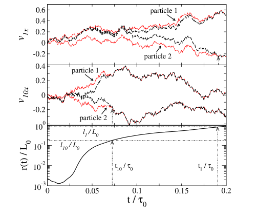
A first glance on the behaviour of the model can be appreciated in Figure 2. Here we consider the results of a simulation with only a pair of particles, with relative distance $r_{0}$ smaller than the smallest eddy $l_{N_{m}-1}$ of the velocity field. Simulation parameters are summarized in Table 1, case $N_{m}=31$. For plotting purpose, we selected two modes, namely mode $n=1$ of length scale $l_{1}=L_{0}/\lambda$ and mode $n=10$, with $l_{10}=L_{0}/(\lambda)^{10}$. The OU processes, $\zeta_{nx}^{(i)}(t)$ given by (3), resulting from the first step of the procedure are compared with their modulation due to nearby particle, see equation (7). In the beginning, when particles are very close, they possess the same velocity (in the figure, the $x$ component only is shown). When their separation becomes larger than the mode of length-scale $l_{n}$ (in the example $n=1$ and $n=10$) particle velocities decorrelate, and thus each particle velocity collapses on its single-particle behaviour. As expected, decorrelation is faster for the $n=10$ with respect to $n=1$ mode, since for the former the eddy turnover time is smaller than for the latter.

Figure 2: Particle velocity modulation in the case of a single pair, initially placed at a separation distance $r_{0}$ smaller than the smallest eddy of the fluctuating velocity $r_{0}<l_{N_{m}-1}$, with $N_{m}=31$. Top: velocity fluctuation ($x$- component only) associated to the mode $n=1$. Middle: the same but for the mode $n=10$. In both cases, the curves represent: particle $1$ OU process (red continuous line), particle $2$ OU process (red continuous line), particle $1$ and $2$ modulated velocity (black dashed lines). Bottom: the time evolution of the two particles separation ${\bf r}(t)={\bf x}_{1}(t)-{\bf x}_{2}(t)$.

Before discussing the performances of the model in the case of particle diffusion and dispersion, a more general remark is needed. As it is well know, the satisfaction of the fluid governing equation yields to constraints on the particle system. For instance, the mean continuity equation $\nabla\cdot{\bf u}({\bf x},t)=0$ is satisfied when the particle density in space is uniform and constant at all points pope00 . In stochastic approaches to Lagrangian particle velocity, physical information is used to constrain the form of the equation. The noise term has to be diffusive, while the drift term can be specified on the basis of the Eulerian statistics of the flow. The physical request is that an initially uniform particle distribution will remain such, after Lagrangian evolution (from the Eulerian point of view, a well-mixed scalar field remains so). In $3D$ there is no unique form for the drift term, but there are a number of available solutions Tho90 ; bor94 .
Tracer uniform distribution is clearly a crucial feature for a SGS model for incompressible turbulence. In the Appendix, we discuss a series of test we performed to assess the spatial distribution properties of the Lagrangian tracers, or in other words to assess the incompressibility of the particle velocity field.

III Results

Figure 3: Log-log plot of tracers absolute dispersion for the simulations with $N_{m}=31$ (black squares) and $N_{m}=62$ (green circles). Simulation with $N_{m}=31$ modes was carried on for a longer time, whereas simulation with $N_{m}=62$ extendes to smaller times, owing to the smaller time step. The straight lines indicate, respectively, the $t^{2}$ ballistic behaviour (dashed line), and the diffusive $t$ behaviour (dashed dotted line).

We now discuss the results of two sets of numerical simulations, characterized by different values of the total number of modes $N_{m}$, at fixed values of the integral scale $L_{0}$ and root-mean-square velocity $u_{0}$. Increasing the number of modes at fixed $L_{0}$ and $u_{0}$ results in an extension of the inertial range of turbulence. For each set of numerical simulations, mean values are computed by ensemble averaging over $50$ simulations, each containing $100$ particle pairs. Particles are initially uniformly distributed in space, and such that the initial pair separation is smaller than the smallest eddy in the velocity, $l_{N_{m}-1}$. Their total number is ${\cal N}=10^{4}$. The simulation parameters are reported in Table 1. Our model has the inertial range correlation of $3D$ turbulence built in, and thus cannot reproduce dissipative range behaviours where particle dispersion is exponential and the rate of separation is the leading Lyapunov exponent Pof2005 . We note that it is however possible, when needed, to modify the model and include a viscous range of scales: a way to do it is to use a Fourier implementation of the so-called Batchelor-like parametrization of the fluid velocity Men1996 .

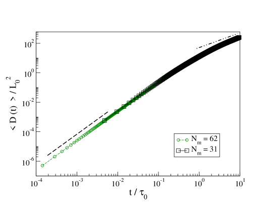
We first consider the absolute dispersion, that is the mean displacement of a single particle with respect to its initial position. The statistical behaviour is expected to be ballistic for correlated scales, followed by simple diffusion á la Taylor at scales larger than the velocity integral scale $L_{0}$. To this aim we compute:

$$D(t)=\langle\left[{\bf x}(t)-{\bf x}(0)\right]^{2}\rangle,$$ (12)

where ${\bf x}(t)$ is the position at time $t$ of a particle that was in ${\bf x}(0)$ at the initial time $t=0$ and the brackets $\langle\cdot\rangle$ indicate ensemble average. From Figure 3, we observe that single particle diffusion is well represented by the model. At time scales of the inertial range, the slope is well approximated by the ballistic $t^{2}$ power law, whereas at large times, $t>\tau_{0}$, the diffusive scaling law sets in.

$N_{m}$	$q_{0}$	$L_{0}$	$l_{N_{m}-1}$	$\tau_{0}$	$\tau_{N_{m}-1}$
$31$	$0.4$	$10$	$5.5\cdot 10^{-2}$	$21$	$6.7\cdot 10^{-1}$
$62$	$0.4$	$10$	$2.6\cdot 10^{-4}$	$21$	$1.9\cdot 10^{-2}$

Table 1: Model parameters, the symbols indicate: $q_{0}$ entering the definition of the rms velocity $u_{0}$; $N_{m}$ the total number of modes; $L_{0}$ and $l_{N_{m}-1}$ the largest and smallest model length scales; $\tau_{0}$ and $\tau_{N_{m}-1}$ the lrgest and the smallest time scales. The ratio of the simulation time step $dt$ to the fastest time scale $\tau_{N_{m}-1}$ is $dt/\tau_{N_{m}-1}\simeq 60$, in both cases.

III.1 Tracer pair dispersion

Figure 4: Log-log plot of the Finite Size Lyapunov Exponent $\lambda(r)$ for the numerical simulations with $N_{m}=31$ (black squares) and $N_{m}=62$ (green circles). The straight dashed lines indicate the $r^{-2/3}$ scaling regime.

The separation statistics of pairs of particles, labeled $1$ and $2$, is defined via the moments of the separation vector ${\bf r}(t)={\bf x}_{1}(t)-{\bf x}_{2}(t)$. In statistically homogeneous and isotropic turbulence, the separation distance $r=|{\bf r}|$ is the key observable for the problem of relative dispersion.
We first report results on the statistics of

$$\langle\left[{\bf r}(t)-{\bf r}_{0}\right]^{2}\rangle_{r_{0}}=\langle\left\{[{\bf x}_{1}(t)-{\bf x}_{2}(t)]-[{\bf x}_{1}(0)-{\bf x}_{2}(0)]\right\}^{2}\rangle\,,$$ (13)

to better highlight the scaling behaviours. Two regimes characterise the pair dispersion for inertial-range initial distances $r_{0}$,

$$\langle\left[{\bf r}(t)-{\bf r}_{0}\right]^{2}\rangle_{r_{0}}\simeq t^{2}S_{2}(r_{0})\,,$$ (14)

$$\langle{\bf r}(t)^{2}\rangle\simeq g\,t^{3}\,.$$ (15)

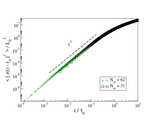
The first behaviour is the so-called Batchelor regime Sawfordrev due to the memory of the initial velocity difference. In eqn. (15), $S_{2}(r)$ is the Eulerian second-order structure function at scale $r$. The Batchelor scaling occurs on time scales of the order of the eddy-correlation time at scale $r_{0}$. The second is the Richardson regime, indipendent of the initial separation, taking place asymptotically on times scales much larger than the eddy-turnover time at scale $r_{0}$, and much smaller than the integral time scale. In Figure 5, we plot $\langle\left[{\bf r}(t)-{\bf r}_{0}\right]^{2}\rangle$, where the average is taken over pairs whose initial separation $r_{0}$ is much smaller that the smallest scale $l_{N_{m}-1}$, accordingly the ballistic regime is very short, and the asymptotic Richardson regime is readily observed.

Figure 5: Log-log plot of particle relative dispersion for the simulations with $N_{m}=31$ (black squares) and $N_{m}=62$ (green circles). The straight line indicates the Richardson $t^{3}$ scaling regime for the inertial range of scales.

The existence of Richardson regime in $3D$ turbulence is often debated. In addition to the memory of the initial conditions, both experimental and numerical measurements have to deal with the limited extension of the inertial range, and with crossover regimes towards the infra-red cut off (from inertial to large scales) and the ultra-violet cutoff (from inertial to dissipative scales).
A better suited observable, allowing to partially overcome issues due to a limited inertial range, is obtained by using fixed-scale statistics artale. It consists of fixing a set of thresholds, $r_{n}=􏲵\rho^{n}r_{0}$, with the factor $\rho>1$ and $n=1,2,3,...$, and then calculating the time $T$ it takes for the pair separation to change from $r_{n}$ to $r_{n+1}$. If $\rho=1$ such time is also called the doubling time. Here we compute the Finite-Size Lyapunov Exponent (FSLE) (Cencinirev ), in terms of the mean time $\langle T_{\rho}(r)\rangle$ it takes for pair separation $r$ to grow to $\rho r$. In the present analysis, we used $\rho=1.25$: note that the choice of $\rho>1$ is irrelevant for the scaling properties, but only fixes the threshold spacing and enters in the mean time expression as a prefactor boff2d ; Pof2005 . The FSLE is defined as:

$$\lambda(r_{n})=\frac{\log\rho}{\langle T_{\rho}(r_{n})\rangle}\,.$$ (16)

In the limit of an infinitesimal threshold $r_{n}$, the FSLE recovers the maximal Lypanuov exponent of the turbulent flow Cencinirev . In our model however there is no tangent space dynamics, and so the FSLE has a well defined meaning only in the inertial range of scales. By dimensional scaling arguments, if the mean separation grows as $\langle r(t)^{2}\rangle\sim t^{3}$, then the FSLE behaves as $\lambda(r)\sim r^{-2/3}$. At scales larger than the integral scale $L_{0}$, we expect $\lambda(r)\sim r^{-2}$.
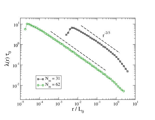
In Fig. 4, we plot the FSLE measurements for the two sets of numerical simulations performed. Since by construction all scales $r$, with $l_{N_{m}-1}<r<L_{0}$, belong to the inertial range, we observe the $\lambda(r)\sim r^{-2/3}$ scaling only. At large scales, we detect a steeper slope, associated to Taylor diffusion, where at small scales, FSLE drops since there is no dissipative range dynamics in this system.

III.2 Tetrad dispersion

The interest in studying the displacement statistics of a bunch of particles is that it can be used to describe moments of a passive scalar field, satisfying an advection-diffusion equation. This has been exploited in the past to assess the intermittent statistics of a passive scalar field advected by a synthetic Gaussian velocity field frismazverg , or by a $2D$ turbulent velocity field in the turbulent regime of inverse cascade of energy celverg . Unfortunately, similar results do not yet exist for $3D$ turbulence. On the other hand, Lagrangian multi-particle motion is very important when studying dispersion and mixing properties, both in ideal (i.e., statistically homogeneous and isotropic) and in real flows.

Figure 6: Log-log plot of the mean eigenvalues of the inertia matrix, as a function of time. The straight line indicates the $t^{3}$ Richardson scaling law for the inertial range of scales.

Beside pair dispersion, tetrad dispersion and its modelling have attracted much attention in the last years pum00 ; Pof2005 ; Dev2013 ; Sawford2013 : indeed, the time evolution of four tracers is the building block of a phenomenological model to describe the Lagrangian dynamics over a volume region with characteristic scales lying in the inertial range CPS99 ; additionally it is a better candidate than a tracer pair to describe geometrical properties in a turbulent flow, such as vortex stretching, and vorticity/strain alignment.
Within the proposed model, we have performed series of simulations with tracer particles initially arranged on regular tetrahedron of side $\l_{N_{m}-1}/2$, so to have a narrow distributions for tetrads initial conditions. Moreover, the initial distribution of the tetrad center of mass and orientation is random uniform in the computational domain. To achieve good statistics, we collected $50$ simulations, each containing $100$ tetrahedron. The model parameters are those listed in Table 1, case $N_{m}=62$.
The evolution of the tetrad shapes in a statistically homogeneous flow is conveniently analyzed by performing a change of coordinate CPS99 , from the particle positions ${\bf x}_{i}$, $i=1,2,3,4$ to the reduced set of coordinates ${\bm{\rho}}_{m}$, $m=0,1,2,3$, defined as:

$${\bm{\rho}}_{0} = \frac{1}{4}\,\sum_{i=1}^{4}{\bf x}_{i}\,,$$ (17)

$${\bm{\rho}}_{m} = \frac{1}{\sqrt{m(m+1)}}\,\sum_{i=1}^{m}({\bf x}_{i}-{\bf x}_{m+1})\,.$$ (18)

While the center of mass diffuses in the flow, the geometrical information is contained in the square symmetric inertia matrix ${\bf I}=\bm{\rho}\bm{\rho}^{T}$, with column vectors $\bm{\rho}_{m}$, $m=1,2,3$. Owing to the homogeneity of the velocity field and of the initial tetrad distribution, the statistics does not depend on the centre of mass ${\bm{\rho}}_{0}$.
The matrix admits real positive eigenvalues, $g_{i}$, that can be ordered according to: $g_{1}\geq g_{2}\geq g_{3}$. The tetrahedron dimension is given by $r=\sqrt{2/3\,tr({\bf I})}=\sqrt{2/3(g_{1}+g_{2}+g_{3})}$ and the volume is $V=1/3\sqrt{det({\bf I})}=1/3\sqrt{g_{1}g_{2}g_{3}}$. It is convenient to introduce the adimensional quantities $I_{i}=g_{i}/r^{2}$ (where $I_{1}+I_{2}+I_{3}=1$), whose relative values give an indication of the tetrahedron shape. For a regular tetrahedron $I_{1}=I_{2}=I_{3}=1/3$; when the four points are coplanar $I_{3}=0$; when they are aligned $I_{2}=I_{3}=0$.
We remark that by means of a stochastic model for tetrad dispersion, Devenish Dev2013 recently obtained values for the $I_{i}$ indices in agreement with those of Direct Numerical Simulations of $3D$ turbulence.
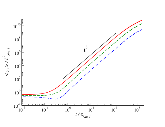
In Fig. 6 we present the temporal evolution of the mean eigenvalues of ${\bf I}$. Numerical results show good agreement with Richardson prediction, i.e. $\langle g_{i}\rangle\simeq t^{3}$. This issue is further verified by measuring fixed scale statistics. To this aim we compute the average time $\langle T_{\alpha}(g_{i})\rangle$ it takes for each eigenvalue $g_{i}$ to increase its value of a factor $\alpha$, with $\alpha=2$, i.e. $\langle T_{\alpha}(g_{i})\rangle$ are the average eigenvalues doubling times.
Results are plotted in Fig. 7. They indicate the existence of a wide inertial range, where the slope of the exit-time is $g_{i}^{1/3}$, matching Richardson prediction. In addition, in the inset, the three eigenvalues overlap after rescaling $g_{1}$ and $g_{2}$ respectively with the factors $100$ and $15$. These scaling factors yield to $I_{1}\simeq 0.862$, $I_{2}\simeq 0.129$, $I_{3}\simeq 0.0086$, i.e. very elongated tetrahedron.

Figure 7: Mean exit-time values for the eigenvalues of the inertia matrix. In the inset the three curves, after rescaling $g_{1}$ and $g_{2}$ with the factors $100$ and $15$, respectively, to obtain an overlap.

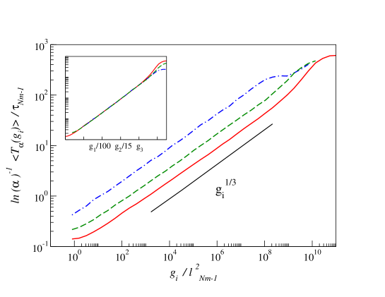
The existence of a range where, after rescaling on the horizontal axis, the values of the exit-time are the same for the three eigenvalues implies that the tetrads increase their dimension while maintaining the same (elongated) shape. The results can be compared with the DNS of Pof2005multi . They show qualitative agreement, though the values of the rescaling factors applied to achieve the exit-times collapse are different.
In Fig. 8 (left) we present the behaviour of the $\langle I_{i}\rangle$, with $i=1,2,3$ as a function of time. The coefficients present, over a large time interval, values consistent with elongated tetrahedron; then, for $t/\tau_{0}\sim 1$ (i.e. $t/\tau_{N_{m}-1}\sim O(10^{3})$) they tend to the values obtained for tetrads formed from Gaussian distributed particles pum00 .

Figure 8: Average shape parameters $\langle I_{i}\rangle$ as a function of time. On the left: average upon all tetrads. The straight lines indicate the asymptotic values for Gaussian distributed particles $I_{1}=0.75$, $I_{2}=0.22$, $I_{3}=0.03$. On the right: average upon tetrads whose $g_{i}$ belongs to the inertial range. The straight lines are best fits for $1<t/\tau_{Nm-1}<100$: $I_{1}=0.833$, $I_{2}=0.151$, $I_{3}=0.0155$.

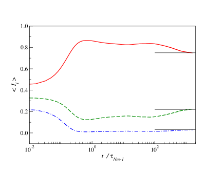
In Fig. 8 (right) the $\langle I_{i}\rangle$ are computed selecting at each time step those $g_{i}$, for which the exit-time follows Richardson scaling law, i.e. $1<g_{1}/l_{Nm-1},\,g_{2}/l_{Nm-1}<10^{9}$, $1<g_{3}/l_{Nm-1}<10^{8}$. The figure shows the presence of a plateau where the values of the indexes are $\langle I_{1}\rangle=0.833\pm 0.004$, $\langle I_{2}\rangle=0.151\pm 0.003$, and $\langle I_{3}\rangle=0.0155\pm 0.0007$. Again, there is some discrepancy with the direct numerical simulations results for HIT, where it was measured $\langle I_{3}\rangle=0.011\pm 0.001$ and $\langle I_{2}\rangle=0.135\pm 0.003$ Pof2005 . However these values confirm the presence of elongated structures in the inertial range, with the index $\langle I_{3}\rangle$ larger with respect to the expectation value for Gaussian distributed particles.

IV Conclusion

A novel Lagrangian model is presented aimed at accurately reproducing the statistical behaviour of clouds of particles dispersed in statistically isotropic and homogeneous, incompressible turbulent flows. The model reflects the multi-scale nature of the direct energy cascade of $3D$ turbulence. While the model is primarily meant to be used as a sub-grid model -it evolves fluid tracers sub-grid velocities that are correlated according to their relative distances-, it may be adapted to solve the Navier-Stokes equations by a Lagrangian approach (in the spirit of smoothed-particle hydrodynamics solvers).
To assess the model performances and accuracy, we presented several validations based on comparison with recent investigation on the phenomenology of fluid tracers in high-resolution, high-statistics Direct Numerical Simulations. The first validation consisted in performing two simulations that differ only by total number of modes, while the large length and velocity scales are kept constant. We showed that the model can reproduce Richarson law for the pair dispersion statistics. It is important to stress that the width of the inertial range can be apriori fixed by tuning the sub-grid model parameters. With respect to multi-particle statistics, we analysed the dispersion of tracers initially located on the side points of tetrahedra. Also in this case we could detect a good agreement with results obtained in direct numerical simulations of homogeneous and isotropic turbulence Pof2005multi .
Two important approximations have been adopted to build up the model: statistics is Gaussian and self-similar. Deviations from Gaussianity could be of interest if the tracer particle model is used to reproduce stationary statistics of turbulent velocity increments (e.g. the four-fifth law) Pagnini . In the present formulation of the model, we neglected such feature and showed that this does not affect results for pair and tetrad dispersion.
Neglecting intermittency may also be a limitation since non self-similar corrections to the Richardson’s picture have been detected in the tails of pair separation distribution BoffSok3D ; SBTPRL2012 . Intermittency could be introduced by building up synthetic multiaffine processes BBCCV98 ; toschi_bode . This is left for future investigations.
Based on the accuracy of the results, it appears that the potential of the model for practical use is high. First of all, it can be applied, within the restrictions discussed in the paper, to an arbitrary number of fluid tracers and the computational cost will grow with the number of tracers. Moreover the model parameters can be choosen to achieve the desired extension of the inertial range. Finally, the absence of a grid makes the method suitable also for complex situations, for instance in the presence of free surfaces. The capabilities of the model in more complex flows, e.g. shear and channel flows, will be a matter of future investigations. Finally, the model may be easily modified to describe inertial heavy point-like particles MaxeyRiley1983 .

*

Appendix A Particle Spatial Distribution

In order to test particle model incompressibility, we performed the following experiment. We seeded a periodic cubic domain with ${\cal N}=1000$ particles, uniformly distributed and with $N_{m}=31$ velocity modes, that we followed for a few large eddy-turnover times, $\tau_{0}$. An uniform distribution of ${\cal N}$ particles in the volume ${\cal V}$ means that, after coarse-graining the volume in cells of size $R$, the number of particles in each cell, dubbed $n$, will be a random variable with Poisson distribution,

$$p_{R}(n)=\frac{(\lambda_{R})^{n}}{n!}\exp{(-\lambda_{R})}\,.$$ (19)

Here $\lambda_{R}={\cal N}/(L/R)^{3}$ is the average number of particles in a cell of size $R^{3}$ and ${\cal V}=L^{3}$ is the total volume considered. From (19), it is easy to derive:

$$\langle n^{2}\rangle=\langle n\rangle^{2}+\langle n\rangle.$$ (20)

Possible deviations from the uniform distribution can be systematically quantified, scale by scale, in terms of the coefficient:

$$\mu(R)=\frac{\sigma_{R}^{2}}{\lambda_{R}^{2}}=\frac{\langle n^{2}\rangle-\langle n\rangle^{2}}{\langle n\rangle^{2}},$$ (21)

where for a uniform distribution $\langle n\rangle=\lambda_{R}=\rho R^{3}$ where $\rho={\cal N}/{\cal V}$ is the particle number density, and thus $\mu(R)=1/(\rho R^{3})$. Deviation from such behaviour can be also quantified in terms of the two-points correlation in the particle distribution.
The test has been performed within three periodic boxes of sides, respectively, $2L_{0}$, $4L_{0}$ and $8L_{0}$, results are presented in Figure 9. The plots show that, on the small scales, uniformity is retained during the temporal evolution. However, on the large scales, spatial correlations may develop, being more intense when the box dimension is of the same order of the large eddy scale, and decaying at increasing the ratio $L/L_{0}$. Therefore, for $L/L_{0}\gg 1$, particle spread uniformly within the domain, at all scales.

Note that, in order to take into account of molecular diffusion on the smallest scales (i.e. scales smaller than $l_{N_{m}-1}$) a random fluctuation could be added to the velocity of coincident particles. In fact, according to our model, two or more particles, residing at the same location at the same time, will be subjected to the same velocity, so they will stick together for all subsequent times, while molecular diffusion would guarantee that coincident particles always separate, see Tho90 . In practice we found that it was not needed to include this random diffusion because these occurance are very unlikely, as it is also indicated by the behaviour of $\mu(R)$ on the very small scales.

Figure 9: Coefficient $\mu(R)$ as a function of $R/L$ for simulation with $L=2L_{0}$ (left); $L=4L_{0}$ (centre) and $L=8L_{0}$ (right). Results indicate: time $t=0$ (black pluses), time $t=2\tau_{0}$ (red crosses) and the uniform distribution expectation, $1/(\rho R^{3})$ (black straight line).

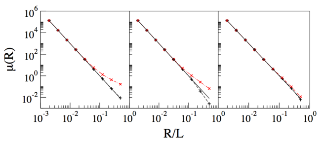
Results of Fig. 9 have a clear interpretation: particles tend to spread uniformly, but the velocity modulation on the large scales induces a spatial correlations. These can be further quantified and controlled according to the simple arguments that follows.
Starting from any initial spatial condition, when $t>\tau_{0}$ the average distance of one particle to its closest neighbour, $d_{1}$, can be estimated by the expression cha43 :

$$d_{1}=\frac{1}{\pi^{1/2}}\Big{[}\Gamma\Big{(}\frac{D}{2}+1\Big{)}\Big{]}^{1/D}\Gamma\Big{(}1+\frac{1}{D}\Big{)}\Big{(}\frac{{\cal V}}{{\cal N}}\Big{)}^{1/D}\,,$$ (22)

where $\Gamma$ is the Euler Gamma function, $D=3$ the space dimension, ${\cal V}$ the volume and ${\cal N}$ the total number of particles. Numerical results agree with the theoretical expectation for randomly distributed particles, eq. (22). The deviation of $\mu(R)$ from $1/(\rho R^{3})$ occurs at a scale $R\sim d_{1}$ (i.e. $R/L\sim 0.055$ for ${\cal N}=1000$), because mode velocities on all scales larger than $d_{1}$ are correlated. Clearly, the larger the number of correlated modes, the stronger the deviations from uniformity.

Figure 10: Average $n$-th neighbour distance for $n<100$. The curves represent: the theoretical expectation with error bars (cyan), simulation with $L/L_{0}$ respectively equal to $8$ (black pluses) $4$ (green crosses) and $2$ (red circles).

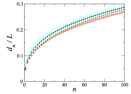
We remark that, when $L_{0}=10$ and $N_{m}=31$, there are $13$ modes with length scale larger than $d_{1}=1.1$ (average particle distance in simulations with $L=2L_{0}$) and only $5$ modes with length scale larger than $d_{1}=4.4$ (average distance when $L=8L_{0}$). This explains the more intense deviations detected in the left plot of Figure 9 with respect to the right plot.
In general, the number of correlated modes $N_{c}$ depends on the integral scale $L_{0}$, on the model parameter $\lambda$, and on the particle density $\rho$, according to:

$$N_{c} = int\left(1+log_{\lambda}\frac{L_{0}}{d_{1}}\right)$$ (23)

$$= int\left(1+log_{\lambda}\left(\frac{\sqrt{\pi}\,L_{0}\,\rho^{1/3}}{\Gamma(5/2)^{1/3}\,\Gamma(4/3)}\right)\right).$$ (24)

The average distance $d_{n}$ of a particle to its $n$-th neighbour can also be computed. Recalling that one point is the $n$-th neighbor of another one if there are exactly $n-1$ other points that are closer to the latter than the former, the distance $d_{n}$, in the case of ${\cal N}$ uniformly distributed particles, is per96 :

$$\frac{d_{n}}{L}=$$ (25)

$$\frac{1}{\pi^{1/2}}\Big{[}\Gamma(\frac{D}{2}+1)\Big{]}^{1/D}\frac{\Gamma(n+\frac{1}{D})}{\Gamma(n)}\Big{(}\frac{1}{{\cal N}}\Big{)}^{1/D}\,,$$

with the mean square fluctuation ,

$$\left(\frac{\Delta d_{n}}{L}\right)^{2}=$$ (26)

$$\frac{1}{\pi}\left[\Gamma(\frac{D}{2}+1)\right]^{2/D}\left[\frac{\Gamma(n+\frac{2}{D})}{\Gamma(n)}-\frac{\Gamma^{2}(n+\frac{1}{D})}{\Gamma^{2}(n)}\right]\left(\frac{1}{{\cal N}}\right)^{2/D}.$$

Results for the three test cases are presented in Figure 10, as a function of the neighbour index $n$. They show that, when ${\cal N}=1000$, only the simulation with $L/L_{0}=8$ has average $n$-th neighbour distance consistent, within error bars, with the theoretical prediction (eqs. (A) - (A)). Thus, we infer that the ratio of correlated modes, $N_{c}$, to the total number of modes, $N_{m}$, has to be rather small in order for the model to satisfy incompressibility. The present indication is that $N_{c}/N_{m}\simeq 1/6$ is enough to produce uniformity at all scales (see Figure 9). When the present model is employed as a subgrid-scale Lagrangian model this restriction should not apply as the evolution on the larger scales will be matched with the resolved modes of the LES.

References

- (1) H. J. S. Fernando and D. Zajic and S. Di Sabatino and R. Dimitrova and B. Hedquist and A. Dallman, “Flow, turbulence and pollutant dispersion in urban atmospheres,” Phys. Fluids 22, 051301 (2010).
- (2) R. Scatamacchia and L. Biferale and F. Toschi, “Extreme Events in the Dispersions of Two Neighboring Particles Under the Influence of Fluid Turbulence,” Phys. Rev. Lett. 109, 144501 (2012).
- (3) F. Toschi and E. Bodenschatz, “Lagrangian Properties of Particles in Turbulence,” Ann. Rev. Fluid Mech. 41, 375 (2009).
- (4) N.S. Holmes and L. Morawska, “Review of Dispersion Modelling and its application to the dispersion of particles: An overview of different dispersion models available,” Atmos. Environ. 40, 5902 (2006).
- (5) M. Chamecki and C. Meneveau, “Particle boundary layer above and downstream of an area source: scaling, simulations, and pollen transport,” J. Fluid Mech. 683, 26 (2011).
- (6) G. Lacorata and A. Mazzino and U. Rizza, “3D Chaotic Model for Subgrid Turbulent Dispersion in Large Eddy Simulations,” J. Atmos. Sci. 65:7, 2389 (2008).
- (7) A. S. Lanotte and I. M. Mazzitelli, “Scalar Turbulence in Convective Boundary Layers by Changing the Entrainment Flux,” J. Atmos. Sci. 70, 248 (2013).
- (8) S. Berti and F. A. Dos Santos and G. Lacorata and A. Vulpiani, “Lagrangian Drifter Dispersion in the Southwestern Atlantic Ocean,” J. Phys. Ocean. 41, 1659 (2011).
- (9) L. Palatella and F. Bignami and F. Falcini and G. Lacorata and A. S. Lanotte and R. Santoleri, “Lagrangian simulations and inter-annual variability of anchovy egg and larva dispersal in the in the Sicily Channel,” accepted on J. Geophys. Res. - Ocea. (2014).
- (10) R. A. Shaw, “Particle-turbulence interactions in atmospheric clouds,” Ann. Rev. Fluid Mech. 35, 183 (2003).
- (11) M. U. Baëbler and M. Morbidelli and J. Bałdyga, “Modelling the breakup of solid aggregates in turbulent flows,” J. Fluid Mech. 612, 261 (2008).
- (12) M. U. Baëbler and L. Biferale and A. S. Lanotte, “Breakup of small aggregates driven by turbulent hydrodynamical stress,” Phys. Rev. E 85, 025301(R) (2012).
- (13) S. Post and J. Abraham, “Modeling the outcome of drop-drop collisions in Diesel sprays,” Int. J. of Multiphase Flow 28, 997 (2002).
- (14) P. Segaut, Large Eddy Simulation for Incompressible Flows (Third ed.), Springer (2006).
- (15) C. Meneveau and J. Katz, “Scale-Invariance and Turbulence Models for Large-Eddy Simulation,” Annu. Rev. Fluid Mech. 32(1), 1 (2000).
- (16) P.P. Sullivan and J. C. McWilliams and C.-H. Moeng, “A sub-grid-scale model for large-eddy simulation of planetary boundary layer flows.” Bound.-Layer Meteor. 71, 247 (1994).
- (17) E. Lévêque and F. Toschi and L. Shao and J.-P. Bertoglio, “Shear-improved Smagorinsky model for large-eddy simulation of wall-bounded turbulent flows,” J. Fluid Mech. 570, 491 (2007).
- (18) S. Ott and J. Mann, “An experimental investigation of the relative diffusion of particle pairs in three-dimensional turbulent flows,” J. Fluid Mech. 422, 207 (2000).
- (19) A. La Porta and G. A. Voth and A. M. Crawford and J. Alexander and E. Bodenschatz, “Fluid particle accelerations in fully developed turbulence,” Nature 409, 1017 (2001).
- (20) N. Mordant and P. Metz and O. Michel and J. F. Pinton, “Measurement of Lagrangian velocity in fully developed turbulence,” Phys. Rev. Lett. 87, 214501 (2001).
- (21) T. Ishihara and Y. Kaneda, “Relative diffusion of a pair of fluid particles in the inertial subrange of turbulence,” Phys. Fluids 14(11), L69 (2002).
- (22) P. K. Yeung and M.S. Borgas, “Relative dispersion in isotropic turbulence: part 1. Direct numerical simulations and Reynolds number dependence,” J. Fluid Mech. 503, 125 (2004).
- (23) G. Boffetta and I. M. Sokolov, “Relative dispersion in fully developed turbulence: The Richardson’s law and intermittency corrections,” Phys. Rev. Lett. 88, 094501 (2002).
- (24) L. Biferale and G. Boffetta and A. Celani and B.J. Devenish and A. Lanotte and F. Toschi, “Multifractal statistics of Lagrangian velocity and acceleration in turbulence,” Phys. Rev. Lett. 93, 064502 (2004).
- (25) L. Biferale and G. Boffetta and A. Celani and B.J. Devenish and A. Lanotte and F. Toschi, “Lagrangian statistics of particle pairs in homogeneous isotropic turbulence,” Phys. Fluids 17, 115101 (2005).
- (26) P.K. Yeung, “Lagrangian investigations of turbulence,” Annu. Rev. Fluid Mech. 34, 115 (2002).
- (27) B. Sawford, “Turbulent relative dispersion,” Annu. Rev. Fluid Mech. 33, 289 (2001).
- (28) J.P.L.C. Salazar and L.R. Collins, “Two-Particle Dispersion in Isotropic Turbulent Flows,” Annu. Rev. Fluid Mech. 41, 435 (2009).
- (29) J. Bec and L. Biferale and A.S. Lanotte and A. Scagliarini and F. Toschi, “Turbulent pair dispersion of inertial particles,” J. Fluid Mech. 645, 1 (2010).
- (30) J. C. Weil and P.P. Sullivan and C.-H. Moeng, “The Use of Large-Eddy Simulations in Lagrangian Particle Dispersion Models,” J. Atmos. Sci. 61, 2877 (2004).
- (31) G. Jin and G.-W. He, “A nonlinear model for the subgrid timescale experienced by heavy particles in large eddy simulation of isotropic turbulence with a stochastic differential equation,” New J. Phys. 15, 035011 (2013).
- (32) G. Falkovich and K. Gawȩdzki and M. Vergassola, “Particles and fields in fluid turbulence,” Rev. Mod. Phys. 73, 913 (2001).
- (33) M. Chertkov and A. Pumir and B. Shraiman, “Lagrangian tetrad dynamics and the phenomenology of turbulence,” Phys. Fluids 11, 2394 (1999).
- (34) L. Biferale and G. Boffetta and A. Celani and B.J. Devenish and A. Lanotte and F. Toschi, “Multiparticle dispersion in fully developed turbulence,” Phys. Fluids 17, 111701 (2005).
- (35) H. Xu and N. T. Ouellette and E. Bodenschatz, “Evolution of geometric structures in intense turbulence,” New J. Phys. 10, 013012 (2008).
- (36) J. F. Hackl and P.K. Yeung and B.L. Sawford, “Multi-particle and tetrad statistics in numerical simulations of turbulent relative dispersion,” Phys. Fluids 23, 065103 (2011).
- (37) A. Arnéodo et al., “Universal Intermittent Properties of Particle Trajectories in Highly Turbulent Flows,” Phys. Rev. Lett. 100, 254504 (2008).
- (38) D. J. Thomson, “Criteria for the selection of stochastic models of particle trajectories in turbulent flows,” J. Fluid Mech. 180, 529 (1987).
- (39) H. Kaplan and N. Dinar, “A three dimensional stochastic model for concentration fluctuation statistics in isotropic homogeneous turbulence,” J. Comput. Phys. 79, 317 (1998).
- (40) D. J. Thomson, “A stochastic model for the motion of particle pairs in isotropic high-Reynolds number turbulence, and its application to the problem of concentration variance,” J. Fluid Mech. 210, 113 (1990).
- (41) O. A. Kurbanmuradov, “Stochastic Lagrangian models for two-particle relative dispersion in high-Reynolds number turbulence,” Monte Carlo Meth. Appl. 3, 37 (1997).
- (42) B. J. Devenish and D. J. Thomson, “A Lagrangian stochastic model for tetrad dispersion”, Journ. Turb. 14,3 (2013).
- (43) B. J. Devenish, “Geometrical Properties of Turbulent Dispersion,” Phys. Rev. Lett. 110, 064504 (2013).
- (44) J. C. H. Fung and J. C. R. Hunt and N. A. Malik and R. J. Perkins, “Kinematic simulation of homogeneous turbulent flows generated by unsteady random Fourier modes,” J. Fluid Mech. 236, 281 (1992).
- (45) J. C. H. Fung and J. C. Vassilicos, “Two-particle dispersion in turbulentlike flows,” Phys. Rev. E 57, 1677 (1998).
- (46) M. Chaves and K. Gawȩdzki and P. Horvai and A. Kupiainen and M. Vergassola, “Lagrangian dispersion in Gaussian self-similar velocity ensembles,” J. Stat. Phys. 133, 643 (2004).
- (47) D. J. Thomson and B. J. Devenish, “Particle pair separation in kinematic simulations,” J. Fluid Mech. 526, 277 (2005).
- (48) G. L. Eyink and D. Benveniste, “Suppression of particle dispersion by sweeping effects in synthetic turbulence,” Phys. Rev. E 87(2), 023011 (2013).
- (49) J. G. M. Kuerten, “Subgrid modeling in particle-laden channel flow,” Phys. Fluids 18, 025108 (2006).
- (50) C. Marchioli and M.V. Salvetti and A. Soldati, “Some issues concerning Large-Eddy Simulation of inertial particle dispersion in turbulent bounded flows,” Phys. Fluids 20, 040603 (2008).
- (51) E. Calzavarini and A. Donini and V. Lavezzo and C. Marchioli and E. Pitton and A. Soldati and F. Toschi, “On the Error Estimate in Sub-Grid Models for Particles in Turbulent Flows,” in Direct and Large-Eddy Simulation VIII. ERCOFTAC Series, Springer Netherlands, 15, 171–176 (2011).
- (52) J. J. Monaghan, “Smoothed Particle Hydrodynamics and Its Diverse Applications,” Annu. Rev. Fluid Mech. 44, 323 (2012).
- (53) B. L. Sawford and S. B. Pope and P. K. Yeung, “Gaussian Lagrangian stochastic models for multi-particle dispersion,” Phys. Fluids 25, 055101 (2013).
- (54) M. S. Borgas and B. L. Sawford, “A family of stochastic models for two-particle dispersion in isotropic homogeneous stationary turbulence,” J. Fluid Mech. 279, 69 (1994).
- (55) T. Burgener and D. Kadau and H. Herrmann, “Particle and particle pair dispersion in turbulence modeled with spatially and temporally correlated stochastic processes,” Phys. Rev. E 86, 046308 (2012).
- (56) U. Frisch, Turbulence. The legacy of A. N. Kolmogorov, Cambridge University Press, New York (1995).
- (57) D. T. Gillespie, “Exact numerical simulation of the Ornstein-Uhlenbeck process and its integral,” Phys. Rev. E 54, 2084 (1996).
- (58) S. B. Pope, Turbulent Flows, Cambridge University Press (2000).
- (59) C. Meneveau, “Transition between viscous and inertial-range scaling of turbulence structure functions,” Phys. Rev. E 54, 3657 (1996).
- (60) V. Artale and G. Boffetta and A. Celani and M. Cencini and A. Vulpiani, “Dispersion of passive tracers in closed basins: Beyond the diffusion coefficient,” Phys. Fluids 9, 3162 (1997).
- (61) M. Cencini and A. Vulpiani, “Finite Size Lyapunov Exponent: review on applications,” J. Phys. A: Math. Theor. 46, 254019 (2013).
- (62) G. Boffetta and I. M. Sokolov, “Statistics of two-particle dispersion in two-dimensional turbulence,” Phys. Fluids 14, 3224 (2002).
- (63) U. Frisch and A. Mazzino and M. Vergassola, “Intermittency in Passive Scalar Advection,” Phys. Rev. Lett. 80, 5532 (1998).
- (64) A. Celani and M. Vergassola, “Statistical geometry in scalar turbulence,” Phys. Rev. Lett.q 86(3), 424 (2001).
- (65) A. Pumir and B. I. Shraiman and M. Chertkov, “Geometry of Lagrangian dispersion in turbulence,” Phys. Rev. Lett. 85, 5324 (2000).
- (66) G. Pagnini, “Lagrangian stochastic models for turbulent relative dispersion based on particle pair rotation,” J. Fluid Mech. 616, 357 (2008).
- (67) L. Biferale and G. Boffetta and A. Celani and A. Crisanti and A. Vulpiani, “Mimicking a turbulent signal: Sequential multiaffine processes,” Phys. Rev. E 57(6), R6261 (1998).
- (68) M. R. Maxey and J. Riley, “Equation of motion of a small rigid sphere in a nonuniform flow,” Phys. Fluids 26, 883 (1983).
- (69) S. Chandrasekar, Rev. Mod. Phys. 15, 1 (1943).
- (70) A. G. Percus and O. C. Martin, “Finite Size and Dimensional Dependence in the Euclidean Traveling Salesman Problem,” Phys. Rev. Lett. 76, 1188 (1996).