33email: monari@astro.rug.nl
The Galactic bar and the large scale velocity gradients in the Galactic disk
Abstract
Aims. We investigate whether the cylindrical (galactocentric) radial velocity gradient of , directed radially from the Galactic center and recently observed in the stars of the solar neighborhood with the RAVE survey, can be explained by the resonant effects of the bar near the solar neighborhood.
Methods. We compared the results of test particle simulations of the Milky Way with a potential that includes a rotating bar with observations from the RAVE survey. To this end we applied the RAVE selection function to the simulations and convolved these with the characteristic RAVE errors. We explored different “solar neighborhoods” in the simulations, as well as different bar models.
Results. We find that the bar induces a negative radial velocity gradient at every height from the Galactic plane, outside the outer Lindblad resonance and for angles from the long axis of the bar compatible with the current estimates. The selection function and errors do not wash away the gradient, but often make it steeper, especially near the Galactic plane, because this is where the RAVE survey is less radially extended. No gradient in the vertical velocity is present in our simulations, from which we may conclude that this cannot be induced by the bar.
Key Words.:
Galaxy: kinematics and dynamics – Galaxy: solar neighborhood – Galaxy: structure – Galaxy: evolution1 Introduction
Many of the past efforts in modeling the mass distribution of the Milky Way have assumed that the Galaxy is axisymmetric and in a steady state. However, there is a wealth of evidence that these assumptions are not really valid. The two most important deviations from axisymmetry are the spiral arms and the bar. These features are not only apparent as non-axisymmetric density enhancements, but they also have long-range gravitational effects. In particular, the bar modifies the kinematics of the outer parts of the Galactic disks, far beyond its extension, through resonant interactions.
That the velocity distribution of stars very near to the Sun is not smooth (as one would expect in a steady state axisymmetric system), but instead rich in substructures, has been established observationally thanks to data from the Hipparcos satellite and other surveys (Dehnen 1998; Famaey et al. 2005; Antoja et al. 2008). Several authors have explained these substructures as being due to orbital resonant effects of the bar (Dehnen 2000; Fux 2001), of the spiral arms (Mayor 1970; De Simone et al. 2004; Antoja et al. 2011), or both (Antoja et al. 2009; Quillen et al. 2011).
Using data from the RAVE survey (Steinmetz et al. 2006), Antoja et al. (2012) discovered that some of the kinematic substructures detected in the vicinity of the Sun can be traced further, both on and above the plane of the Galaxy, up to .
But RAVE also made it possible to discover large scale streaming motions. Siebert et al. (2011a) (in the rest of the paper S11) used a sample of stars to discover a gradient in the mean galactocentric radial velocity that decreases outward with Galactic radius. S11 show that this gradient was also present when using only the red clump stars in their sample, whose distances are more accurate. Siebert et al. (2012) modeled the gradient as caused by a long-lived spiral pattern. Williams et al. (2013) (hereafter W13) studied the 3D velocity distribution of red clump stars in RAVE in detail, confirmed the existence of the radial velocity gradient and also discovered a more complicated vertical velocity distribution than expected, attributing it to secular phenomena in the Galaxy. Faure et al. (2014) generalized to 3D the model for the spiral arms presented in Siebert et al. (2012), which now also depends on the distance from the Galactic plane. This model nicely predicts a behavior for the mean vertical velocity that is similar to what is observed in W13 (i.e., resembling “rarefaction-compression” waves), together with the radial velocity gradient.
On the other hand, Monari et al. (2013) (hereafter M13), used 3D test particle simulations to show that the gravitational effects of the bar can significantly affect the kinematics of stars near the Sun, even at distances from the Galactic plane up to at least for the thin disk and for the thick disk. These results imply that some of the substructures found in Antoja et al. (2012) could also be caused by the bar.
In this paper we investigate an alternative explanation for the observed radial velocity gradient, beyond that caused by the spiral arms, by suggesting that it can be created by the bar. To do so, we compare the results of the test particle simulations in M13 with the RAVE data.
The paper is organized as follows. In Sect. 2 we summarize the salient characteristics of the simulations from M13, and in Sect. 3 we describe how we apply the RAVE selection function and error convolution to them, to mimic a RAVE catalog. In Sect. 4 we present the results. In Sect. 5 we explain how the bar can create a radial velocity gradient as observed. In Sect. 6 we discuss the similarities between our results and the ones in W13 and in Sect. 7 we conclude.
2 Simulations
We use the 3D test particle simulations of the thin and thick disk of the Milky Way described in M13. The rigid background gravitational potential in these simulations includes an axisymmetric part (composed of a dark halo, and a thin and a thick disk) and a non-axisymmetric perturbation to represent the Galactic bar. The bar potential follows a Ferrers (1870) model and we varied its structural parameters (with values taken from the literature) but with a constant pattern speed . For the comparison with the RAVE data we focus on simulations with three bar potentials: the default bar, the long bar, and the less massive bar (corresponding to GB2, LB2, and GB1 in M13). We choose the snapshot of the simulations at , which corresponds to after the introduction of the bar in the simulations (see M13). In the default bar case, there are particles in the thin disk population and particles in the thick disk (to have a thick-to-thin density of particles normalization of at the Sun). For the remaining cases we only have low resolution simulations with and particles for the thin and the thick disk, respectively. The parameters of the simulations are summarized in Table 1.
In this paper are the Galactocentric cylindrical coordinates, where is the angle from the long axis of the bar in the direction of rotation of the Galaxy. The cylindrical velocities are . Right ascension, declination, and heliocentric distance are denoted as , and the proper motions and line of sight velocity as .
| Parameter | Default bar | Long bar | Less massive bar |
|---|---|---|---|
3 Selection function and errors
3.1 Red clump stars
Both S11 and W13 use red clump stars because they are promising standard candles, since they are easy to identify in the HR diagram, and while being relatively unaffected by extinction their -band magnitude depends only weakly on metallicity and age. In W13 the red clump is selected from the internal RAVE release from October 2011111Here is used to denote -band magnitudes in the system, while and denote the and -band magnitudes in the Bessell & Brett (1989) system. (see the DR3 paper, Siebert et al. 2011b, for stellar parameter determination), as those stars with
| (1) |
The absolute magnitude associated with the red clump stars is taken to be , following Alves (2000).
3.2 RAVE selection function
We applied the RAVE selection function in the space of observables to the simulations. We did this as follows:
-
•
we chose the position of the Sun in the simulated Galaxy; the default position is , in the range of current determinations (Bissantz & Gerhard 2002);
-
•
we transformed the spatial coordinates of the simulation into the observables and heliocentric distance ;
-
•
we assigned magnitudes to the particles in the simulation, assuming they are red clump stars with . Then the apparent magnitude is given by ;
-
•
we binned the red clump stars used in W13 in the space, with bins of size and , , ;
-
•
we binned in the same space and in the same way the particles from the simulation that are inside a sphere of radius from the Sun;
-
•
for , if the -th bin in the simulation contains particles (where is the number of stars in the same bin in RAVE ) we randomly downsampled it to particles; if we kept the particles (because and differ less than the corresponding Poisson noise error); however, not all the bins of the simulations are populated enough: we excluded from the comparison those bins with (this only happened for less than of the bins for the high resolution simulations, and also in the low resolution case after the treatment explained in Sect. 4.3).
We repeated this procedure obtaining different random samples of each simulation, where the , and distribution are almost perfectly matched and the total number of star particles differs from the RAVE red clump sample in W13 by less than for the high resolution simulations, leaving particles in the default bar case.
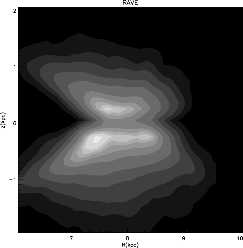

The top panel of Fig. 1 shows the distribution of red clump stars in W13, while in the bottom we have plotted the result of the procedure described above for our standard simulation and Sun’s position. We see that we are successful in reproducing how the different RAVE fields are populated. The differences in (e.g., inside the contour enclosing of the stars) are due to the small differences described above in the bins in the space.
3.3 Error convolution
For the comparison between data and simulations we proceeded to convolve the latter with the errors estimated for the RAVE survey.
We produced a simple error model, where the errors in proper motion and line of sight velocity are function of the magnitude only. This was done by fitting second order polynomials to vs. and vs. for the red clump stars in DR3. We also derived an error in distance propagating the error in () and the spread in absolute magnitudes of the red clump (, Alves 2000). The resulting relative error in distance is , that we assumed to be the same for all particles in our simulations.
The error convolution was done in the observable space , assuming Gaussian errors in each quantity.
4 Results
4.1 Default case
As a default case we place the Sun at and we choose the default bar model. In this case , where is of the Sun and is the Galactocentric distance of the outer Lindblad resonance.
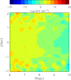
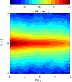
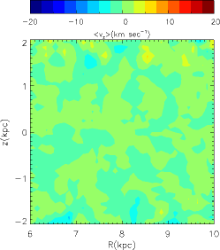
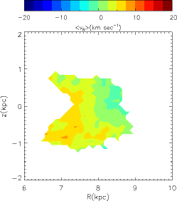
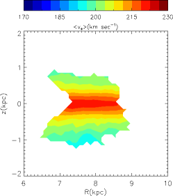
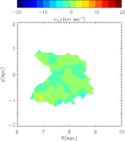
The top row of Fig. 2 shows the average velocities as a function of and , for all the particles inside a sphere of radius from the Sun, with no error convolution yet applied. From left to right we show contour plots of , , and . As in W13, the data are averaged inside bins of size in , box smoothed on a scale of . As it is apparent from these plots, decreases increasing the distance in the simulated Galaxy. Moreover, is rather symmetric with . The central panel shows that the rotational velocity of the stars in the Galactic disk(s) decreases with distance from the plane. This is because the velocity dispersion increases with and because the asymmetric drift increases with the velocity dispersion (Binney & Tremaine 2008). The rightmost panel shows instead how everywhere in the simulated sample, i.e., the distribution function of our simulations is an even function of .
The bottom row of Fig. 2 shows the same quantities as in the top panels, after the application of the RAVE selection function. The plotted values were obtained averaging over the random samples of the simulation, distributed in as in RAVE. We only consider the bins including more than particles. These contour plots show that the decreasing gradient is preserved after the selection function has been applied to the simulation. In fact the gradient is even enhanced: the yellow regions at are formed by particles with , and the blue/green regions at by particles with slightly negative . From the second and third panel we also see that the selection function does not induce any significant difference in and : unlike W13, in the samples presented in this work we do not detect any significant gradient with respect to or .
The reason why the selection function enhances the gradient is readily understood from Fig. 3.
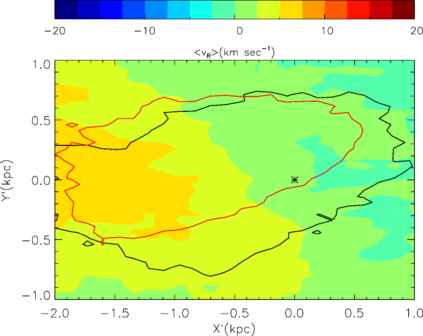
Here and are the cartesian coordinates centered at the Sun, the Galactic Center is placed at , and the colors represent for particles inside a sphere of radius from the Sun in bins of size. The contours enclose of particles with (black) and (red), when the RAVE selection function is applied. These contours therefore show that the selection function encloses mostly particles with negative and positive (with ), where the gradient is steeper.
This analysis shows that is the velocity component most influenced by the bar (and that no signature is readily apparent in ) and therefore we focus in the rest of the paper on the gradients of and on their dependence on .


In Fig. 4 we look closer at the trends with , slicing the particles at different . The quantity is computed inside bins of size . The black line has been obtained using all the particles in the simulations inside a sphere of radius from the Sun, the red line those that remain after applying the RAVE selection function only, and the blue line the case where the error convolution is applied together with the selection function. The shaded areas represent the standard errors of the mean inside each bin. For the red and blue curves we show the maximum error amongst the random samples222We could not use the standard deviation of these 100 random samples, as they are not completely independent. This is because in some of the bins there are as many particles in the simulations as stars in the RAVE red clump sample.. We only show the bins with errors smaller than and including more than particles. The black line confirms what we saw in Fig. 2, namely that decreases with in each of the slices in .
The numbers in the bottom right of each panel quantify the magnitude of the gradient: represents the slope of the linear regression of the values inside the plotted bins, and its uncertainty (computed from the errors represented by the shaded areas). Although slowly decreases () with in each slice, the trend is not simple. It is the composition of a flat/increasing gradient for and a decreasing one for . This break happens almost in correspondence with the outer Lindblad resonance (). This composite behavior makes shallower than if only the data points with were to be fitted.
The RAVE selection function (red line) in this default bar case makes the gradients steeper, because the bins with are excluded (or less populated) and for this reason they do not reduce the slope. This is especially clear for the two slices and , where the retained bins are all very near to the Sun (because the RAVE fields have , see Fig. 1). Since the Sun happens to be placed in the middle of the region where decreases and we only have the nearest bins, the resulting gradient is very steep (). This effect is mitigated further away from the plane, because the extent of the survey becomes larger.
Finally, we note that the effect of error convolution is very small, with the blue curves within the red (error-free) uncertainty bands.
4.2 Other locations in the default bar
4.2.1 ,
We consider now the effect of placing the Sun at a different position, namely , thus at a larger angle from the long axis of the bar.
Fig. 5 shows that, in this case, the gradient in the whole sphere is steeper than in the default case. In fact, the steepest gradient in the simulation is reached at (the gradient is a periodic function of , with period ; for a detailed analysis of the periodic response of a stellar disk to a bar see Mühlbauer & Dehnen 2003). We see that in the slices closest to the Galactic plane () the effect of the selection function is similar to that of the default case: the Sun is placed in the region where the gradient is steepest and, since we remove the outermost bins, the mean velocity gradient is strongly enhanced. Again, at the slope is smaller, because of the larger extent of the sample.
4.2.2 ,
In Fig. 6 we present the analysis of the radial velocity gradient behavior in a volume further out in the Galaxy, namely at . This case was chosen to illustrate the effect of the distance from the outer Lindblad resonance, here .
In this case the slope over the whole sphere is steeper than in the default case. This happens because the volume is beyond the outer Lindblad resonance and is therefore less affected by the particles with (which were responsible for the positive/flat gradient). However, the local gradient at is shallower than the one at , i.e., . For this reason, when we apply the selection function, for the slope becomes smaller in magnitude (than without selection function and than the default case with selection function). On the contrary, for the slice with it becomes steeper because in this case the steepest part of the curve is included in the regression. Finally, in the outermost slice () the low number of particles make the profile noisy and this washes out the gradient.
4.3 Other bar models
The simulations in M13 include two other bar models: the long bar model with a different geometry but with the same mass as the default bar, and a second one with same geometry but half the mass, the low mass bar. However in these cases our simulations have lower resolution than the default bar case (see Sect. 2). In order to get the same number of objects as the RAVE red clump sample, we mirror the particles above and below the plane (so that we double the resolution). However, we only do this for those bins that contain fewer particles than the observed number of red clump stars in RAVE. We are allowed to do this because the potential is symmetric with the respect of the Galactic plane and the same is true for our test particle simulations (at least when they reach a steady state). After this operation, the discrepancy in total number of objects between RAVE and the simulation is smaller than . The regions slightly underpopulated are those with , and . In what follows we only consider the standard Sun’s location, namely the case with the Sun at .
4.3.1 , , long bar
The long bar has a stronger effect than the default bar near the Sun, because its gravitational force is larger in the solar neighborhood (see M13). This is evident looking at the black line in Fig. 7, but also in the red and blue curves which are obtained after applying the RAVE selection function and error convolution. Moreover, for , grows steeply for and decreases steeply for . In the central slices the effect of the selection function and error enhances the gradient, for the same reasons as in the standard case. For the selection function together with the errors preferentially pick out bins with smaller , where increases, which results in washing out the gradient.
4.3.2 , , less massive bar
As shown from the black lines in Fig. 8 and not surprisingly, the gradient induced by the less massive bar is shallower than the default bar because the bar is weaker. Formally the force of less massive bar is half that of the default bar. However the non-axisymmetric part of the force (i.e., excluding the monopole term associated to the bar) only differs by in the solar neighborhood (see M13).
Once the selection function and the error convolution have been applied, the resulting gradients are significantly shallower almost everywhere.
5 Reasons for the velocity gradient

To explain the way the bar can induce a large scale radial velocity gradient in the Milky Way, as in the simulations discussed here, we show Fig. 9. In this figure we have plotted the velocity distribution in the and components of the simulation with the default bar at and different , inside small cylinders of radius and height , centered on the Galactic plane. The density field is estimated with an adaptive kernel estimator (see details in M13).
Let us consider an axisymmetric potential similar to the one of a disk galaxy. A star with angular momentum is associated with a circular orbit with radius , the “guiding center”, such that . Therefore, when it passes from , its tangential velocity is
| (2) |
Near the Sun, the bar most strongly influences the stars with . This is shown in Fig. 9, where the red dashed line denotes , which is of orbits that have , computed using the monopole component of the Fourier decomposition of the potential in and where is taken at the center of the volumes. In fact, we note that around the velocity distribution is split in two parts: the particles with have , the particles with have (Kalnajs 1991 introduced the idea that the outer Lindblad resonance could account for bifurcation of the solar neighborhood velocity distribution). We dub the former group “LSR mode” and the latter “OLR mode”, in the same fashion of Dehnen (2000), that linked the latter to the Hercules stream. The division is particularly clear for the volume centered at .
A first order treatment of nearly circular orbits in a weak bar potential (Binney & Tremaine 2008, Sect. 3.3.3) shows that the bar gravitational force stretches these orbits in two directions near the outer Lindblad resonance and in the frame of reference of the bar: the orbits with are stretched perpendicular to the long axis of the bar and the orbits with are aligned parallel to the long axis of the bar. The nearer to , the stronger the effect. When they pass near the Sun, the orbits with () have positive (negative) 333This prediction of the first order treatment can be obtained from the time derivative of Eq. (3.148a) of Binney & Tremaine (2008), and is confirmed in our simulations.. Orbits with far enough from are not very affected by the bar, and on average have . We see this reflected in Fig. 9: the OLR mode is formed by stars with , and the LSR mode by stars with .
When the volume is centered near (e.g., in Fig. 9), the orbits of the OLR mode with dominate the velocity distribution of the particles, resulting in for the whole volume. As we go further from the Outer Lindblad Resonance less particles populate the OLR mode. In particular, if we only consider volumes centered at , this results in a negative gradient (positive for ). This is why we observe gradients and a double behavior inside and outside the outer Lindblad resonance.
Note that, because of the symmetry of the problem, for volumes centered at positive the situation is reversed: of the OLR mode is negative and the gradient is positive.
6 Discussion

In this Section we compare our results in the case where the selection function and the error convolution are applied (red and blue lines in Figs. 4 - 8, that are similar) with the findings of W13 and in particular with the trends in their Fig. 8 (here reproduced in Fig. 10). Depending on the assumed Sun’s motion with the respect of the Local Standard of Rest, the curves may shift up or down in , but the overall trends remain unaffected (as shown in Fig. 9 in W13). Note that we have not included a correction for the solar motion in our analysis so far. Nonetheless, the values are comparable to those of W13.
However, only a qualitative comparison is warranted, as our simulation does not really reproduce in detail the properties of the Milky Way (e.g, the rotation curve is falling off near the Sun, the peak velocity is larger than observed, etc). Furthermore, as we have noted, after the error convolution and RAVE selection function are applied, the underlying trends are sometimes modified, implying that care should be taken to avoid over interpretation of the results.
An important difference is that the radial velocity gradients found in RAVE (Fig. 10) are much steeper than in any of our models (Fig. 4 - 8), except perhaps for the slices with . In magnitude, the model gradients resemble more the low limit of the S11 estimate, i.e., . The trends are also different in the sense that most of the cases we have explored show a flat/increasing part (e.g., at for the default case) followed by a steeper decline at larger radii, a behavior that seems to be absent (or is not as clear) in the data as shown in Fig. 10.
Although as stated above, in absolute terms the actual values of depend on the solar motion, in Fig. 10 we note that the mean value of changes with distance from the plane, when averaged over the whole radial distance range. This behavior is also present, and in the same sense, in our default model, where for the three slices at : in the central bins for and for , and everywhere for .


Systematic errors in the distances (and more specifically the assumed absolute magnitude for the red clump stars) could also affect our results. However, we find that when we use the other red clump magnitude normalizations considered in W13 ( and ) our conclusions are not affected, because these only induce small distance changes (). On the other hand, if the distances were more significantly overestimated, by for example , the gradients would become steeper as shown by the red curves in the top panels of Fig. 11, while an underestimation by the same magnitude would lead to shallower gradients as shown by the black curves in the figure. Interestingly, in the case that the distances are overestimated a gradient in with radius is also induced as shown in the bottom panels of Fig. 11, which is positive below the plane, and negative above the plane, i.e. in the same sense as found by W13. Since in the literature (Alves 2000; Grocholski & Sarajedini 2002; Salaris & Girardi 2002; Groenewegen 2008) most other estimates of the red clump magnitude are fainter than what we have assumed, it may seem more likely that the distances in W13 have been systematically overestimated than underestimated444In fact, Binney et al. (2014) recently estimated the absolute magnitude of the RAVE red clump stars to be fainter than in W13., however not as extremely as we have tested in these last examples.
It should be noted that the fact that the models explored in this work do not fit the observed data, does not necessarily imply that the Galactic bar is not the cause for the observed gradients. With our models we only have explored a very small portion of a large parameter space and, for example, steeper gradients can be obtained by increasing the bar strength near the Sun, or even with a circular speed curve falling more slowly with , at fixed bar pattern speed555This can be shown in 2D with a simple potential with power-law velocity curve, applying Kuijken & Tremaine (1991) theory for the behavior of the mean velocities under the influence of a non-axisymmetric perturbation of multipole order (see also Mühlbauer & Dehnen 2003).. Since some of the kinematic substructure in the solar neighborhood can be explained by the bar, we expect that its dynamical effect (for the current bar parameters estimates) should at least be partly responsible for the observed negative gradients.
7 Conclusions
In this work we have proposed a new explanation for the recent discovery (S11, W13) of a negative gradient of the (galactocentric) radial velocity. We found that the bar can create a negative gradient if the Sun is placed just outside the outer Lindblad resonance and at angles from the long axis of the bar similar to the current estimates from the literature. The velocity gradients become steeper when increasing the angle from the bar and also for the Long Bar model. On the other hand, in the less massive bar case they become shallower. Moreover, such gradients do not depend strongly on the height from the Galactic plane. This happens because the bar affects the kinematics of the Galaxy almost in the same way from to , as explained in M13. Because of this, the bar provides a natural mechanism for the observed gradients at different heights.
We compared the 3D test particle simulations presented in M13 with the findings of RAVE, after applying the RAVE selection function and proper error convolution. The gradients exist in our simulations for all bar parameters and positions of the Sun explored (all outside the outer Lindblad resonance). These gradients are never completely washed out by the selection function and the errors, but rather they are enhanced in some cases. In fact, the gradients in the solar neighborhood spheres considered are in general shallower than those observed in the Milky Way, but the selection function can enhance them to the level of (as e.g., happens for all the studied simulation slices with and the Sun centered at ).
However, none of the models that we explored in this work accurately describes the behavior in RAVE of at every : the gradients are too shallow for . Some models resemble RAVE for , especially our default bar case at and . We conclude from this that the bar should at least contribute to the negative gradient observed, for position angles with respect to the bar and for locations of the Sun near but outside the outer Lindblad resonance ().
Furthermore, our simulations do not show any kind of vertical velocity gradient as seen in the data for RAVE by W13. This result is consistent with the distribution function of the simulated disks being an even function of . On the other hand, the recent paper by Faure et al. (2014) shows that a 3D model for spiral arms is successful in reproducing radial and vertical velocity gradients similar to those observed in W13. In reality both effects of bar and spiral arms probably coexist and shape the velocity distribution of the solar neighborhood. However, while in the case of the bar the slope of the radial velocity gradient depends significantly on the angular location of the observer in the Galaxy, in the case of tightly wound spirals the angle is much less important (Fig. 6 and 7 in Faure et al. 2014). Future observations of the Galactic disk (e.g., obtained with the Gaia satellite) are expected to be sufficiently extended to distinguish whether the main cause of the radial velocity gradient is the bar or the spiral arms.
A natural future development of this work is to fit the kinematics of the extended solar neighborhood with the analytic predictions from the bar perturbation theory, in the same fashion as in Siebert et al. (2012) for the spiral arms, in order to retrieve the best fit values for the bar pattern speed, bar angle, and bar strength.
Acknowledgements.
We would like to thank T. Piffl and M. Williams for useful discussions. We also thank M. Williams for kindly providing the RAVE data used in Williams et al. (2013). The authors gratefully acknowledge support from the European Research Council under ERC Starting Grant GALACTICA-240271.References
- Alves (2000) Alves, D. R. 2000, ApJ, 539, 732
- Antoja et al. (2008) Antoja, T., Figueras, F., Fernández, D., & Torra, J. 2008, A&A, 490, 135
- Antoja et al. (2011) Antoja, T., Figueras, F., Romero-Gómez, M., et al. 2011, MNRAS, 418, 1423
- Antoja et al. (2012) Antoja, T., Helmi, A., Bienayme, O., et al. 2012, MNRAS, 426, L1
- Antoja et al. (2009) Antoja, T., Valenzuela, O., Pichardo, B., et al. 2009, ApJ, 700, L78
- Bessell & Brett (1989) Bessell, M. S. & Brett, J. M. 1989, in Lecture Notes in Physics, Berlin Springer Verlag, Vol. 341, Infrared Extinction and Standardization, ed. E. F. Milone, 61
- Binney et al. (2014) Binney, J., Burnett, B., Kordopatis, G., et al. 2014, MNRAS, 437, 351
- Binney & Tremaine (2008) Binney, J. & Tremaine, S. 2008, Galactic Dynamics: Second Edition, ed. Binney, J. & Tremaine, S. (Princeton University Press)
- Bissantz & Gerhard (2002) Bissantz, N. & Gerhard, O. 2002, MNRAS, 330, 591
- De Simone et al. (2004) De Simone, R., Wu, X., & Tremaine, S. 2004, MNRAS, 350, 627
- Dehnen (1998) Dehnen, W. 1998, AJ, 115, 2384
- Dehnen (2000) Dehnen, W. 2000, AJ, 119, 800
- Famaey et al. (2005) Famaey, B., Jorissen, A., Luri, X., et al. 2005, A&A, 430, 165
- Faure et al. (2014) Faure, C., Siebert, A., & Famaey, B. 2014, MNRAS, 440, 2564
- Ferrers (1870) Ferrers, N. M. 1870, Royal Society of London Philosophical Transactions Series I, 160, 1
- Fux (2001) Fux, R. 2001, A&A, 373, 511
- Grocholski & Sarajedini (2002) Grocholski, A. J. & Sarajedini, A. 2002, AJ, 123, 1603
- Groenewegen (2008) Groenewegen, M. A. T. 2008, A&A, 488, 935
- Kalnajs (1991) Kalnajs, A. J. 1991, in Dynamics of Disc Galaxies, ed. B. Sundelius, 323–+
- Kuijken & Tremaine (1991) Kuijken, K. & Tremaine, S. 1991, in Dynamics of Disc Galaxies, ed. B. Sundelius, 71
- Mayor (1970) Mayor, M. 1970, A&A, 6, 60
- Monari et al. (2013) Monari, G., Antoja, T., & Helmi, A. 2013, arXiv:1306.2632
- Mühlbauer & Dehnen (2003) Mühlbauer, G. & Dehnen, W. 2003, A&A, 401, 975
- Quillen et al. (2011) Quillen, A. C., Dougherty, J., Bagley, M. B., Minchev, I., & Comparetta, J. 2011, MNRAS, 417, 762
- Salaris & Girardi (2002) Salaris, M. & Girardi, L. 2002, MNRAS, 337, 332
- Siebert et al. (2012) Siebert, A., Famaey, B., Binney, J., et al. 2012, MNRAS, 425, 2335
- Siebert et al. (2011a) Siebert, A., Famaey, B., Minchev, I., et al. 2011a, MNRAS, 412, 2026
- Siebert et al. (2011b) Siebert, A., Williams, M. E. K., Siviero, A., et al. 2011b, AJ, 141, 187
- Steinmetz et al. (2006) Steinmetz, M., Zwitter, T., Siebert, A., et al. 2006, AJ, 132, 1645
- Williams et al. (2013) Williams, M. E. K., Steinmetz, M., Binney, J., et al. 2013, MNRAS, 436, 101