The looping rate and sandpile density
of planar graphs

Abstract

We give a simple formula for the looping rate of loop-erased random walk on a finite planar graph. The looping rate is closely related to the expected amount of sand in a recurrent sandpile on the graph. The looping rate formula is well-suited to taking limits where the graph tends to an infinite lattice, and we use it to give an elementary derivation of the (previously computed) looping rate and sandpile densities of the square, triangular, and honeycomb lattices, and compute (for the first time) the looping rate and sandpile densities of many other lattices, such as the kagomé lattice, the dice lattice, and the truncated hexagonal lattice (for which the values are all rational), and the square-octagon lattice (for which it is transcendental).

1 Spanning trees and sandpiles

Figure 1. Uniformly random spanning tree (UST) of a $10\times 10$ grid.

Spanning trees on graphs have a long history which goes back to Kirchhoff, who used them to compute effective resistances in electric networks [21]. Formally, a spanning tree of a finite connected graph is a collection of edges through which any two vertices may be connected, and which contains no cycles. As we shall explain later, certain electrical quantities in a resistive electric network correspond to the probabilities of certain events in a uniformly random spanning tree (UST).

Figure 2: Stabilization of a sandpile configuration on a $3\times 3$ grid, where the sink (not shown) is the region outside the grid.

Uniformly random spanning trees are also closely related to the abelian sandpile model of self-organized criticality [1], as was shown by Dhar and Majumdar [9, 28]. In the abelian sandpile model on a finite graph, each vertex has a non-negative integer number of grains of sand. If the vertex contains at least as many grains of sand as it has neighbors, then the vertex is unstable, and may topple, sending one grain of sand to each neighbor. Usually there is a designated sink vertex which never topples. Assuming every vertex is connected to the sink, then we may repeatedly topple unstable vertices until every vertex is stable. The resulting sandpile is called the stabilization of the original sandpile, and is independent of the order in which vertices are toppled (which is the abelian property). Some sandpile configurations are recurrent, meaning that from any sandpile configuration, it is possible to add some amount of sand to the vertices and stabilize to obtain the given configuration. These sandpile configurations are the recurrent states of the Markov chain which at each step adds a grain of sand to a random vertex and then stabilizes the configuration. Majumdar and Dhar gave a bijection between the recurrent sandpile configurations of a finite graph $\mathcal{G}$ with given sink $s$ and the spanning trees of $\mathcal{G}$ [27], which we will discuss further in Section 6.

Pemantle [32] initiated the study of uniformly random spanning trees on the infinite lattice $\mathbb{Z}^{d}$. Of course there are infinitely many such spanning trees, so some care is needed to make sense of this. Pemantle considered a sequence of finite graphs $(\mathcal{G}_{n})_{n\geq 1}$ which converges to $\mathbb{Z}^{d}$, and argued that the distribution of uniform spanning trees on $\mathcal{G}_{n}$ converges in a suitable sense, and took the limit to be the definition of the uniform spanning tree on $\mathbb{Z}^{d}$. We say that the sequence $(\mathcal{G}_{n})_{n\geq 1}$ converges to $\mathbb{Z}^{d}$ if for every finite induced subgraph $H$ of $\mathbb{Z}^{d}$, for sufficiently large $n$ we have that $H$ is contained in $\mathcal{G}_{n}$ as an induced subgraph. For any finite box $B_{m}=\{-m,\mbox{$-m+1$},\dots,\mbox{$m-1$},m\}^{d}$ centered at the origin, and for those $n$’s that are sufficiently large for $B_{m}\subset\mathcal{G}_{n}$, we can consider a uniformly random spanning tree $T_{n}$ on $\mathcal{G}_{n}$ restricted to the box $B_{m}$. The restriction $T_{n}|_{B_{m}}$ naturally contains no cycles, but need not be connected. Pemantle showed that the distribution of the set of edges in the restricted tree $T_{n}|_{B_{m}}$ converges as $n\to\infty$, and that this limiting distribution is independent of the choice of sequence $(\mathcal{G}_{n})_{n\geq 1}$ converging to $\mathbb{Z}^{d}$. Since there is a canonical limiting distribution on acyclic sets of edges within each box centered at the origin, taken together they define a random forest on $\mathbb{Z}^{d}$, which is called the uniform spanning forest USF$(\mathbb{Z}^{d})$. Pemantle showed that for $d\leq 4$, with probability $1$ the USF contains just a single tree, in which case it is called the uniform spanning tree UST$(\mathbb{Z}^{d})$, but that for $d\geq 5$, with probability $1$ the USF contains infinitely many trees. Each such tree has a path leading to infinity, and one point of view is that the trees are connected through infinity. (See [2] and [26] for further developments and streamlined proofs.)

[capbesideposition=right,bottom,capbesidewidth=4.5cm]figure[]

Figure 3: A portion of a uniformly random spanning tree on $\mathbb{Z}^{2}$. The restriction of the spanning tree to the box is a forest, with each connected component reaching the boundary. (This configuration was produced using an algorithm which computes probabilities of local spanning tree events on the infinite lattice.)

Burton and Pemantle [5] showed how to compute, for any finite collection of edges, the probability that USF$(\mathbb{Z}^{d})$ contains those edges. These probabilities can be expressed in terms of the discrete Green’s function, and for UST$(\mathbb{Z}^{2})$, they are all rational polynomials in $1/\pi$.

Using their bijection between spanning trees and sandpiles, and the ability to compute local probabilities for spanning trees, Majumdar and Dhar [27] showed that the probability that a vertex of $\mathbb{Z}^{2}$ has zero grains of sand is $2/\pi^{2}-4/\pi^{3}$. Computing the other sandpile height probabilities turned out to be much harder. The reason is that the maps between spanning trees and sandpiles are not local in nature, so that local events for spanning trees do not correspond to local events for sandpiles, except in some special cases. Nonetheless, the sandpile height probabilities were computed by Priezzhev [35, 36], although the expressions he gave contained a singular integral involving trigonometric functions. Grassberger (in unpublished work) evaluated these integrals numerically, and made the surprising observation that for $\mathbb{Z}^{2}$, the average amount of sand per vertex, called the sandpile density, was numerically indistinguishable from $17/8$. Despite much effort, it took eighteen years for this $17/8$ conjecture to be proved [17, 34, 20] (see also [6]).

While the $17/8$ conjecture was fully proved, none of the three proofs really explained why the answer was rational, since they went through calculations with intermediate values involving $1/\pi$ or integrals of trigonometric functions, and when these intermediate values were combined to give the final answer, the transcendental parts mysteriously cancelled.

lattice		$\displaystyle\frac{\text{unicycle}}{\text{tree}\times\text{edge}}$ ratio	mean unicycle loop length	mean LERW loop length	discrete-time LERW looping rate	mean number of neighbors on UST path to $\infty$	sandpile density
		$\tau$	$\lambda=\Pr[e\notin T]/\tau$	$1/\rho$	$\rho=\tau+\frac{1}{2}\Pr[e\in T]$	$\delta\rho$	$\bar{\sigma}=(\delta\rho+\delta-1)/2$
square		$1/16$	$8$	$16/5$	$5/16$	$5/4$	$17/8$
		$0.0625\phantom{00\dots}$		$3.2\phantom{00000\dots}$	$0.3125\phantom{00\dots}$	$1.25\phantom{0000\dots}$	$2.125\phantom{000\dots}$
triangular		$1/9$	$6$	$18/5$	$5/18$	$5/3$	$10/3$
		$0.111111\dots$		$3.6\phantom{00000\dots}$	$0.277778\dots$	$1.666667\dots$	$3.333333\dots$
honeycomb		$1/36$	$12$	$36/13$	$13/36$	$13/12$	$37/24$
		$0.027778\dots$		$2.769231\dots$	$0.361111\dots$	$1.083333\dots$	$1.541667\dots$
kagomé / trihexagonal		$1/12$	$6$	$3$	$1/3$	$4/3$	$13/6$
		$0.083333\dots$			$0.333333\dots$	$1.333333\dots$	$2.166667\dots$
dice / rhombille		$1/16$	$8$	$16/5$	$5/16$	$5/4$	$17/8$
		$0.0625\phantom{00\dots}$		$3.2\phantom{00000\dots}$	$0.3125\phantom{00\dots}$	$1.25\phantom{0000\dots}$	$2.125\phantom{000\dots}$
Fisher / truncated hexagonal		$59/900$	$300/59$	$900/359$	$359/900$	$359/300$	$959/600$
		$0.065556\dots$	$5.084746\dots$	$2.506964\dots$	$0.398889\dots$	$1.196667\dots$	$1.598333\dots$
triakis triangular		$17/150$	$100/17$	$25/7$	$7/25$	$42/25$	$167/50$
		$0.113333\dots$	$5.882353\dots$	$3.571429\dots$	$0.28\phantom{0000\dots}$	$1.68\phantom{0000\dots}$	$3.34\phantom{0000\dots}$
square-octagon / truncated square		​​$\displaystyle\frac{1}{24}{-}\frac{\operatorname{arcsec}(3)}{12\sqrt{2}\pi}{+}\frac{\operatorname{arcsec}(3)^{2}}{8\pi^{2}}$​​	$8.825563\dots$	$2.694674\dots$	​​$\displaystyle\frac{3}{8}{-}\frac{\operatorname{arcsec}(3)}{12\sqrt{2}\pi}{+}\frac{\operatorname{arcsec}(3)^{2}}{8\pi^{2}}$​​	​​$\displaystyle\frac{9}{8}{-}\frac{\operatorname{arcsec}(3)}{4\sqrt{2}\pi}{+}\frac{3\operatorname{arcsec}(3)^{2}}{8\pi^{2}}$​​	​$\displaystyle\frac{25}{16}{-}\frac{\operatorname{arcsec}(3)}{8\sqrt{2}\pi}{+}\frac{3\operatorname{arcsec}(3)^{2}}{16\pi^{2}}$​
		$0.037769\dots$			$0.371102\dots$	$1.113307\dots$	$1.556654\dots$
tetrakis square		​$\displaystyle\frac{1}{8}{-}\frac{\operatorname{arcsec}(3)}{12\sqrt{2}\pi}{+}\frac{\operatorname{arcsec}(3)^{2}}{16\pi^{2}}$​	$5.978703\dots$	$3.594878\dots$	​​$\displaystyle\frac{7}{24}{-}\frac{\operatorname{arcsec}(3)}{12\sqrt{2}\pi}{+}\frac{\operatorname{arcsec}(3)^{2}}{16\pi^{2}}$​​	​​$\displaystyle\frac{7}{4}{-}\frac{\operatorname{arcsec}(3)}{2\sqrt{2}\pi}{+}\frac{3\operatorname{arcsec}(3)^{2}}{8\pi^{2}}$​​	​$\displaystyle\frac{27}{8}{-}\frac{\operatorname{arcsec}(3)}{4\sqrt{2}\pi}{+}\frac{3\operatorname{arcsec}(3)^{2}}{16\pi^{2}}$​
		$0.111507\dots$			$0.278174\dots$	$1.669041\dots$	$3.334521\dots$

Table 1: Unicycle, loop-erased random walk, uniform spanning tree, and sandpile parameter values for different lattices.

We give a new method for computing sandpile densities of planar graphs which is simpler and readily applies to other planar lattices. The calculations are elementary and require only modest background on sandpiles and spanning trees. The main ingredients are a combinatorial use of planar duality and an explicit counting formula. For the square lattice, all the intermediate expressions are rational, and essentially depend only on simple symmetry arguments. For the triangular and honeycomb lattices, the sandpile densities were computed by Kenyon and Wilson and determined to be $10/3$ and $37/24$ respectively [20], though these computations involved intermediate values containing $\sqrt{3}/\pi$. Using our new method together with the symmetries of these lattices, we can easily recover the $10/3$ and $37/24$ values. There are other lattices with a high degree of symmetry, such as the kagomé lattice, the dice lattice, or the Fisher lattice, for which one can see without doing any calculations that the sandpile density must be a rational number, and it is not much work to compute those numbers ($13/6$, $17/8$, and $959/600$). For the square-octagon lattice, the sandpile density is transcendental, but can be expressed in terms of an inverse trigonometric function. For other $\mathbb{Z}^{2}$-periodic graphs more generally, the sandpile density is expressible in terms of simple electrical quantities.

The sandpile density is closely related to certain quantities in random spanning trees and related structures, including the steady-state rate at which loop-erased random walk (LERW) produces and then erases loops (the “looping rate”), the probability that the spanning tree path from a random vertex to infinity passes through a neighboring vertex, and the expected length of the cycle in a uniformly random spanning unicycle (a connected spanning subgraph containing exactly one cycle) [33, 24]. Table 1 summarizes these values for the various lattices mentioned above.

In Section 2, building on earlier work [25, 30], we show how to compute the number of two-component spanning forests in terms of electric current across edges. When the underlying graph is planar, two-component spanning forests are related by duality to spanning unicycles, which is what allows us to carry out the above calculations. For most of the above-mentioned lattices, the electric current across edges can be evaluated by simple symmetry arguments. In Sections 3–6 we provide further background explaining how spanning trees, electric networks, loop-erased random walk, spanning unicycles, and sandpiles are all related. These different relations are valid for any finite graph, but the exact computations we carry out rely on planarity. In Section 7 we discuss the infinite lattice limit and carry out the concrete calculations. We conclude in Section 8 with some open questions.

2 The Matrix-Tree Theorem and spanning forests

An important tool in spanning tree calculations is the Matrix-Tree Theorem, which is essentially due to Kirchhoff. We describe this theorem as follows. Let $\mathcal{G}$ be a finite connected graph endowed with a weight function $w$, giving to any oriented pair of vertices $(u,v)$ a weight $w_{u,v}$ with the convention that $w_{u,v}=0$ if $uv$ is not an edge. When $w_{u,v}=w_{v,u}$, as first considered by Kirchhoff, this may be viewed as an electrical network with conductance $w_{u,v}$ on the resistor $uv$. The graph Laplacian $\Delta$ of $\mathcal{G}$ is the matrix defined by $\Delta_{u,v}=-w_{u,v}$ when $u\neq v$, and $\Delta_{u,u}=\sum_{v\neq u}w_{u,v}$.

$$\det\underbrace{\begin{bmatrix}w_{1,2}{+}w_{1,3}&-w_{1,2}&\smash{\makebox[0.0pt][l]{{\kern-10.0pt{\color[rgb]{.75,.75,.75}\definecolor[named]{pgfstrokecolor}{rgb}{.75,.75,.75}\pgfsys@color@gray@stroke{.75}\pgfsys@color@gray@fill{.75}\rule[-28.0pt]{53.0pt}{37.0pt}}}}}-w_{1,3}\\ -w_{2,1}&w_{2,1}{+}w_{2,3}&-w_{2,3}\\ \smash{\makebox[0.0pt][l]{{\kern-8.0pt{\color[rgb]{.75,.75,.75}\definecolor[named]{pgfstrokecolor}{rgb}{.75,.75,.75}\pgfsys@color@gray@stroke{.75}\pgfsys@color@gray@fill{.75}\rule[-4.0pt]{140.0pt}{13.0pt}}}}}-w_{3,1}&-w_{3,2}&w_{3,1}{+}w_{3,2}\end{bmatrix}}_{\text{graph Laplacian $\Delta$}}=w_{1,2}w_{2,3}+w_{2,1}w_{1,3}+w_{1,3}w_{2,3}$$

$$\hskip 10.0pt\raisebox{-0.5pt}{ \leavevmode\hbox to76.97pt{\vbox to68.53pt{\pgfpicture\makeatletter\hbox{\hskip 38.48543pt\lower-8.20724pt\hbox to0.0pt{\pgfsys@beginscope\pgfsys@invoke{ }\definecolor{pgfstrokecolor}{rgb}{0,0,0}\pgfsys@color@rgb@stroke{0}{0}{0}\pgfsys@invoke{ }\pgfsys@color@rgb@fill{0}{0}{0}\pgfsys@invoke{ }\pgfsys@setlinewidth{0.4pt}\pgfsys@invoke{ }\nullfont\hbox to0.0pt{\pgfsys@beginscope\pgfsys@invoke{ }{{}}\pgfsys@setlinewidth{0.6pt}\pgfsys@invoke{ } \definecolor[named]{tikz@axis@top}{rgb}{1,1,1}\definecolor{tikz@axis@middle}{rgb}{1,1,1}\definecolor{tikz@axis@bottom}{rgb}{0.808,1,1}\definecolor{tikz@axis@middle}{rgb}{0.9712,0.9712,0.9712}{{}}\hbox{\hbox{{\pgfsys@beginscope\pgfsys@invoke{ }\color[rgb]{0.04,1,1}\definecolor[named]{pgfstrokecolor}{rgb}{0.04,1,1}\pgfsys@color@cmyk@stroke{0.96}{0}{0}{0}\pgfsys@invoke{ }\pgfsys@color@cmyk@fill{0.96}{0}{0}{0}\pgfsys@invoke{ }\definecolor[named]{pgffillcolor}{rgb}{0.04,1,1}{{}{{{}}}{{}}{}{}{}{}{}{}{}{}{}{\pgfsys@beginscope\pgfsys@invoke{ }\color[rgb]{0.04,1,1}\definecolor[named]{pgfstrokecolor}{rgb}{0.04,1,1}\pgfsys@color@cmyk@stroke{0.96}{0}{0}{0}\pgfsys@invoke{ }\pgfsys@color@cmyk@fill{0.96}{0}{0}{0}\pgfsys@invoke{ }\definecolor[named]{pgffillcolor}{rgb}{0.04,1,1}{}\pgfsys@beginscope\pgfsys@invoke{ }\pgfsys@moveto{7.90724pt}{0.0pt}\pgfsys@curveto{7.90724pt}{4.3671pt}{4.3671pt}{7.90724pt}{0.0pt}{7.90724pt}\pgfsys@curveto{-4.3671pt}{7.90724pt}{-7.90724pt}{4.3671pt}{-7.90724pt}{0.0pt}\pgfsys@curveto{-7.90724pt}{-4.3671pt}{-4.3671pt}{-7.90724pt}{0.0pt}{-7.90724pt}\pgfsys@curveto{4.3671pt}{-7.90724pt}{7.90724pt}{-4.3671pt}{7.90724pt}{0.0pt}\pgfsys@closepath\pgfsys@moveto{0.0pt}{0.0pt}\pgfsys@clipnext\pgfsys@discardpath\pgfsys@invoke{ }\pgfsys@transformcm{1.0}{0.0}{0.0}{1.0}{0.0pt}{0.0pt}\pgfsys@invoke{ }\pgfsys@transformcm{1.0}{0.0}{0.0}{1.0}{0.0pt}{0.0pt}\pgfsys@invoke{ }\pgfsys@transformcm{0.31514}{0.0}{0.0}{0.31514}{0.0pt}{0.0pt}\pgfsys@invoke{ }\definecolor[named]{pgf@tempcol}{rgb}{0.808,1,1}\definecolor[named]{pgf@tempcol}{rgb}{0.808,1,1}\definecolor[named]{pgf@tempcol}{rgb}{0.9712,0.9712,0.9712}\definecolor[named]{pgf@tempcol}{rgb}{1,1,1}\definecolor[named]{pgf@tempcol}{rgb}{1,1,1}\definecolor{pgfshadetemp}{rgb}{0.808,1,1}\definecolor{pgfshadetemp}{rgb}{1,1,1}\definecolor{pgfshadetemp}{rgb}{0.808,1,1}\definecolor{pgfshadetemp}{rgb}{0.9712,0.9712,0.9712}\definecolor{pgfshadetemp}{rgb}{1,1,1}\definecolor{pgfshadetemp}{rgb}{1,1,1}{}\lxSVG@sh@defs{}\lxSVG@sh@insert{-69.44499pt}{-69.44499pt}{\lxSVG@sh}\pgfsys@invoke{\lxSVG@closescope }\pgfsys@endscope{}\pgfsys@moveto{7.90724pt}{0.0pt}\pgfsys@curveto{7.90724pt}{4.3671pt}{4.3671pt}{7.90724pt}{0.0pt}{7.90724pt}\pgfsys@curveto{-4.3671pt}{7.90724pt}{-7.90724pt}{4.3671pt}{-7.90724pt}{0.0pt}\pgfsys@curveto{-7.90724pt}{-4.3671pt}{-4.3671pt}{-7.90724pt}{0.0pt}{-7.90724pt}\pgfsys@curveto{4.3671pt}{-7.90724pt}{7.90724pt}{-4.3671pt}{7.90724pt}{0.0pt}\pgfsys@closepath\pgfsys@moveto{0.0pt}{0.0pt}\pgfsys@stroke\pgfsys@invoke{ } \pgfsys@invoke{\lxSVG@closescope }\pgfsys@endscope}{{{{}}\pgfsys@beginscope\pgfsys@invoke{ }\pgfsys@transformcm{0.9}{0.0}{0.0}{0.9}{-2.24998pt}{-2.89996pt}\pgfsys@invoke{ }\hbox{{\definecolor[named]{.}{rgb}{0,0,1}\definecolor[named]{pgfstrokecolor}{rgb}{0,0,1}\pgfsys@color@rgb@stroke{0}{0}{1}\pgfsys@invoke{ }\pgfsys@color@rgb@fill{0}{0}{1}\pgfsys@invoke{ }\hbox{{\definecolor[named]{.}{rgb}{0,0,1}\color[rgb]{0,0,1}\definecolor[named]{pgfstrokecolor}{rgb}{0,0,1}$3$}} }}\pgfsys@invoke{\lxSVG@closescope }\pgfsys@endscope}}} \pgfsys@invoke{\lxSVG@closescope }\pgfsys@endscope}}} \definecolor[named]{tikz@axis@top}{rgb}{1,1,1}\definecolor{tikz@axis@middle}{rgb}{1,1,1}\definecolor{tikz@axis@bottom}{rgb}{0.808,1,1}\definecolor{tikz@axis@middle}{rgb}{0.9712,0.9712,0.9712}{{}}{{{{}}}}{{}}\hbox{\hbox{{\pgfsys@beginscope\pgfsys@invoke{ }\color[rgb]{0.04,1,1}\definecolor[named]{pgfstrokecolor}{rgb}{0.04,1,1}\pgfsys@color@cmyk@stroke{0.96}{0}{0}{0}\pgfsys@invoke{ }\pgfsys@color@cmyk@fill{0.96}{0}{0}{0}\pgfsys@invoke{ }\definecolor[named]{pgffillcolor}{rgb}{0.04,1,1}{{}{{{}}}{{}}{}{}{}{}{}{}{}{}{}{\pgfsys@beginscope\pgfsys@invoke{ }\color[rgb]{0.04,1,1}\definecolor[named]{pgfstrokecolor}{rgb}{0.04,1,1}\pgfsys@color@cmyk@stroke{0.96}{0}{0}{0}\pgfsys@invoke{ }\pgfsys@color@cmyk@fill{0.96}{0}{0}{0}\pgfsys@invoke{ }\definecolor[named]{pgffillcolor}{rgb}{0.04,1,1}\pgfsys@beginscope\pgfsys@invoke{ }\pgfsys@moveto{-17.70006pt}{44.35313pt}\pgfsys@curveto{-17.70006pt}{48.72023pt}{-21.2402pt}{52.26038pt}{-25.6073pt}{52.26038pt}\pgfsys@curveto{-29.9744pt}{52.26038pt}{-33.51454pt}{48.72023pt}{-33.51454pt}{44.35313pt}\pgfsys@curveto{-33.51454pt}{39.98604pt}{-29.9744pt}{36.44589pt}{-25.6073pt}{36.44589pt}\pgfsys@curveto{-21.2402pt}{36.44589pt}{-17.70006pt}{39.98604pt}{-17.70006pt}{44.35313pt}\pgfsys@closepath\pgfsys@moveto{-25.6073pt}{44.35313pt}\pgfsys@clipnext\pgfsys@discardpath\pgfsys@invoke{ }\pgfsys@transformcm{1.0}{0.0}{0.0}{1.0}{-25.60728pt}{44.35313pt}\pgfsys@invoke{ }\pgfsys@transformcm{1.0}{0.0}{0.0}{1.0}{0.0pt}{0.0pt}\pgfsys@invoke{ }\pgfsys@transformcm{0.31514}{0.0}{0.0}{0.31514}{0.0pt}{0.0pt}\pgfsys@invoke{ }\lxSVG@sh@defs{}\lxSVG@sh@insert{-69.44499pt}{-69.44499pt}{\lxSVG@sh}\pgfsys@invoke{\lxSVG@closescope }\pgfsys@endscope{}\pgfsys@moveto{-17.70006pt}{44.35313pt}\pgfsys@curveto{-17.70006pt}{48.72023pt}{-21.2402pt}{52.26038pt}{-25.6073pt}{52.26038pt}\pgfsys@curveto{-29.9744pt}{52.26038pt}{-33.51454pt}{48.72023pt}{-33.51454pt}{44.35313pt}\pgfsys@curveto{-33.51454pt}{39.98604pt}{-29.9744pt}{36.44589pt}{-25.6073pt}{36.44589pt}\pgfsys@curveto{-21.2402pt}{36.44589pt}{-17.70006pt}{39.98604pt}{-17.70006pt}{44.35313pt}\pgfsys@closepath\pgfsys@moveto{-25.6073pt}{44.35313pt}\pgfsys@stroke\pgfsys@invoke{ } \pgfsys@invoke{\lxSVG@closescope }\pgfsys@endscope}{{{{}}\pgfsys@beginscope\pgfsys@invoke{ }\pgfsys@transformcm{0.9}{0.0}{0.0}{0.9}{-27.85728pt}{41.45317pt}\pgfsys@invoke{ }\hbox{{\definecolor[named]{.}{rgb}{0,0,1}\definecolor[named]{pgfstrokecolor}{rgb}{0,0,1}\pgfsys@color@rgb@stroke{0}{0}{1}\pgfsys@invoke{ }\pgfsys@color@rgb@fill{0}{0}{1}\pgfsys@invoke{ }\hbox{{\definecolor[named]{.}{rgb}{0,0,1}\color[rgb]{0,0,1}\definecolor[named]{pgfstrokecolor}{rgb}{0,0,1}$1$}} }}\pgfsys@invoke{\lxSVG@closescope }\pgfsys@endscope}}} \pgfsys@invoke{\lxSVG@closescope }\pgfsys@endscope}}} \definecolor[named]{tikz@axis@top}{rgb}{1,1,1}\definecolor{tikz@axis@middle}{rgb}{1,1,1}\definecolor{tikz@axis@bottom}{rgb}{0.808,1,1}\definecolor{tikz@axis@middle}{rgb}{0.9712,0.9712,0.9712}{{}}{{{{}}}}{{}}\hbox{\hbox{{\pgfsys@beginscope\pgfsys@invoke{ }\color[rgb]{0.04,1,1}\definecolor[named]{pgfstrokecolor}{rgb}{0.04,1,1}\pgfsys@color@cmyk@stroke{0.96}{0}{0}{0}\pgfsys@invoke{ }\pgfsys@color@cmyk@fill{0.96}{0}{0}{0}\pgfsys@invoke{ }\definecolor[named]{pgffillcolor}{rgb}{0.04,1,1}{{}{{{}}}{{}}{}{}{}{}{}{}{}{}{}{\pgfsys@beginscope\pgfsys@invoke{ }\color[rgb]{0.04,1,1}\definecolor[named]{pgfstrokecolor}{rgb}{0.04,1,1}\pgfsys@color@cmyk@stroke{0.96}{0}{0}{0}\pgfsys@invoke{ }\pgfsys@color@cmyk@fill{0.96}{0}{0}{0}\pgfsys@invoke{ }\definecolor[named]{pgffillcolor}{rgb}{0.04,1,1}\pgfsys@beginscope\pgfsys@invoke{ }\pgfsys@moveto{33.51454pt}{44.35313pt}\pgfsys@curveto{33.51454pt}{48.72023pt}{29.9744pt}{52.26038pt}{25.6073pt}{52.26038pt}\pgfsys@curveto{21.2402pt}{52.26038pt}{17.70006pt}{48.72023pt}{17.70006pt}{44.35313pt}\pgfsys@curveto{17.70006pt}{39.98604pt}{21.2402pt}{36.44589pt}{25.6073pt}{36.44589pt}\pgfsys@curveto{29.9744pt}{36.44589pt}{33.51454pt}{39.98604pt}{33.51454pt}{44.35313pt}\pgfsys@closepath\pgfsys@moveto{25.6073pt}{44.35313pt}\pgfsys@clipnext\pgfsys@discardpath\pgfsys@invoke{ }\pgfsys@transformcm{1.0}{0.0}{0.0}{1.0}{25.60728pt}{44.35313pt}\pgfsys@invoke{ }\pgfsys@transformcm{1.0}{0.0}{0.0}{1.0}{0.0pt}{0.0pt}\pgfsys@invoke{ }\pgfsys@transformcm{0.31514}{0.0}{0.0}{0.31514}{0.0pt}{0.0pt}\pgfsys@invoke{ }\lxSVG@sh@defs{}\lxSVG@sh@insert{-69.44499pt}{-69.44499pt}{\lxSVG@sh}\pgfsys@invoke{\lxSVG@closescope }\pgfsys@endscope{}\pgfsys@moveto{33.51454pt}{44.35313pt}\pgfsys@curveto{33.51454pt}{48.72023pt}{29.9744pt}{52.26038pt}{25.6073pt}{52.26038pt}\pgfsys@curveto{21.2402pt}{52.26038pt}{17.70006pt}{48.72023pt}{17.70006pt}{44.35313pt}\pgfsys@curveto{17.70006pt}{39.98604pt}{21.2402pt}{36.44589pt}{25.6073pt}{36.44589pt}\pgfsys@curveto{29.9744pt}{36.44589pt}{33.51454pt}{39.98604pt}{33.51454pt}{44.35313pt}\pgfsys@closepath\pgfsys@moveto{25.6073pt}{44.35313pt}\pgfsys@stroke\pgfsys@invoke{ } \pgfsys@invoke{\lxSVG@closescope }\pgfsys@endscope}{{{{}}\pgfsys@beginscope\pgfsys@invoke{ }\pgfsys@transformcm{0.9}{0.0}{0.0}{0.9}{23.35732pt}{41.45317pt}\pgfsys@invoke{ }\hbox{{\definecolor[named]{.}{rgb}{0,0,1}\definecolor[named]{pgfstrokecolor}{rgb}{0,0,1}\pgfsys@color@rgb@stroke{0}{0}{1}\pgfsys@invoke{ }\pgfsys@color@rgb@fill{0}{0}{1}\pgfsys@invoke{ }\hbox{{\definecolor[named]{.}{rgb}{0,0,1}\color[rgb]{0,0,1}\definecolor[named]{pgfstrokecolor}{rgb}{0,0,1}$2$}} }}\pgfsys@invoke{\lxSVG@closescope }\pgfsys@endscope}}} \pgfsys@invoke{\lxSVG@closescope }\pgfsys@endscope}}} {{}}{}\hbox{\hbox{{\pgfsys@beginscope\pgfsys@invoke{ }{{}}{}{{}}{{}}{{{{}}{{}}{{}}{{}}}{{{{}}{}{}{}{}{{}}}} }{{{{}}{{}}{{}}{{}}{{}}}{{{{}}{}{}{}{}{{}}}} }{{}{}}{{}} {}{}{}{{{}}{{}}{{}}} {{{}}{{}}{{}}} {}{{}}{}{{}}{}{{}}{}{}{}{}{}{}{}{{}}{{}}\pgfsys@beginscope\pgfsys@invoke{ }\definecolor[named]{tikz@color}{rgb}{0.04,1,1}\definecolor[named]{.}{rgb}{0.04,1,1}\definecolor[named]{pgfstrokecolor}{rgb}{0.04,1,1}\pgfsys@color@cmyk@stroke{0.96}{0}{0}{0}\pgfsys@invoke{ }\pgfsys@color@cmyk@fill{0.96}{0}{0}{0}\pgfsys@invoke{ }\pgfsys@setlinewidth{0.8pt}\pgfsys@invoke{ }{}{{ {\pgfsys@beginscope{} {}{}{} {} {}{}{} \pgfsys@moveto{4.6799pt}{0.0pt}\pgfsys@curveto{3.29324pt}{0.26pt}{1.03998pt}{1.03998pt}{-0.51999pt}{1.94995pt}\pgfsys@lineto{-0.51999pt}{-1.94995pt}\pgfsys@curveto{1.03998pt}{-1.03998pt}{3.29324pt}{-0.26pt}{4.6799pt}{0.0pt}\pgfsys@fill\pgfsys@endscope}} }{}{}{{}}\pgfsys@moveto{-18.1961pt}{47.80882pt}\pgfsys@curveto{-5.33386pt}{53.80661pt}{5.33386pt}{53.80661pt}{13.95467pt}{49.78665pt}\pgfsys@stroke\pgfsys@invoke{ }{{}{{}}{}{}{{}}{{{}}{{{}}{\pgfsys@beginscope\pgfsys@invoke{ }\pgfsys@transformcm{0.90631}{-0.42262}{0.42262}{0.90631}{13.95467pt}{49.78665pt}\pgfsys@invoke{ }\pgfsys@invoke{ \lxSVG@closescope }\pgfsys@invoke{\lxSVG@closescope }\pgfsys@endscope}}{{}}}}\hbox{\hbox{{\pgfsys@beginscope\pgfsys@invoke{ }\definecolor[named]{tikz@color}{rgb}{0,0,0}\definecolor[named]{.}{rgb}{0,0,0}\definecolor[named]{pgfstrokecolor}{rgb}{0,0,0}\pgfsys@color@gray@stroke{0}\pgfsys@invoke{ }\pgfsys@color@gray@fill{0}\pgfsys@invoke{ }{{}{}{{ {}{}}}{ {}{}} {{}{{}}}{{}{}}{}{{}{}}{}{}{}{}{} {\pgfsys@beginscope\pgfsys@invoke{ }\definecolor[named]{tikz@color}{rgb}{0,0,0}\definecolor[named]{.}{rgb}{0,0,0}\definecolor[named]{pgfstrokecolor}{rgb}{0,0,0}\pgfsys@color@gray@stroke{0}\pgfsys@invoke{ }\pgfsys@color@gray@fill{0}\pgfsys@invoke{ } \pgfsys@invoke{\lxSVG@closescope }\pgfsys@endscope}{{{{}}\pgfsys@beginscope\pgfsys@invoke{ }\pgfsys@transformcm{0.9}{0.0}{0.0}{0.9}{-20.68759pt}{51.07085pt}\pgfsys@invoke{ }\hbox{{\definecolor[named]{.}{rgb}{0,0,0}\definecolor[named]{pgfstrokecolor}{rgb}{0,0,0}\pgfsys@color@gray@stroke{0}\pgfsys@invoke{ }\pgfsys@color@gray@fill{0}\pgfsys@invoke{ }\hbox{{\definecolor[named]{.}{rgb}{0,0,0}\color[rgb]{0,0,0}\definecolor[named]{pgfstrokecolor}{rgb}{0,0,0}\pgfsys@color@gray@stroke{0}\pgfsys@color@gray@fill{0}\contour{white}{$w_{1,2}$}}} }}\pgfsys@invoke{\lxSVG@closescope }\pgfsys@endscope}}} \pgfsys@invoke{\lxSVG@closescope }\pgfsys@endscope}}} \pgfsys@invoke{\lxSVG@closescope }\pgfsys@endscope\pgfsys@invoke{\lxSVG@closescope }\pgfsys@endscope}}} {{}}{}\hbox{\hbox{{\pgfsys@beginscope\pgfsys@invoke{ } {{}}{}{{}}{{}}{{{{}}{{}}{{}}{{}}}{{{{}}{}{}{}{}{{}}}} }{{{{}}{{}}{{}}{{}}{{}}}{{{{}}{}{}{}{}{{}}}} }{{}{}}{{}} {}{}{}{{{}}{{}}{{}}} {{{}}{{}}{{}}} {}{{}}{}{{}}{}{{}}{}{}{}{}{}{}{}{{}}{}{{}}{{}}\pgfsys@beginscope\pgfsys@invoke{ }\definecolor[named]{tikz@color}{rgb}{0.04,1,1}\definecolor[named]{.}{rgb}{0.04,1,1}\definecolor[named]{pgfstrokecolor}{rgb}{0.04,1,1}\pgfsys@color@cmyk@stroke{0.96}{0}{0}{0}\pgfsys@invoke{ }\pgfsys@color@cmyk@fill{0.96}{0}{0}{0}\pgfsys@invoke{ }\pgfsys@setlinewidth{0.8pt}\pgfsys@invoke{ }{}{}{}{}{{}}\pgfsys@moveto{-19.82503pt}{38.5708pt}\pgfsys@curveto{-10.0337pt}{28.77946pt}{-5.70027pt}{21.27377pt}{-3.32764pt}{12.419pt}\pgfsys@stroke\pgfsys@invoke{ }{{}{{}}{}{}{{}}{{{}}{{{}}{\pgfsys@beginscope\pgfsys@invoke{ }\pgfsys@transformcm{0.25882}{-0.96593}{0.96593}{0.25882}{-3.32764pt}{12.41902pt}\pgfsys@invoke{ }\pgfsys@invoke{ \lxSVG@closescope }\pgfsys@invoke{\lxSVG@closescope }\pgfsys@endscope}}{{}}}}\hbox{\hbox{{\pgfsys@beginscope\pgfsys@invoke{ }\definecolor[named]{tikz@color}{rgb}{0,0,0}\definecolor[named]{.}{rgb}{0,0,0}\definecolor[named]{pgfstrokecolor}{rgb}{0,0,0}\pgfsys@color@gray@stroke{0}\pgfsys@invoke{ }\pgfsys@color@gray@fill{0}\pgfsys@invoke{ }{{}{}{{ {}{}}}{ {}{}} {{}{{}}}{{}{}}{}{{}{}}{}{}{}{}{} {\pgfsys@beginscope\pgfsys@invoke{ }\definecolor[named]{tikz@color}{rgb}{0,0,0}\definecolor[named]{.}{rgb}{0,0,0}\definecolor[named]{pgfstrokecolor}{rgb}{0,0,0}\pgfsys@color@gray@stroke{0}\pgfsys@invoke{ }\pgfsys@color@gray@fill{0}\pgfsys@invoke{ } \pgfsys@invoke{\lxSVG@closescope }\pgfsys@endscope}{{{{}}\pgfsys@beginscope\pgfsys@invoke{ }\pgfsys@transformcm{0.45}{-0.77942}{0.77942}{0.45}{-21.07353pt}{41.28976pt}\pgfsys@invoke{ }\hbox{{\definecolor[named]{.}{rgb}{0,0,0}\definecolor[named]{pgfstrokecolor}{rgb}{0,0,0}\pgfsys@color@gray@stroke{0}\pgfsys@invoke{ }\pgfsys@color@gray@fill{0}\pgfsys@invoke{ }\hbox{{\definecolor[named]{.}{rgb}{0,0,0}\color[rgb]{0,0,0}\definecolor[named]{pgfstrokecolor}{rgb}{0,0,0}\pgfsys@color@gray@stroke{0}\pgfsys@color@gray@fill{0}\contour{white}{$w_{1,3}$}}} }}\pgfsys@invoke{\lxSVG@closescope }\pgfsys@endscope}}} \pgfsys@invoke{\lxSVG@closescope }\pgfsys@endscope}}} \pgfsys@invoke{\lxSVG@closescope }\pgfsys@endscope\pgfsys@invoke{\lxSVG@closescope }\pgfsys@endscope}}} {{}}{}\hbox{\hbox{{\pgfsys@beginscope\pgfsys@invoke{ } {{}}{}{{}}{{}}{{{{}}{{}}{{}}{{}}}{{{{}}{}{}{}{}{{}}}} }{{{{}}{{}}{{}}{{}}{{}}}{{{{}}{}{}{}{}{{}}}} }{{}{}}{{}} {}{}{}{{{}}{{}}{{}}} {{{}}{{}}{{}}} {}{{}}{}{{}}{}{{}}{}{}{}{}{}{}{}{{}}{}{{}}{{}}\pgfsys@beginscope\pgfsys@invoke{ }\definecolor[named]{tikz@color}{rgb}{0.04,1,1}\definecolor[named]{.}{rgb}{0.04,1,1}\definecolor[named]{pgfstrokecolor}{rgb}{0.04,1,1}\pgfsys@color@cmyk@stroke{0.96}{0}{0}{0}\pgfsys@invoke{ }\pgfsys@color@cmyk@fill{0.96}{0}{0}{0}\pgfsys@invoke{ }\pgfsys@setlinewidth{0.8pt}\pgfsys@invoke{ }{}{}{}{}{{}}\pgfsys@moveto{24.89449pt}{36.20697pt}\pgfsys@curveto{23.65445pt}{22.03268pt}{18.3536pt}{12.8512pt}{10.5319pt}{7.3744pt}\pgfsys@stroke\pgfsys@invoke{ }{{}{{}}{}{}{{}}{{{}}{{{}}{\pgfsys@beginscope\pgfsys@invoke{ }\pgfsys@transformcm{-0.81915}{-0.57358}{0.57358}{-0.81915}{10.5319pt}{7.3744pt}\pgfsys@invoke{ }\pgfsys@invoke{ \lxSVG@closescope }\pgfsys@invoke{\lxSVG@closescope }\pgfsys@endscope}}{{}}}}\hbox{\hbox{{\pgfsys@beginscope\pgfsys@invoke{ }\definecolor[named]{tikz@color}{rgb}{0,0,0}\definecolor[named]{.}{rgb}{0,0,0}\definecolor[named]{pgfstrokecolor}{rgb}{0,0,0}\pgfsys@color@gray@stroke{0}\pgfsys@invoke{ }\pgfsys@color@gray@fill{0}\pgfsys@invoke{ }{{}{}{{ {}{}}}{ {}{}} {{}{{}}}{{}{}}{}{{}{}}{}{}{}{}{} {\pgfsys@beginscope\pgfsys@invoke{ }\definecolor[named]{tikz@color}{rgb}{0,0,0}\definecolor[named]{.}{rgb}{0,0,0}\definecolor[named]{pgfstrokecolor}{rgb}{0,0,0}\pgfsys@color@gray@stroke{0}\pgfsys@invoke{ }\pgfsys@color@gray@fill{0}\pgfsys@invoke{ } \pgfsys@invoke{\lxSVG@closescope }\pgfsys@endscope}{{{{}}\pgfsys@beginscope\pgfsys@invoke{ }\pgfsys@transformcm{0.45}{0.77942}{-0.77942}{0.45}{11.44514pt}{-0.92726pt}\pgfsys@invoke{ }\hbox{{\definecolor[named]{.}{rgb}{0,0,0}\definecolor[named]{pgfstrokecolor}{rgb}{0,0,0}\pgfsys@color@gray@stroke{0}\pgfsys@invoke{ }\pgfsys@color@gray@fill{0}\pgfsys@invoke{ }\hbox{{\definecolor[named]{.}{rgb}{0,0,0}\color[rgb]{0,0,0}\definecolor[named]{pgfstrokecolor}{rgb}{0,0,0}\pgfsys@color@gray@stroke{0}\pgfsys@color@gray@fill{0}\contour{white}{$w_{2,3}$}}} }}\pgfsys@invoke{\lxSVG@closescope }\pgfsys@endscope}}} \pgfsys@invoke{\lxSVG@closescope }\pgfsys@endscope}}} \pgfsys@invoke{\lxSVG@closescope }\pgfsys@endscope\pgfsys@invoke{\lxSVG@closescope }\pgfsys@endscope}}} {{}}{}\hbox{\hbox{{\pgfsys@beginscope\pgfsys@invoke{ }{{}}{}{{}}{{}}{{{{}}{{}}{{}}{{}}}{{{{}}{}{}{}{}{{}}}} }{{{{}}{{}}{{}}{{}}{{}}}{{{{}}{}{}{}{}{{}}}} }{{}{}}{{}} {}{}{}{{{}}{{}}{{}}} {{{}}{{}}{{}}} {}{{}}{}{{}}{}{{}}{}{}{}{}{}{}{}{{}}{}{{}}{{}}\pgfsys@beginscope\pgfsys@invoke{ }\definecolor[named]{tikz@color}{rgb}{0.04,1,1}\definecolor[named]{.}{rgb}{0.04,1,1}\definecolor[named]{pgfstrokecolor}{rgb}{0.04,1,1}\pgfsys@color@cmyk@stroke{0.96}{0}{0}{0}\pgfsys@invoke{ }\pgfsys@color@cmyk@fill{0.96}{0}{0}{0}\pgfsys@invoke{ }\pgfsys@setlinewidth{0.8pt}\pgfsys@invoke{ }{}{}{}{}{{}}\pgfsys@moveto{17.7086pt}{42.23654pt}\pgfsys@curveto{4.36757pt}{38.66182pt}{-4.36757pt}{38.66182pt}{-13.18817pt}{41.0253pt}\pgfsys@stroke\pgfsys@invoke{ }{{}{{}}{}{}{{}}{{{}}{{{}}{\pgfsys@beginscope\pgfsys@invoke{ }\pgfsys@transformcm{-0.96593}{0.25882}{-0.25882}{-0.96593}{-13.18816pt}{41.0253pt}\pgfsys@invoke{ }\pgfsys@invoke{ \lxSVG@closescope }\pgfsys@invoke{\lxSVG@closescope }\pgfsys@endscope}}{{}}}}\hbox{\hbox{{\pgfsys@beginscope\pgfsys@invoke{ }\definecolor[named]{tikz@color}{rgb}{0,0,0}\definecolor[named]{.}{rgb}{0,0,0}\definecolor[named]{pgfstrokecolor}{rgb}{0,0,0}\pgfsys@color@gray@stroke{0}\pgfsys@invoke{ }\pgfsys@color@gray@fill{0}\pgfsys@invoke{ }{{}{}{{ {}{}}}{ {}{}} {{}{{}}}{{}{}}{}{{}{}}{}{}{}{}{} {\pgfsys@beginscope\pgfsys@invoke{ }\definecolor[named]{tikz@color}{rgb}{0,0,0}\definecolor[named]{.}{rgb}{0,0,0}\definecolor[named]{pgfstrokecolor}{rgb}{0,0,0}\pgfsys@color@gray@stroke{0}\pgfsys@invoke{ }\pgfsys@color@gray@fill{0}\pgfsys@invoke{ } \pgfsys@invoke{\lxSVG@closescope }\pgfsys@endscope}{{{{}}\pgfsys@beginscope\pgfsys@invoke{ }\pgfsys@transformcm{0.9}{0.0}{0.0}{0.9}{-20.68759pt}{37.1458pt}\pgfsys@invoke{ }\hbox{{\definecolor[named]{.}{rgb}{0,0,0}\definecolor[named]{pgfstrokecolor}{rgb}{0,0,0}\pgfsys@color@gray@stroke{0}\pgfsys@invoke{ }\pgfsys@color@gray@fill{0}\pgfsys@invoke{ }\hbox{{\definecolor[named]{.}{rgb}{0,0,0}\color[rgb]{0,0,0}\definecolor[named]{pgfstrokecolor}{rgb}{0,0,0}\pgfsys@color@gray@stroke{0}\pgfsys@color@gray@fill{0}\contour{white}{$w_{2,1}$}}} }}\pgfsys@invoke{\lxSVG@closescope }\pgfsys@endscope}}} \pgfsys@invoke{\lxSVG@closescope }\pgfsys@endscope}}} \pgfsys@invoke{\lxSVG@closescope }\pgfsys@endscope\pgfsys@invoke{\lxSVG@closescope }\pgfsys@endscope}}} {{}}{}\hbox{\hbox{{\pgfsys@beginscope\pgfsys@invoke{ }{{}}{}{{}}{{}}{{{{}}{{}}{{}}{{}}}{{{{}}{}{}{}{}{{}}}} }{{{{}}{{}}{{}}{{}}{{}}}{{{{}}{}{}{}{}{{}}}} }{{}{}}{{}} {}{}{}{{{}}{{}}{{}}} {{{}}{{}}{{}}} {}{{}}{}{{}}{}{{}}{}{}{}{}{}{}{}{{}}{}{{}}{{}}\pgfsys@beginscope\pgfsys@invoke{ }\definecolor[named]{tikz@color}{rgb}{0.04,1,1}\definecolor[named]{.}{rgb}{0.04,1,1}\definecolor[named]{pgfstrokecolor}{rgb}{0.04,1,1}\pgfsys@color@cmyk@stroke{0.96}{0}{0}{0}\pgfsys@invoke{ }\pgfsys@color@cmyk@fill{0.96}{0}{0}{0}\pgfsys@invoke{ }\pgfsys@setlinewidth{0.8pt}\pgfsys@invoke{ }{}{}{}{}{{}}\pgfsys@moveto{-6.69836pt}{4.69012pt}\pgfsys@curveto{-18.3536pt}{12.8512pt}{-23.65459pt}{22.03268pt}{-24.48682pt}{31.54486pt}\pgfsys@stroke\pgfsys@invoke{ }{{}{{}}{}{}{{}}{{{}}{{{}}{\pgfsys@beginscope\pgfsys@invoke{ }\pgfsys@transformcm{-0.08714}{0.9962}{-0.9962}{-0.08714}{-24.4868pt}{31.54485pt}\pgfsys@invoke{ }\pgfsys@invoke{ \lxSVG@closescope }\pgfsys@invoke{\lxSVG@closescope }\pgfsys@endscope}}{{}}}}\hbox{\hbox{{\pgfsys@beginscope\pgfsys@invoke{ }\definecolor[named]{tikz@color}{rgb}{0,0,0}\definecolor[named]{.}{rgb}{0,0,0}\definecolor[named]{pgfstrokecolor}{rgb}{0,0,0}\pgfsys@color@gray@stroke{0}\pgfsys@invoke{ }\pgfsys@color@gray@fill{0}\pgfsys@invoke{ }{{}{}{{ {}{}}}{ {}{}} {{}{{}}}{{}{}}{}{{}{}}{}{}{}{}{} {\pgfsys@beginscope\pgfsys@invoke{ }\definecolor[named]{tikz@color}{rgb}{0,0,0}\definecolor[named]{.}{rgb}{0,0,0}\definecolor[named]{pgfstrokecolor}{rgb}{0,0,0}\pgfsys@color@gray@stroke{0}\pgfsys@invoke{ }\pgfsys@color@gray@fill{0}\pgfsys@invoke{ } \pgfsys@invoke{\lxSVG@closescope }\pgfsys@endscope}{{{{}}\pgfsys@beginscope\pgfsys@invoke{ }\pgfsys@transformcm{0.45}{-0.7794}{0.7794}{0.45}{-32.13278pt}{34.90439pt}\pgfsys@invoke{ }\hbox{{\definecolor[named]{.}{rgb}{0,0,0}\definecolor[named]{pgfstrokecolor}{rgb}{0,0,0}\pgfsys@color@gray@stroke{0}\pgfsys@invoke{ }\pgfsys@color@gray@fill{0}\pgfsys@invoke{ }\hbox{{\definecolor[named]{.}{rgb}{0,0,0}\color[rgb]{0,0,0}\definecolor[named]{pgfstrokecolor}{rgb}{0,0,0}\pgfsys@color@gray@stroke{0}\pgfsys@color@gray@fill{0}\contour{white}{$w_{3,1}$}}} }}\pgfsys@invoke{\lxSVG@closescope }\pgfsys@endscope}}} \pgfsys@invoke{\lxSVG@closescope }\pgfsys@endscope}}} \pgfsys@invoke{\lxSVG@closescope }\pgfsys@endscope\pgfsys@invoke{\lxSVG@closescope }\pgfsys@endscope}}} {{}}{}\hbox{\hbox{{\pgfsys@beginscope\pgfsys@invoke{ }{{}}{}{{}}{{}}{{{{}}{{}}{{}}{{}}}{{{{}}{}{}{}{}{{}}}} }{{{{}}{{}}{{}}{{}}{{}}}{{{{}}{}{}{}{}{{}}}} }{{}{}}{{}} {}{}{}{{{}}{{}}{{}}} {{{}}{{}}{{}}} {}{{}}{}{{}}{}{{}}{}{}{}{}{}{}{}{{}}{}{{}}{{}}\pgfsys@beginscope\pgfsys@invoke{ }\definecolor[named]{tikz@color}{rgb}{0.04,1,1}\definecolor[named]{.}{rgb}{0.04,1,1}\definecolor[named]{pgfstrokecolor}{rgb}{0.04,1,1}\pgfsys@color@cmyk@stroke{0.96}{0}{0}{0}\pgfsys@invoke{ }\pgfsys@color@cmyk@fill{0.96}{0}{0}{0}\pgfsys@invoke{ }\pgfsys@setlinewidth{0.8pt}\pgfsys@invoke{ }{}{}{}{}{{}}\pgfsys@moveto{2.11638pt}{7.89857pt}\pgfsys@curveto{5.70026pt}{21.27377pt}{10.0337pt}{28.77946pt}{16.51584pt}{35.26161pt}\pgfsys@stroke\pgfsys@invoke{ }{{}{{}}{}{}{{}}{{{}}{{{}}{\pgfsys@beginscope\pgfsys@invoke{ }\pgfsys@transformcm{0.7071}{0.7071}{-0.7071}{0.7071}{16.51582pt}{35.2616pt}\pgfsys@invoke{ }\pgfsys@invoke{ \lxSVG@closescope }\pgfsys@invoke{\lxSVG@closescope }\pgfsys@endscope}}{{}}}}\hbox{\hbox{{\pgfsys@beginscope\pgfsys@invoke{ }\definecolor[named]{tikz@color}{rgb}{0,0,0}\definecolor[named]{.}{rgb}{0,0,0}\definecolor[named]{pgfstrokecolor}{rgb}{0,0,0}\pgfsys@color@gray@stroke{0}\pgfsys@invoke{ }\pgfsys@color@gray@fill{0}\pgfsys@invoke{ }{{}{}{{ {}{}}}{ {}{}} {{}{{}}}{{}{}}{}{{}{}}{}{}{}{}{} {\pgfsys@beginscope\pgfsys@invoke{ }\definecolor[named]{tikz@color}{rgb}{0,0,0}\definecolor[named]{.}{rgb}{0,0,0}\definecolor[named]{pgfstrokecolor}{rgb}{0,0,0}\pgfsys@color@gray@stroke{0}\pgfsys@invoke{ }\pgfsys@color@gray@fill{0}\pgfsys@invoke{ } \pgfsys@invoke{\lxSVG@closescope }\pgfsys@endscope}{{{{}}\pgfsys@beginscope\pgfsys@invoke{ }\pgfsys@transformcm{0.45}{0.7794}{-0.7794}{0.45}{-0.3935pt}{5.90811pt}\pgfsys@invoke{ }\hbox{{\definecolor[named]{.}{rgb}{0,0,0}\definecolor[named]{pgfstrokecolor}{rgb}{0,0,0}\pgfsys@color@gray@stroke{0}\pgfsys@invoke{ }\pgfsys@color@gray@fill{0}\pgfsys@invoke{ }\hbox{{\definecolor[named]{.}{rgb}{0,0,0}\color[rgb]{0,0,0}\definecolor[named]{pgfstrokecolor}{rgb}{0,0,0}\pgfsys@color@gray@stroke{0}\pgfsys@color@gray@fill{0}\contour{white}{$w_{3,2}$}}} }}\pgfsys@invoke{\lxSVG@closescope }\pgfsys@endscope}}} \pgfsys@invoke{\lxSVG@closescope }\pgfsys@endscope}}} \pgfsys@invoke{\lxSVG@closescope }\pgfsys@endscope\pgfsys@invoke{\lxSVG@closescope }\pgfsys@endscope}}} \pgfsys@invoke{\lxSVG@closescope }\pgfsys@endscope{}{}{}\hss}\pgfsys@discardpath\pgfsys@invoke{\lxSVG@closescope }\pgfsys@endscope\hss}}\lxSVG@closescope\endpgfpicture}} }\implies\raisebox{-0.5pt}{ \leavevmode\hbox to72.3pt{\vbox to68.53pt{\pgfpicture\makeatletter\hbox{\hskip 33.81454pt\lower-8.20724pt\hbox to0.0pt{\pgfsys@beginscope\pgfsys@invoke{ }\definecolor{pgfstrokecolor}{rgb}{0,0,0}\pgfsys@color@rgb@stroke{0}{0}{0}\pgfsys@invoke{ }\pgfsys@color@rgb@fill{0}{0}{0}\pgfsys@invoke{ }\pgfsys@setlinewidth{0.4pt}\pgfsys@invoke{ }\nullfont\hbox to0.0pt{\pgfsys@beginscope\pgfsys@invoke{ }{{}}\pgfsys@setlinewidth{0.6pt}\pgfsys@invoke{ } \definecolor[named]{tikz@axis@top}{rgb}{1,1,1}\definecolor{tikz@axis@middle}{rgb}{1,1,1}\definecolor{tikz@axis@bottom}{rgb}{0.808,1,1}\definecolor{tikz@axis@middle}{rgb}{0.9712,0.9712,0.9712}{{}}\hbox{\hbox{{\pgfsys@beginscope\pgfsys@invoke{ }\color[rgb]{0.04,1,1}\definecolor[named]{pgfstrokecolor}{rgb}{0.04,1,1}\pgfsys@color@cmyk@stroke{0.96}{0}{0}{0}\pgfsys@invoke{ }\pgfsys@color@cmyk@fill{0.96}{0}{0}{0}\pgfsys@invoke{ }\definecolor[named]{pgffillcolor}{rgb}{0.04,1,1}\definecolor[named]{tikz@color}{rgb}{.75,.5,.25}\definecolor[named]{.}{rgb}{.75,.5,.25}\definecolor[named]{pgfstrokecolor}{rgb}{.75,.5,.25}\pgfsys@color@rgb@stroke{.75}{.5}{.25}\pgfsys@invoke{ }\pgfsys@color@rgb@fill{.75}{.5}{.25}\pgfsys@invoke{ }{{}{{{}}}{{}}{}{}{}{}{}{}{}{}{}{\pgfsys@beginscope\pgfsys@invoke{ }\color[rgb]{0.04,1,1}\definecolor[named]{pgfstrokecolor}{rgb}{0.04,1,1}\pgfsys@color@cmyk@stroke{0.96}{0}{0}{0}\pgfsys@invoke{ }\pgfsys@color@cmyk@fill{0.96}{0}{0}{0}\pgfsys@invoke{ }\definecolor[named]{pgffillcolor}{rgb}{0.04,1,1}\definecolor[named]{tikz@color}{rgb}{.75,.5,.25}\definecolor[named]{.}{rgb}{.75,.5,.25}\definecolor[named]{pgfstrokecolor}{rgb}{.75,.5,.25}\pgfsys@color@rgb@stroke{.75}{.5}{.25}\pgfsys@invoke{ }\pgfsys@color@rgb@fill{.75}{.5}{.25}\pgfsys@invoke{ }\pgfsys@beginscope\pgfsys@invoke{ }\pgfsys@moveto{7.90724pt}{0.0pt}\pgfsys@curveto{7.90724pt}{4.3671pt}{4.3671pt}{7.90724pt}{0.0pt}{7.90724pt}\pgfsys@curveto{-4.3671pt}{7.90724pt}{-7.90724pt}{4.3671pt}{-7.90724pt}{0.0pt}\pgfsys@curveto{-7.90724pt}{-4.3671pt}{-4.3671pt}{-7.90724pt}{0.0pt}{-7.90724pt}\pgfsys@curveto{4.3671pt}{-7.90724pt}{7.90724pt}{-4.3671pt}{7.90724pt}{0.0pt}\pgfsys@closepath\pgfsys@moveto{0.0pt}{0.0pt}\pgfsys@clipnext\pgfsys@discardpath\pgfsys@invoke{ }\pgfsys@transformcm{1.0}{0.0}{0.0}{1.0}{0.0pt}{0.0pt}\pgfsys@invoke{ }\pgfsys@transformcm{1.0}{0.0}{0.0}{1.0}{0.0pt}{0.0pt}\pgfsys@invoke{ }\pgfsys@transformcm{0.31514}{0.0}{0.0}{0.31514}{0.0pt}{0.0pt}\pgfsys@invoke{ }\lxSVG@sh@defs{}\lxSVG@sh@insert{-69.44499pt}{-69.44499pt}{\lxSVG@sh}\pgfsys@invoke{\lxSVG@closescope }\pgfsys@endscope{}\pgfsys@moveto{7.90724pt}{0.0pt}\pgfsys@curveto{7.90724pt}{4.3671pt}{4.3671pt}{7.90724pt}{0.0pt}{7.90724pt}\pgfsys@curveto{-4.3671pt}{7.90724pt}{-7.90724pt}{4.3671pt}{-7.90724pt}{0.0pt}\pgfsys@curveto{-7.90724pt}{-4.3671pt}{-4.3671pt}{-7.90724pt}{0.0pt}{-7.90724pt}\pgfsys@curveto{4.3671pt}{-7.90724pt}{7.90724pt}{-4.3671pt}{7.90724pt}{0.0pt}\pgfsys@closepath\pgfsys@moveto{0.0pt}{0.0pt}\pgfsys@stroke\pgfsys@invoke{ } \pgfsys@invoke{\lxSVG@closescope }\pgfsys@endscope}{{{{}}\pgfsys@beginscope\pgfsys@invoke{ }\pgfsys@transformcm{0.9}{0.0}{0.0}{0.9}{-2.24998pt}{-2.89996pt}\pgfsys@invoke{ }\hbox{{\definecolor[named]{.}{rgb}{.75,.5,.25}\definecolor[named]{pgfstrokecolor}{rgb}{.75,.5,.25}\pgfsys@color@rgb@stroke{.75}{.5}{.25}\pgfsys@invoke{ }\pgfsys@color@rgb@fill{.75}{.5}{.25}\pgfsys@invoke{ }\hbox{{\definecolor[named]{.}{rgb}{.75,.5,.25}\color[rgb]{.75,.5,.25}\definecolor[named]{pgfstrokecolor}{rgb}{.75,.5,.25}$3$}} }}\pgfsys@invoke{\lxSVG@closescope }\pgfsys@endscope}}} \pgfsys@invoke{\lxSVG@closescope }\pgfsys@endscope}}} \definecolor[named]{tikz@axis@top}{rgb}{1,1,1}\definecolor{tikz@axis@middle}{rgb}{1,1,1}\definecolor{tikz@axis@bottom}{rgb}{0.808,1,1}\definecolor{tikz@axis@middle}{rgb}{0.9712,0.9712,0.9712}{{}}{{{{}}}}{{}}\hbox{\hbox{{\pgfsys@beginscope\pgfsys@invoke{ }\color[rgb]{0.04,1,1}\definecolor[named]{pgfstrokecolor}{rgb}{0.04,1,1}\pgfsys@color@cmyk@stroke{0.96}{0}{0}{0}\pgfsys@invoke{ }\pgfsys@color@cmyk@fill{0.96}{0}{0}{0}\pgfsys@invoke{ }\definecolor[named]{pgffillcolor}{rgb}{0.04,1,1}{{}{{{}}}{{}}{}{}{}{}{}{}{}{}{}{\pgfsys@beginscope\pgfsys@invoke{ }\color[rgb]{0.04,1,1}\definecolor[named]{pgfstrokecolor}{rgb}{0.04,1,1}\pgfsys@color@cmyk@stroke{0.96}{0}{0}{0}\pgfsys@invoke{ }\pgfsys@color@cmyk@fill{0.96}{0}{0}{0}\pgfsys@invoke{ }\definecolor[named]{pgffillcolor}{rgb}{0.04,1,1}\pgfsys@beginscope\pgfsys@invoke{ }\pgfsys@moveto{-17.70006pt}{44.35313pt}\pgfsys@curveto{-17.70006pt}{48.72023pt}{-21.2402pt}{52.26038pt}{-25.6073pt}{52.26038pt}\pgfsys@curveto{-29.9744pt}{52.26038pt}{-33.51454pt}{48.72023pt}{-33.51454pt}{44.35313pt}\pgfsys@curveto{-33.51454pt}{39.98604pt}{-29.9744pt}{36.44589pt}{-25.6073pt}{36.44589pt}\pgfsys@curveto{-21.2402pt}{36.44589pt}{-17.70006pt}{39.98604pt}{-17.70006pt}{44.35313pt}\pgfsys@closepath\pgfsys@moveto{-25.6073pt}{44.35313pt}\pgfsys@clipnext\pgfsys@discardpath\pgfsys@invoke{ }\pgfsys@transformcm{1.0}{0.0}{0.0}{1.0}{-25.60728pt}{44.35313pt}\pgfsys@invoke{ }\pgfsys@transformcm{1.0}{0.0}{0.0}{1.0}{0.0pt}{0.0pt}\pgfsys@invoke{ }\pgfsys@transformcm{0.31514}{0.0}{0.0}{0.31514}{0.0pt}{0.0pt}\pgfsys@invoke{ }\lxSVG@sh@defs{}\lxSVG@sh@insert{-69.44499pt}{-69.44499pt}{\lxSVG@sh}\pgfsys@invoke{\lxSVG@closescope }\pgfsys@endscope{}\pgfsys@moveto{-17.70006pt}{44.35313pt}\pgfsys@curveto{-17.70006pt}{48.72023pt}{-21.2402pt}{52.26038pt}{-25.6073pt}{52.26038pt}\pgfsys@curveto{-29.9744pt}{52.26038pt}{-33.51454pt}{48.72023pt}{-33.51454pt}{44.35313pt}\pgfsys@curveto{-33.51454pt}{39.98604pt}{-29.9744pt}{36.44589pt}{-25.6073pt}{36.44589pt}\pgfsys@curveto{-21.2402pt}{36.44589pt}{-17.70006pt}{39.98604pt}{-17.70006pt}{44.35313pt}\pgfsys@closepath\pgfsys@moveto{-25.6073pt}{44.35313pt}\pgfsys@stroke\pgfsys@invoke{ } \pgfsys@invoke{\lxSVG@closescope }\pgfsys@endscope}{{{{}}\pgfsys@beginscope\pgfsys@invoke{ }\pgfsys@transformcm{0.9}{0.0}{0.0}{0.9}{-27.85728pt}{41.45317pt}\pgfsys@invoke{ }\hbox{{\definecolor[named]{.}{rgb}{0,0,1}\definecolor[named]{pgfstrokecolor}{rgb}{0,0,1}\pgfsys@color@rgb@stroke{0}{0}{1}\pgfsys@invoke{ }\pgfsys@color@rgb@fill{0}{0}{1}\pgfsys@invoke{ }\hbox{{\definecolor[named]{.}{rgb}{0,0,1}\color[rgb]{0,0,1}\definecolor[named]{pgfstrokecolor}{rgb}{0,0,1}$1$}} }}\pgfsys@invoke{\lxSVG@closescope }\pgfsys@endscope}}} \pgfsys@invoke{\lxSVG@closescope }\pgfsys@endscope}}} \definecolor[named]{tikz@axis@top}{rgb}{1,1,1}\definecolor{tikz@axis@middle}{rgb}{1,1,1}\definecolor{tikz@axis@bottom}{rgb}{0.808,1,1}\definecolor{tikz@axis@middle}{rgb}{0.9712,0.9712,0.9712}{{}}{{{{}}}}{{}}\hbox{\hbox{{\pgfsys@beginscope\pgfsys@invoke{ }\color[rgb]{0.04,1,1}\definecolor[named]{pgfstrokecolor}{rgb}{0.04,1,1}\pgfsys@color@cmyk@stroke{0.96}{0}{0}{0}\pgfsys@invoke{ }\pgfsys@color@cmyk@fill{0.96}{0}{0}{0}\pgfsys@invoke{ }\definecolor[named]{pgffillcolor}{rgb}{0.04,1,1}{{}{{{}}}{{}}{}{}{}{}{}{}{}{}{}{\pgfsys@beginscope\pgfsys@invoke{ }\color[rgb]{0.04,1,1}\definecolor[named]{pgfstrokecolor}{rgb}{0.04,1,1}\pgfsys@color@cmyk@stroke{0.96}{0}{0}{0}\pgfsys@invoke{ }\pgfsys@color@cmyk@fill{0.96}{0}{0}{0}\pgfsys@invoke{ }\definecolor[named]{pgffillcolor}{rgb}{0.04,1,1}\pgfsys@beginscope\pgfsys@invoke{ }\pgfsys@moveto{33.51454pt}{44.35313pt}\pgfsys@curveto{33.51454pt}{48.72023pt}{29.9744pt}{52.26038pt}{25.6073pt}{52.26038pt}\pgfsys@curveto{21.2402pt}{52.26038pt}{17.70006pt}{48.72023pt}{17.70006pt}{44.35313pt}\pgfsys@curveto{17.70006pt}{39.98604pt}{21.2402pt}{36.44589pt}{25.6073pt}{36.44589pt}\pgfsys@curveto{29.9744pt}{36.44589pt}{33.51454pt}{39.98604pt}{33.51454pt}{44.35313pt}\pgfsys@closepath\pgfsys@moveto{25.6073pt}{44.35313pt}\pgfsys@clipnext\pgfsys@discardpath\pgfsys@invoke{ }\pgfsys@transformcm{1.0}{0.0}{0.0}{1.0}{25.60728pt}{44.35313pt}\pgfsys@invoke{ }\pgfsys@transformcm{1.0}{0.0}{0.0}{1.0}{0.0pt}{0.0pt}\pgfsys@invoke{ }\pgfsys@transformcm{0.31514}{0.0}{0.0}{0.31514}{0.0pt}{0.0pt}\pgfsys@invoke{ }\lxSVG@sh@defs{}\lxSVG@sh@insert{-69.44499pt}{-69.44499pt}{\lxSVG@sh}\pgfsys@invoke{\lxSVG@closescope }\pgfsys@endscope{}\pgfsys@moveto{33.51454pt}{44.35313pt}\pgfsys@curveto{33.51454pt}{48.72023pt}{29.9744pt}{52.26038pt}{25.6073pt}{52.26038pt}\pgfsys@curveto{21.2402pt}{52.26038pt}{17.70006pt}{48.72023pt}{17.70006pt}{44.35313pt}\pgfsys@curveto{17.70006pt}{39.98604pt}{21.2402pt}{36.44589pt}{25.6073pt}{36.44589pt}\pgfsys@curveto{29.9744pt}{36.44589pt}{33.51454pt}{39.98604pt}{33.51454pt}{44.35313pt}\pgfsys@closepath\pgfsys@moveto{25.6073pt}{44.35313pt}\pgfsys@stroke\pgfsys@invoke{ } \pgfsys@invoke{\lxSVG@closescope }\pgfsys@endscope}{{{{}}\pgfsys@beginscope\pgfsys@invoke{ }\pgfsys@transformcm{0.9}{0.0}{0.0}{0.9}{23.35732pt}{41.45317pt}\pgfsys@invoke{ }\hbox{{\definecolor[named]{.}{rgb}{0,0,1}\definecolor[named]{pgfstrokecolor}{rgb}{0,0,1}\pgfsys@color@rgb@stroke{0}{0}{1}\pgfsys@invoke{ }\pgfsys@color@rgb@fill{0}{0}{1}\pgfsys@invoke{ }\hbox{{\definecolor[named]{.}{rgb}{0,0,1}\color[rgb]{0,0,1}\definecolor[named]{pgfstrokecolor}{rgb}{0,0,1}$2$}} }}\pgfsys@invoke{\lxSVG@closescope }\pgfsys@endscope}}} \pgfsys@invoke{\lxSVG@closescope }\pgfsys@endscope}}} {{}}{}\hbox{\hbox{{\pgfsys@beginscope\pgfsys@invoke{ }{{}}{}{{}}{{}}{{{{}}{{}}{{}}{{}}}{{{{}}{}{}{}{}{{}}}} }{{{{}}{{}}{{}}{{}}{{}}}{{{{}}{}{}{}{}{{}}}} }{{}{}}{{}} {}{}{}{{{}}{{}}{{}}} {{{}}{{}}{{}}} {}{{}}{}{{}}{}{{}}{}{}{}{}{}{}{}{{}}{{}}\pgfsys@beginscope\pgfsys@invoke{ }\definecolor[named]{tikz@color}{rgb}{0.04,1,1}\definecolor[named]{.}{rgb}{0.04,1,1}\definecolor[named]{pgfstrokecolor}{rgb}{0.04,1,1}\pgfsys@color@cmyk@stroke{0.96}{0}{0}{0}\pgfsys@invoke{ }\pgfsys@color@cmyk@fill{0.96}{0}{0}{0}\pgfsys@invoke{ }\pgfsys@setlinewidth{0.8pt}\pgfsys@invoke{ }{}{}{}{}{{}}\pgfsys@moveto{-18.1961pt}{47.80882pt}\pgfsys@curveto{-5.33386pt}{53.80661pt}{5.33386pt}{53.80661pt}{13.95467pt}{49.78665pt}\pgfsys@stroke\pgfsys@invoke{ }{{}{{}}{}{}{{}}{{{}}{{{}}{\pgfsys@beginscope\pgfsys@invoke{ }\pgfsys@transformcm{0.90631}{-0.42262}{0.42262}{0.90631}{13.95467pt}{49.78665pt}\pgfsys@invoke{ }\pgfsys@invoke{ \lxSVG@closescope }\pgfsys@invoke{\lxSVG@closescope }\pgfsys@endscope}}{{}}}}\hbox{\hbox{{\pgfsys@beginscope\pgfsys@invoke{ }\definecolor[named]{tikz@color}{rgb}{0,0,0}\definecolor[named]{.}{rgb}{0,0,0}\definecolor[named]{pgfstrokecolor}{rgb}{0,0,0}\pgfsys@color@gray@stroke{0}\pgfsys@invoke{ }\pgfsys@color@gray@fill{0}\pgfsys@invoke{ }{{}{}{{ {}{}}}{ {}{}} {{}{{}}}{{}{}}{}{{}{}}{}{}{}{}{} {\pgfsys@beginscope\pgfsys@invoke{ }\definecolor[named]{tikz@color}{rgb}{0,0,0}\definecolor[named]{.}{rgb}{0,0,0}\definecolor[named]{pgfstrokecolor}{rgb}{0,0,0}\pgfsys@color@gray@stroke{0}\pgfsys@invoke{ }\pgfsys@color@gray@fill{0}\pgfsys@invoke{ } \pgfsys@invoke{\lxSVG@closescope }\pgfsys@endscope}{{{{}}\pgfsys@beginscope\pgfsys@invoke{ }\pgfsys@transformcm{0.9}{0.0}{0.0}{0.9}{-20.68759pt}{51.07085pt}\pgfsys@invoke{ }\hbox{{\definecolor[named]{.}{rgb}{0,0,0}\definecolor[named]{pgfstrokecolor}{rgb}{0,0,0}\pgfsys@color@gray@stroke{0}\pgfsys@invoke{ }\pgfsys@color@gray@fill{0}\pgfsys@invoke{ }\hbox{{\definecolor[named]{.}{rgb}{0,0,0}\color[rgb]{0,0,0}\definecolor[named]{pgfstrokecolor}{rgb}{0,0,0}\pgfsys@color@gray@stroke{0}\pgfsys@color@gray@fill{0}\contour{white}{$w_{1,2}$}}} }}\pgfsys@invoke{\lxSVG@closescope }\pgfsys@endscope}}} \pgfsys@invoke{\lxSVG@closescope }\pgfsys@endscope}}} \pgfsys@invoke{\lxSVG@closescope }\pgfsys@endscope\pgfsys@invoke{\lxSVG@closescope }\pgfsys@endscope}}} {{}}{}\hbox{\hbox{{\pgfsys@beginscope\pgfsys@invoke{ } {{}}{}{{}}{{}}{{{{}}{{}}{{}}{{}}}{{{{}}{}{}{}{}{{}}}} }{{{{}}{{}}{{}}{{}}{{}}}{{{{}}{}{}{}{}{{}}}} }{{}{}}{{}} {}{}{}{{{}}{{}}{{}}} {{{}}{{}}{{}}} {}{{}}{}{{}}{}{{}}{}{}{}{}{}{}{}{{}}{}{{}}{{}}\pgfsys@beginscope\pgfsys@invoke{ }\definecolor[named]{tikz@color}{rgb}{0.04,1,1}\definecolor[named]{.}{rgb}{0.04,1,1}\definecolor[named]{pgfstrokecolor}{rgb}{0.04,1,1}\pgfsys@color@cmyk@stroke{0.96}{0}{0}{0}\pgfsys@invoke{ }\pgfsys@color@cmyk@fill{0.96}{0}{0}{0}\pgfsys@invoke{ }\pgfsys@setlinewidth{0.8pt}\pgfsys@invoke{ }{}{}{}{}{{}}\pgfsys@moveto{24.89449pt}{36.20697pt}\pgfsys@curveto{23.65445pt}{22.03268pt}{18.3536pt}{12.8512pt}{10.5319pt}{7.3744pt}\pgfsys@stroke\pgfsys@invoke{ }{{}{{}}{}{}{{}}{{{}}{{{}}{\pgfsys@beginscope\pgfsys@invoke{ }\pgfsys@transformcm{-0.81915}{-0.57358}{0.57358}{-0.81915}{10.5319pt}{7.3744pt}\pgfsys@invoke{ }\pgfsys@invoke{ \lxSVG@closescope }\pgfsys@invoke{\lxSVG@closescope }\pgfsys@endscope}}{{}}}}\hbox{\hbox{{\pgfsys@beginscope\pgfsys@invoke{ }\definecolor[named]{tikz@color}{rgb}{0,0,0}\definecolor[named]{.}{rgb}{0,0,0}\definecolor[named]{pgfstrokecolor}{rgb}{0,0,0}\pgfsys@color@gray@stroke{0}\pgfsys@invoke{ }\pgfsys@color@gray@fill{0}\pgfsys@invoke{ }{{}{}{{ {}{}}}{ {}{}} {{}{{}}}{{}{}}{}{{}{}}{}{}{}{}{} {\pgfsys@beginscope\pgfsys@invoke{ }\definecolor[named]{tikz@color}{rgb}{0,0,0}\definecolor[named]{.}{rgb}{0,0,0}\definecolor[named]{pgfstrokecolor}{rgb}{0,0,0}\pgfsys@color@gray@stroke{0}\pgfsys@invoke{ }\pgfsys@color@gray@fill{0}\pgfsys@invoke{ } \pgfsys@invoke{\lxSVG@closescope }\pgfsys@endscope}{{{{}}\pgfsys@beginscope\pgfsys@invoke{ }\pgfsys@transformcm{0.45}{0.77942}{-0.77942}{0.45}{11.44514pt}{-0.92726pt}\pgfsys@invoke{ }\hbox{{\definecolor[named]{.}{rgb}{0,0,0}\definecolor[named]{pgfstrokecolor}{rgb}{0,0,0}\pgfsys@color@gray@stroke{0}\pgfsys@invoke{ }\pgfsys@color@gray@fill{0}\pgfsys@invoke{ }\hbox{{\definecolor[named]{.}{rgb}{0,0,0}\color[rgb]{0,0,0}\definecolor[named]{pgfstrokecolor}{rgb}{0,0,0}\pgfsys@color@gray@stroke{0}\pgfsys@color@gray@fill{0}\contour{white}{$w_{2,3}$}}} }}\pgfsys@invoke{\lxSVG@closescope }\pgfsys@endscope}}} \pgfsys@invoke{\lxSVG@closescope }\pgfsys@endscope}}} \pgfsys@invoke{\lxSVG@closescope }\pgfsys@endscope\pgfsys@invoke{\lxSVG@closescope }\pgfsys@endscope}}} \pgfsys@invoke{\lxSVG@closescope }\pgfsys@endscope{}{}{}\hss}\pgfsys@discardpath\pgfsys@invoke{\lxSVG@closescope }\pgfsys@endscope\hss}}\lxSVG@closescope\endpgfpicture}} }+\raisebox{-0.5pt}{ \leavevmode\hbox to67.63pt{\vbox to60.77pt{\pgfpicture\makeatletter\hbox{\hskip 33.81454pt\lower-8.20724pt\hbox to0.0pt{\pgfsys@beginscope\pgfsys@invoke{ }\definecolor{pgfstrokecolor}{rgb}{0,0,0}\pgfsys@color@rgb@stroke{0}{0}{0}\pgfsys@invoke{ }\pgfsys@color@rgb@fill{0}{0}{0}\pgfsys@invoke{ }\pgfsys@setlinewidth{0.4pt}\pgfsys@invoke{ }\nullfont\hbox to0.0pt{\pgfsys@beginscope\pgfsys@invoke{ }{{}}\pgfsys@setlinewidth{0.6pt}\pgfsys@invoke{ } \definecolor[named]{tikz@axis@top}{rgb}{1,1,1}\definecolor{tikz@axis@middle}{rgb}{1,1,1}\definecolor{tikz@axis@bottom}{rgb}{0.808,1,1}\definecolor{tikz@axis@middle}{rgb}{0.9712,0.9712,0.9712}{{}}\hbox{\hbox{{\pgfsys@beginscope\pgfsys@invoke{ }\color[rgb]{0.04,1,1}\definecolor[named]{pgfstrokecolor}{rgb}{0.04,1,1}\pgfsys@color@cmyk@stroke{0.96}{0}{0}{0}\pgfsys@invoke{ }\pgfsys@color@cmyk@fill{0.96}{0}{0}{0}\pgfsys@invoke{ }\definecolor[named]{pgffillcolor}{rgb}{0.04,1,1}\definecolor[named]{tikz@color}{rgb}{.75,.5,.25}\definecolor[named]{.}{rgb}{.75,.5,.25}\definecolor[named]{pgfstrokecolor}{rgb}{.75,.5,.25}\pgfsys@color@rgb@stroke{.75}{.5}{.25}\pgfsys@invoke{ }\pgfsys@color@rgb@fill{.75}{.5}{.25}\pgfsys@invoke{ }{{}{{{}}}{{}}{}{}{}{}{}{}{}{}{}{\pgfsys@beginscope\pgfsys@invoke{ }\color[rgb]{0.04,1,1}\definecolor[named]{pgfstrokecolor}{rgb}{0.04,1,1}\pgfsys@color@cmyk@stroke{0.96}{0}{0}{0}\pgfsys@invoke{ }\pgfsys@color@cmyk@fill{0.96}{0}{0}{0}\pgfsys@invoke{ }\definecolor[named]{pgffillcolor}{rgb}{0.04,1,1}\definecolor[named]{tikz@color}{rgb}{.75,.5,.25}\definecolor[named]{.}{rgb}{.75,.5,.25}\definecolor[named]{pgfstrokecolor}{rgb}{.75,.5,.25}\pgfsys@color@rgb@stroke{.75}{.5}{.25}\pgfsys@invoke{ }\pgfsys@color@rgb@fill{.75}{.5}{.25}\pgfsys@invoke{ }\pgfsys@beginscope\pgfsys@invoke{ }\pgfsys@moveto{7.90724pt}{0.0pt}\pgfsys@curveto{7.90724pt}{4.3671pt}{4.3671pt}{7.90724pt}{0.0pt}{7.90724pt}\pgfsys@curveto{-4.3671pt}{7.90724pt}{-7.90724pt}{4.3671pt}{-7.90724pt}{0.0pt}\pgfsys@curveto{-7.90724pt}{-4.3671pt}{-4.3671pt}{-7.90724pt}{0.0pt}{-7.90724pt}\pgfsys@curveto{4.3671pt}{-7.90724pt}{7.90724pt}{-4.3671pt}{7.90724pt}{0.0pt}\pgfsys@closepath\pgfsys@moveto{0.0pt}{0.0pt}\pgfsys@clipnext\pgfsys@discardpath\pgfsys@invoke{ }\pgfsys@transformcm{1.0}{0.0}{0.0}{1.0}{0.0pt}{0.0pt}\pgfsys@invoke{ }\pgfsys@transformcm{1.0}{0.0}{0.0}{1.0}{0.0pt}{0.0pt}\pgfsys@invoke{ }\pgfsys@transformcm{0.31514}{0.0}{0.0}{0.31514}{0.0pt}{0.0pt}\pgfsys@invoke{ }\lxSVG@sh@defs{}\lxSVG@sh@insert{-69.44499pt}{-69.44499pt}{\lxSVG@sh}\pgfsys@invoke{\lxSVG@closescope }\pgfsys@endscope{}\pgfsys@moveto{7.90724pt}{0.0pt}\pgfsys@curveto{7.90724pt}{4.3671pt}{4.3671pt}{7.90724pt}{0.0pt}{7.90724pt}\pgfsys@curveto{-4.3671pt}{7.90724pt}{-7.90724pt}{4.3671pt}{-7.90724pt}{0.0pt}\pgfsys@curveto{-7.90724pt}{-4.3671pt}{-4.3671pt}{-7.90724pt}{0.0pt}{-7.90724pt}\pgfsys@curveto{4.3671pt}{-7.90724pt}{7.90724pt}{-4.3671pt}{7.90724pt}{0.0pt}\pgfsys@closepath\pgfsys@moveto{0.0pt}{0.0pt}\pgfsys@stroke\pgfsys@invoke{ } \pgfsys@invoke{\lxSVG@closescope }\pgfsys@endscope}{{{{}}\pgfsys@beginscope\pgfsys@invoke{ }\pgfsys@transformcm{0.9}{0.0}{0.0}{0.9}{-2.24998pt}{-2.89996pt}\pgfsys@invoke{ }\hbox{{\definecolor[named]{.}{rgb}{.75,.5,.25}\definecolor[named]{pgfstrokecolor}{rgb}{.75,.5,.25}\pgfsys@color@rgb@stroke{.75}{.5}{.25}\pgfsys@invoke{ }\pgfsys@color@rgb@fill{.75}{.5}{.25}\pgfsys@invoke{ }\hbox{{\definecolor[named]{.}{rgb}{.75,.5,.25}\color[rgb]{.75,.5,.25}\definecolor[named]{pgfstrokecolor}{rgb}{.75,.5,.25}$3$}} }}\pgfsys@invoke{\lxSVG@closescope }\pgfsys@endscope}}} \pgfsys@invoke{\lxSVG@closescope }\pgfsys@endscope}}} \definecolor[named]{tikz@axis@top}{rgb}{1,1,1}\definecolor{tikz@axis@middle}{rgb}{1,1,1}\definecolor{tikz@axis@bottom}{rgb}{0.808,1,1}\definecolor{tikz@axis@middle}{rgb}{0.9712,0.9712,0.9712}{{}}{{{{}}}}{{}}\hbox{\hbox{{\pgfsys@beginscope\pgfsys@invoke{ }\color[rgb]{0.04,1,1}\definecolor[named]{pgfstrokecolor}{rgb}{0.04,1,1}\pgfsys@color@cmyk@stroke{0.96}{0}{0}{0}\pgfsys@invoke{ }\pgfsys@color@cmyk@fill{0.96}{0}{0}{0}\pgfsys@invoke{ }\definecolor[named]{pgffillcolor}{rgb}{0.04,1,1}{{}{{{}}}{{}}{}{}{}{}{}{}{}{}{}{\pgfsys@beginscope\pgfsys@invoke{ }\color[rgb]{0.04,1,1}\definecolor[named]{pgfstrokecolor}{rgb}{0.04,1,1}\pgfsys@color@cmyk@stroke{0.96}{0}{0}{0}\pgfsys@invoke{ }\pgfsys@color@cmyk@fill{0.96}{0}{0}{0}\pgfsys@invoke{ }\definecolor[named]{pgffillcolor}{rgb}{0.04,1,1}\pgfsys@beginscope\pgfsys@invoke{ }\pgfsys@moveto{-17.70006pt}{44.35313pt}\pgfsys@curveto{-17.70006pt}{48.72023pt}{-21.2402pt}{52.26038pt}{-25.6073pt}{52.26038pt}\pgfsys@curveto{-29.9744pt}{52.26038pt}{-33.51454pt}{48.72023pt}{-33.51454pt}{44.35313pt}\pgfsys@curveto{-33.51454pt}{39.98604pt}{-29.9744pt}{36.44589pt}{-25.6073pt}{36.44589pt}\pgfsys@curveto{-21.2402pt}{36.44589pt}{-17.70006pt}{39.98604pt}{-17.70006pt}{44.35313pt}\pgfsys@closepath\pgfsys@moveto{-25.6073pt}{44.35313pt}\pgfsys@clipnext\pgfsys@discardpath\pgfsys@invoke{ }\pgfsys@transformcm{1.0}{0.0}{0.0}{1.0}{-25.60728pt}{44.35313pt}\pgfsys@invoke{ }\pgfsys@transformcm{1.0}{0.0}{0.0}{1.0}{0.0pt}{0.0pt}\pgfsys@invoke{ }\pgfsys@transformcm{0.31514}{0.0}{0.0}{0.31514}{0.0pt}{0.0pt}\pgfsys@invoke{ }\lxSVG@sh@defs{}\lxSVG@sh@insert{-69.44499pt}{-69.44499pt}{\lxSVG@sh}\pgfsys@invoke{\lxSVG@closescope }\pgfsys@endscope{}\pgfsys@moveto{-17.70006pt}{44.35313pt}\pgfsys@curveto{-17.70006pt}{48.72023pt}{-21.2402pt}{52.26038pt}{-25.6073pt}{52.26038pt}\pgfsys@curveto{-29.9744pt}{52.26038pt}{-33.51454pt}{48.72023pt}{-33.51454pt}{44.35313pt}\pgfsys@curveto{-33.51454pt}{39.98604pt}{-29.9744pt}{36.44589pt}{-25.6073pt}{36.44589pt}\pgfsys@curveto{-21.2402pt}{36.44589pt}{-17.70006pt}{39.98604pt}{-17.70006pt}{44.35313pt}\pgfsys@closepath\pgfsys@moveto{-25.6073pt}{44.35313pt}\pgfsys@stroke\pgfsys@invoke{ } \pgfsys@invoke{\lxSVG@closescope }\pgfsys@endscope}{{{{}}\pgfsys@beginscope\pgfsys@invoke{ }\pgfsys@transformcm{0.9}{0.0}{0.0}{0.9}{-27.85728pt}{41.45317pt}\pgfsys@invoke{ }\hbox{{\definecolor[named]{.}{rgb}{0,0,1}\definecolor[named]{pgfstrokecolor}{rgb}{0,0,1}\pgfsys@color@rgb@stroke{0}{0}{1}\pgfsys@invoke{ }\pgfsys@color@rgb@fill{0}{0}{1}\pgfsys@invoke{ }\hbox{{\definecolor[named]{.}{rgb}{0,0,1}\color[rgb]{0,0,1}\definecolor[named]{pgfstrokecolor}{rgb}{0,0,1}$1$}} }}\pgfsys@invoke{\lxSVG@closescope }\pgfsys@endscope}}} \pgfsys@invoke{\lxSVG@closescope }\pgfsys@endscope}}} \definecolor[named]{tikz@axis@top}{rgb}{1,1,1}\definecolor{tikz@axis@middle}{rgb}{1,1,1}\definecolor{tikz@axis@bottom}{rgb}{0.808,1,1}\definecolor{tikz@axis@middle}{rgb}{0.9712,0.9712,0.9712}{{}}{{{{}}}}{{}}\hbox{\hbox{{\pgfsys@beginscope\pgfsys@invoke{ }\color[rgb]{0.04,1,1}\definecolor[named]{pgfstrokecolor}{rgb}{0.04,1,1}\pgfsys@color@cmyk@stroke{0.96}{0}{0}{0}\pgfsys@invoke{ }\pgfsys@color@cmyk@fill{0.96}{0}{0}{0}\pgfsys@invoke{ }\definecolor[named]{pgffillcolor}{rgb}{0.04,1,1}{{}{{{}}}{{}}{}{}{}{}{}{}{}{}{}{\pgfsys@beginscope\pgfsys@invoke{ }\color[rgb]{0.04,1,1}\definecolor[named]{pgfstrokecolor}{rgb}{0.04,1,1}\pgfsys@color@cmyk@stroke{0.96}{0}{0}{0}\pgfsys@invoke{ }\pgfsys@color@cmyk@fill{0.96}{0}{0}{0}\pgfsys@invoke{ }\definecolor[named]{pgffillcolor}{rgb}{0.04,1,1}\pgfsys@beginscope\pgfsys@invoke{ }\pgfsys@moveto{33.51454pt}{44.35313pt}\pgfsys@curveto{33.51454pt}{48.72023pt}{29.9744pt}{52.26038pt}{25.6073pt}{52.26038pt}\pgfsys@curveto{21.2402pt}{52.26038pt}{17.70006pt}{48.72023pt}{17.70006pt}{44.35313pt}\pgfsys@curveto{17.70006pt}{39.98604pt}{21.2402pt}{36.44589pt}{25.6073pt}{36.44589pt}\pgfsys@curveto{29.9744pt}{36.44589pt}{33.51454pt}{39.98604pt}{33.51454pt}{44.35313pt}\pgfsys@closepath\pgfsys@moveto{25.6073pt}{44.35313pt}\pgfsys@clipnext\pgfsys@discardpath\pgfsys@invoke{ }\pgfsys@transformcm{1.0}{0.0}{0.0}{1.0}{25.60728pt}{44.35313pt}\pgfsys@invoke{ }\pgfsys@transformcm{1.0}{0.0}{0.0}{1.0}{0.0pt}{0.0pt}\pgfsys@invoke{ }\pgfsys@transformcm{0.31514}{0.0}{0.0}{0.31514}{0.0pt}{0.0pt}\pgfsys@invoke{ }\lxSVG@sh@defs{}\lxSVG@sh@insert{-69.44499pt}{-69.44499pt}{\lxSVG@sh}\pgfsys@invoke{\lxSVG@closescope }\pgfsys@endscope{}\pgfsys@moveto{33.51454pt}{44.35313pt}\pgfsys@curveto{33.51454pt}{48.72023pt}{29.9744pt}{52.26038pt}{25.6073pt}{52.26038pt}\pgfsys@curveto{21.2402pt}{52.26038pt}{17.70006pt}{48.72023pt}{17.70006pt}{44.35313pt}\pgfsys@curveto{17.70006pt}{39.98604pt}{21.2402pt}{36.44589pt}{25.6073pt}{36.44589pt}\pgfsys@curveto{29.9744pt}{36.44589pt}{33.51454pt}{39.98604pt}{33.51454pt}{44.35313pt}\pgfsys@closepath\pgfsys@moveto{25.6073pt}{44.35313pt}\pgfsys@stroke\pgfsys@invoke{ } \pgfsys@invoke{\lxSVG@closescope }\pgfsys@endscope}{{{{}}\pgfsys@beginscope\pgfsys@invoke{ }\pgfsys@transformcm{0.9}{0.0}{0.0}{0.9}{23.35732pt}{41.45317pt}\pgfsys@invoke{ }\hbox{{\definecolor[named]{.}{rgb}{0,0,1}\definecolor[named]{pgfstrokecolor}{rgb}{0,0,1}\pgfsys@color@rgb@stroke{0}{0}{1}\pgfsys@invoke{ }\pgfsys@color@rgb@fill{0}{0}{1}\pgfsys@invoke{ }\hbox{{\definecolor[named]{.}{rgb}{0,0,1}\color[rgb]{0,0,1}\definecolor[named]{pgfstrokecolor}{rgb}{0,0,1}$2$}} }}\pgfsys@invoke{\lxSVG@closescope }\pgfsys@endscope}}} \pgfsys@invoke{\lxSVG@closescope }\pgfsys@endscope}}} {{}}{}\hbox{\hbox{{\pgfsys@beginscope\pgfsys@invoke{ } {{}}{}{{}}{{}}{{{{}}{{}}{{}}{{}}}{{{{}}{}{}{}{}{{}}}} }{{{{}}{{}}{{}}{{}}{{}}}{{{{}}{}{}{}{}{{}}}} }{{}{}}{{}} {}{}{}{{{}}{{}}{{}}} {{{}}{{}}{{}}} {}{{}}{}{{}}{}{{}}{}{}{}{}{}{}{}{{}}{}{{}}{{}}\pgfsys@beginscope\pgfsys@invoke{ }\definecolor[named]{tikz@color}{rgb}{0.04,1,1}\definecolor[named]{.}{rgb}{0.04,1,1}\definecolor[named]{pgfstrokecolor}{rgb}{0.04,1,1}\pgfsys@color@cmyk@stroke{0.96}{0}{0}{0}\pgfsys@invoke{ }\pgfsys@color@cmyk@fill{0.96}{0}{0}{0}\pgfsys@invoke{ }\pgfsys@setlinewidth{0.8pt}\pgfsys@invoke{ }{}{}{}{}{{}}\pgfsys@moveto{-19.82503pt}{38.5708pt}\pgfsys@curveto{-10.0337pt}{28.77946pt}{-5.70027pt}{21.27377pt}{-3.32764pt}{12.419pt}\pgfsys@stroke\pgfsys@invoke{ }{{}{{}}{}{}{{}}{{{}}{{{}}{\pgfsys@beginscope\pgfsys@invoke{ }\pgfsys@transformcm{0.25882}{-0.96593}{0.96593}{0.25882}{-3.32764pt}{12.41902pt}\pgfsys@invoke{ }\pgfsys@invoke{ \lxSVG@closescope }\pgfsys@invoke{\lxSVG@closescope }\pgfsys@endscope}}{{}}}}\hbox{\hbox{{\pgfsys@beginscope\pgfsys@invoke{ }\definecolor[named]{tikz@color}{rgb}{0,0,0}\definecolor[named]{.}{rgb}{0,0,0}\definecolor[named]{pgfstrokecolor}{rgb}{0,0,0}\pgfsys@color@gray@stroke{0}\pgfsys@invoke{ }\pgfsys@color@gray@fill{0}\pgfsys@invoke{ }{{}{}{{ {}{}}}{ {}{}} {{}{{}}}{{}{}}{}{{}{}}{}{}{}{}{} {\pgfsys@beginscope\pgfsys@invoke{ }\definecolor[named]{tikz@color}{rgb}{0,0,0}\definecolor[named]{.}{rgb}{0,0,0}\definecolor[named]{pgfstrokecolor}{rgb}{0,0,0}\pgfsys@color@gray@stroke{0}\pgfsys@invoke{ }\pgfsys@color@gray@fill{0}\pgfsys@invoke{ } \pgfsys@invoke{\lxSVG@closescope }\pgfsys@endscope}{{{{}}\pgfsys@beginscope\pgfsys@invoke{ }\pgfsys@transformcm{0.45}{-0.77942}{0.77942}{0.45}{-21.07353pt}{41.28976pt}\pgfsys@invoke{ }\hbox{{\definecolor[named]{.}{rgb}{0,0,0}\definecolor[named]{pgfstrokecolor}{rgb}{0,0,0}\pgfsys@color@gray@stroke{0}\pgfsys@invoke{ }\pgfsys@color@gray@fill{0}\pgfsys@invoke{ }\hbox{{\definecolor[named]{.}{rgb}{0,0,0}\color[rgb]{0,0,0}\definecolor[named]{pgfstrokecolor}{rgb}{0,0,0}\pgfsys@color@gray@stroke{0}\pgfsys@color@gray@fill{0}\contour{white}{$w_{1,3}$}}} }}\pgfsys@invoke{\lxSVG@closescope }\pgfsys@endscope}}} \pgfsys@invoke{\lxSVG@closescope }\pgfsys@endscope}}} \pgfsys@invoke{\lxSVG@closescope }\pgfsys@endscope\pgfsys@invoke{\lxSVG@closescope }\pgfsys@endscope}}} {{}}{}\hbox{\hbox{{\pgfsys@beginscope\pgfsys@invoke{ }{{}}{}{{}}{{}}{{{{}}{{}}{{}}{{}}}{{{{}}{}{}{}{}{{}}}} }{{{{}}{{}}{{}}{{}}{{}}}{{{{}}{}{}{}{}{{}}}} }{{}{}}{{}} {}{}{}{{{}}{{}}{{}}} {{{}}{{}}{{}}} {}{{}}{}{{}}{}{{}}{}{}{}{}{}{}{}{{}}{}{{}}{{}}\pgfsys@beginscope\pgfsys@invoke{ }\definecolor[named]{tikz@color}{rgb}{0.04,1,1}\definecolor[named]{.}{rgb}{0.04,1,1}\definecolor[named]{pgfstrokecolor}{rgb}{0.04,1,1}\pgfsys@color@cmyk@stroke{0.96}{0}{0}{0}\pgfsys@invoke{ }\pgfsys@color@cmyk@fill{0.96}{0}{0}{0}\pgfsys@invoke{ }\pgfsys@setlinewidth{0.8pt}\pgfsys@invoke{ }{}{}{}{}{{}}\pgfsys@moveto{17.7086pt}{42.23654pt}\pgfsys@curveto{4.36757pt}{38.66182pt}{-4.36757pt}{38.66182pt}{-13.18817pt}{41.0253pt}\pgfsys@stroke\pgfsys@invoke{ }{{}{{}}{}{}{{}}{{{}}{{{}}{\pgfsys@beginscope\pgfsys@invoke{ }\pgfsys@transformcm{-0.96593}{0.25882}{-0.25882}{-0.96593}{-13.18816pt}{41.0253pt}\pgfsys@invoke{ }\pgfsys@invoke{ \lxSVG@closescope }\pgfsys@invoke{\lxSVG@closescope }\pgfsys@endscope}}{{}}}}\hbox{\hbox{{\pgfsys@beginscope\pgfsys@invoke{ }\definecolor[named]{tikz@color}{rgb}{0,0,0}\definecolor[named]{.}{rgb}{0,0,0}\definecolor[named]{pgfstrokecolor}{rgb}{0,0,0}\pgfsys@color@gray@stroke{0}\pgfsys@invoke{ }\pgfsys@color@gray@fill{0}\pgfsys@invoke{ }{{}{}{{ {}{}}}{ {}{}} {{}{{}}}{{}{}}{}{{}{}}{}{}{}{}{} {\pgfsys@beginscope\pgfsys@invoke{ }\definecolor[named]{tikz@color}{rgb}{0,0,0}\definecolor[named]{.}{rgb}{0,0,0}\definecolor[named]{pgfstrokecolor}{rgb}{0,0,0}\pgfsys@color@gray@stroke{0}\pgfsys@invoke{ }\pgfsys@color@gray@fill{0}\pgfsys@invoke{ } \pgfsys@invoke{\lxSVG@closescope }\pgfsys@endscope}{{{{}}\pgfsys@beginscope\pgfsys@invoke{ }\pgfsys@transformcm{0.9}{0.0}{0.0}{0.9}{-20.68759pt}{37.1458pt}\pgfsys@invoke{ }\hbox{{\definecolor[named]{.}{rgb}{0,0,0}\definecolor[named]{pgfstrokecolor}{rgb}{0,0,0}\pgfsys@color@gray@stroke{0}\pgfsys@invoke{ }\pgfsys@color@gray@fill{0}\pgfsys@invoke{ }\hbox{{\definecolor[named]{.}{rgb}{0,0,0}\color[rgb]{0,0,0}\definecolor[named]{pgfstrokecolor}{rgb}{0,0,0}\pgfsys@color@gray@stroke{0}\pgfsys@color@gray@fill{0}\contour{white}{$w_{2,1}$}}} }}\pgfsys@invoke{\lxSVG@closescope }\pgfsys@endscope}}} \pgfsys@invoke{\lxSVG@closescope }\pgfsys@endscope}}} \pgfsys@invoke{\lxSVG@closescope }\pgfsys@endscope\pgfsys@invoke{\lxSVG@closescope }\pgfsys@endscope}}} \pgfsys@invoke{\lxSVG@closescope }\pgfsys@endscope{}{}{}\hss}\pgfsys@discardpath\pgfsys@invoke{\lxSVG@closescope }\pgfsys@endscope\hss}}\lxSVG@closescope\endpgfpicture}} }+\raisebox{-0.5pt}{ \leavevmode\hbox to72.3pt{\vbox to60.77pt{\pgfpicture\makeatletter\hbox{\hskip 33.81454pt\lower-8.20724pt\hbox to0.0pt{\pgfsys@beginscope\pgfsys@invoke{ }\definecolor{pgfstrokecolor}{rgb}{0,0,0}\pgfsys@color@rgb@stroke{0}{0}{0}\pgfsys@invoke{ }\pgfsys@color@rgb@fill{0}{0}{0}\pgfsys@invoke{ }\pgfsys@setlinewidth{0.4pt}\pgfsys@invoke{ }\nullfont\hbox to0.0pt{\pgfsys@beginscope\pgfsys@invoke{ }{{}}\pgfsys@setlinewidth{0.6pt}\pgfsys@invoke{ } \definecolor[named]{tikz@axis@top}{rgb}{1,1,1}\definecolor{tikz@axis@middle}{rgb}{1,1,1}\definecolor{tikz@axis@bottom}{rgb}{0.808,1,1}\definecolor{tikz@axis@middle}{rgb}{0.9712,0.9712,0.9712}{{}}\hbox{\hbox{{\pgfsys@beginscope\pgfsys@invoke{ }\color[rgb]{0.04,1,1}\definecolor[named]{pgfstrokecolor}{rgb}{0.04,1,1}\pgfsys@color@cmyk@stroke{0.96}{0}{0}{0}\pgfsys@invoke{ }\pgfsys@color@cmyk@fill{0.96}{0}{0}{0}\pgfsys@invoke{ }\definecolor[named]{pgffillcolor}{rgb}{0.04,1,1}\definecolor[named]{tikz@color}{rgb}{.75,.5,.25}\definecolor[named]{.}{rgb}{.75,.5,.25}\definecolor[named]{pgfstrokecolor}{rgb}{.75,.5,.25}\pgfsys@color@rgb@stroke{.75}{.5}{.25}\pgfsys@invoke{ }\pgfsys@color@rgb@fill{.75}{.5}{.25}\pgfsys@invoke{ }{{}{{{}}}{{}}{}{}{}{}{}{}{}{}{}{\pgfsys@beginscope\pgfsys@invoke{ }\color[rgb]{0.04,1,1}\definecolor[named]{pgfstrokecolor}{rgb}{0.04,1,1}\pgfsys@color@cmyk@stroke{0.96}{0}{0}{0}\pgfsys@invoke{ }\pgfsys@color@cmyk@fill{0.96}{0}{0}{0}\pgfsys@invoke{ }\definecolor[named]{pgffillcolor}{rgb}{0.04,1,1}\definecolor[named]{tikz@color}{rgb}{.75,.5,.25}\definecolor[named]{.}{rgb}{.75,.5,.25}\definecolor[named]{pgfstrokecolor}{rgb}{.75,.5,.25}\pgfsys@color@rgb@stroke{.75}{.5}{.25}\pgfsys@invoke{ }\pgfsys@color@rgb@fill{.75}{.5}{.25}\pgfsys@invoke{ }\pgfsys@beginscope\pgfsys@invoke{ }\pgfsys@moveto{7.90724pt}{0.0pt}\pgfsys@curveto{7.90724pt}{4.3671pt}{4.3671pt}{7.90724pt}{0.0pt}{7.90724pt}\pgfsys@curveto{-4.3671pt}{7.90724pt}{-7.90724pt}{4.3671pt}{-7.90724pt}{0.0pt}\pgfsys@curveto{-7.90724pt}{-4.3671pt}{-4.3671pt}{-7.90724pt}{0.0pt}{-7.90724pt}\pgfsys@curveto{4.3671pt}{-7.90724pt}{7.90724pt}{-4.3671pt}{7.90724pt}{0.0pt}\pgfsys@closepath\pgfsys@moveto{0.0pt}{0.0pt}\pgfsys@clipnext\pgfsys@discardpath\pgfsys@invoke{ }\pgfsys@transformcm{1.0}{0.0}{0.0}{1.0}{0.0pt}{0.0pt}\pgfsys@invoke{ }\pgfsys@transformcm{1.0}{0.0}{0.0}{1.0}{0.0pt}{0.0pt}\pgfsys@invoke{ }\pgfsys@transformcm{0.31514}{0.0}{0.0}{0.31514}{0.0pt}{0.0pt}\pgfsys@invoke{ }\lxSVG@sh@defs{}\lxSVG@sh@insert{-69.44499pt}{-69.44499pt}{\lxSVG@sh}\pgfsys@invoke{\lxSVG@closescope }\pgfsys@endscope{}\pgfsys@moveto{7.90724pt}{0.0pt}\pgfsys@curveto{7.90724pt}{4.3671pt}{4.3671pt}{7.90724pt}{0.0pt}{7.90724pt}\pgfsys@curveto{-4.3671pt}{7.90724pt}{-7.90724pt}{4.3671pt}{-7.90724pt}{0.0pt}\pgfsys@curveto{-7.90724pt}{-4.3671pt}{-4.3671pt}{-7.90724pt}{0.0pt}{-7.90724pt}\pgfsys@curveto{4.3671pt}{-7.90724pt}{7.90724pt}{-4.3671pt}{7.90724pt}{0.0pt}\pgfsys@closepath\pgfsys@moveto{0.0pt}{0.0pt}\pgfsys@stroke\pgfsys@invoke{ } \pgfsys@invoke{\lxSVG@closescope }\pgfsys@endscope}{{{{}}\pgfsys@beginscope\pgfsys@invoke{ }\pgfsys@transformcm{0.9}{0.0}{0.0}{0.9}{-2.24998pt}{-2.89996pt}\pgfsys@invoke{ }\hbox{{\definecolor[named]{.}{rgb}{.75,.5,.25}\definecolor[named]{pgfstrokecolor}{rgb}{.75,.5,.25}\pgfsys@color@rgb@stroke{.75}{.5}{.25}\pgfsys@invoke{ }\pgfsys@color@rgb@fill{.75}{.5}{.25}\pgfsys@invoke{ }\hbox{{\definecolor[named]{.}{rgb}{.75,.5,.25}\color[rgb]{.75,.5,.25}\definecolor[named]{pgfstrokecolor}{rgb}{.75,.5,.25}$3$}} }}\pgfsys@invoke{\lxSVG@closescope }\pgfsys@endscope}}} \pgfsys@invoke{\lxSVG@closescope }\pgfsys@endscope}}} \definecolor[named]{tikz@axis@top}{rgb}{1,1,1}\definecolor{tikz@axis@middle}{rgb}{1,1,1}\definecolor{tikz@axis@bottom}{rgb}{0.808,1,1}\definecolor{tikz@axis@middle}{rgb}{0.9712,0.9712,0.9712}{{}}{{{{}}}}{{}}\hbox{\hbox{{\pgfsys@beginscope\pgfsys@invoke{ }\color[rgb]{0.04,1,1}\definecolor[named]{pgfstrokecolor}{rgb}{0.04,1,1}\pgfsys@color@cmyk@stroke{0.96}{0}{0}{0}\pgfsys@invoke{ }\pgfsys@color@cmyk@fill{0.96}{0}{0}{0}\pgfsys@invoke{ }\definecolor[named]{pgffillcolor}{rgb}{0.04,1,1}{{}{{{}}}{{}}{}{}{}{}{}{}{}{}{}{\pgfsys@beginscope\pgfsys@invoke{ }\color[rgb]{0.04,1,1}\definecolor[named]{pgfstrokecolor}{rgb}{0.04,1,1}\pgfsys@color@cmyk@stroke{0.96}{0}{0}{0}\pgfsys@invoke{ }\pgfsys@color@cmyk@fill{0.96}{0}{0}{0}\pgfsys@invoke{ }\definecolor[named]{pgffillcolor}{rgb}{0.04,1,1}\pgfsys@beginscope\pgfsys@invoke{ }\pgfsys@moveto{-17.70006pt}{44.35313pt}\pgfsys@curveto{-17.70006pt}{48.72023pt}{-21.2402pt}{52.26038pt}{-25.6073pt}{52.26038pt}\pgfsys@curveto{-29.9744pt}{52.26038pt}{-33.51454pt}{48.72023pt}{-33.51454pt}{44.35313pt}\pgfsys@curveto{-33.51454pt}{39.98604pt}{-29.9744pt}{36.44589pt}{-25.6073pt}{36.44589pt}\pgfsys@curveto{-21.2402pt}{36.44589pt}{-17.70006pt}{39.98604pt}{-17.70006pt}{44.35313pt}\pgfsys@closepath\pgfsys@moveto{-25.6073pt}{44.35313pt}\pgfsys@clipnext\pgfsys@discardpath\pgfsys@invoke{ }\pgfsys@transformcm{1.0}{0.0}{0.0}{1.0}{-25.60728pt}{44.35313pt}\pgfsys@invoke{ }\pgfsys@transformcm{1.0}{0.0}{0.0}{1.0}{0.0pt}{0.0pt}\pgfsys@invoke{ }\pgfsys@transformcm{0.31514}{0.0}{0.0}{0.31514}{0.0pt}{0.0pt}\pgfsys@invoke{ }\lxSVG@sh@defs{}\lxSVG@sh@insert{-69.44499pt}{-69.44499pt}{\lxSVG@sh}\pgfsys@invoke{\lxSVG@closescope }\pgfsys@endscope{}\pgfsys@moveto{-17.70006pt}{44.35313pt}\pgfsys@curveto{-17.70006pt}{48.72023pt}{-21.2402pt}{52.26038pt}{-25.6073pt}{52.26038pt}\pgfsys@curveto{-29.9744pt}{52.26038pt}{-33.51454pt}{48.72023pt}{-33.51454pt}{44.35313pt}\pgfsys@curveto{-33.51454pt}{39.98604pt}{-29.9744pt}{36.44589pt}{-25.6073pt}{36.44589pt}\pgfsys@curveto{-21.2402pt}{36.44589pt}{-17.70006pt}{39.98604pt}{-17.70006pt}{44.35313pt}\pgfsys@closepath\pgfsys@moveto{-25.6073pt}{44.35313pt}\pgfsys@stroke\pgfsys@invoke{ } \pgfsys@invoke{\lxSVG@closescope }\pgfsys@endscope}{{{{}}\pgfsys@beginscope\pgfsys@invoke{ }\pgfsys@transformcm{0.9}{0.0}{0.0}{0.9}{-27.85728pt}{41.45317pt}\pgfsys@invoke{ }\hbox{{\definecolor[named]{.}{rgb}{0,0,1}\definecolor[named]{pgfstrokecolor}{rgb}{0,0,1}\pgfsys@color@rgb@stroke{0}{0}{1}\pgfsys@invoke{ }\pgfsys@color@rgb@fill{0}{0}{1}\pgfsys@invoke{ }\hbox{{\definecolor[named]{.}{rgb}{0,0,1}\color[rgb]{0,0,1}\definecolor[named]{pgfstrokecolor}{rgb}{0,0,1}$1$}} }}\pgfsys@invoke{\lxSVG@closescope }\pgfsys@endscope}}} \pgfsys@invoke{\lxSVG@closescope }\pgfsys@endscope}}} \definecolor[named]{tikz@axis@top}{rgb}{1,1,1}\definecolor{tikz@axis@middle}{rgb}{1,1,1}\definecolor{tikz@axis@bottom}{rgb}{0.808,1,1}\definecolor{tikz@axis@middle}{rgb}{0.9712,0.9712,0.9712}{{}}{{{{}}}}{{}}\hbox{\hbox{{\pgfsys@beginscope\pgfsys@invoke{ }\color[rgb]{0.04,1,1}\definecolor[named]{pgfstrokecolor}{rgb}{0.04,1,1}\pgfsys@color@cmyk@stroke{0.96}{0}{0}{0}\pgfsys@invoke{ }\pgfsys@color@cmyk@fill{0.96}{0}{0}{0}\pgfsys@invoke{ }\definecolor[named]{pgffillcolor}{rgb}{0.04,1,1}{{}{{{}}}{{}}{}{}{}{}{}{}{}{}{}{\pgfsys@beginscope\pgfsys@invoke{ }\color[rgb]{0.04,1,1}\definecolor[named]{pgfstrokecolor}{rgb}{0.04,1,1}\pgfsys@color@cmyk@stroke{0.96}{0}{0}{0}\pgfsys@invoke{ }\pgfsys@color@cmyk@fill{0.96}{0}{0}{0}\pgfsys@invoke{ }\definecolor[named]{pgffillcolor}{rgb}{0.04,1,1}\pgfsys@beginscope\pgfsys@invoke{ }\pgfsys@moveto{33.51454pt}{44.35313pt}\pgfsys@curveto{33.51454pt}{48.72023pt}{29.9744pt}{52.26038pt}{25.6073pt}{52.26038pt}\pgfsys@curveto{21.2402pt}{52.26038pt}{17.70006pt}{48.72023pt}{17.70006pt}{44.35313pt}\pgfsys@curveto{17.70006pt}{39.98604pt}{21.2402pt}{36.44589pt}{25.6073pt}{36.44589pt}\pgfsys@curveto{29.9744pt}{36.44589pt}{33.51454pt}{39.98604pt}{33.51454pt}{44.35313pt}\pgfsys@closepath\pgfsys@moveto{25.6073pt}{44.35313pt}\pgfsys@clipnext\pgfsys@discardpath\pgfsys@invoke{ }\pgfsys@transformcm{1.0}{0.0}{0.0}{1.0}{25.60728pt}{44.35313pt}\pgfsys@invoke{ }\pgfsys@transformcm{1.0}{0.0}{0.0}{1.0}{0.0pt}{0.0pt}\pgfsys@invoke{ }\pgfsys@transformcm{0.31514}{0.0}{0.0}{0.31514}{0.0pt}{0.0pt}\pgfsys@invoke{ }\lxSVG@sh@defs{}\lxSVG@sh@insert{-69.44499pt}{-69.44499pt}{\lxSVG@sh}\pgfsys@invoke{\lxSVG@closescope }\pgfsys@endscope{}\pgfsys@moveto{33.51454pt}{44.35313pt}\pgfsys@curveto{33.51454pt}{48.72023pt}{29.9744pt}{52.26038pt}{25.6073pt}{52.26038pt}\pgfsys@curveto{21.2402pt}{52.26038pt}{17.70006pt}{48.72023pt}{17.70006pt}{44.35313pt}\pgfsys@curveto{17.70006pt}{39.98604pt}{21.2402pt}{36.44589pt}{25.6073pt}{36.44589pt}\pgfsys@curveto{29.9744pt}{36.44589pt}{33.51454pt}{39.98604pt}{33.51454pt}{44.35313pt}\pgfsys@closepath\pgfsys@moveto{25.6073pt}{44.35313pt}\pgfsys@stroke\pgfsys@invoke{ } \pgfsys@invoke{\lxSVG@closescope }\pgfsys@endscope}{{{{}}\pgfsys@beginscope\pgfsys@invoke{ }\pgfsys@transformcm{0.9}{0.0}{0.0}{0.9}{23.35732pt}{41.45317pt}\pgfsys@invoke{ }\hbox{{\definecolor[named]{.}{rgb}{0,0,1}\definecolor[named]{pgfstrokecolor}{rgb}{0,0,1}\pgfsys@color@rgb@stroke{0}{0}{1}\pgfsys@invoke{ }\pgfsys@color@rgb@fill{0}{0}{1}\pgfsys@invoke{ }\hbox{{\definecolor[named]{.}{rgb}{0,0,1}\color[rgb]{0,0,1}\definecolor[named]{pgfstrokecolor}{rgb}{0,0,1}$2$}} }}\pgfsys@invoke{\lxSVG@closescope }\pgfsys@endscope}}} \pgfsys@invoke{\lxSVG@closescope }\pgfsys@endscope}}} {{}}{}\hbox{\hbox{{\pgfsys@beginscope\pgfsys@invoke{ } {{}}{}{{}}{{}}{{{{}}{{}}{{}}{{}}}{{{{}}{}{}{}{}{{}}}} }{{{{}}{{}}{{}}{{}}{{}}}{{{{}}{}{}{}{}{{}}}} }{{}{}}{{}} {}{}{}{{{}}{{}}{{}}} {{{}}{{}}{{}}} {}{{}}{}{{}}{}{{}}{}{}{}{}{}{}{}{{}}{}{{}}{{}}\pgfsys@beginscope\pgfsys@invoke{ }\definecolor[named]{tikz@color}{rgb}{0.04,1,1}\definecolor[named]{.}{rgb}{0.04,1,1}\definecolor[named]{pgfstrokecolor}{rgb}{0.04,1,1}\pgfsys@color@cmyk@stroke{0.96}{0}{0}{0}\pgfsys@invoke{ }\pgfsys@color@cmyk@fill{0.96}{0}{0}{0}\pgfsys@invoke{ }\pgfsys@setlinewidth{0.8pt}\pgfsys@invoke{ }{}{}{}{}{{}}\pgfsys@moveto{-19.82503pt}{38.5708pt}\pgfsys@curveto{-10.0337pt}{28.77946pt}{-5.70027pt}{21.27377pt}{-3.32764pt}{12.419pt}\pgfsys@stroke\pgfsys@invoke{ }{{}{{}}{}{}{{}}{{{}}{{{}}{\pgfsys@beginscope\pgfsys@invoke{ }\pgfsys@transformcm{0.25882}{-0.96593}{0.96593}{0.25882}{-3.32764pt}{12.41902pt}\pgfsys@invoke{ }\pgfsys@invoke{ \lxSVG@closescope }\pgfsys@invoke{\lxSVG@closescope }\pgfsys@endscope}}{{}}}}\hbox{\hbox{{\pgfsys@beginscope\pgfsys@invoke{ }\definecolor[named]{tikz@color}{rgb}{0,0,0}\definecolor[named]{.}{rgb}{0,0,0}\definecolor[named]{pgfstrokecolor}{rgb}{0,0,0}\pgfsys@color@gray@stroke{0}\pgfsys@invoke{ }\pgfsys@color@gray@fill{0}\pgfsys@invoke{ }{{}{}{{ {}{}}}{ {}{}} {{}{{}}}{{}{}}{}{{}{}}{}{}{}{}{} {\pgfsys@beginscope\pgfsys@invoke{ }\definecolor[named]{tikz@color}{rgb}{0,0,0}\definecolor[named]{.}{rgb}{0,0,0}\definecolor[named]{pgfstrokecolor}{rgb}{0,0,0}\pgfsys@color@gray@stroke{0}\pgfsys@invoke{ }\pgfsys@color@gray@fill{0}\pgfsys@invoke{ } \pgfsys@invoke{\lxSVG@closescope }\pgfsys@endscope}{{{{}}\pgfsys@beginscope\pgfsys@invoke{ }\pgfsys@transformcm{0.45}{-0.77942}{0.77942}{0.45}{-21.07353pt}{41.28976pt}\pgfsys@invoke{ }\hbox{{\definecolor[named]{.}{rgb}{0,0,0}\definecolor[named]{pgfstrokecolor}{rgb}{0,0,0}\pgfsys@color@gray@stroke{0}\pgfsys@invoke{ }\pgfsys@color@gray@fill{0}\pgfsys@invoke{ }\hbox{{\definecolor[named]{.}{rgb}{0,0,0}\color[rgb]{0,0,0}\definecolor[named]{pgfstrokecolor}{rgb}{0,0,0}\pgfsys@color@gray@stroke{0}\pgfsys@color@gray@fill{0}\contour{white}{$w_{1,3}$}}} }}\pgfsys@invoke{\lxSVG@closescope }\pgfsys@endscope}}} \pgfsys@invoke{\lxSVG@closescope }\pgfsys@endscope}}} \pgfsys@invoke{\lxSVG@closescope }\pgfsys@endscope\pgfsys@invoke{\lxSVG@closescope }\pgfsys@endscope}}} {{}}{}\hbox{\hbox{{\pgfsys@beginscope\pgfsys@invoke{ } {{}}{}{{}}{{}}{{{{}}{{}}{{}}{{}}}{{{{}}{}{}{}{}{{}}}} }{{{{}}{{}}{{}}{{}}{{}}}{{{{}}{}{}{}{}{{}}}} }{{}{}}{{}} {}{}{}{{{}}{{}}{{}}} {{{}}{{}}{{}}} {}{{}}{}{{}}{}{{}}{}{}{}{}{}{}{}{{}}{}{{}}{{}}\pgfsys@beginscope\pgfsys@invoke{ }\definecolor[named]{tikz@color}{rgb}{0.04,1,1}\definecolor[named]{.}{rgb}{0.04,1,1}\definecolor[named]{pgfstrokecolor}{rgb}{0.04,1,1}\pgfsys@color@cmyk@stroke{0.96}{0}{0}{0}\pgfsys@invoke{ }\pgfsys@color@cmyk@fill{0.96}{0}{0}{0}\pgfsys@invoke{ }\pgfsys@setlinewidth{0.8pt}\pgfsys@invoke{ }{}{}{}{}{{}}\pgfsys@moveto{24.89449pt}{36.20697pt}\pgfsys@curveto{23.65445pt}{22.03268pt}{18.3536pt}{12.8512pt}{10.5319pt}{7.3744pt}\pgfsys@stroke\pgfsys@invoke{ }{{}{{}}{}{}{{}}{{{}}{{{}}{\pgfsys@beginscope\pgfsys@invoke{ }\pgfsys@transformcm{-0.81915}{-0.57358}{0.57358}{-0.81915}{10.5319pt}{7.3744pt}\pgfsys@invoke{ }\pgfsys@invoke{ \lxSVG@closescope }\pgfsys@invoke{\lxSVG@closescope }\pgfsys@endscope}}{{}}}}\hbox{\hbox{{\pgfsys@beginscope\pgfsys@invoke{ }\definecolor[named]{tikz@color}{rgb}{0,0,0}\definecolor[named]{.}{rgb}{0,0,0}\definecolor[named]{pgfstrokecolor}{rgb}{0,0,0}\pgfsys@color@gray@stroke{0}\pgfsys@invoke{ }\pgfsys@color@gray@fill{0}\pgfsys@invoke{ }{{}{}{{ {}{}}}{ {}{}} {{}{{}}}{{}{}}{}{{}{}}{}{}{}{}{} {\pgfsys@beginscope\pgfsys@invoke{ }\definecolor[named]{tikz@color}{rgb}{0,0,0}\definecolor[named]{.}{rgb}{0,0,0}\definecolor[named]{pgfstrokecolor}{rgb}{0,0,0}\pgfsys@color@gray@stroke{0}\pgfsys@invoke{ }\pgfsys@color@gray@fill{0}\pgfsys@invoke{ } \pgfsys@invoke{\lxSVG@closescope }\pgfsys@endscope}{{{{}}\pgfsys@beginscope\pgfsys@invoke{ }\pgfsys@transformcm{0.45}{0.77942}{-0.77942}{0.45}{11.44514pt}{-0.92726pt}\pgfsys@invoke{ }\hbox{{\definecolor[named]{.}{rgb}{0,0,0}\definecolor[named]{pgfstrokecolor}{rgb}{0,0,0}\pgfsys@color@gray@stroke{0}\pgfsys@invoke{ }\pgfsys@color@gray@fill{0}\pgfsys@invoke{ }\hbox{{\definecolor[named]{.}{rgb}{0,0,0}\color[rgb]{0,0,0}\definecolor[named]{pgfstrokecolor}{rgb}{0,0,0}\pgfsys@color@gray@stroke{0}\pgfsys@color@gray@fill{0}\contour{white}{$w_{2,3}$}}} }}\pgfsys@invoke{\lxSVG@closescope }\pgfsys@endscope}}} \pgfsys@invoke{\lxSVG@closescope }\pgfsys@endscope}}} \pgfsys@invoke{\lxSVG@closescope }\pgfsys@endscope\pgfsys@invoke{\lxSVG@closescope }\pgfsys@endscope}}} \pgfsys@invoke{\lxSVG@closescope }\pgfsys@endscope{}{}{}\hss}\pgfsys@discardpath\pgfsys@invoke{\lxSVG@closescope }\pgfsys@endscope\hss}}\lxSVG@closescope\endpgfpicture}} } 3 1 2 w_{1,2} w_{1,3} w_{2,3} w_{2,1} w_{3,1} w_{3,2} 3 1 2 w_{1,2} w_{2,3} 3 1 2 w_{1,3} w_{2,1} 3 1 2 w_{1,3} w_{2,3} 3 1 2 w_{1,2} w_{1,3} w_{2,3} w_{2,1} w_{3,1} w_{3,2} 3 1 2 w_{1,2} w_{2,3} 3 1 2 w_{1,3} w_{2,1} 3 1 2 w_{1,3} w_{2,3}$$

Figure 4: The Matrix-Tree Theorem for directed graphs. When the graph Laplacian $\Delta$ has row $s$ and column $s$ removed, the determinant of the resulting matrix $\Delta_{\widehat{s}}^{\widehat{s}}$ gives the weighted sum of arborescences rooted at $s$. See [39] or [41] for an elegant combinatorial proof.

The theorem gives the weighted sum of spanning trees of $\mathcal{G}$ (the weight of a tree is the product of its edge weights) as the determinant of a submatrix of the Laplacian $\Delta$. Specifically, for any vertex $s$ of $\mathcal{G}$, if we remove the row and column associated with $s$, then the determinant of the resulting matrix gives the weighted sum of spanning trees, that is

$$F_{1}(\mathcal{G})=\det\Delta_{\widehat{s}}^{\widehat{s}}\,,$$

where $F_{1}(\mathcal{G})$ denotes the weighted sum of spanning trees of $\mathcal{G}$, and $\Delta_{\widehat{r_{1},\dots,r_{k}}}^{\widehat{c_{1},\dots,c_{k}}}$ denotes the submatrix of $\Delta$ obtained by deleting rows $r_{1},\dots,r_{k}$ and columns $c_{1},\dots,c_{k}$.

Tutte generalized the theorem to directed graphs, and the directed version is illustrated in Figure 4. The Matrix-Tree Theorem has been further generalized in a variety of ways [7, 18, 12, 13, 19]. Of interest to us here is a formula for counting (unrooted) spanning forests. Let $F_{k}(\mathcal{G})$ denote the weighted sum of $k$-component spanning forests of an undirected graph $\mathcal{G}$ (where the weight of a forest is the product of its edge weights). Liu and Chow [25] gave a nice formula for $F_{k}(\mathcal{G})$; the original proof was complicated, but a short and elegant proof was given by Myrvold [30]. We shall use this formula for two-component spanning forests, so we state and prove the formula for the special case $k=2$; the formula for general $k$ (given later in (16)) and its proof are not significantly harder. For any vertex $s$ of $\mathcal{G}$,

$$F_{2}(\mathcal{G})=\sum_{v\neq s}\det\Delta_{\widehat{v,s}}^{\widehat{v,s}}-\sum_{\begin{subarray}{c}u\sim v\\ u,v\neq s\end{subarray}}w_{u,v}\det\Delta_{\widehat{u,v,s}}^{\widehat{u,v,s}}\,,$$ (1)

where $\sum_{u\sim v}$ denotes a sum over undirected edges.

Here is the proof of (1). For any nonempty set of vertices $S$ of $\mathcal{G}$, the principal minor $\det\Delta_{\widehat{S}}^{\widehat{S}}$ gives the weighted sum of spanning trees of the graph obtained from $\mathcal{G}$ by gluing together the vertices in $S$, or equivalently, the weighted sum of spanning forests with $|S|$ trees in which each vertex of $S$ is in a separate tree. The first term $\sum_{v\neq s}\det\Delta_{\widehat{v,s}}^{\widehat{v,s}}$ in (1) gives a weighted sum of two-component spanning forests in which the tree not containing $s$ has an extra weight which is the number of its vertices. The second term is a sum over three-component spanning forests in which $u$, $v$, and $s$ are in separate trees, times the weight of edge $(u,v)$. But this is just a sum over two-component spanning forests in which the tree not containing $s$ has an extra weight which is the number of its edges. Since any tree has one more vertex than edge, the difference between these terms is just the weighted sum of two-component spanning forests.

The Green’s function $G$ of the graph $\mathcal{G}$ with Dirichlet boundary conditions at vertex $s$ is given by the inverse of the Laplacian with row $s$ and column $s$ removed:

$$G^{(s)}_{u,v}=\begin{cases}\big{[}(\Delta_{\widehat{s}}^{\widehat{s}})^{-1}\big{]}_{u,v}&u,v\neq s,\\ 0&\text{$u=s$ or $v=s$.}\end{cases}$$

Since the Laplacian is symmetric, $G^{(s)}_{u,v}=G^{(s)}_{v,u}$. The Green’s function has the following electrical interpretation. Suppose that each edge of the graph is a conductor with conductance given by its weight. When one unit of current is inserted at $u$ and extracted at $s$, it gives the voltage drop between the vertices $v$ and $s$. Usually the vertex $s$ is suppressed from the notation.

As discussed in [30], the forest formula (1) can also be expressed, using Jacobi’s identity, in terms of the Green’s function as

$$\frac{F_{2}(\mathcal{G})}{F_{1}(\mathcal{G})} =\sum_{v\neq s}\det G_{v}^{v}-\sum_{\begin{subarray}{c}u\sim v\\ u,v\neq s\end{subarray}}w_{u,v}\det G_{u,v}^{u,v}$$

$$=\sum_{v\neq s}G_{v,v}-\sum_{\begin{subarray}{c}u\sim v\\ u,v\neq s\end{subarray}}w_{u,v}\big{[}G_{u,u}G_{v,v}-G_{u,v}^{2}\big{]}\,,$$

where $G_{r_{1},\dots,r_{k}}^{c_{1},\dots,c_{k}}$ denotes the submatrix of $G$ consisting of rows $r_{1},\dots,r_{k}$ and columns $c_{1},\dots,c_{k}$.

Our aim is to do calculations for infinite lattices, or equivalently, for large subgraphs in the limit where the subgraphs tend to the infinite lattice. In the above formula there is cancellation — there are quantities being added and subtracted — and this cancellation becomes more significant as the graphs become large, since the Green’s function diverges. To take a limit as the graphs tend to the infinite lattice, we re-express this formula as a sum of positive terms.

It is convenient to work with the Green’s function difference

$$A^{(s)}_{u,v}=G^{(s)}_{u,u}-G^{(s)}_{u,v}\,.$$

$A^{(s)}_{u,v}$ gives the voltage drop between vertices $u$ and $v$ when one unit of current is run through the network from $u$ to $s$, so in fact $A^{(s)}_{u,v}=G^{(u)}_{s,v}$. If $(u,v)$ is an edge, since $w_{u,v}$ is its conductance, by Ohm’s law the electric current flowing across the edge is $w_{u,v}A^{(s)}_{u,v}$. From this electrical interpretation, it follows that

$$\sum_{v}w_{u,v}A_{u,v}=\begin{cases}1&u\neq s,\\ 0&u=s.\end{cases}$$

Using this way of writing $1$ or $0$, we rewrite the for formula for $F_{2}(\mathcal{G})/F_{1}(\mathcal{G})$ as

$$\frac{F_{2}(\mathcal{G})}{F_{1}(\mathcal{G})} =\sum_{u\sim v}w_{u,v}[G_{u,u}A_{u,v}+G_{v,v}A_{v,u}-G_{u,u}G_{v,v}+G_{u,v}^{2}]\,,$$

where we no longer exclude edges incident to $$s 0$$ from the sum, since those terms contribute anyway. This formula may be further rewritten as

$$\frac{F_{2}(\mathcal{G})}{F_{1}(\mathcal{G})} =\sum_{u\sim v}w_{u,v}\bigg{[}\big{(}A^{(s)}_{u,v}-A^{(s)}_{v,u}\big{)}^{2}+A^{(s)}_{u,v}A^{(s)}_{v,u}\bigg{]}\,.$$ (2)

Equation (2) holds for any finite undirected weighted graph $\mathcal{G}$ and vertex $s$ of $\mathcal{G}$. It is ideal for our purposes. All the terms are positive, so there is no cancellation, and in many cases of interest it is easy to evaluate the $A_{u,v}$’s for neighboring vertices.

3 Cycle-rooted spanning trees and loop-erased random walk

There is a natural Markov chain on spanning trees which is as important to their analysis as the Matrix-Tree Theorem. For a finite weighted directed graph $\mathcal{G}$, an arborescence is a spanning tree of $\mathcal{G}$ in which all edges are directed towards some root vertex. If we adjoin an outgoing edge from the root, the result is an oriented cycle to which every vertex is connected via a directed path, and is called an oriented cycle-rooted spanning tree (CRST). It is useful to place a mark at the root of the arborescence before adjoining the extra edge, so that the oriented CRST has a marked vertex on its cycle.

Figure 5: A few steps of the Markov chain on marked oriented cycle-rooted spanning trees on a $5\times 5$ square grid, shown in the top row. The bottom row shows the path within the CRST from a fixed starting vertex leading to the mark; this path evolves according to a loop-erased random walk. The LERW erases a loop precisely when the LERW intersects the CRST cycle only at the mark; the erased loop is the CRST cycle.

In the canonical probability distribution on marked oriented CRST’s, each configuration occurs with a probability that is proportional to the product of the weights of its edges. Consider the following Markov chain on marked oriented CRST’s (see Figure 5). At each step, the Markov chain erases the outgoing edge from the marked vertex, picks a new random outgoing edge from that vertex with probability proportional to the edge weights, and then moves the mark forward one step along the new cycle. Picking a new outgoing edge from the marked vertex preserves the canonical probability distribution, as does sliding the mark forward, so the canonical probability distribution is an invariant distribution of the Markov chain.

We now show that the canonical distribution is the unique invariant distribution provided the graph is strongly connected, meaning that there is a directed path from any vertex to any other vertex. To avoid periodicity issues, we consider first the Markov chain run in continuous time at rate $1$. We run two copies of the Markov chain starting from any two marked oriented CRST’s, where the two copies of the Markov chain are independent of one another unless by chance their marks are on the same vertex, in which case the mark follows the same trajectory in both Markov chains. Since the graph is strongly connected, with probability $1$, the marks in the two copies of the Markov chain will eventually be at the same vertex. Almost surely the mark subsequently visits and departs each vertex of the graph, and after this time both Markov chains will be in the same marked oriented CRST. From this it is easy to see that the Markov chain can have only one invariant distribution: otherwise we could start the two copies of the Markov chain from random samples from the two invariant distributions, both of which are preserved by the Markov chain, and yet with probability $1$ the two configurations become equal. Thus the canonical probability distribution on marked oriented CRST’s is the unique stationary distibution of the Markov chain. Since any stationary distribution for the discrete time Markov chain is also invariant for the continuous time rate-$1$ Markov chain, the canonical distribution is also the unique stationary distribution of the discrete time Markov chain.

If we erase the outgoing edge from the mark in the marked oriented CRST, the result is a random arborescence with probability proportional to the product of its edge weights times the weighted outdegree of the root. If we instead run the Markov chain so that the rate at which the mark moves is the weighted degree of the vertex where it is located, then the stationary distribution of the arborescence becomes just the product of its edge weights. If we consider just the location of the mark, it does a random walk on the underlying graph, with transition rates given by the edge weights, i.e., it moves according to the continuous-time Markov chain defined by the weighted graph. This implies the Markov Chain Tree Theorem, which gives a Markov chain’s stationary distribution as being proportional to the weighted sum of arborescences rooted at different vertices, and which Aldous has called “perhaps the most frequently rediscovered result in probability”.

We can also consider the path from a fixed starting vertex $X_{0}$ to the mark within the marked oriented CRST. This path evolves according to a loop-erased random walk (LERW), which is a process that was introduced and first studied by Lawler [22]. Loop-erased random walk is obtained from random walk by erasing loops as they appear. If $X_{0},X_{1},\dots,X_{t}$ are the vertices of a random walk, then let $t^{\prime}$ be the largest index for which $X_{t^{\prime}}=X_{0}$. The loop erasure of $X_{0},\dots X_{t}$ is $X_{0}$ followed by the loop erasure of $X_{t^{\prime}+1},\dots X_{t}$. Consequently, the path within a uniform spanning tree from a vertex to the root is a loop-erased random walk; this fact was first noted and used by Pemantle [32]. Wilson [40] described further connections between random spanning trees and random walk, giving an exact sampling algorithm (this is how Figure 1 was produced) with implications for the analysis of spanning trees [2, 37, 23, 26].

4 Looping rate

Comparing the loop-erased random walk to the Markov chain on marked oriented cycle-rooted spanning trees, we see that the LERW creates and erases a loop precisely when the LERW first reaches the oriented CRST’s cycle at the mark (see Figure 5). Thus the steady state rate $\rho$ at which the (discrete time) LERW creates and erases loops is

$$\rho=\text{discrete-time LERW looping rate}=\frac{\text{weighted sum of oriented CRST's}}{\text{weighted sum of marked oriented CRST's}}\,.$$

The letter $\rho$ is mnemonic, since it resembles a path with a loop at the end. Each erased loop has size $2$ or more. We also let $\tau$ denote the steady-state rate at which loops of size at least $3$ are produced. By similar reasoning,

$$\tau=\frac{\text{weighted sum of oriented CRST's with cycle length $\geq 3$}}{\text{weighted sum of marked oriented CRST's}}\,.$$

Since the above formulas do not depend on the start vertex $X_{0}$, it follows a posteriori that these looping rates $\rho$ and $\tau$ are independent of the start vertex.

As we shall see, the sandpile density is related to $\rho$, the difference between $\rho$ and $\tau$ is easy to compute, and $\tau$ is closely related to spanning unicycles, which for planar graphs are equivalent to two-component spanning forests on the dual graph.

Suppose that the underlying graph $\mathcal{G}$ is undirected. Given a marked oriented CRST, we can separate the mark and its outgoing edge from the CRST. The result is a spanning tree $T$ together with an edge $e$ and a distinguished endpoint of $e$. In the reverse direction, a spanning tree $T$ and an edge $e$ with distinguished endpoint can be combined to form a marked oriented cycle-rooted spanning tree, where the mark is at the distinguished vertex, the cycle is oriented the direction of $e$ from the mark, and the other edges are oriented towards the cycle. Thus for undirected graphs,

$$\begin{split}\rho-\tau&=\frac{\text{weighted sum of oriented CRST's with cycle length 2}}{\text{weighted sum of trees}\times 2\times\text{weighted sum of edges}}\\ &=\frac{1}{2}\Pr[\text{random edge }e\in\text{random tree }T]\,,\end{split}$$ (3)

where the random edge $e$ and random tree $T$ are chosen according to the edge weights.

For unweighted undirected graphs this probability is trivial to evaluate, since regardless of what the tree $T$ is, the conditional probability that a random edge is in $T$ is $(|V|-1)/|E|$, where $V$ and $E$ are the vertex and edge sets of the graph $\mathcal{G}$, so

$$\Pr[\text{random edge }e\in\text{random tree }T]=\frac{|V|-1}{|E|}\quad\quad\text{(unweighted graphs)}\,.$$ (4)

For weighted undirected graphs, we can compute this probability using the connections between spanning trees and random walk, and between random walk and electric networks. Let $u\leadsto x\to y\leadsto s$ denote the event that the path from $u$ to $s$ in a random spanning tree includes the edge $x\sim y$ in the direction from $x$ to $y$. The path from $u$ to $s$ is a loop-erased random walk. For undirected graphs, each erased loop is equally likely to have been traversed in either direction. Thus $\Pr[u\leadsto x\to y\leadsto s]-\Pr[u\leadsto y\to x\leadsto s]$ is the expected algebraic number of traversals of the edge $x\sim y$, i.e., traversals of $(x,y)$ minus traversals of $(y,x)$, made by a random walk started from $u$ and stopped at $s$. The Green’s function $G^{(s)}_{u,x}$ gives the expected time spent at $x$ by a continuous time random walk started at $u$ and stopped at $s$. Thus the expected algebraic number of traversals of edge $x\sim y$ is $w_{u,v}(G^{(s)}_{u,x}-G^{(s)}_{u,y})$, which has the interpretation of the current flowing across edge $(x,y)$ when one unit of current is inserted at $u$ and extracted at $s$. (See [11] for further background on random walks and electric networks.) Hence

$$\Pr[u\leadsto x\to y\leadsto s]-\Pr[u\leadsto y\to x\leadsto s]=w_{u,v}(G^{(s)}_{u,x}-G^{(s)}_{u,y})\,.$$ (5)

Taking $x=u$ and $y=v$ gives $\Pr[u\to v\leadsto s]=w_{u,v}A^{(s)}_{u,v}$, from which it follows that

$$\Pr[(u,v)\in T]=w_{u,v}(A_{u,v}+A_{v,u})\,,$$ (6)

and that when the edge $e$ is chosen at random according to the weights $w$,

$$\Pr[e\in T]=\frac{\displaystyle\sum_{u\sim v}w_{u,v}^{2}(A_{u,v}+A_{v,u})}{\displaystyle\sum_{u\sim v}w_{u,v}}\quad\quad\quad\text{(undirected graphs)}.$$ (7)

No good formula or efficient algorithm is known for counting spanning unicycles of a general graph. But for planar graphs, the dual of a spanning unicycle is a two-component spanning forest, for which (2) gives a weighted count. If $\mathcal{G}$ is embedded in the plane, let $\mathcal{G}^{*}$ denote its planar dual ($\mathcal{G}^{*}$ depends on the embedding). Each edge $e$ of $\mathcal{G}$ has a dual edge $e^{*}$ with weight $w(e^{*})=1/w(e)$. Observe that by planar duality

$$\text{weighted sum of unicycles of $\mathcal{G}$}=F_{2}(\mathcal{G}^{*})\prod_{e\in E}w(e)\,,$$

and $F_{1}(\mathcal{G})=F_{1}(\mathcal{G}^{*})\prod_{e\in E}w(e)$ . Using (2) we therefore obtain

$$\tau=\frac{\displaystyle\sum_{u^{*}\sim v^{*}}w_{u^{*},v^{*}}\left(A^{(s^{*})}_{u^{*},v^{*}}A^{(s^{*})}_{v^{*},u^{*}}+\left(A^{(s^{*})}_{u^{*},v^{*}}-A^{(s^{*})}_{v^{*},u^{*}}\right)^{2}\right)}{\displaystyle\sum_{u^{*}\sim v^{*}}1/w_{u^{*},v^{*}}}\,,$$ (8)

where the sums are over adjacent faces $u^{*}$ and $v^{*}$ of $\mathcal{G}$, i.e., adjacent vertices in $\mathcal{G}^{*}$.

5 Mean loop length and neighboring spanning tree ancestors

For finite graphs, the expected LERW loop length is $1/\rho$, since after $N$ steps there are about $\rho N$ loops which altogether contain about $N$ edges.

We define $\lambda$ to be the mean unicycle loop length, that is, the expected number of edges in the cycle of a $w$-random spanning unicycle. In terms of LERW, we see that after $N$ steps there are about $\tau N$ long loops, which altogether contain about $N-2(\rho-\tau)N$ edges, so

$$\quad\lambda=\frac{1-2(\rho-\tau)}{\tau}=\frac{\Pr[e\notin T]}{\tau}\quad\quad\quad\text{(undirected graphs)},$$ (9)

where $e$ is a $w$-random edge and $T$ is a $w$-random spanning tree. For unweighted graphs this relation appears in [24].

There is another interpretation for the looping rate which is discussed in [24]. Recall that for undirected graphs a random marked oriented CRST is the union of a random spanning tree $T$ with an independent random directed edge $e$. Since $\rho$ is the probability that the marked oriented CRST has its mark on the path from $s$ to the cycle,

$$\rho =\sum_{u}\sum_{v\sim u}\Pr[e=(u,v)]\times\Pr[s\leadsto v\leadsto u\text{ in $T$}]\,.$$

Thus the (weighted) mean number of neighboring ancestors of a uniformly chosen random vertex $u$ in a random spanning arborescence $T$ rooted at $s$ is

$$\mathbb{E}\,\sum_{v\sim u}w_{u,v}1_{\{u\leadsto v\leadsto s\text{ in $T$}\}}=\delta\rho\,,$$

where we let $\delta=2\sum_{u\sim v}w_{u,v}/|V|$ denote the mean weighted degree.

6 Sandpile density

We outline here the key facts we use relating sandpiles and spanning trees, which allow us to use what we know about LERW to compute the density of sand in recurrent sandpiles. See [14] or [15] for a more in-depth introduction to sandpiles for mathematicians.

An essential tool is the bijective map between recurrent sandpiles and spanning trees which was first exhibited by Majumdar and Dhar [28]. The map between trees and sandpiles is not canonically unique, and since their work, several variations and generalizations have been published (notably [8, 4, 16]), with different mappings being useful for different purposes. The maps from trees to sandpiles correspond to tree exploration processes. We describe such an exploration process as follows, see Figure 6. Imagine that there is an arborescence which is hidden, except for the root $s$, which is the initial “current tree.” For any edge leading from a vertex $u$ not in the current tree to a vertex $v$ in the current tree, we may query if that edge $(u,v)$ is in the tree; if so, then vertex $u$ and edge $(u,v)$ get adjoined to the current tree, and otherwise $u$ gains a mark. (The main difference between the different variations of the map is the choice of which such edge to query next.) The final amount of sand at a vertex is its out-degree minus one minus the number of its marks. The resulting sandpile configuration is non-negative and stable. It is also clear that the map from trees to sandpiles is one-to-one, since given the sandpile configuration, we can run the same exploration process (as in Figure 6), and use the sandpile heights to determine which edge queries resulted in a yes or no answer. It may not be immediately clear that the resulting sandpile configuration is recurrent, that every recurrent sandpile configuration may be obtained from a tree in this way, and that the stationary distribution on sandpiles is uniformly distributed on the recurrent sandpiles. For this we refer the reader to the exposition [14].

Figure 6: The exploration process querying edges and converting the responses into both a spanning tree and a sandpile. To convert a spanning tree into a sandpile, the spanning tree responds yes to edges that it contains. To convert a sandpile to a spanning tree, the sandpile responds yes once for each grain of sand the source of the edge contains.

We make use of a formula which, for undirected graphs, expresses the number of sandpiles with different amounts of sand in terms of the Tutte polynomial. The Tutte polynomial of an undirected graph $\mathcal{G}$ (with edge set $E$ and vertex set $V$) is a polynomial in two variables defined by

$$T_{\mathcal{G}}(x,y)=\sum_{E^{\prime}\subseteq E}(x-1)^{k(E^{\prime})-k(E)}(y-1)^{k(E^{\prime})+|E^{\prime}|-|V|}\,,$$ (10)

where $k(E^{\prime})$ is the number of connected components of the spanning subgraph of $\mathcal{G}$ with edge set $E^{\prime}$.

Biggs defined the level of a sandpile configuration to be the amount of sand shifted down by $|E|-\delta_{s}$, and showed that $0\leq\text{level}\leq|E|-|V|+1$. Moreover, these bounds are tight. Biggs conjectured and Merino proved [29] that for connected graphs $\mathcal{G}$, the generating function of recurrent sandpiles by level is

$$\sum_{\begin{subarray}{c}\text{recurrent}\\ \text{sandpiles $\sigma$}\end{subarray}}y^{\operatorname{level}(\sigma)}=T_{\mathcal{G}}(1,y)\,.$$ (11)

Merino proved (11) by induction on the number of edges of the graph. Cori and Le Borgne [8] gave a bijective proof of (11) using another formula for the Tutte polynomial, which expresses $T_{\mathcal{G}}(x,y)$ as a weighted sum of spanning trees, together with the correspondence between sandpiles and spanning trees.

The expected amount of sand can be expressed in terms of the number of unicycles, and more generally, the $j$th binomial moment of the sandpile level can be obtained by differentiating (11) $j$ times and evaluating at $y=1$:

$$\sum_{\begin{subarray}{c}\text{recurrent}\\ \text{sandpiles $\sigma$}\end{subarray}}\binom{\operatorname{level}(\sigma)}{j}=\left.\frac{1}{j!}\frac{d^{j}}{dy^{j}}T_{\mathcal{G}}(1,y)\right|_{y=1}=\parbox{115.63243pt}{\centering\# connected subgraphs of $\mathcal{G}$ with $|V|+j-1$ edges.\@add@centering}$$ (12)

Comparing the cases $j=1$ and $j=0$, we see that for a random recurrent sandpile, the expected level is

$$\mathbb{E}[\operatorname{level}(\sigma)]=\frac{\text{\# unicycles of $\mathcal{G}$}}{\text{\# spanning trees of $\mathcal{G}$}}=\tau\times|E|\,,$$

and consequently, the sandpile density $\bar{\sigma}=\frac{1}{|V|}\sum_{v}\mathbb{E}[\sigma(v)]$ is

$$\text{sandpile density}=\bar{\sigma}=\frac{\delta\rho+\delta-1}{2}-\frac{\delta_{s}-1/2}{|V|}\,,$$ (13)

where $\delta$ is the weighted average degree.

7 Periodic planar lattices

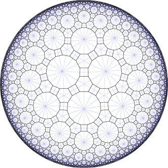
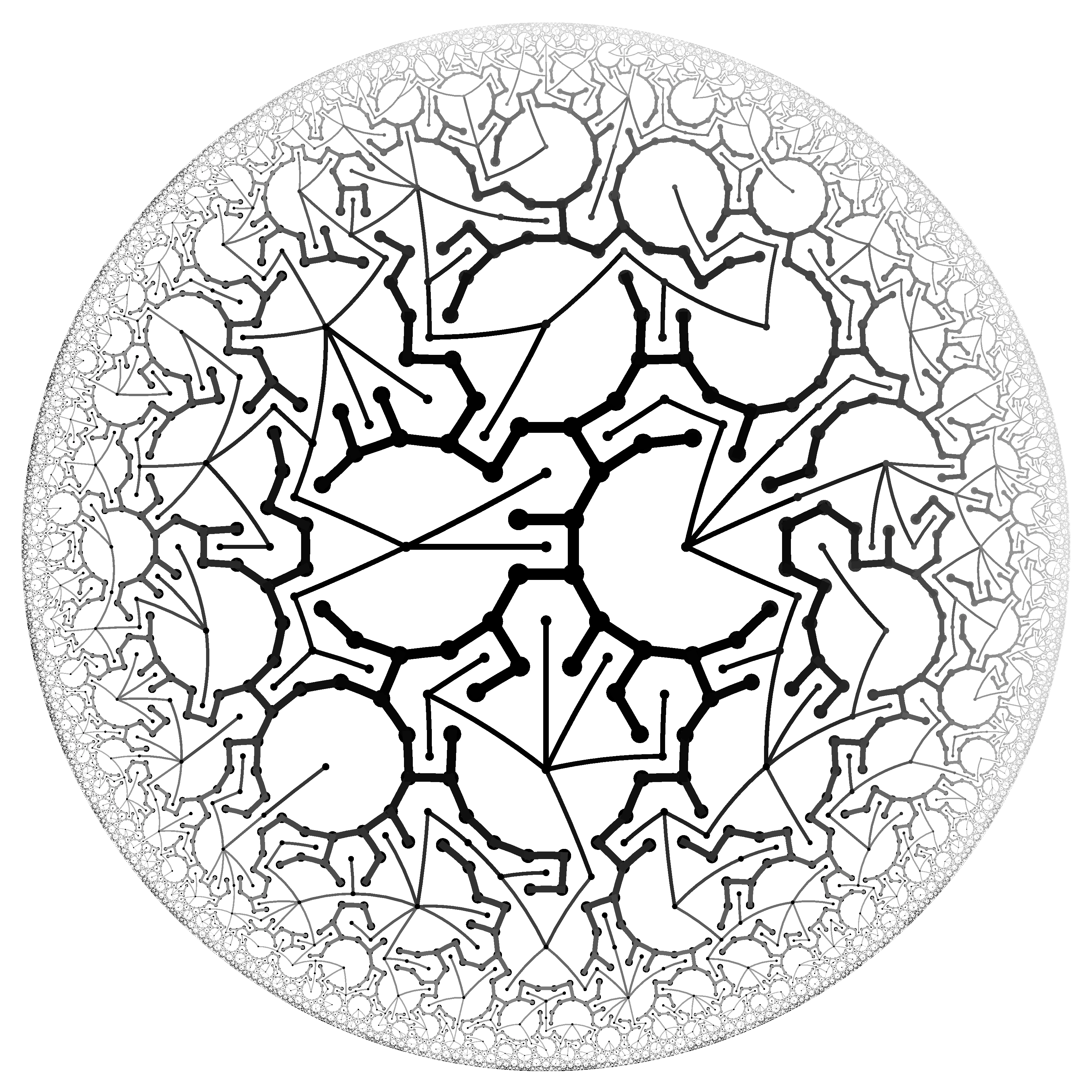
In this section, we show how to compute the looping rate and sandpile density for periodic planar lattices. To a large extent, the formulas for the infinite lattices follow from the finite-graph formulas, but some care is needed when taking the limit where the graph tends to the infinite lattice. For example, there are hyperbolic planar lattices, such as the one shown in Figure 7, for which there is more than one uniform spanning tree measure, and more than one infinite sandpile measure. For finite graphs approximating the hyperbolic lattice, in a certain sense the boundary is too big to be negligible, and different boundary conditions lead to different limiting uniform spanning forest measures and different sandpile measures. To make sense of quantities such as “the sandpile density,” we would like to know that there is only one canonical infinite sandpile measure.

Figure 7: A hyperbolic planar lattice with its dual lattice (left), and a “wired” uniform spanning forest on one lattice together with its dual “free” uniform spanning forest on the dual lattice (right). (The left figure was made by Don Hatch’s HyperbolicApplet program, the right figure was made by Russell Lyons [26, Figs. 6.1 and 10.3].)

Here we shall limit our attention to $\mathbb{Z}^{2}$-periodic connected planar graphs in which the fundamental domain has a finite number of vertices. Each of the lattices listed in Table 1 is of this type. Graphs of this type are recurrent (which follows e.g., from Rayleigh monotonicity [11]). Any recurrent graph has a unique limiting uniform spanning forest measure, and almost surely the spanning forest contains a single tree [2].

Since the uniform spanning forest on the dual lattice is also unique and almost surely contains a single tree, it follows that the spanning tree on the primal lattice almost surely has one end, i.e., almost surely it does not contain a doubly infinite path.

Whenever the uniform spanning forest almost surely contains a single tree with one end, it is clear that there is a unique limiting sandpile measure that results from exploring the tree. (In cases where the spanning forest contains multiple trees, depending on the details of the tree exploration process near the boundary, the USF trees could be explored in different orders, resulting in different sandpiles. However, using a carefully selected tree exploration rule, Járai and Werning showed that whenever the USF almost surely contains one-ended trees, there is a unique limiting sandpile measure [16].)

Let $\mathcal{G}_{n}$ be the graph obtained from the $\mathbb{Z}^{2}$-periodic lattice by merging all vertices outside an $n\times n$ block of fundamental domains (this gives “wired boundary conditions”). The sequence of graphs $(\mathcal{G}_{n})_{n\geq 1}$ converges to the lattice in the sense of Benjamini and Schramm [3], which is to say that for any distance $j>0$, the $j$-neighborhood of a random vertex of $\mathcal{G}_{n}$ converges in distribution as $n\to\infty$ to the $j$-neighborhood of a random vertex in the fundamental domain. (In contrast, the hyperbolic lattice is not a Benjamini-Schramm limit of planar graphs [3].) Since the USF in the lattice has one tree, the spanning tree path connecting two random vertices in $\mathcal{G}_{n}$, when restricted to a neighborhood of one of the vertices, converges in law to the LERW from a random vertex in the lattice to $\infty$. In particular, the looping rate of $\mathcal{G}_{n}$ converges to the looping rate of the lattice, as does the distribution of the erased LERW loops. Comparing the tree exploration process on $\mathcal{G}_{n}$ to that on the lattice, since almost surely the USF on the lattice has one tree with one end, the distribution of sand around a random vertex of $\mathcal{G}_{n}$ converges to the distribution of sand around a random vertex of the lattice, and since the sand at each vertex of $\mathcal{G}_{n}$ is bounded, the rare vertices of $\mathcal{G}_{n}$ with atypical neighborhoods can be ignored, and the density of sand of $\mathcal{G}_{n}$ converges to the lattice sandpile density. Consequently, the finite graph formulas relating the LERW looping rate and other graph parameters also hold in the setting of $\mathbb{Z}^{2}$-periodic lattices.

Furthermore, since the USF is unique and almost surely has a single one-ended tree, (5) implies that there is a unique limit as $n\to\infty$ for the current flowing across any edge in the lattice. Consequently the voltage drop $A^{(s)}_{u,v}$ has a unique limit, which we call the potential kernel. Since it is unique, the potential kernel inherits all the symmetries of the lattice.

We compute $\tau$ using (8). For unweighted lattices, we do not explicitly compute $\rho$, since $\rho-\tau$ is expressible in terms of the average degree $\delta$ via (3) and (4). For weighted lattices, we compute $\rho$ using (3) and (7).

At this point we can start calculating. For the square lattice, by symmetry the potential kernel across neighboring vertices is $1/4$, so for its dual, also the square lattice, we have

$$\tau\text{(square)}=\frac{1}{4}\times\frac{1}{4}+\left(\frac{1}{4}-\frac{1}{4}\right)^{2}=\frac{1}{16}\,.$$

For the triangular lattice, the dual is the honeycomb lattice, for which by symmetry the current flowing across edges is $1/3$,

$$\tau\text{(triangular)}=\frac{1}{3}\times\frac{1}{3}+\left(\frac{1}{3}-\frac{1}{3}\right)^{2}=\frac{1}{9}\,.$$

For the honeycomb lattice, the dual is the triangular lattice, and we have

$$\tau\text{(honeycomb)}=\frac{1}{6}\times\frac{1}{6}+\left(\frac{1}{6}-\frac{1}{6}\right)^{2}=\frac{1}{36}\,.$$

Figure 8: Triangular and honeycomb lattices.

Figure 9: Kagomé and dice lattices.

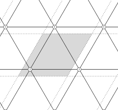
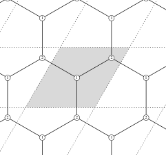
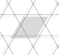
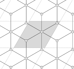
For the dice lattice (Figure 9), the dual is the kagomé lattice, for which the potential kernel across edges is $1/4$ for each edge, and we have

$$\tau\text{(dice)}=\frac{1}{4}\times\frac{1}{4}+\left(\frac{1}{4}-\frac{1}{4}\right)^{2}=\frac{1}{16}\,.$$

The square, triangular, honeycomb, and dice lattices are all sufficiently symmetric that $\tau=1/(\delta^{*})^{2}$. For general unweighted finite planar graphs, (8) together with the bound $a^{2}-ab+b^{2}=\frac{1}{4}(a+b)^{2}+\frac{3}{4}(a-b)^{2}\geq\frac{1}{4}(a+b)^{2}$ imply

$$\tau\geq\sum_{e^{*}}\frac{\frac{1}{4}\Pr[e^{*}\in T^{*}]^{2}}{|E^{*}|}\geq\frac{|E^{*}|((|V^{*}|-1)/|E^{*}|)^{2}}{4|E^{*}|}\,,$$

and hence $\tau\geq 1/(\delta^{*})^{2}$ and also $\lambda\leq 2\delta^{*}$ for unweighted $\mathbb{Z}^{2}$-periodic planar lattices. These bounds are all equalities for the square, honeycomb, triangular, and dice lattices, and appear to be fairly good when each face of the lattice has the same number of sides.

For the kagomé lattice, the dual is the dice lattice (see Figure 9), for which there are two types of vertices (degree-$3$ and degree-$6$), but only one type of edge. By symmetry, for each edge $(u,v)$, the potential kernel $A_{u,v}$ is $1/\operatorname{degree}(u)$. Hence

$$\tau\text{(kagom\'{e})}=\frac{1}{6}\times\frac{1}{3}+\left(\frac{1}{6}-\frac{1}{3}\right)^{2}=\frac{1}{12}\,.$$

The next pair of lattices that we consider are the Fisher lattice (i.e., the truncated hexagonal lattice) and its dual, the triakis triangular lattice (see Figure 10). There are several ways to determine the potential kernel for adjacent vertices of these lattices; we describe a way which essentially only uses symmetry. In the triakis triangular lattice, for the degree-3 vertices the potential kernel is of course $1/3$, by symmetry. Each degree-12 vertex $o$ is surrounded by 6 other degree-12 vertices which are symmetric to one another; let $a$ denote one such vertex. It is also surrounded by 6 degree-3 vertices which are symmetric to one another; let $b$ denote one such vertex. The potential kernel $A_{u,v}$ is harmonic as a function of $v$ except at $u$. Vertex $b$ is surrounded by $o$ and two degree-12 neighbors of $o$. By harmonicity and symmetry, $A_{o,b}=\frac{1}{3}A_{o,o}+\frac{1}{3}A_{o,a}+\frac{1}{3}A_{o,a}=\frac{2}{3}A_{o,a}$. Thus $1=6\times A_{o,a}+6\times A_{o,b}=10A_{o,a}$, so $A_{o,a}=\frac{1}{10}$ and $A_{o,b}=\frac{1}{15}$. Next we use the following relation (14) between the potential kernels of a graph and its dual:

$$w_{u,v}\big{(}A^{(s)}_{u,v}+A^{(s)}_{v,u}\big{)}+w_{u^{*},v^{*}}\big{(}A^{(s^{*})}_{u^{*},v^{*}}+A^{(s^{*})}_{v^{*},u^{*}}\big{)}=1\quad\text{(planar undirected graphs)}.$$ (14)

This follows from (6) because either edge $(u,v)$ is in the tree, or its dual edge $(u^{*},v^{*})$ is in the dual tree. Together with the symmetry in the Fisher lattice, we find that the potential kernel along intertriangle edges is $\frac{1}{2}(1-\frac{1}{10}-\frac{1}{10})=\frac{2}{5}$. For the intratriangle edges, we again use symmetry to find that the potential kernel is $\frac{1}{2}(1-\frac{2}{5})=\frac{3}{10}$.

Figure 10: Fisher lattice and its dual, the triakis triangular lattice.

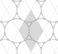
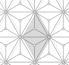
For the triakis triangular lattice, the 3–12 edges are twice as numerous as the 12–12 edges. Thus, for its dual the Fisher lattice, we obtain

$$\tau\text{(Fisher)}=\frac{1}{3}\left[\frac{1}{10}\times\frac{1}{10}+\left(\frac{1}{10}-\frac{1}{10}\right)^{2}\right]+\frac{2}{3}\left[\frac{1}{3}\times\frac{1}{15}+\left(\frac{1}{3}-\frac{1}{15}\right)^{2}\right]=\frac{59}{900}\,.$$

For the Fisher lattice, the intratriangle edges are twice as numerous as the intertriangle edges. Thus, for its dual the triakis triangular lattice, we obtain

$$\tau\big{(}\parbox{0.0pt}{\centering triakis\\ triangular\@add@centering}\big{)}=\frac{1}{3}\left[\frac{4}{10}\times\frac{4}{10}\right]+\frac{2}{3}\left[\frac{3}{10}\times\frac{3}{10}\right]=\frac{17}{150}\,.$$

There are two types of edges in these lattices, and it is natural to give them different edge weights. If we give weight $\beta$ to the edges connecting two degree-12 vertices of the triakis triangular lattice, and weight $1$ to the other edges, then the same symmetry argument can be used to compute the potential kernel. This leads to

$$\tau\big{(}\parbox{0.0pt}{\centering triakis\\ triangular\@add@centering}\big{)} =\frac{2\beta^{3}+8\beta^{2}+6\beta+1}{2(\beta+2)(3\beta+2)^{2}}\,,\text{ and}$$

$$\rho\big{(}\parbox{0.0pt}{\centering triakis\\ triangular\@add@centering}\big{)} =\frac{(\beta+1)(5\beta^{2}+11\beta+5)}{2(\beta+2)(3\beta+2)^{2}}\,.$$

With $\beta=1$ we recover the parameters for the unweighted triakis triangular lattice. Since a random walk on the weighted triakis triangular lattice converges to a random walk on the dice lattice as $\beta\to 0$, and to a random walk on the triangular lattice as $\beta\to\infty$, we can recover $\tau$ and $\rho$ for the dice and triangular lattices by taking these limits. There are similar rational function formulas for $\tau$ and $\rho$ on the weighted Fisher lattice, but it is not as simple to recover the parameters for the honeycomb and kagomé lattices.

The last pair of periodic lattices we consider are the square-octagon lattice (i.e., the truncated square lattice), and its dual the tetrakis square lattice (see Figure 11). Since there are two edge types, we give the edges connecting degree-8 vertices in the tetrakis square lattice an edge weight of $\beta$, or equivalently, we give the edges between octagons in the square-octagon lattice weight $1/\beta$. In the tetrakis square lattice, the potential kernel between a degree-4 vertex and one of its neighbors is $\frac{1}{4}$ by symmetry. Let $\alpha=\alpha(\beta)$ denote the potential kernel between two adjacent degree-8 vertices. Then the potential kernel from a degree-8 to a degree-4 vertex is $\frac{1}{4}-\alpha\beta$. For the square-octagon lattice, we use Equation (14) relating the potential kernel of a graph to that of its dual together with the bilateral symmetry of the edges to deduce that for the intersquare edges the potential kernel is $\frac{1}{2}\beta(1-\alpha\beta-\alpha\beta)=\frac{1}{2}\beta-\alpha\beta^{2}$, from which it follows that the potential kernel for the edges in the squares is $\frac{1}{4}+\alpha\beta/2$. Substituting these values into Equations (8), (3), and (7), and using the fact that the unweighted edges are twice as numerous as the weighted ones, we obtain

Figure 11: Square-octagon lattice and its dual, the tetrakis square lattice.

$$\tau\big{(}\parbox{0.0pt}{\centering tetrakis\\ square\@add@centering}\big{)} =\frac{\tfrac{1}{4}\beta+\tfrac{1}{8}}{\beta+2}-\frac{\beta-\tfrac{1}{2}}{\beta+2}\beta\alpha+\frac{\beta+\tfrac{1}{2}}{\beta+2}\beta^{2}\alpha^{2}\,,$$

$$\rho\big{(}\parbox{0.0pt}{\centering tetrakis\\ square\@add@centering}\big{)} =\frac{\tfrac{1}{4}\beta+\tfrac{5}{8}}{\beta+2}-\frac{\tfrac{3}{2}}{\beta+2}\beta\alpha+\frac{\beta+\tfrac{1}{2}}{\beta+2}\beta^{2}\alpha^{2}\,,$$

and

$$\tau\big{(}\parbox{0.0pt}{\centering square-\\ octagon\@add@centering}\big{)} =\frac{\tfrac{1}{8}\beta}{1+2\beta}-\frac{\tfrac{1}{2}\beta}{1+2\beta}\beta\alpha+\beta^{2}\alpha^{2}\,,$$

$$\rho\big{(}\parbox{0.0pt}{\centering square-\\ octagon\@add@centering}\big{)} =\frac{\tfrac{5}{8}\beta+\tfrac{1}{2}}{1+2\beta}+\frac{\tfrac{1}{2}\beta-1}{1+2\beta}\beta\alpha+\beta^{2}\alpha^{2}\,.$$

Symmetry is not enough to determine the value of $\alpha$, but we can use a method that is applicable to any periodic graph [38]. We write the Laplacian in Fourier space as a matrix $\widehat{\Delta}(z,w)$ indexed by the vertices of a fundamental domain. An edge connecting a vertex of type $i$ to a vertex of type $j$ in the fundamental domain $x$ units in the $z$-direction and $y$ units in the $w$-direction contributes $1$ to $\Delta_{i,i}$ and $-z^{x}w^{y}$ to $\Delta_{i,j}$. The tetrakis square lattice’s fundamental domain has two vertices, and in this case we have

$$\widehat{\Delta}(z,w)=\begin{bmatrix}4&-\frac{1}{wz}{-}\frac{1}{w}{-}\frac{1}{z}{-}1\\[4.0pt] -wz{-}w{-}z{-}1&4{+}4\beta{-}\beta w{-}\frac{\beta}{w}{-}\beta z{-}\frac{\beta}{z}\end{bmatrix}\,.$$

The Green’s function is given by the inverse Fourier transform of $\widehat{G}(z,w)=\widehat{\Delta}^{-1}(z,w)$, that is a double integral over the circle of a rational function in $z$ and $w$. The potential kernel $A_{u,v}$ between a vertex $u$ of type $i$ and a vertex $v$ of type $j$ in a fundamental domain shifted by $x$ units in the $z$-direction and $y$ units in the $w$-direction is

$$A_{u,v}=\oint\!\!\oint\left[\big{(}\widehat{\Delta}(z,w)^{-1}\big{)}_{i,i}-\frac{\big{(}\widehat{\Delta}(z,w)^{-1}\big{)}_{i,j}}{z^{x}w^{y}}\right]\frac{dz}{2\pi iz}\,\frac{dw}{2\pi iw}\,.$$

The evaluation of $\alpha$ corresponds to the case $i=j=2$, and by symmetry $(x,y)$ can be any of $(1,0)$, $(-1,0)$, $(0,1)$, or $(0,-1)$. Also $\big{(}\widehat{\Delta}(z,w)^{-1}\big{)}_{2,2}=4/P(z,w)$, where

$$P(z,w)=16\beta+12-(4\beta+2)(z+z^{-1}+w+w^{-1})-(z+z^{-1})(w+w^{-1})\,.$$

Using symmetry, we can average the integrals for $(x,y)=(0,1)$ and $(x,y)=(0,-1)$:

$$\alpha=2\oint\!\!\oint\frac{2-w-w^{-1}}{P(z,w)}\,\frac{dz}{2\pi iz}\,\frac{dw}{2\pi iw}\,.$$

Now for $b<1$

$$\oint\frac{1}{1+b(z+z^{-1})/2}\frac{dz}{2\pi iz}=\frac{1}{\sqrt{1-b^{2}}}\,,$$

so

$$\alpha=2\oint\frac{2-w-w^{-1}}{\sqrt{(16\beta+12-(4\beta+2)(w+w^{-1}))^{2}-4(4\beta+2+w+w^{-1})^{2}}}\,\frac{dw}{2\pi iw}\,,$$

which after changing variables letting $w=e^{2\pi it}$ and simplifying gives

$$\alpha=\frac{1}{2\sqrt{\beta^{2}+\beta}}\int_{0}^{1}\sqrt{\frac{1-\cos(2\pi t)}{(3+2/\beta)-\cos(2\pi t)}}\,dt\,.$$

Now $1-\cos(2\pi t)=2\sin^{2}(\pi t)$. Let $u=\sin(\pi t)$. Then $dt=du/(\pi\sqrt{1-u^{2}})$, so

$$\alpha=\frac{1}{\pi\sqrt{\beta^{2}+\beta}}\int_{0}^{1}\sqrt{\frac{u^{2}}{(1+1/\beta)+u^{2}}}\,\frac{du}{\sqrt{1-u^{2}}}\,.$$

Let $(2+1/\beta)v^{2}=1-u^{2}$, so $(2+1/\beta)v\,dv=-u\,du=\sqrt{2+1/\beta}\sqrt{1-u^{2}}\,dv$, and

$$\alpha=\frac{1}{\pi\sqrt{\beta^{2}+\beta}}\int\limits_{\frac{1}{\sqrt{2+1/\beta}}}^{0}\frac{-dv}{\sqrt{1-v^{2}}}=\frac{\arcsin\big{(}1/\sqrt{2+1/\beta}\big{)}}{\pi\sqrt{\beta^{2}+\beta}}\,.$$

The sine-doubling formula gives

$$2\arcsin\left(\frac{1}{\sqrt{2+1/\beta}}\right) =\arcsin\left(2\sqrt{\frac{1}{2+1/\beta}}\sqrt{\frac{1+1/\beta}{2+1/\beta}}\right)$$

$$=\arcsin\sqrt{1-\frac{1/\beta^{2}}{(2+1/\beta)^{2}}}=\operatorname{arcsec}(2\beta+1)\,,$$

so

$$\alpha=\alpha(\beta)=\frac{\operatorname{arcsec}(2\beta+1)}{2\pi\sqrt{\beta^{2}+\beta}}\,.$$

For every rational value of the edge weight $\beta$ except $\frac{1}{2}$, the number $\alpha(\beta)$ is transcendental. (The exceptional point is $\alpha(\frac{1}{2})=1/\sqrt{27}$.) This follows from the Gelfond-Schneider theorem (see [31, Chapt. 10]) together with the result that for rational $r$, the only rational values of $\cos(r\pi)$ are $0,\pm 1,\pm\frac{1}{2}$ (see [31, Cor. 3.12]). Consequently the sandpile density (and the parameters $\tau$ and $\rho$) are transcendental for $\beta\in\mathbb{Q}^{+}\setminus\{\frac{1}{2}\}$.

8 Open problems

On the infinite branching tree with degree $\delta$ (and wired boundary conditions), the sandpile density is $\delta/2$ [10]. It would be interesting if the (wired) sandpile density could be computed for other planar hyperbolic lattices.

The variance in the amount of sand of a recurrent sandpile configuration is the variance in its level. Expressing this in terms of the binomial moments and using (12) and planar duality, the variance is

$$2\frac{F_{3}(\mathcal{G}^{*})}{F_{1}(\mathcal{G}^{*})}+\frac{F_{2}(\mathcal{G}^{*})}{F_{1}(\mathcal{G}^{*})}-\left(\frac{F_{2}(\mathcal{G}^{*})}{F_{1}(\mathcal{G}^{*})}\right)^{2},$$ (15)

where the forest formula [25, 30] gives

$$\frac{F_{k}(\mathcal{G})}{F_{1}(\mathcal{G})}=\sum_{h=0}^{k-1}(-1)^{h}\!\!\!\!\!\!\sum_{\begin{subarray}{c}\{u_{1}\sim v_{1},\dots,u_{h}\sim v_{h}\}\subset E\\ \{x_{1},\dots,x_{k-1-h}\}\subset V\end{subarray}}\!\!\!w_{u_{1},v_{1}}\cdots w_{u_{h},v_{h}}\det G_{u_{1},v_{1},\dots,u_{h},v_{h},x_{1},\dots,x_{k-1-h}}^{u_{1},v_{1},\dots,u_{h},v_{h},x_{1},\dots,x_{k-1-h}}$$ (16)

where the inner sum is over sets of $h$ undirected edges and sets of $k-1-h$ vertices. For the square grid, the variance in the amount of sand in a random recurrent sandpile configuration of an $n\times n$ box in $\mathbb{Z}^{2}$ appears to be $(0.14386408549334\dots+o(1))\times n^{2}$. Is there a closed-form expression for this asymptotic variance? Is the total amount of sand distributed according to a Gaussian?

For non-planar graphs, what is the complexity of counting spanning unicyclic subgraphs? Is it #P-hard? Is it polynomial time solvable? Is there a good formula which can be used to find the sandpile density?

• studied mathematics at École Normale Supérieure in Paris from 2006 to 2010. He obtained a doctoral degree in mathematics from Université Paris Sud in 2013.

  • ETH Zürich, Departement Mathematik, Rämistrasse 101, 8092 Zürich, Switzerland
    adrien.kassel@math.ethz.ch

• graduated from MIT in 1991 with degrees in electrical engineering, math, and computer science, and graduated again from MIT with a Ph.D. in math in 1996. He specializes in probability and algorithms, and has a longtime interest in trees and sand.

  • Microsoft Research, One Microsoft Way, Redmond, WA 98052, U.S.A.
    http://dbwilson.com

References

- 1. P. Bak, C. Tang, and K. Wiesenfeld, Self-organized criticality, Phys. Rev. A (3) 38 (1988), 364–374.
- 2. I. Benjamini, R. Lyons, Y. Peres, and O. Schramm, Uniform spanning forests, Ann. Probab. 29 (2001), 1–65.
- 3. I. Benjamini and O. Schramm, Recurrence of distributional limits of finite planar graphs, Electron. J. Probab. 6 (2001), no. 23, 13 pp.
- 4. O. Bernardi, Tutte polynomial, subgraphs, orientations and sandpile model: new connections via embeddings, Electron. J. Combin. 15 (2008), #R109.
- 5. R. Burton and R. Pemantle, Local characteristics, entropy and limit theorems for spanning trees and domino tilings via transfer-impedances, Ann. Probab. 21 (1993), 1329–1371.
- 6. S. Caracciolo and A. Sportiello, Exact integration of height probabilities in the abelian sandpile model, J. Stat. Mech. Theory Exp. (2012), P09013.
- 7. S. Chaiken, A combinatorial proof of the all minors matrix tree theorem, SIAM J. Algebraic Discrete Methods 3 (1982), 319–329.
- 8. R. Cori and Y. Le Borgne, The sand-pile model and Tutte polynomials, Adv. in Appl. Math. 30 (2003), 44–52.
- 9. D. Dhar, Self-organized critical state of sandpile automaton models, Phys. Rev. Lett. 64 (1990), 1613–1616.
- 10. D. Dhar and S. N. Majumdar, Abelian sandpile model on the Bethe lattice, J. Phys. A 23 (1990), 4333–4350.
- 11. P. G. Doyle and J. L. Snell, Random walks and electric networks, Carus Mathematical Monographs #22, Mathematical Association of America, 1984.
- 12. A. M. Duval, C. J. Klivans, and J. L. Martin, Simplicial matrix-tree theorems, Trans. Amer. Math. Soc. 361 (2009), 6073–6114.
- 13. R. Forman, Determinants of Laplacians on graphs, Topology 32 (1993), 35–46.
- 14. A. E. Holroyd, L. Levine, K. Mészáros, Y. Peres, J. Propp, and D. B. Wilson, Chip-firing and rotor-routing on directed graphs, In and out of equilibrium 2, Progress in Probability #60, Birkhäuser, 2008, pp. 331–364. http://arxiv.org/abs/0801.3306
- 15. A. A. Járai, Sandpile models, (2014), Cornell probability summer school lecture notes. http://arxiv.org/abs/1401.0354.
- 16. A. A. Járai and N. Werning, Minimal configurations and sandpile measures, J. Theoret. Probab. 27 (2014), 153–167.
- 17. M. Jeng, G. Piroux, and P. Ruelle, Height variables in the abelian sandpile model: scaling fields and correlations, J. Stat. Mech. (2006), P10015.
- 18. G. Kalai, Enumeration of -acyclic simplicial complexes, Israel J. Math. 45 (1983), 337–351.
- 19. R. Kenyon, Spanning forests and the vector bundle Laplacian, Ann. Probab. 39 (2011), 1983–2017.
- 20. R. W. Kenyon and D. B. Wilson, Spanning trees of graphs on surfaces and the intensity of loop-erased random walk on planar graphs, J. Amer. Math. Soc. (forthcoming), http://arxiv.org/abs/1107.3377.
- 21. G. Kirchhoff, Ueber die Auflösung der Gleichungen, auf welche man bei der Untersuchung der linearen Vertheilung galvanischer Ströme geführt wird, Ann. Phys. und Chem. 72 (1847), no. 12, 497–508.
- 22. G. F. Lawler and V. Limic, Random walk: A modern introduction, Cambridge Studies in Advanced Mathematics #123, Cambridge Univ. Press, 2010.
- 23. G. F. Lawler, O. Schramm, and W. Werner, Conformal invariance of planar loop-erased random walks and uniform spanning trees, Ann. Probab. 32 (2004), 939–995.
- 24. L. Levine and Y. Peres, The looping constant of , Random Structures Algorithms 45 (2014), 1–13.
- 25. C. J. Liu and Y. Chow, Enumeration of forests in a graph, Proc. Amer. Math. Soc. 83 (1981), 659–662.
- 26. R. Lyons (with Y. Peres), Probability on trees and networks, Cambridge Univ. Press, book in preparation. http://mypage.iu.edu/~rdlyons/prbtree/.
- 27. S. N. Majumdar and D. Dhar, Height correlations in the abelian sandpile model, J. Phys. A: Math. Gen. 24 (1991), L357.
- 28. S. N. Majumdar and D. Dhar, Equivalence between the abelian sandpile model and the limit of the Potts model, Physica A 185 (1992), 129–145.
- 29. C. Merino López, Chip firing and the Tutte polynomial, Ann. Comb. 1 (1997), 253–259.
- 30. W. Myrvold, Counting -component forests of a graph, Networks 22 (1992), 647–652.
- 31. I. Niven, Irrational numbers, Carus Mathematical Monographs #11, Mathematical Association of America, 1956.
- 32. R. Pemantle, Choosing a spanning tree for the integer lattice uniformly, Ann. Probab. 19 (1991), 1559–1574.
- 33. V. S. Poghosyan and V. B. Priezzhev, The problem of predecessors on spanning trees, Acta Polytechnica 51 (2011), 59–62.
- 34. V. S. Poghosyan, V. B. Priezzhev, and P. Ruelle, Return probability for the loop-erased random walk and mean height in sandpile: a proof, J. Stat. Mech. (2011), P10004.
- 35. V. B. Priezzhev, Exact height probabilities in the abelian sandpile model, Phys. Scr. T49 (1993), 663–669.
- 36. , Structure of two-dimensional sandpile. I. Height probabilities, J. Stat. Phys. 74 (1994), 955–979.
- 37. O. Schramm, Scaling limits of loop-erased random walks and uniform spanning trees, Israel J. Math. 118 (2000), 221–288.
- 38. F. Spitzer, Principles of random walks, second edition, Graduate Texts in Mathematics #34, Springer-Verlag, 1976.
- 39. H. N. V. Temperley, Graph theory and applications, Ellis Horwood Series in Mathematics and its Applications, John Wiley & Sons, 1981.
- 40. D. B. Wilson, Generating random spanning trees more quickly than the cover time, Proc. 28th Annual ACM Symposium on the Theory of Computing, 1996, pp. 296–303.
- 41. D. Zeilberger, A combinatorial approach to matrix algebra, Discrete Math. 56 (1985), 61–72.
-
ADRIEN KASSEL