On Simulation of Various Effects in Consolidated Order Book.

Abstract.

This paper consists of two parts. The first part is devoted to empirical analysis of consolidated order book (COB) for the index RTS futures. In the second part we consider Poissonian multi–agent model of the COB. By varying parameters of different groups of agents submitting orders to the book we are able to model various real life phenomenas. In particular we model the spread, the profile of the book and large price changes. Two different mechanisms of large price changes are considered in detail. One is the disbalance of liquidity in the COB and another is the disbalance of sell and buy orders in the order flow.

1. Introduction.

Price changes and its causes been a classical topic of economics research for a long time already. The answer to the traditional question ”why prices change” in the theory of effective market is that the market absorbs a new information which forces market participants to reconsider the price of securities, currencies, futures, etc.

At the level of micro–structure investigation of a price change became possible only after historical data about all orders and events in the exchange became publicly available. For a novice in the field we say that the order matching mechanism of an exchange is called consolidated order book (COB) or simply the book. In this work we do not consider the causes that determine the rate of submitting limit and market orders to the book by market participants. Instead the main emphases is made on a study of various book statistics and a price changing mechanisms. In this work we assume that all rates are constant in time i.e. we stay in the realm of ”zero” intelligence traders, [5].

It turns out that there are two basic mechanisms of the price change. In one case it is the disbalance between demand through the flow of market orders and supply of limit orders in the book. Nevertheless, the simple rule telling us what is happening if the demand exceeds supply not necessarily leads to a price change. Another cause of the price change is the disbalance of liquidity in the order book. In reality two of these mechanisms contribute in a certain combination.

Our work consists of two parts. The first part is devoted to study of empirical statistics of the book and the order flow for futures on the RTS index. Similar investigation was previously performed on stocks traded on French and USA equity exchanges [1] and [2]. The Russian Trading System (RTS) is a stock market established in 1995 in Moscow, consolidating various regional trading floors into one exchange. Originally RTS was modeled on NASDAQ’s trading and settlement framework. The RTS Index, RTSI, the official Exchange indicator, first calculated on September 1, 1995, is similar to the Dow Jones Index. Nowadays the value of contracts traded in RTS Index futures and options exceeded tens of billion dollars. The number of open positions (open interest) exceeds 250,000 contracts. The excellent liquidity allows us to compute various statistics of the order book from historical data provided by RTS.

The second part of this work contains simulations performed with the use of the Poissonian multi–agent model of the order book. For the first time Poissonian models were considered by J.D. Farmer at all in [10, 11, 12]. We formulate our model using multi–agent framework [4, 7]. We presents results of numerical simulations which are similar to real statistics of the RTS index futures. We have to mention that some of these simulations already appeared in [6]. The limiting case of the model corresponding to the book of density one was rigorously considered by us in [8] and [9].

For convenience of the reader we start our presentation with detailed description of the order book.

2. The Order Book.

In this work we consider an exchange with continuous double auction as the order matching mechanism. Market participants submit to the exchange orders of two types, namely limit orders and market orders.

The limit orders are specified by three parameters, the price level, the volume and the direction (buy or sell). The price is the worst price at which the order can be executed. The volume of an order is a number of contracts which constitute the order.

The consolidated order book is shown in Figure 1. The mid–column is a price ladder for a security. Each limit order is placed in the order book at the level specified by its price. The minimal price to sell is called an ask price and the maximal price to buy is called a bid price. The first column represents a price level counted from the best ”bid” price. The second ”bid” column represents a total volume of orders that can be bought at the specific price. On the right from the middle column the situation is identical but reversed. The fourth column is the total volume of orders at the specific price level. The last the fifth column is a price level counted from the best ”ask”.

Figure 1. Consolidated Order Book

Limit order stay in the book until they get executed or just canceled. Execution of orders in each queue is determined by the FIFO rule i.e. First In, First Out.

The price level for ”buy” orders is counted from the best price offer (ask price) at the moment

$$l(p)=\frac{p_{ask}-p}{s},\qquad\qquad p<p_{ask};$$

where $p_{ask}$ is the best price to buy and $s$ is the size of the price ladder step. Similarly the price level for ”sell” orders is counted from the best price offer (bid price)

$$l(p)=\frac{p-p_{bid}}{s},\qquad\qquad p>p_{bid};$$

where $p_{bid}$ is the best price to sell.

The state of the book is given by a vector $X=\{x_{i}\}$, where $|x_{i}|$ is aggregated volume of orders at level $i$. The component $x_{i}$ is positive if these are buy orders and negative if these are sell orders. Note that

$$i=\frac{price}{s},\quad\quad\quad i_{ask}=\frac{p_{ask}}{s},\quad\quad\quad i_{bid}=\frac{p_{bid}}{s}.$$

We define instant liquidity to sell as

$$s(l)=\sum_{i=i_{ask}}^{i_{ask}+l}X_{i},\quad\quad s=s(\infty);$$

and instant liquidity to buy as

$$d(l)=\sum_{i=i_{bid}}^{i_{bid}-l}X_{i},\quad\quad d=d(\infty).$$

Market orders are the orders which have no specific price and the only volume is specified. Such orders are executed at the best available price at the moment they are submitted. If, for example, in the book shown in Fig 1 submitted a market order to buy of the size 70, then the part of it (68 orders) is executed at the price 150005 and the remaining 2 orders are executed at the price 150010.

3. The Empirical Statistics of the RTS Futures Order Book.

3.1. The rate of submitting or canceling orders.

The rate of submitted limit orders $I_{L}(l)$ can be measured from historical data. We used the futures contract on index RTS and represented the rate of submitting limit orders in Figure 2 on the logarithmic scale. The vertical axis represents the number of contracts per second on both buy and sell side and the horizontal axis represents the price level.

Figure 2. The rate $I_{L}(l)$.

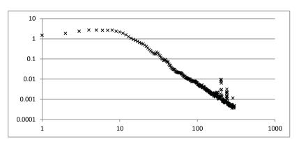
Starting from level ten the order submitting rate follows the power law $I_{L}(l)\sim l^{-\mu}$, $l>10$. For RTS futures $\mu\approx 2.5$.

Similarly the rate of canceling limit orders $I_{C}(l)$ on the logarithmic scale is presented in Figure 3. For level ten and higher the rate of canceling orders follows the power law $I_{C}(l)\sim l^{-\mu}$ with $\mu\approx 2.5$.

Figure 3. The rate $I_{C}(l)$.

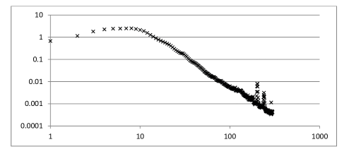
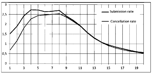
Moreover, $I_{C}(l)=I_{L}(l)$, for $l>10$. At the same time, $I_{C}(l)<I_{L}(l)$ for $l<10$ as shown in Figure 4

Figure 4. The smoothed curves for rates $I_{C}(l)$ and $I_{L}(l).$

3.2. The Order Volume.

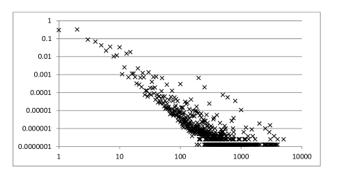
The empirical distribution of market orders volumes $\hat{p}_{M}(\nu)$ is shown in Figure 5. The empirical frequency is depicted on the vertical axis and the volume on the horizontal axis. This distribution can be approximated by the power law $\hat{p}_{M}(\nu)\sim\nu^{-\gamma},\gamma\approx 2.5$.

Figure 5. The empirical distribution $\hat{p}_{M}(\nu)$ of volume of market orders.

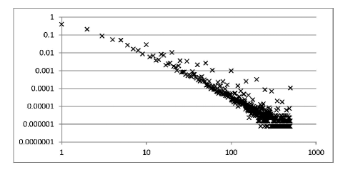
The distribution of limit order volume $\hat{p}_{L}(\nu)$ is more complicated and given in Figure 6. The volume of orders have tendency to be multiple of 10. If one excludes orders with the volume multiple of 10 then $\hat{p}_{L}(\nu)\sim\nu^{-\gamma},\gamma\approx 2.8$. For orders multiple of 10 the distribution is the same with $\gamma\approx 2.5$. For orders multiple of 100 the law is also the same but $\gamma\approx 2.0$.

Figure 6. The empirical distribution $\hat{p}_{L}(\nu)$ of volume of limit orders.

3.3. The Book Profile.

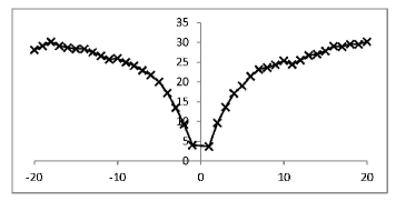
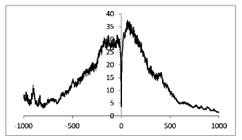
The book profile was determined by averaging the volume at particular level counted from the mid price

$$m=\frac{a_{0}+b_{0}}{2}.$$

The averaged book profile for the first 20 levels is given in Figure 7

Figure 7. The book for the first 20 levels.

The averaged book profile for the first 1000 levels is given in Figure 8

Figure 8. The book for the first 1000 levels.

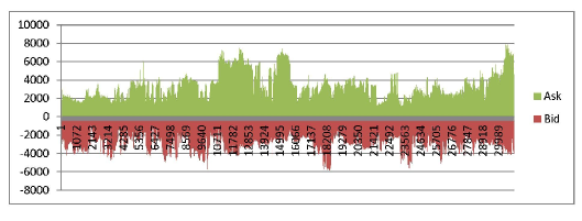
One can look at the time dynamics of the total order volume at first one hundred levels on the sell and buy side. These are exactly the quantities $s(100)$ and $d(100)$ defined above. The volume is measured for each second. The results are presented in Figure 9.

Figure 9. The time dynamics of the aggregated volumes $s(100)$ and $d(100)$.

3.4. The Time Between Orders.

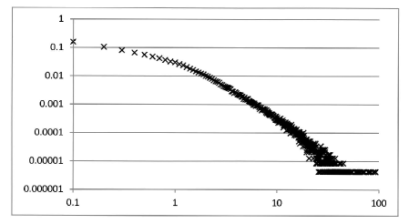
The empirical distribution of time between market orders can measured (in seconds) and is given in Figure 10.

Figure 10. The empirical distribution of time between market orders.

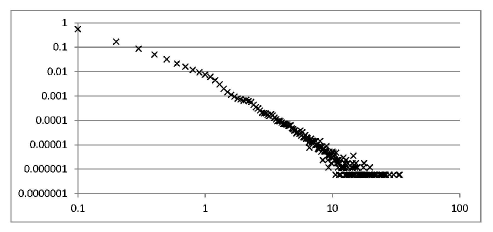
The empirical distribution of time between limit orders can also be measured (in seconds) and is presented in Figure 11

Figure 11. The empirical distribution of time between limit orders.

4. The Poissonian Multi–Agent Model.

4.1. Market Participants

In accordance with a mechanism of the double auction there are six type of events that can occur in the order book

• Liquidity provider submits buy limit order

• Liquidity provider submits sell limit order

• Liquidity taker submits market buy order

• Liquidity taker submits market sell order

• Liquidity taker cancels buy limit order

• Liquidity taker cancels sell limit order

These events can be produced by six agents or market participants. One group are agents providing liquidity to the book and another group are agents taking liquidity from the book.

One group are liquidity providers which differ from each other by a direction of limit orders. Providers of sell liquidity submit sell limit orders to the book and providers of buy liquidity submit buy limit orders to the book.

Another group are liquidity takers. Liquidity takers submit market orders to the book and also differ from each other by a direction. For example, liquidity takers of buy orders send market sell orders to the book. Similarly liquidity takers of sell orders send buy market buy orders. Another type of liquidity takers can cancel active buy or sell limit orders.

Everywhere below we assume that the events in our model form a Poisson flow. Namely the time $\tau$ between two consecutive events is exponentially distributed with the distribution $Prob\,\{\tau\geq t\}=\exp(-It),$ where the parameter $I>0$ is called the rate.

Parameters for providers and takers of $buy$ liquidity we denote with the lower subscript $bid$ and parameters of takers and providers of $sell$ liquidity are denoted with the subscript $ask$. The superscript specifies the type and stands for the following

• $L$ – limit order,

• $M$ – market order,

• $C$ – cancellation of an active limit order in the book.

Every group of market participants acts with the Poisson rate $I^{type}_{side}$ where the subscript stands for the direction and the superscript for the type of action. The total rate of all events in the exchange is given by the formula

$$I=I_{ask}^{L}+I_{bid}^{L}+I_{ask}^{C}+I_{bid}^{C}+I_{ask}^{M}+I_{bid}^{M};$$

where

$I_{bid}^{L}$ – the rate of submitting limit buy orders;

$I_{ask}^{L}$ – the rate of submitting limit sell orders;

$I_{ask}^{M}$ – the rate of submitting market buy orders;

$I_{bid}^{M}$ – the rate of submitting market sell orders;

$I_{ask}^{C}$ – the rate of submitting cancellation request for limit sell orders;

$I_{bid}^{C}$ – the rate of submitting cancellation request for limit buy orders.

On each step of simulation only one of these six events occurs. The time between two consecutive events is exponentially distributed with the rate $I$. The probability of an event is given by the formula

$$\frac{I^{type}_{side}}{I}.$$

For example, the probability of cancellation of some buy limit (bid) order is

$$\frac{I^{C}_{bid}}{I}.$$

4.2. Liquidity providers.

Liquidity providers submit limit orders buy or sell of volume $\nu$ at some price level $l$. Price level $l$ takes also integer values $1,2,\cdots,K;$ with the probability $q^{L}(l).$ We assume also that maximal price level $K=1000$. The distribution function $q^{L}(l)$ is determined by the empirical rate $I_{L}(l)$. The volume $\nu$ of an order takes integer values $1,2,\cdots,V^{L};$ with probability $p^{L}(\nu).$ We assume that maximal volume $V^{L}=1000.$ The distribution $p^{L}(\nu)$ is modeled upon the empirical distribution $\hat{p}^{L}(\nu)$. The distribution functions for the volume and the price level are the same for providers of sell and buy orders.

The limit orders can be executed partially, meaning that if they are bigger then the size of a market order then just some part of them can be filled.

The rate of submitting liquidity i.e. limit orders in the book

$$V_{in}=S^{L}(I_{ask}^{L}+I_{bid}^{L}),$$

where

$$S^{L}=\sum_{\nu=1}^{V^{L}}\nu p^{L}(\nu).$$

4.3. Liquidity takers.

Liquidity takers submit either market orders or just simply cancel existent limit orders in the book. Market orders have a random volume $\nu$ which takes values $1,2,\cdots,V^{M};$ with probability $p^{M}(\nu)$ which is modeled upon the empirical distribution $\hat{p}^{M}(\nu)$. The maximal volume $V^{M}=100$.

4.4. Conditions of equilibrium.

Cancellation of limit orders happens with an equal probability for all active limit orders buy or sell. Let us define

$$S^{C}=\sum_{\nu=1}^{V^{L}}\nu p^{C}(\nu),$$

where $p^{C}(\nu)$ is the distribution function of the volume of canceled limit orders. Active limit orders in the book are subjected to the flow of market orders. Market orders can take limit orders completely or just make the size of limit orders smaller than when they were actually submitted. Therefore,

$$S^{C}<S^{L}.$$

The rate of liquidity consumption

$$V_{out}=S^{M}(I_{ask}^{M}+I_{bid}^{M})+S^{C}(I_{ask}^{C}+I_{bid}^{C}),$$

where

$$S^{M}=\sum_{\nu=1}^{V^{M}}\nu p^{M}(\nu).$$

The quantities $s$ and $d$ determine instant liquidity in the book. The rate of change of instant liquidity is given by

$$\Delta s=I_{ask}^{L}S^{L}-I_{ask}^{M}S^{M}-I_{ask}^{C}S^{C},$$

and

$$\Delta d=I_{bid}^{L}S^{L}-I_{bid}^{M}S^{M}-I_{bid}^{C}S^{C}.$$

Obviously in the stationary regime $\Delta s=\Delta d=0$ and the following identities hold

$$S^{L}I_{ask}^{L}=S^{M}I_{ask}^{M}+S^{C}I_{ask}^{C},$$

$$S^{L}I_{bid}^{L}=S^{M}I_{bid}^{M}+S^{C}I_{bid}^{C}.$$

These imply $V_{in}=V_{out}$.

When market orders are not present $I_{bid}^{M}=I_{ask}^{M}=0$ we have $S^{C}=S^{L}$ and therefore

$$I_{bid}^{L} = I_{bid}^{C},$$

$$I_{ask}^{L} = I_{ask}^{C}.$$

Let us also define aggregated supply of sell orders

$$S=I_{ask}^{L}S^{L}+I_{bid}^{M}S^{M}-I_{ask}^{C}S^{C},$$

and buy orders

$$D=I_{bid}^{L}S^{L}+I_{ask}^{M}S^{M}-I_{bid}^{C}S^{C}.$$

The state of equilibrium is determined by two conditions

• The balance of instantaneous liquidity.

• The balance of rate of change of instant liquidity.

These conditions imply $s=d>0$ and $\Delta s=\Delta d$ which is equivalent to $S=D$. We are going to study price dynamics in terms $s,\,d,\,S,\,D$.

5. Results of Simulation.

We would like to note that sometime during simulation there are no limit orders in the book on sell or buy side. In other words, due to randomness liquidity in the book can drop to zero, meaning $s=0$ or $d=0$. In such case when market order arrives it will be no limit orders in the book to match market order. In order to avoid this we impose the following conditions

$$s>s_{min},\qquad\qquad d>d_{min},$$

where $s_{min}>V^{M}$ and $d_{min}>V^{M}$. Once any of these conditions has been violated we need to stop the flow of market orders and also stop cancellations

$$I_{bid}^{M}=I_{bid}^{C}=0,\qquad\text{if}\quad d<d_{min},$$

or

$$I_{ask}^{M}=I_{ask}^{C}=0,\qquad\text{if}\quad s<s_{min}.$$

Another problem in running simulations is an unlimited growth of a number of limit orders in the book; in other words instant liquidity can not grow indefinitely. We arrange parameters (the rates $I_{side}^{type}$) such that aggregated rate of liquidity supply is less than aggregated rate of liquidity consumption. This implies that the rates have to be such that the following conditions hold

$$\Delta d<0,\qquad\text{for}\quad d>d_{min},$$

and

$$\Delta s<0,\qquad\text{for}\quad s>s_{min}.$$

5.1. The Profile of the Book and the Spread.

Let us define profile of the book as the state of all queues at a particular moment of time. Average profile is computed by averaging instantaneous profiles for each second on a particular time interval.

The response of the book profile to the flow of market orders can be easily understood. When the market orders are absent $I_{bid}^{M}=0$ and $I_{ask}^{M}=0$ all existent orders are canceled without exception and $S_{L}=S_{C}$. This implies that

$$I_{ask}^{L}=I_{ask}^{C},\qquad\qquad\qquad I_{bid}^{L}=I_{bid}^{C}.$$

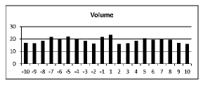
Since in our model the size of limit order is independent from the price and direction of the trade then the the book is filled uniformly with the limit orders as it is shown in Figure 12.

Figure 12. The Book profile without market orders.

Consider now the spread

$$\delta=\frac{p_{ask}-p_{bid}}{s},$$

and let us study how its depends on the size of a market order.

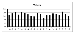
When the market orders submission rate is small

$$\frac{I_{ask}^{M}}{I}<0.01,\quad\quad\quad\quad\quad\quad\frac{I_{bid}^{M}}{I}<0.01,$$

then the book profile remains unchanged as shown in Figure 13

Figure 13. The Book profile with small rate of market orders.

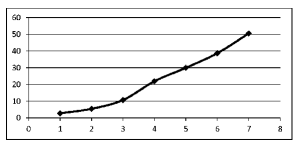
The spread (after the market order has been executed) depends linearly on the size of a market order

$$\delta\sim v^{M}.$$

The empirical relation between the size and a spread is depicted in Figure 14. The size of limit order is depicted on the vertical axis and the spread is shown on the horizontal axis.

Figure 14. The size of market orders as the function of spread.

When the rate of market orders increases

$$\frac{I_{ask}^{M}}{I}\sim 0.1,\quad\quad\quad\quad\quad\quad\frac{I_{bid}^{M}}{I}\sim 0.1,$$

then the book profile changes. On the levels closest to the bid or ask the size of the book is almost linearly depends on a level number as shown in Figure 15

$$X_{i_{bid}+l}\sim l,\quad\quad X_{i_{ask}-l}\sim l,$$

where $l>0$. When market order arrives it annihilates limit orders at the level proportional to the square root of the volume and

$$\delta\sim\sqrt{v^{M}}.$$

Figure 15. The book profile with the high rate of market orders.

5.2. The Balance of Liquidity in the Book and in the Order Flow.

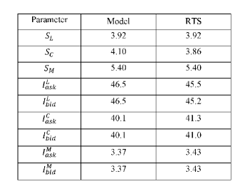
We define the parameter $I=179$ events/second. All other parameters in the balanced case are given in the table

Figure 16. Parameters in the balanced case.

The evolution of the price in our model is given below

Figure 17. Price in the balanced case.

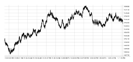
Apparently the price does not exhibit any preferred direction. We refer to [6] for details of this simulation.

5.3. The Disbalance of Liquidity in the Book.

By adjusting $s_{min}$ and $d_{min}$ one can model price movements. We assume that the all other rates on the sell and buy side are equal

$$I_{bid}^{M}=I_{ask}^{M},\qquad\qquad I_{bid}^{C}=I_{ask}^{C},\qquad\qquad I_{bid}^{L}=I_{ask}^{L}.$$

If $s_{min}>d_{min}$ then the book is thiner on the buy side (below the the price) and this leads to price decrease. If on the opposite $s_{min}<d_{min}$ then the book is thiner on the sell side (above the the price) and this leads to price increase.

Indeed, the dependence of $\delta_{sell}$ on the volume of sell market order $v_{M}$ is getting bigger as soon as $d_{min}$ is getting smaller. Similarly, dependence of $\delta_{buy}$ on the volume of buy market order $v_{M}$ is getting bigger as soon as $s_{min}$ is getting smaller. As a very crude approximation we can take

$$v_{M}\sim\delta_{sell}d_{min},$$

and

$$v_{M}\sim\delta_{buy}s_{min}.$$

Therefore,

$$\frac{\delta_{sell}}{\delta_{buy}}\sim\frac{s_{min}}{d_{min}}.$$

If $s_{min}<d_{min}$, then

$$\frac{\delta_{sell}}{\delta_{buy}}<1$$

and the price has to increase. If $s_{min}>d_{min}$, then

$$\frac{\delta_{sell}}{\delta_{buy}}>1$$

and the price has to decrease.

Figure 18. Thinning of the book on the buy or sell side.

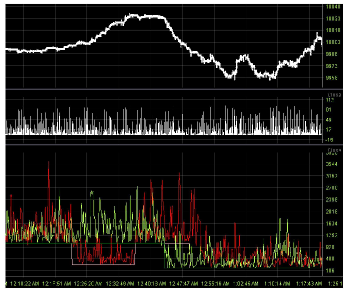
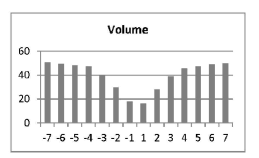
This is illustrated in Figure 18. The first graph is a price and the second graph which is the vertical column is the volume. The third graph is the graph for instantaneous liquidity $s$ and $d$. The white and green lines are the graphs $s_{min}$ and $d_{min}$. Depending on the relation between $s_{min}$ and $d_{min}$ one can observe increase or decrease of the price.

5.4. The Disbalance of Sell and Buy orders in the Order Flow.

Such disbalance occurs when $I_{bid}^{M}\neq I_{ask}^{M}.$ At the same time the condition $\Delta s=\Delta d=0$ holds. Figure 19 shows monotonous increase of the price. The first graph represent the price and the second two red and yellow lines are $s(5)$ and $d(5)$.

Figure 19. The upward trend.

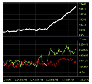
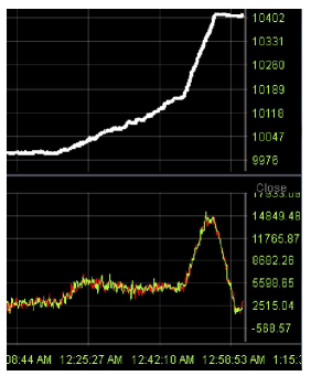
Figure 20 also shows monotonous increase of the price but instead of $s(5)$ and $d(5)$ it has graphs of $s$ and $d$.

Figure 20. The upward trend.

Kirill Vaninsky
Department of Mathematics
Michigan State University
East Lansing, MI 48824
USA
vaninsky@math.msu.edu

Alexander Glekin
Institute of System Analysis
RAN
Prospect 60 Oktyabria
Moscow 117312
Russia
AleksanderGlekin@gmail.com

Alexander Lykov
Faculty of Mathematics and Mechanics
Moscow State University
Vorobjevy Gory
Moscow
Russia
alexlyk314@gmail.com

References

- [1] Biais B., Hillion P., Spatt Ch. An Empirical Analysis of the Limit Order Book and the Order Flow in the Paris Bourse. Journ. of Finance, vol L, n. 5, pp. 1655–1689, 1995.
- [2] J.-P. Bouchaud, M. Mezard, and M. Potters. Statistical properties of the stock order books: empirical results and models. Quantitative Finance, 2(4), pp. 251–256, 2002.
- [3] A. Chakraborti, I.M. Toke, M. Patriarca, F. Abergel Econophysics review I. Empirical facts. Quantitative Finance, 2011,Vol. 11, No. 7, pp. 991–1012.
- [4] A. Chakraborti, I.M. Toke, M. Patriarca, F. Abergel Econophysics review II. Agent based models. Quantitative Finance, 2011,Vol. 11, No. 7, pp. 1013–1041.
- [5] D.K. Gode and S. Sunder. Allocative Efficiency of Markets with Zero-Intelligence Traders: Market as a Partial Substitute for Individual Rationality. The Journal of Political Economy, Vol. 101, No. 1. 1993, pp. 119-137
- [6] A.O. Glekin. Stochastic multi-agent model for the order book dynamics. The Program Products and Systems. vol. 3, 2013, pp. 283-288.
- [7] E. Samanidou, E. Zschischang, D. Stauffer and T. Lux (2007) Agent based models of financial markets. (2007) Rep. Prog. Phys. 70, pp. 409–450.
- [8] S. Muzychka, A. Lykov and K. Vaninsky (2012). A multi-agent nonlinear Markov model of the order book. arXiv:1208.3083 to appear.
- [9] S. Muzychka and K. Vaninsky. A class of nonlinear random walks related to the Ornstein-Uhlenbeck process. Markov Processes and Related Fields, (2012), vol.17, num. 2, pp. 277-304. arXiv:1107.0850.
- [10] E. Smith, J. D. Farmer, L. Gillemot, and S. Krishnamurthy. Statistical theory of the continuous double auction. Quantitative Finance, 3(6), pp. 481–514, 2003.
- [11] M. Daniels, J.D. Farmer, L. Gillemot, G. Iori, E. Smith. A quantitative model of trading and price formation in financial markets. Phys. Rev. Lett. 90, 108102, 2003.
- [12] S. Mike and J.D. Farmer. An Empirical Behavioral Model of Price Formation. Journal of economic dynamics and control. vol 32, 200, 2008.