The Luminosity Function at from 97 Y-band dropouts: Inferences About Reionization
Abstract
We present the largest search to date for Y-band dropout galaxies ( Lyman break galaxies, LBGs) based on 350 arcmin2 of HST observations in the V-, Y-, J- and H-bands from the Brightest of Reionizing Galaxies (BoRG) survey. In addition to previously published data, the BoRG13 dataset presented here includes approximately 50 arcmin2 of new data and deeper observations of two previous BoRG pointings, from which we present 9 new LBG candidates, bringing the total number of BoRG Y-band dropouts to 38 with (AB system). We introduce a new Bayesian formalism for estimating the galaxy luminosity function, which does not require binning (and thus smearing) of the data and includes a likelihood based on the formally correct binomial distribution as opposed to the often used approximate Poisson distribution. We demonstrate the utility of the new method on a sample of Y-band dropouts that combines the bright BoRG galaxies with the fainter sources published in Bouwens et al. (2011) from the Hubble Ultradeep Field (HUDF) and Early Release Science (ERS) programs. We show that the luminosity function is well described by a Schechter function over its full dynamic range with a characteristic magnitude , a faint-end slope of , and a number density of . Integrated down to this luminosity function yields a luminosity density, . Our luminosity function analysis is consistent with previously published determinations within 1. The error analysis suggests that uncertainties on the faint-end slope are still too large to draw firm conclusion about its evolution with redshift. We use our statistical framework to discuss the implication of our study for the physics of reionization. By assuming theoretically motivated priors on the clumping factor and the photon escape fraction we show that the UV luminosity density from galaxy samples down to can ionize only 10-50% of the neutral hydrogen at . Full reionization would require extending the luminosity function down to . The data are consistent with a substantial fraction of neutral hydrogen at , in agreement with recent suggestions based on deep spectroscopy of redshift 8 LBGs.
Subject headings:
cosmology: observations — galaxies: evolution — galaxies: formation — galaxies: high-redshift1. Introduction
Characterizing the epoch of reionization, i.e., the epoch at which the first stars and galaxies in the Universe reionized the vast majority of the neutral hydrogen, is a key outstanding issue in the continued effort to map the formation and early evolution of galaxies. For almost four years, since the installment of the Wide Field Camera 3 (WFC3) onboard the Hubble Space Telescope (HST), the frontier of this knowledge has been pushed further and further back towards the dawn of cosmic reionization.
At present, several hundred high redshift galaxy candidates have been found at redshift (e.g., Stark et al., 2010; Bouwens et al., 2007, 2012; Ouchi et al., 2010; Bradley et al., 2013), and with the improved near-IR efficiency of WFC3 the search for candidates has been pushed to using the Lyman Break technique. In particular the Hubble Ultra Deep field efforts in 2009 (Oesch et al., 2010b, c; Lorenzoni et al., 2011; Bouwens et al., 2010, 2011; McLure et al., 2010) and 2012 (Koekemoer et al., 2012; Ellis et al., 2012; Dunlop et al., 2012b; Schenker et al., 2013; McLure et al., 2013; Ono et al., 2012a; Oesch et al., 2013; Illingworth et al., 2013) have revealed the faintest samples of galaxy candidates at . Simultaneously larger area observations are targeting brighter and rarer candidates, either in legacy fields, such as GOODS/CANDELS (Grogin et al., 2011; Koekemoer et al., 2011), or in pure-parallel random pointings, like those of our Brightest of Reionizing Galaxies Survey111https://wolf359.colorado.edu (hereafter BoRG, Trenti et al., 2011, 2012b; Bradley et al., 2012).
Our ongoing BoRG survey has two key goals. The first goal is to provide bright targets that can potentially yield spectroscopic confirmation of galaxies by follow-up observations (Treu et al., 2012, 2013). In fact, while dropout samples have extensive spectroscopic redshifts, (e.g., Vanzella et al., 2009; Stark et al., 2010, 2013), only a handful of galaxies (e.g., Ono et al., 2012b) have currently confirmed redshifts with the highest being at (Finkelstein et al., 2013). So far no Y-band dropout at has been spectroscopically confirmed. Only upper limits on Ly flux have been provided to date (Caruana et al., 2012, 2013; Capak et al., 2013; Treu et al., 2013; Faisst et al., 2014) and those leave open the interpretation of whether the photometric selection technique breaks down at (which would be surprising given the small change in magnitudes and filters) versus the more interesting physical explanation of an increase in the intergalactic medium (IGM) optical depth to Ly arising from a higher neutral hydrogen fraction at (Treu et al., 2013) with respect to redshift 7 (Fontana et al., 2010) and 6 (Stark et al., 2010, 2013).
The second goal of the BoRG survey is to improve the determination of the luminosity function, by identifying rare and bright dropouts to extend the dynamic range of observations in smaller area deep fields, which are dominated by fainter sources. An accurate measure of the luminosity function is necessary not only to study how galaxies evolve across time, but also to quantify the photon budget available for hydrogen ionization (Trenti et al., 2010; Zaroubi, 2013; Dunlop, 2013). At lower redshift, it is well established (Bouwens et al., 2007) that the luminosity function is accurately described by a Schechter function (Schechter, 1976) so it is natural to expect a similar form at higher redshift. However, data covering a wide dynamic range are needed to establish that this is indeed the case, and to resolve the degeneracy between the Schechter function parameters in the luminosity function fit (Bradley et al., 2012; Oesch et al., 2012).
In this paper we have two goals. The first is to present the complete sample of Y-band dropouts from the BoRG cycle-19 data, and to use these in combination with the literature to determine the galaxy luminosity function at . The second goal is to study the consequences for cosmic reionization the inferred luminosity function has. To determine the luminosity function we develop and implement a rigorous statistical Bayesian method to infer the posterior distribution function of the parameters of the luminosity function from the data. The method supersedes those commonly adopted in this field (e.g Bradley et al., 2012; McLure et al., 2013; Schenker et al., 2013; Oesch et al., 2012) in several ways: the data are not binned, thus avoiding smearing the luminosity function (Trenti & Stiavelli, 2008); the flux uncertainties are correctly taken into account; the counts are modeled using the formally correct binomial distribution (Kelly et al., 2008), instead of the Poisson approximation; the full posterior probability distribution function is computed using Markov Chain Monte Carlo methods instead of relying on maximum likelihood estimators based on the asymptotic covariance matrix from the observed Fisher information for uncertainties. By applying this framework to a large sample of galaxies, consisting of objects both bright (from BoRG) and faint (from the Hubble UDF/ERS fields), we show that the credible intervals include previous best-fit estimates By treating the problem in a self-consistent statistical manner we carry out an inference about reionization by combining the inferred observational uncertainties with various theoretical priors.
The paper is organized as follows. We start by briefly describing the BoRG survey in Section 2. The current sample of Y-band dropouts containing 9 new and 2 improved galaxy candidates (BoRG13) with respect to those previously published by our team (BoRG09; BoRG12 Trenti et al., 2011; Bradley et al., 2012) is described in Section 3. Two Appendixes (A and B) take advantage of the follow-up observations of one field and of the large number of BoRG pointings to characterize and discuss the statistics of detections and contaminants in dropout searches. In Section 4 we apply our inference of the Schechter luminosity function parameters using our rigorous Bayesian framework, discussed in detail in Appendix C. The results are presented and discussed in the context of cosmic reionization in Section 5. A brief summary is given in Section 6.
All magnitudes are AB magnitudes and a standard concordance cosmology with , , and is assumed.
2. The BoRG Survey
The galaxy candidates from the latest data obtained as part of the BoRG survey are described briefly below. We refer the reader to Trenti et al. (2011) and Bradley et al. (2012) for a more in-depth description of the survey.
The BoRG survey is a pure-parallel WFC3 imaging HST program. As of April 2013 the survey has obtained 350 arcmin2 of visual and near-infrared HST photometry over 71 fields randomly located in the sky. The pure-parallel nature of the survey implies that the survey area is divided into 71 independent lines of sight on the sky, reducing sample (or cosmic) variance below the level of statistical noise (Trenti & Stiavelli, 2008; Bradley et al., 2012). 53 out of the 71 fields represent the core of the BoRG survey and have been observed in the four WFC3/HST filters F606W, F098M, F125W, and F160W. This was primarily done as part of programs GO/PAR 11700 and GO/PAR 12572 (PI: Trenti) complemented by a small number of COS-GTO coordinated parallels. One of these 53 fields furthermore has data in F105W from a recent follow-up campaign (described in Appendix A). The core of BoRG is complemented by other archival data consisting of 8 fields from GO/PAR 11702 (PI: Yan, Yan et al., 2011) and 10 COS-GTO fields, where instead of the F606W-band the F600LP-band was used. For a discussion of the benefits of using F606W, as in the BoRG core, instead of F600LP see Bradley et al. (2012).
In this work we will refer to F606W, F098M, F125W, and F160W as V-, Y-, J-, and H-band observations unless mentioned otherwise. Note that the data added in BoRG13 only has F606W V-band observations as opposed to BoRG09 and BoRG12 which also contained F600LP V-band data.
3. Y-band dropout sample
The dropout technique (Steidel et al., 1996, 2000; Madau et al., 1996) was applied to the BoRG data to identify galaxy candidates as detailed in Section 3.2
The first fields of the BoRG survey (referred to as BoRG09 and BoRG12) were analyzed by Trenti et al. (2011, 29 fields) and Bradley et al. (2012, 29+30=59). Based on this data, Bradley et al. (2012) presented a sample of 33 Lyman break galaxy (LBG) candidates at and estimated the corresponding high-redshift luminosity function.
In this work we augment this sample by analyzing 13 additional fields, taken in HST Cycle 19 (GO/PAR 12572, PI: Trenti). Note that the field BoRG_1510+1115 also appeared in the study by Bradley et al. (2012) based on partial data. This field is therefore included in the present analysis and supersedes the previous release. Results of the analysis of the 13 new fields are presented in the next Section 3.1. We also present an updated analysis of BoRG_1437+5043 based on deeper and wider-field observations obtained in November 2012 (GO 12905, PI: Trenti). We describe these observations in Appendix A.
3.1. The Latest Survey Extension: BoRG13
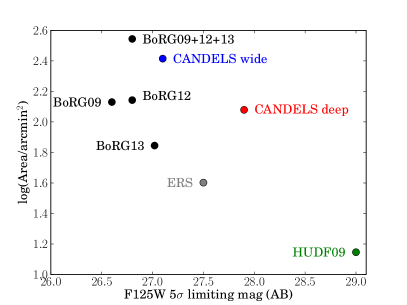
The 13 new Cycle 19 BoRG fields are summarized in Table 1 together with the follow-up in BoRG_1437+5043. Together with Table 1 and Table 2 of Bradley et al. (2012) this summarizes the current status of BoRG09, BoRG12, and BoRG13. This brings the total J-band area of the BoRG survey to 350 arcmin2. This makes BoRG the largest existing area which can be searched for Y-band dropouts. In comparison, the CANDELS (Koekemoer et al., 2011; Grogin et al., 2011) survey has Y-band coverage of approximately 260 arcmin2 (wide) and 120 arcmin2 (deep). Furthermore the depth reached by BoRG (J and H ) at has not been achieved from the ground over large areas. The depth and area of the BoRG campaigns are compared with those achieved by other surveys in Figure 1.
As noted in above and shown in Bradley et al. (2012) the effect of large scale structures, i.e. cosmic variance, is less important than the statistical noise for the BoRG12 sample. Extending BoRG12 by the 13 new randomly pointed fields of BoRG13 makes cosmic variance even more negligible.
The BoRG13 fields were reduced using publicly available code. First,
the cosmic rays were removed in each exposure using the Laplacian
cosmic ray detection developed by van Dokkum (2001).
The individual exposures in each filter were then combined using
AstroDrizzle (the replacement of MultiDrizzle as of June 2012 Koekemoer et al., 2003).
The images were drizzled to a final pixel scale of /pixel
using a ‘pixfrac’ of 0.75 as in our previous analyses.
The correlated noise introduced by this drizzling (e.g., Casertano et al., 2000)
is explicitly corrected for by normalizing the r.m.s. maps by the
empirical noise as described by Trenti et al. (2011).
The 5 limiting magnitudes () and exposure times
obtained in each field are quoted in Table 1.
Having created the reduced science images and r.m.s. maps we used
SExtractor (Bertin & Arnouts, 1996) in dual-image mode with
the J-band image as detection image to create source catalogs in each of
the available photometric bands. These catalogs where used to search
for Y-band dropouts as described in Section 3.2. In this
process signal-to-noise (S/N) was estimated using isophotal apertures
(ISOMAG) whereas total magnitudes are estimated in scalable
Kron apertures (AUTOMAG).
This approach follows the well-established procedure adopted and described by Bradley et al. (2012), and we refer to this work for further details.
| Field | F606W | F098M | F105W | F125W | F160W | Area | E(BV) | |||||||
| [deg] | [deg] | [s] | [s] | [s] | [s] | [s] | [′2] | |||||||
| BoRG_0456-2203 | 73.9646 | -22.0489 | 2647 | 26.58 | 3718 | 26.75 | 1809 | 26.74 | 1809 | 26.52 | 3.06 | 0.038 | ||
| BoRG_0951+3304 | 147.7003 | 33.0737 | 2660 | 26.43 | 4518 | 26.43 | 2212 | 26.52 | 2212 | 26.20 | 1.82 | 0.013 | ||
| BoRG_0952+5304 | 147.9448 | 53.0714 | 2506 | 26.78 | 3912 | 26.69 | 1806 | 26.77 | 1806 | 26.50 | 3.72 | 0.011 | ||
| BoRG_1059+0519 | 164.7039 | 5.3125 | 2386 | 26.43 | 3812 | 26.72 | 1806 | 26.83 | 1806 | 26.38 | 2.15 | 0.028 | ||
| BoRG_1118-1858 | 169.4101 | -18.9726 | 8514 | 26.94 | 13235 | 27.13 | 6276 | 27.17 | 6276 | 26.94 | 2.04 | 0.050 | ||
| BoRG_1358+4326 | 209.4754 | 43.4338 | 2451 | 26.77 | 3812 | 26.77 | 1606 | 26.83 | 1606 | 26.47 | 3.86 | 0.008 | ||
| BoRG_1358+4334 | 209.4636 | 43.5610 | 4866 | 27.02 | 7023 | 27.21 | 3812 | 27.32 | 3812 | 27.06 | 2.71 | 0.007 | ||
| BoRG_1416+1638 | 214.0048 | 16.6269 | 3112 | 26.86 | 5271 | 26.84 | 2462 | 26.85 | 2462 | 26.55 | 3.64 | 0.020 | ||
| BoRG_1429-0331 | 217.3717 | -3.5185 | 9164 | 26.96 | 13235 | 27.06 | 5726 | 27.00 | 5726 | 26.79 | 3.37 | 0.083 | ||
| BoRG_1437+5043_r1 | 219.2153 | 50.7244 | 13570 | 27.15 | 19720 | 26.98 | 11394 | 27.04 | 10691 | 26.66 | 1.66 | 0.013 | ||
| BoRG_1437+5043_r2b | 219.2153 | 50.7244 | 13570 | 27.70 | 19720 | 27.65 | 8885 | 27.21 | 11394 | 27.74 | 10691 | 27.49 | 1.67 | 0.013 |
| BoRG_1437+5043_r3b | 219.2153 | 50.7244 | 13570 | 27.54 | 19720 | 27.42 | 8885 | 27.14 | 11394 | 27.54 | 10691 | 27.39 | 1.52 | 0.013 |
| BoRG_1459+7146 | 224.7501 | 71.7638 | 3724 | 26.61 | 6023 | 26.75 | 2812 | 27.04 | 2812 | 26.82 | 2.78 | 0.027 | ||
| BoRG_1510+1115 | 227.5371 | 11.2415 | 13315 | 27.19 | 21059 | 27.43 | 9529 | 27.67 | 9529 | 27.16 | 1.78 | 0.046 | ||
| BoRG_2132-1202 | 322.9467 | -12.0397 | 2656 | 26.20 | 3718 | 26.19 | 1809 | 26.23 | 1809 | 26.00 | 1.21 | 0.062 | ||
| BoRG_2313-2243 | 348.2326 | -22.7252 | 8308 | 26.98 | 13335 | 27.11 | 6326 | 27.11 | 6326 | 26.91 | 3.26 | 0.026 | ||
| Note. – a5 magnitude limits are for apertures corrected for Galactic extinction. The total effective search area for Y-band | ||||||||||||||
| dropouts in BoRG13 is 40.26 arcmin2. The combined effective search area for Y-band dropouts in BoRG09 + BoRG12 + BoRG13 is | ||||||||||||||
| 247 arcmin2. bInclude follow-up observations from November 2012 (GO 12905, PI: Trenti) described in Appendix A. | ||||||||||||||
3.2. Selecting Galaxy Candidates in BoRG13
The selection of the high redshift LBGs closely follows Trenti et al. (2011) and Bradley et al. (2012). We use an identical Y-band dropout selection scheme, i.e., we require that
| (1) | |||||
| (2) | |||||
| (3) | |||||
| (4) | |||||
| (5) |
in each of the fields from Table 1. The colors are insensitive to whether isophotal, Kron or aperture magnitudes are used (Finkelstein et al., 2010; Trenti et al., 2012b). Candidates passing these selection criteria have been vetted by visual inspection to remove false positives such as hot pixels and diffraction spike features from bright objects.
As in our previous work, the SExtractor stellarity index was used as
an additional criterion to help reject stars as potential
contaminants. For the J-band 8 sources the stellarity index is quite
reliable and we required it to be .
For sources with ,
the stellarity index is more noisy and therefore we
did not imply a strict cut, but we used it as a criterion in
combination with visual inspection. Three of the authors (KBS, TT, MT)
inspected all the dropouts independently with the aim of rejecting
spurious or star-like features. After the initial independent
classification each dropout was discussed by the three co-authors
resulting in the consensus list given in this paper.
Only a few objects did not initially get rejected by all authors. These were potential hot
pixels being mistaken for real sources in the drizzled un-dithered BoRG data and potential
stars (point-like sources).
In the former case disagreement led to exclusion from the final sample whereas objects were
revisited to obtain agreement in the latter case.
We note that the final list therefore includes potential real-source contaminants.
However, invoking a relatively high fiducial contamination fraction of the
dropout sample as described in Section 4.2 this is
accounted for when inferring the intrinsic luminosity function.
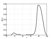
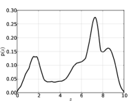
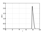
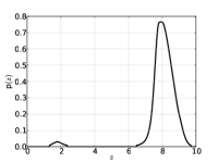
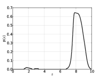
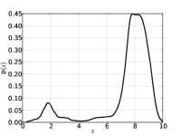
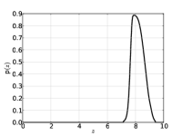
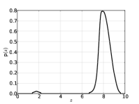
The new dataset includes 11 sources passing our selection criteria. 9 of these are new findings, while two (BoRG_1437+5043_r2_637 and BoRG_1510+1115_1218) are candidates initially presented by Trenti et al. (2011) and Bradley et al. (2012) and are now confirmed at higher S/N by the deeper data. The sample of BoRG13 galaxy candidates is summarized in Table 2. In Figures 2 and 3 we show 3′′x3′′ postage stamps of all 11 BoRG13 redshift 8 galaxy candidates.

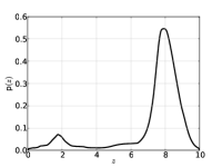

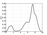

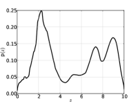








Combining the BoRG13 sample with the updated samples from BoRG09 and BoRG12 results in a total sample of 38 bright galaxy candidates at from the BoRG survey. Note that a ‘’ detection in this context means . As we discuss in Appendix B, the noise background distribution is highly non-Gaussian with significant broader wings. As discussed in the appendix, our requirement of two-band detections and non-detections at bluer bands, is essential to avoid contaminants, especially in the 5 sample. 10 of the 38 candidates have .
| ID | J | Y J | J H | S/N | S/N | S/N | S/N | ||
| BoRG_0456-2203_904 | 73.97655 | -22.04115 | 26.72 0.27 | 2.1 0.9 | -0.2 0.4 | 0.8 | 0.8 | 5.1 | 3.5 |
| BoRG_0951+3304_277a | 147.68443 | 33.07019 | 25.87 0.22 | 2.3 0.7 | -0.2 0.3 | -0.6 | 1.2 | 7.9 | 5.3 |
| BoRG_1059+0519_991 | 164.69864 | 5.32262 | 26.34 0.31 | 1.8 0.6 | -0.2 0.4 | 0.7 | 1.6 | 5.9 | 3.6 |
| BoRG_1358+4334_482 | 209.44475 | 43.55779 | 26.91 0.26 | 2.0 0.8 | 0.0 0.3 | 1.3 | 0.4 | 6.4 | 4.9 |
| BoRG_1437+5043_r2_637a,b | 219.21058 | 50.72601 | 25.76 0.07 | 3.2 0.8 | 0.1 0.1 | -0.2 | 1.0 | 20.2 | 16.5 |
| BoRG_1510+1115_354a | 227.54706 | 11.23145 | 27.03 0.22 | 2.1 0.7 | -0.1 0.3 | 0.1 | 1.2 | 7.7 | 4.6 |
| BoRG_1510+1115_1218a,c | 227.54266 | 11.26152 | 26.87 0.22 | 2.2 0.8 | 0.0 0.3 | 0.8 | 0.7 | 7.3 | 5.2 |
| BoRG_1510+1115_1487a | 227.53173 | 11.25254 | 27.60 0.24 | 2.0 0.8 | 0.0 0.4 | 0.4 | 0.5 | 5.8 | 4.0 |
| BoRG_1510+1115_1524a | 227.53812 | 11.25552 | 26.63 0.15 | 2.3 0.6 | 0.0 0.2 | -0.8 | 1.5 | 11.9 | 7.9 |
| BoRG_1510+1115_1705a | 227.54008 | 11.25111 | 27.00 0.19 | 1.8 0.6 | -0.8 0.4 | -2.0 | 1.6 | 8.4 | 2.6 |
| BoRG_2313-2243_1136 | 348.24871 | -22.71342 | 27.14 0.26 | 2.3 0.8 | -0.1 0.3 | -0.3 | 1.0 | 6.4 | 4.8 |
| Note. – J-band magnitudes are corrected for galactic extinction using the Cardelli et al. (1989) extinction law and the | |||||||||
| E(BV) from Table 1. aFollowed up with MOSFIRE as presented in Treu et al. (2013). bPresented in Trenti et al. (2011) | |||||||||
| and Bradley et al. (2012) as BoRG58_1787-1420 and BoRG_1437+5043_1137, respectively. For previous photometry | |||||||||
| of this candidate see the ‘B1437_r2_0637_T12a’ rows in Table 5. cPresented in Bradley et al. (2012) as | |||||||||
| BoRG_1510+1115_1404. The HST postage stamps and the photometric redshift probability distribution for each | |||||||||
| candidate are shown in Figures 2 and 3. | |||||||||
3.3. Photometric Redshifts
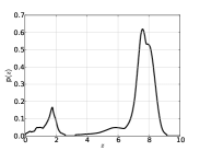
The Bayesian photometric redshift code BPZ (Benítez et al., 2004; Coe et al., 2006) was run on the photometry for each of the LBG candidates shown in Table 2 providing photometric redshift probability distributions, , for each individual object. In Figures 2 and 3 we show the obtained using a flat prior on the redshift distribution. In all cases prominent probability peaks are seen at the expected Y-band dropout redshift of 7.4–8.8.
4. Estimating the Luminosity Function
In this section we present the Bayesian framework applied to infer the luminosity function parameters. We use the empirical Schechter function (Schechter, 1976),
| (6) |
(see also Appendix C), as our luminosity function model. Hence, the luminosity function parameters to fit are the faint-end slope, , the ‘knee’, , characterizing the transition between the power-law part at the faint end and the exponential cut-off at the bright end of the distribution, and the normalization . As described by, e.g., Bradley et al. (2012) and Oesch et al. (2012) and are degenerate. This implies that both bright objects (the latter, for instance in case of the BoRG sample) and faint objects are needed to obtain precise estimates of both and . We will illustrate this degeneracy in Section 5 by applying our framework to a sample of faint LBGs only. The normalization represents the co-moving number density of objects described by the luminosity function. The density is directly related to the total number of high-redshift objects, , in the surveyed volume, , as described below (Equation (9) and Appendix C).
The framework used to fit the Schechter function in the present study improves on the standard formalism typically adopted to estimate luminosity functions in the literature. In particular we improve on three main issues with luminosity function fitting that seems to have become standard practice in the high redshift community
First of all it is often assumed that the likelihood follows a Poisson distribution (e.g., Bradley et al., 2012; Schenker et al., 2013; McLure et al., 2013; Oesch et al., 2012). As described by Kelly et al. (2008), the Poisson distribution is only an approximation of the formally correct binomial distribution. To the extent that the detection probability is small and the total number of objects in the parent sample is large, the binomial distribution reduces to the Poisson distribution. Hence, in the case of rare-object luminosity functions the Poisson distribution is a fair approximation. Effects like cosmic variance (Schenker et al., 2013) will further smear and reduce any significant differences and we therefore do not expect any strong bias in the shape of the luminosity function from this approximation. Nevertheless it is important to quantify this statement, by applying the formally correct binomial distribution, and verify that this is indeed not the case.
Secondly, it has become generally accepted to use binned samples of dropouts when estimating the luminosity functions (e.g., Bouwens et al., 2006, 2007, 2011; Bradley et al., 2012; McLure et al., 2013; Schenker et al., 2013) instead of using the actual data themselves. Such an approach intentionally reduces the information to an arbitrarily defined set of bins which is sub-optimal and introduces smoothing on the scale of the bins thus potentially biasing the inference to flatter distributions (Cara & Lister, 2008; Yuan & Wang, 2013).
Lastly, the photometric errors on the individual sources in the high-redshift samples are often not modeled directly when obtaining the luminosity function parameters. Bouwens et al. (2007, 2011) use a set of generalized transfer functions to model the effect of photometric scatter in their samples and simulations similar to the ones described in Section 4.1 are used to account for photometric scatter in and out of the color selection boxes (Bradley et al., 2012; Oesch et al., 2012), or between adjacent bins in the binned luminosity function (Schenker et al., 2013). However, due to the binning of the data when fitting the luminosity function this does not fully account for the photometric uncertainty of the individual objects in the sample. Certainly previous approaches provided an approximate treatment, but direct modeling of the photometric uncertainties themselves makes full use of all the available information and provides more rigorous results.
The formalism applied in this study is therefore drawing from a posterior distribution using a likelihood based on the binomial distribution described by Kelly et al. (2008), avoiding binning of the data completely and thereby estimating the luminosity function using the full information directly, and lastly, explicitly modeling the photometric error distribution of the sample by assuming the errors are Gaussian distributed.
The posterior distribution for Y-band dropouts can be summarized as (see Appendix C)
| (7) | |||||
Here where and are the main Schechter luminosity function parameters and is the number of high- LBGs in the surveyed co-moving cosmological volume, which as mentioned is closely related to , the Schechter function normalization. is the set of observed J-band luminosities and indicates that the object is a V-band non-detection as required by the dropout selection described in Section 3.2. On the right-hand-side represents the prior assumptions on the problem and the factors are binomial coefficients. We assume uniform priors on , and . is the probability distribution of an object making it into the dropout sample which is independent of the individual objects in the sample, and is the likelihood function for the observed J-band luminosity of the ’th object in the sample. is the area of the individual fields in the BoRG13 sample, which each contain high redshift candidates () and have an assumed contamination of . is the area of the full sky. In Appendix C we give the expanded expression of the posterior distribution from Equation (7) which was actually used when performing the luminosity function parameter inference. We note that in the current framework the prior on the redshift of the individual LBG candidates is not explicitly taken into account. We refer to Appendix C for further details.
A posterior distribution function as the one shown in
Equation (7) is well suited for Markov Chain Monte Carlo (MCMC)
sampling over the luminosity function parameters .
Calculating the posterior probability enables a
robust determination of the luminosity function as preferred by the
data given the sample of sources. We used the Python pymc
package222Available at http://pymc-devs.github.io/pymc/ with a
Robust Adaptive Metropolis (RAM; Vihola, 2012) algorithm to sample
the luminosity function parameters , , and .
The RAM algorithm adapts the proposal covariance matrix to obtain a fixed acceptance ratio
(set to 0.4 in this work).
4.1. Selection and Completeness Functions
When estimating the luminosity function a crucial part of the expression for the posterior distribution is the selection function including an estimate of the completeness of the source selection. Here we have used two distinct selection functions.
For each of the BoRG fields we explicitly split the total selection function into a completeness function and a selection function not including completeness . and were simulated as described by Oesch et al. (2007, 2009, 2012) and Bradley et al. (2012). In summary, the steps in obtaining these functions are:
-
•
Sources with different spectral energy distribution, luminosity, redshift, and size are added to the original science images. The simulated galaxies are galaxies rescaled to higher redshift using a size relation of as determined from LBG samples (Bouwens et al., 2004; Ferguson et al., 2004; Oesch et al., 2010a) and their UV-continuum slopes (Dunlop et al., 2012a; Finkelstein et al., 2012; Bouwens et al., 2012).
-
•
The detection and selection procedure described in Section 3 is re-run for each field to determine and .
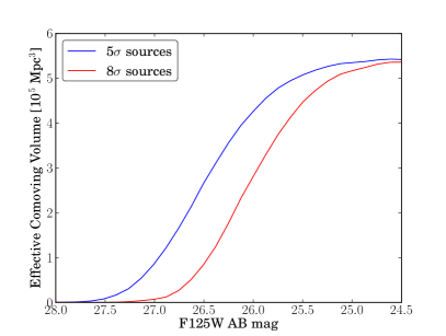
The selection function (used in Section C.2) is as mentioned corrected for completeness. When estimating the intrinsic luminosity function the BoRG13 LBGs are all assumed to be at . Hence, when sampling the posterior for the BoRG fields
| (8) |
The effective volume of the BoRG survey is derived from the full selection function as a function of J-band magnitude, i.e., . The total effective co-moving volumes for the 5 and 8 BoRG13 samples are shown in Figure 4
To break the - parameter degeneracy we used a sample of 59 faint LBGs from the Hubble Ultradeep Field (HUDF) and Early Release Science (ERS) programs (Tables 14–17 in Bouwens et al., 2011) to populate the faint end of the distribution when fitting the luminosity function. For this sample a piecewise selection function following the binned data presented in Bouwens et al. (2011) was used. Integration over this selection function was done using linear interpolation between the bins. Note that the effect of large-scale structures (cosmic variance) on the luminosity functions in the HUDF/ERS luminosity range is very modest as described by Bouwens et al. (2011).
Both the BoRG and HUDF/ERS selection function models are explicitly set to 1 and 0 for luminosities brighter than and fainter than the modeled luminosities, respectively.
4.2. Contamination
When estimating the number of contaminants among the BoRG LBG candidates we follow the approach taken by Bradley et al. (2012). We use a fiducial average contamination level of for the BoRG sample. (In Section 5.1 we investigate the effects of modifying this assumption on the shape of the luminosity function) The contamination of the HUDF/ERS sample is included in the selection function described above and is therefore assumed to be 0.0 for the Bouwens et al. (2011) sample. The available information about the contaminants at redshift 8 is limited and distinguishing between the luminosity function of the contaminants and the LBGs complicates matters considerably Hence, we assume that the fraction of contaminants is independent of luminosity for the BoRG sample. In Equation (7) The number of contaminants are approximated by their expectation values as explained in Appendix C.
Having obtained and assuming that the luminosity function does not evolve over the redshift interval of interest, the number density is obtained by calculating (see Equation (C4) in Appendix C)
| (9) |
Here is the co-moving cosmological volume of the ideal full-sky survey. To avoid divergence of the integral we set our lower integration limit of the luminosity function to erg/s which corresponds to an absolute magnitude of . Hence, sets the lower bound for what we include as “a galaxy” in our analysis. With an estimated normalization of the sample luminosity function, the luminosity density, , is obtained by integrating the luminosity function multiplied by the luminosity itself (see Appendix C).
4.3. Sanity Check of Bayesian Framework
Prior to applying the newly developed Bayesian inference framework to the BoRG13 data it was tested extensively on a set of simulated data samples. We confirmed that in all cases the MCMC sampling recovered the input luminosity functions from which the emulated samples were drawn. We also tested the code on the LBG sample analyzed in Bradley et al. (2012) (BoRG12). The obtained luminosity function had a faint-end slope of and in agreement with the and presented by Bradley et al. (2012). Within the 1 confidence intervals these measurements of both and are fully consistent. We note that we do not expect the results to be identical, since our framework avoids some of the approximations of previous studies.
5. Results
From the framework described in Section 4 the assumed intrinsic luminosity function for a sample of objects can be determined. In the following we will describe and summarize our findings from applying our framework to the 97 LBG candidates from the combined samples of BoRG13 and HUDF/ERS from Bouwens et al. (2011). We note that to ease comparison with the literature we convert into in the remainder of this work using that with .
| Reference | [Mpc-3] | [erg/s/Hz/Mpc3] | ||
|---|---|---|---|---|
| BoRG13 sample (This work) | ||||
| BoRG13 sample (This work) | ||||
| Bradley et al. (2012) | ||||
| Oesch et al. (2012) | ||||
| Bouwens et al. (2011) | ||||
| Lorenzoni et al. (2011) | (fixed) | |||
| Trenti et al. (2011) | (fixed) | (fixed) | ||
| McLure et al. (2010) | (fixed) | (fixed) | ||
| Bouwens et al. (2010) | (fixed) | (fixed) | ||
| Schenker et al. (2013) | ||||
| McLure et al. (2013) | (but see their Figure 7) | |||
| Note. – Estimated from the luminosity function parameters via the method described in Appendix C integrated | ||||
| down to at Å using . A small 0.13dex offset between these estimates and the | ||||
| literature was found. This difference can be recovered using suggesting that a value similar to this | ||||
| was used in, e.g., Oesch et al. (2012); Bouwens et al. (2011) and McLure et al. (2013). From Oesch et al. (2012) and | ||||
| Bouwens et al. (2011), respectively, where the luminosity function was integrated down to for Å. | ||||
| From Lorenzoni et al. (2011) where the luminosity function was integrated down to for Å. | ||||
| From Bouwens et al. (2010) where the luminosity function was integrated down to for Å. | ||||
5.1. The Luminosity Function at from BoRG13
We apply the inference framework to the full BoRG13 sample of 38 objects augmented by the fainter 59 candidates presented in Bouwens et al. (2011). For a consistency check on a more robust determination of the luminosity function bright end, we also consider a restricted BoRG13 sample consisting of the 10 objects in BoRG13 detected at , similarly to the approach followed by Bradley et al. (2012). This additional step allows us to validate the luminosity function derived from the full sample, which might be affected by photometric scatter as discussed in Appendices A and B.
When sampling the posterior distribution (given in Appendix C Equation (C15)) we use the selection functions described in Section 4.1, i.e., interpolation over a piecewise selection function for the HUDF/ERS data from Bouwens et al. (2011) and the simulated selection and completeness functions for the 5 and 8 BoRG samples at .
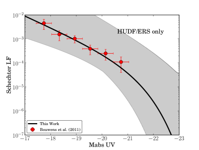
The results from sampling after an MCMC burn-in phase are shown in Figure 5. From top to bottom we show the results from fitting the Schechter luminosity function to the BoRG13 5, BoRG13 8 (both including the Bouwens et al. (2011) sample), and the Bouwens et al. (2011) samples. The latter is presented to illustrate the prominent degeneracy between the and luminosity function parameters without the bright BoRG LBGs to constrain the bright end of the distribution and break the degeneracy. The 1 and 2 confidence intervals are indicated by the red contours.
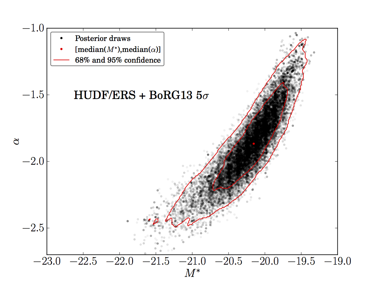
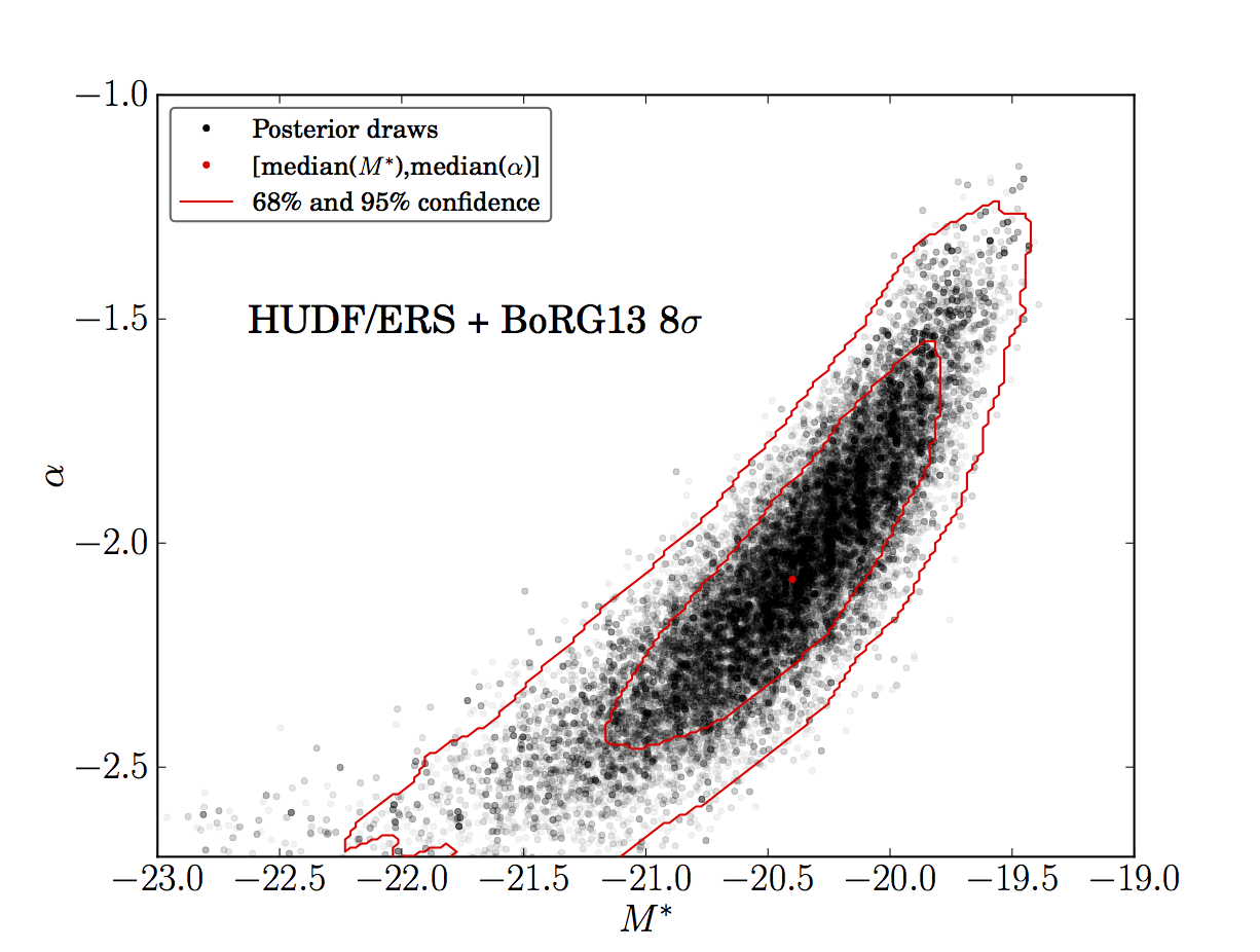

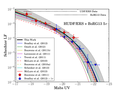
In Table 3 the results from the full BoRG13 luminosity function and the BoRG13 luminosity function only using the 8 candidates are summarized together with a selection of recent luminosity function fits from the literature. The BoRG13 luminosity function parameters and agree well with the literature values, confirming that the Poisson approximation is indeed a fair approximation when fitting luminosity functions at , in terms of best-fit value. We note that the BoRG13 5 best-fit faint-end slope is fully consistent within the 1- error bars with the literature values. We also note that the BoRG13 5 faint-end slope of -1.87 is fully consistent with the faint-end slope obtained from the BoRG12 data using the framework presented here () within the 1 error bars and fall comfortably within the 68% confidence interval contour when also considering the degeneracy with in the top panel of Figure 5.
The luminosity functions corresponding to each of the MCMC samples shown in Figure 5 are compared to the literature luminosity functions from Table 3 in Figure 6.
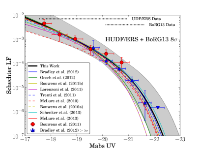
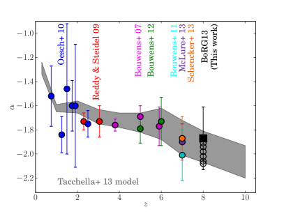
The relatively shallow best-fit faint-end slope of -1.87 for the BoRG13 5 sample might question the speculated steepening of the luminosity function at . Such a steepening is expected from galaxy formation models and cosmological simulations (Trenti et al., 2010; Jaacks et al., 2013; Tacchella et al., 2013), and would be related to the evolution of the slope of the dark matter halo mass function at the scale of which is characteristic for hosting the faint galaxies observed in the HUDF. To place our latest determination of in the broader context of other studies, Figure 7 shows the redshift evolution predicted by a recent theoretical models (e.g., Tacchella et al., 2013; Cai et al., 2014), together with estimated UV luminosity function faint-end slopes at (Oesch et al., 2010a), (Reddy & Steidel, 2009), (Bouwens et al., 2007), (Bouwens et al., 2012), and (Bouwens et al., 2011). As the error bars on our -estimate are still fairly large with a potential decline is still very possible within 1. Even though cosmic variance is insignificant over the full BoRG13 sample, it is important to check that it does not have a significant effect on the estimate of the faint-end slope, which is based on only three quasi-independent fields (HUDF). Based on the calculations by Trenti & Stiavelli (2008), the additional uncertainty due to cosmic variance is , which is small compared to the statistical uncertainty of our study, and therefore can be neglected.
This all highlights that significantly larger samples of faint as well as bright redshift 8 galaxies are needed to robustly determine the luminosity function shape and to confirm the suggested steepening of with redshift. We note that the more robust BoRG13 8 sample has a steeper faint-end slope and therefore favors a steepening of despite the marginally larger error bars compared to the BoRG13 5 sample.
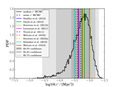
From the MCMC samples of we estimate the number density of high redshift objects, , and the luminosity density, , using the expressions given in Section 4.2 and Appendix C. The distributions of the obtained and values for the BoRG13 5 and 8 samples are shown in Figure 8. The median estimates and their uncertainties are quoted in Table 3. The values were obtained by integrating down to the HUDF magnitude limit of (Bouwens et al., 2011). Integrating to fainter magnitudes, i.e., extrapolating outside the data range, increases the luminosity density itself as well as the uncertainties.
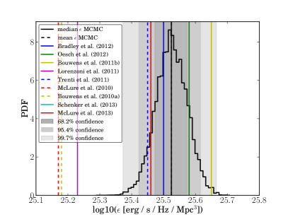
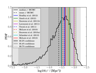
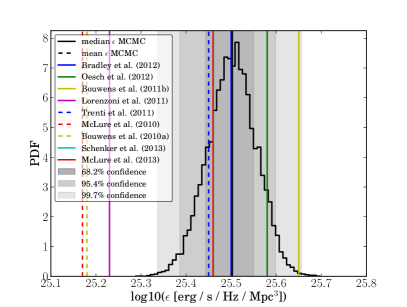
In Figure 9 we present the full multi-dimensional parameter space , , , and for the BoRG13 MCMC inference (the lower left plot reproduces the top panel in Figure 5 and the and probability distribution functions are also shown in the top row of Figure 8). This illustrates the strong correlations between the three luminosity function parameters. As can be seen there is no significant correlation between the luminosity density, , and the luminosity function parameters when integrating down to , i.e., it is well-determined. Extrapolating (or rather the luminosity function) to fainter magnitudes introduces strong correlations.

As noted in Section 4.2 we have used a fiducial contamination fraction of 42% for the BoRG sample following Bradley et al. (2012). In the presented Bayesian framework the assumed contamination affects both the shape and the normalization of the luminosity function. To quantify this effect we estimated the luminosity function for the BoRG13 5 sample using a contamination fraction of and (the same values used in Table 8 of Bradley et al., 2012). The resulting luminosity functions arameters are summarized in Table 4. The BoRG13 5 luminosity function parameters are presented in Table 3. The effect on the characteristic magnitude and the number density of high-redshift objects is smaller than the estimated 1 uncertainty with only 0.09 dex and 0.15 dex difference between the two extrema. The faint-end slope varies by 0.27 from no contamination to a contamination of 60% which is comparable to the average 1 uncertainty on the slope. The variations in the luminosity function parameters found here are similar to the range in parameters found by Bradley et al. (2012). Hence, our more detailed calculations confirm that validity of previous approaches.
| [Mpc-3] | [erg/s/Hz/Mpc3] | |||
| 0.00 | ||||
| 0.20 | ||||
| 0.33 | ||||
| 0.42† | ||||
| 0.50 | ||||
| 0.55 | ||||
| 0.60 | ||||
| Note. – †Fiducial contamination used in this study as presented in Table 3. | ||||
To summarize, in general the luminosity function parameters estimated using the BoRG13 sample are in good agreement with previous results within the 1 uncertainties (see Table 3).
5.2. Inferences About Reionization
Having derived rigorous posterior distribution functions for the parameters describing the luminosity function at we are in a position to infer the implications of our measurement for reionization. Before proceeding with this inference we briefly summarize the basic equations describing the problem. We refer to Shull et al. (2012) and Robertson et al. (2013) and references therein for more details. The fraction of ionized hydrogen depends on the balance between the density of ionizing photons and the recombination time as
| (10) |
The density of ionizing photons can be related to the measured UV luminosity density given a conversion factor based on models for the spectral energy distribution of the sources and the ionizing photons escape fraction :
| (11) |
At , for case-B333Case-B recombination is for an opaque IGM as opposed to case-A recombinations which relates to an IGM transparent to Ly radiation as described by Baker & Menzel (1938). recombination of hydrogen at 20,000K and taking the baryon physical density from WMAP9 (Planck differs by only ), the condition for ionization equilibrium can be expressed as:
| (12) |
where is the so-called clumping factor (), is the luminosity density in units of erg s-1 Hz-1 Mpc-3, and is given in Hz/erg. Typically, some fiducial value is assumed for the unknowns in order to determine whether the observed galaxies are sufficient to keep the Universe ionized and, in case they are not, to explore if extrapolation of the observed luminosity function to fainter magnitudes is sufficient to increase the ionized fraction of hydrogen to that level.
We carry out our inference by assigning prior probabilities to the unknowns based on theoretical considerations. depends on metallicity, the initial mass function age and the dust content of the stellar populations. Based on the measured UV slopes by Dunlop et al. (2012b) and a range of models, Robertson et al. (2013) estimate it to be in the range [Hz/erg] = 24.75–25.35 and take 25.2 as their fiducial value. We describe the range of theoretically accepted values as a lognormal distribution with mean 25.2 and standard deviation 0.15 dex.
Figure 10 shows the inferred value of for the BoRG13 luminosity function as a function of the integration limit when estimating , . As the average luminosity density grows as the integration limit is pushed to ever fainter magnitudes the overall value of increases. The horizontal lines indicate the ionized fraction of hydrogen for fixed and . We use (e.g., McQuinn et al., 2011; Shull et al., 2012; Finlator et al., 2012; Kaurov & Gnedin, 2013) and (e.g., Ouchi et al., 2009; Shull et al., 2012; Robertson et al., 2013) as our fiducial values. The vertical line shows the HUDF limit from Bouwens et al. (2011) corresponding to the distribution of shown in the top right panel of Figure 8. It is clear from Figure 10 that only when integrating all the way down to is well below 1 for fixed and . Hence, for and it seems unlikely that the population of Y-band dropouts are capable of keeping the Universe fully ionized.
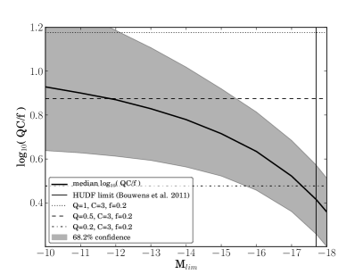
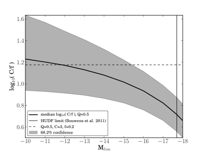
We can make further progress by adopting a prior on . Recent theoretical calculations suggest that is of order 1-6, and we therefore assume a uniform prior within this range. Very little empirical or theoretical information is available on the escape fraction. We formalize the uncertainty on this parameter by assuming a uniform prior in the range (e.g., Fernandez & Shull, 2011). With these priors we derive the joint constraints on and Mlim shown in Figure 11. Figure 11 shows that allowing for a larger range in and increases the available ranges of for the BoRG13 luminosity function. However, even here only for the most extreme combination of and at there seems to be enough radiation available to sustain a fully ionized Universe at . Overall it is clear from Figures 10 and 11 that reionization is far from being completed at by an LBG population following the BoRG13 5 luminosity function. Invoking a luminosity function with a steeper faint-end slope (e.g., the BoRG13 8 luminosity function) changes this picture somewhat. However, still requires radiation from objects down to , as supported by non-detection of gamma-ray burst host galaxies at (Trenti et al., 2012a; Tanvir et al., 2012) and therefore still supports a late reionization, i.e., that reionization completes at .
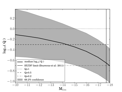
We can compare our inference on with the values inferred from the measured Ly optical depth as inferred from spectroscopic follow-up of Y-band dropouts (e.g., Treu et al., 2013). Naturally this comparison is extremely delicate and needs to rely on a number of assumptions, as the Ly optical depth depends not only on the average fraction of neutral hydrogen in the IGM but also on the details of the Ly emission itself and on the detailed radiative transfer at or in the vicinity of the source (e.g., Dijkstra et al., 2011; Bolton & Haehnelt, 2013). Several authors have suggested that ionized fractions of are needed to explain the observed decline in Ly emission from LBGs between and , if all the optical depth arises from neutral hydrogen in the IGM and if the universe is completely reionized by . Our recent follow-up of a subsample of the BoRG LBGs with MOSFIRE (Treu et al., 2013) indicates that the optical depth increases even more out to , indicating perhaps an even lower fraction of ionized hydrogen, which seems to be in good agreement with the results summarized in Figures 10 and 11. However, given the extreme assumptions, these numbers should be considered lower limits to the cosmic average fraction of neutral hydrogen. In order to gain some insight into we can adopt as our upper limit and infer our exclusion plots in versus Mlim shown in Figure 12.
In summary the inferred luminosity function from the BoRG13 data is not capable of fully ionizing the Universe at redshift as a significant fraction of neutral hydrogen seems to still be present. This is in good agreement with recent results from spectroscopic follow-up campaigns which all seem to suggest that a significant fraction of neutral hydrogen is present at . Hence, the results presented here support a late reionization scheme where the reionization is still ongoing at .
6. Summary and conclusion
The BoRG survey has carried out the largest-area search to date for Y-band dropouts (HST F098M-dropouts). We present new observations from 12 parallel fields not included in our previous studies and additional deeper datasets for two fields. We combine our BoRG sample with a sample of fainter dropouts taken from the literature and use the combined sample of dropouts to carry out a rigorous study of the luminosity function at and its implications for reionization. Our main results can be summarized as follows:
-
1.
We present 9 new Y-band dropouts from the 50 arcmin2 of new data. Furthermore, we re-confirm two dropouts previously presented by Trenti et al. (2011) and Bradley et al. (2012). Combining these 11 dropouts with out previously published LBGs from BoRG gives a sample of 38 bright () redshift 8 LBGs from the BoRG survey.
-
2.
We develop and implement an improved method for estimating the luminosity function parameters for a sample of galaxies. Using a Bayesian framework the posterior distribution of the population based on a binomial distribution is given. Combining the BoRG Y-band dropouts with the faint LBGs from HUDF/ERS presented by Bouwens et al. (2011) and sampling over this posterior distribution enables a robust recovery of the faint-end slope, , the characteristic magnitude of the Schechter function, , the normalizing number density of LBGs, , and the luminosity density, , of the redshift 8 luminosity function.
-
3.
The inferred luminosity function at is described by the parameters:
-
,
-
,
-
,
-
Here is the inferred UV luminosity density integrated down to the HUDF limit M. Our inferred credible intervals include recent estimates of the same parameters.
-
-
4.
We show that for the BoRG13 luminosity function the average fraction of ionized hydrogen is only of the order 10-50% for samples down to the HUDF limit of assuming standard values of the clumping factor and the photon escape fraction. To sustain a fully ionized Universe at redshift 8 with the presented luminosity function it is necessary to account for the radiation of objects as faint as .
-
5.
The inferred ionization fractions suggest a relatively late reionization scenario where a considerable fraction of neutral hydrogen is still present at in good agreement with the results of our recent spectroscopic MOSFIRE campaign (and others from the literature) where we followed up a subsample of the BoRG redshift 8 LBGs presented here.
The inference on the implications of the BoRG13 luminosity function for reionization presented here are still limited by the sizable error bars at redshift 8. To reduce the uncertainties on the inferred quantities bright and faint galaxy samples from e.g., the Frontier Fields and future parallel HST campaigns are crucial.
Appendix A HST-GO Follow-Up of BoRG_1437+5043
The BoRG_1437+5043 field is a special case, and thus its analysis deserves a detailed description. The field was originally identified by Trenti et al. (2012b) as an overdensity of 4 Y-band dropouts detected above the limit and 1 detected above . As explained in that work, overdensitites of high redshift galaxies are expected to occur from theoretical and numerical dark matter modeling. It was thus argued that the overdensity could potentially be a high redshift protocluster. Bradley et al. (2012) subsequently carried out a re-analysis of the field. With improved data reduction and photometry algorithms, 2 out of the 4 initial 5 candidates presented by Trenti et al. (2012b) fell below the formal 5 threshold. The 8 candidate was confirmed.
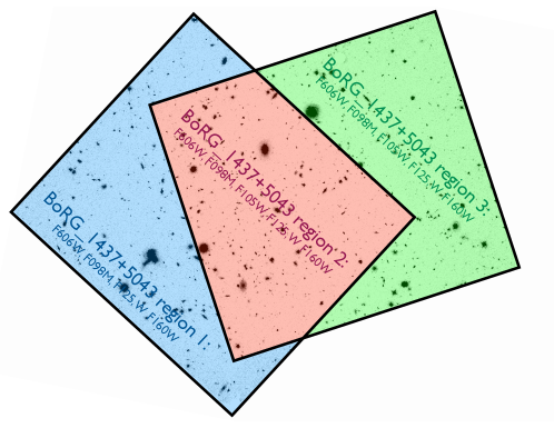
In order to further investigate the nature of the sources in this field, follow-up observations were proposed for and obtained in November 2012 . The main goal of the new HST campaign (GO 12905, PI: Trenti) was to look for fainter members of the overdensity as well as expand the area surveyed by centering the field directly on the overdensity. The GO data was taken in the 4 original photometric bands of the BoRG survey, F606W, F098M, F125W, and F160W, plus F105W in order to sharpen the redshift estimate of the dropout candidates. In Figure 13 we show the combined J-band image of BoRG_1437+5043. The three differently colored regions mark regions with similar depth and band coverage. The filters used in each region are listed. Regions 1 and 2 outline the original area of the BoRG_1437+5043 field analyzed by Trenti et al. (2012b). Regions 2 and 3 show the position of the new data. Hence, region 2 centered on the potential protocluster contains the deepest data.
The new GO observations were reduced and analyzed together with the rest of the BoRG13 data as presented in this paper. Each of the three regions were analyzed independently in order to accommodate the different depth and band coverage. The limiting magnitudes of each of the three regions are listed in Table 1 together with the rest of the BoRG13 fields. Photometry at the location of the five sources identified by Trenti et al. (2012b) is given in Table 5. We note that the two dropouts that were not confirmed in the reanalysis carried out by Bradley et al. (2012) are indeed not high-z candidates according to the deeper data, thus confirming the improvements introduced in the BoRG pipeline.
Postage stamps at the location of the three candidates retained by Bradley et al. (2012) are shown in Figure 14 along with their photometric redshift estimates. As we can see from the photo- estimates, 2 of the 3 candidates are confirmed to be at , even though one of them (T12e) falls just outside of the formal Y-H color selection criterion. T12a is now detected at S/N in the J(H) band and T12e is detected at S/N. They are thus both excellent redshift candidates. The third candidate (T12b) is undetected in the deeper data and thus we conclude it was a spurious noise peak. The beautifully sharp photo- of the initial 8 candidate T12a is a nice validation of the reliability of the high-significance sample where . As we show in the next section the distribution of noise and background is highly non-Gaussian, so it is not surprising that a fraction of sources just above the 5 threshold are spurious. The 2/3 confirmed fraction is consistent with the fiducial contamination fraction of 42% that we adopt in our inference based on numerical simulations.
Albeit, with admittedly small number statistics this follow-up campaign validates our approach of carrying out separately the inference for the more robust 8 detections and comparing the results with those based on the 5 sample for which contamination is expected to be higher. No fainter candidates are detected in the field. These results imply that the field is still likely to be an overdensity of but not as pronounced as previously thought.



| ID | J | Y J | J H | S/N | S/N | S/N | S/N | Sample | ||
| B1437_r2_0637_T12a | 219.21058 | 50.72601 | 25.76 0.07 | 3.19 0.78 | 0.07 0.11 | 1.0 | 20.2 | 16.5 | BoRG13 | |
| BoRG12 | ||||||||||
| 219.2107 | +50.7260 | - | - | 13.0 | 8.0 | BoRG09 | ||||
| B1437_r2_T12b | 219.22405* | 50.72597* | - | - | - | - | - | - | - | BoRG13 |
| BoRG12 | ||||||||||
| 219.2241 | +50.7260 | - | - | 5.1 | 2.6 | BoRG09 | ||||
| B1437_r2_0560_T12c | 219.23092 | 50.72405 | 27.75 0.23 | 0.83 0.47 | 0.06 0.33 | 3.5 | 2.6 | 6.1 | 5.0 | BoRG13 |
| BoRG12 | ||||||||||
| 219.2311 | +50.7241 | - | - | 5.5 | 2.7 | BoRG09 | ||||
| B1437_r2_T12d | 219.22027* | 50.71563* | - | - | - | - | - | - | - | BoRG13 |
| BoRG12 | ||||||||||
| 219.2203 | +50.7156 | - | - | 5.4 | 2.7 | BoRG09 | ||||
| B1437_r2_0070_T12e | 219.22225 | 50.70808 | 26.91 0.14 | 1.53 0.49 | 0.24 | 0.8 | 2.1 | 9.4 | 7.0 | BoRG13 |
| BoRG12 | ||||||||||
| 219.2224 | +50.7081 | - | - | 6.0 | 2.9 | BoRG09 | ||||
| Note. – Columns are the same as in Table 2 except for the last column which shows where the data were taken from. The ‘T12x’ subscript | ||||||||||
| in the IDs refers to the candidate’s designation in Trenti et al. (2012b) Figure 3. *Coordinates taken from Bradley et al. (2012) as objects | ||||||||||
| are not in the BoRG13 SExtractor segmentation maps. | ||||||||||
Appendix B Non-gaussian noise distribution and the importance of multi-band selection
When quoting ‘3’ or ‘5’ detections in dropout surveys, as well as other areas of astrophysics, it may be implicitly assumed that the noise of the science images is Gaussian distributed such that a 3 and 5 detection corresponds to a probability of the detection being real of 99.730020% and 99.999943%. For a million independent apertures, like those in the BoRG survey, this would correspond to 2700 and 0.57 objects, respectively, and thus effectively no contaminants in a 5 sample, even for an area as large as the one surveyed by BoRG.
In practice, however, we do not expect the noise distribution to be Gaussian. Furthermore, we do not expect it to be symmetric. This is in part due to unresolved background objects but also due to the positive nature of defects such as faint cosmic ray hits and hot pixels. Thus, when the data are pushed to the limit as in dropout searches for Lyman break galaxies, the non-Gaussian tails of the noise distributions can result in false positive detections (e.g., Dunlop, 2013) even if they are formally 5 detections.
In this appendix we take advantage of the very large area covered by the BoRG Survey to characterize and demonstrate the non-Gaussianity of the background. We show that the level of contaminants is much higher than for a Gaussian background, and that only through the use of multiple filters for detections and non-detection requirements it can be kept at the relatively manageable level of 42%.
We construct the actual probability distribution function of
background noise by conducting aperture photometry on all possible
apertures of radius from the empty regions in 71 of
the BoRG fields. Empty regions are identified according to the
SExtractor segmentation maps (grown by 5 pixels) produced when
creating our source catalogs as described in Section 3.
We note that the correlated noise introduced by the drizzling of the science images
is automatically accounted for by this approach.
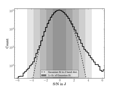
In Figure 15 we show the distribution of S/N values
for all apertures in the J-band (left) and the J-H-band 2D S/N
histogram for objects with S/N (right). The dashed
line in the left panel shows a Gaussian fit to the J-band distribution
of the empty apertures. Is is clear that the one-dimensional
distribution of the noise apertures has broader tails than would be
expected for a Gaussian distribution.
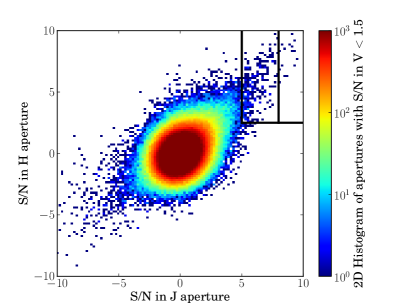
The majority of the potential false positives are rejected by our multi-band requirements: a ‘5’ detection in J as well as a ‘2.5’ detection in the H-band and a non-detection in the V band (S/N). This selection is illustrated by the box in the upper right corner of the right panel in Figure 15. In spite of the three band selection, still 479 empty apertures survive the cuts, i.e. 7 per BoRG field. The 8 requirement on J is more stringent but still leaves 65 apertures, i.e. approximately one per BoRG field.
However, as mentioned in Section 3 a crucial part of the dropout selection is the color cut on . Applying this stringent cut removes all of the noise peaks passing the S/N cuts. This can be understood as the results of two effects in the BoRG data. First, the vast majority of sources in the sky are not as red, and therefore the population with fluxes just below our detection threshold which happens to be upscattered in the sample by noise fluctuations is unlikely to satisfy this requirement. Second, spurious positive signals like hot pixels will be present in all near-infrared bands in undithered data and therefore requiring much fainter flux in Y than J helps eliminate those as well. We note that the BoRG survey by design takes all three near-infrared exposures in the same orbit to maximize the chances that hot pixels and detector persistence create images in both the Y-band (taken first), J-band and H-band image. Hence, such artifacts should not be selected as Y-band dropouts in the BoRG survey.
From this study of the noise distribution we draw the following conclusions. Potential contaminants abound in 5 samples, and multiple band detections are essential to keep them under control. Thus, it is to be expected that repeated observations of the same field will yield different sets of marginal candidates, like in the case of the BoRG_1437+5043 field. Higher significance 8 samples are much more reliable, but still not immune to noise fluctuation. In addition to carrying out and comparing analyses for both and 8 samples it is therefore essential to impose strict color cuts, or impose equivalently tight photo- requirements. This naturally reduces the completeness of the samples, but it is a reasonable price to pay as long as the completeness can be properly accounted for by means of detailed simulations.
Appendix C Bayesian Luminosity Function Inference Framework
In this appendix we outline the Bayesian framework used to infer the parameters of the intrinsic luminosity function in this study. Before describing the posterior distribution used for the MCMC sampling we describe how the individual parameters are related under the assumption of a Schechter luminosity function.
C.1. The Schechter Luminosity Function and its Parameters
The luminosity function of a sample of galaxies represents the density of objects in a given co-moving volume as a function of the luminosity. Hence, it gives information about the population of galaxies at a certain redshift and can be integrated to reveal the total number of galaxies. For luminosity functions at higher redshift this becomes interesting as this gives a direct measure of the reionization power of the galaxies at the given epoch and therefore aid the understanding of which sources reionized the Universe and by how much and when the majority of reionization happened. The Schechter function (Schechter, 1976) is one of the most widely used luminosity function models. The Schechter function is given by
| (C1) |
where is the so-called shape parameter. is the so-called ‘faint-end slope’ of the luminosity function that is analyzed in the present study. is the scale parameter that determines the transition between the power-law behavior of Equation (C1) that dominates at low luminosities and the exponential cut-off at the bright end. is a normalizing co-moving number density of objects. The Schechter function is closely related to the gamma distribution as
| (C2) |
with being the gamma function which is defined as
| (C3) |
Formally the integral of the gamma (Schechter) function diverges for . This problem is circumvented by introducing a minimum luminosity, , instead of integrating from 0. As the concept of galaxies is only valid above a certain luminosity this approximation is physically motivated. For instance a galaxy of makes no physical sense. An often used “definition” of a galaxy is an object with an absolute magnitude which corresponds to a luminosity of erg/s which is roughly times the energy output of the Sun. Limiting the integration of the gamma functions makes it the incomplete gamma function.
The normalizing galaxy density, , is closely related to the total number of galaxies present in the surveyed volume of the Universe following the given luminosity function. As noted above, the luminosity function can be integrated to reveal the total number of galaxies, , within the effective co-moving volume given the number density such that
| (C4) | |||||
which assumes that the luminosity function does not evolve over the considered redshift interval. The effective co-moving volume can be determined as
| (C5) |
where is the cosmological volume element and p(z) is the probability of selecting the objects for a given redshift in the surveyed redshift range; essentially a selection function. For an evolving luminosity function the integral in Equation (C4) is done over separately.
In a similar manner it is possible to obtain the luminosity density, , i.e., the available radiation per volume, radiated by the galaxy sample, by integrating the product of the luminosity function and the luminosity such that
| (C6) |
Hence, the three key parameters to determine when characterizing the luminosity function of a sample of galaxies are , and (or similarly , and ). In the following we will described the marginal posterior distribution we used to obtain these parameters.
C.2. The Marginal Posterior Distribution
From Bayesian statistics it is known that the posterior probability distribution is proportional to the product of the prior distribution and the likelihood. When determining the luminosity function of samples of high redshift objects, what is usually done is essentially to assume that everything is detected above a certain luminosity threshold, which in the case of the objects we deal with here, is the detection threshold in the J-band, under the assumption that each object is not detected in V. Thus the relationship between the posterior and prior probability distribution for the high-redshift galaxy candidates can be expressed as
| (C7) |
where the last term is the likelihood. contains the parameters describing the luminosity function , is the observed luminosity in the J-band with being the true luminosity, and indicates whether the observed luminosity in the V-band represents a formal detection () or not (). For an object to be included in the sample it cannot be detected in the V-band so is always the case. contains any prior information on the luminosity function parameters that might be available. In the present study we assume uniform priors on , and .
Expanding the expression for the posterior in Equation (C7) marginalizing over the nuisance parameter (the true luminosity of the object in the J-band) leads to a marginal posterior probability distribution for a sample of galaxies which is given by (see Section 3.1 and Appendix B of Kelly et al., 2008):
| (C8) | |||||
where is the number of high- sources in the Universe given the intrinsic luminosity function and is the number of objects which would potentially contaminate the luminosity function. The corresponding values for the observed sample are and where the total number of objects in the galaxy sample is given by . If individual fields are included in the sample this is accounted for by taking the product over the fields where corresponds to the number of objects in the ’th field such that . The ratio gives the fractional area the ’th field covers on the sky. The terms are binomial coefficients which can be expressed in terms of the logarithm of the gamma function as
| (C9) |
The number of contaminants is determined by the contamination fraction . By approximating the number of contaminants by its expectation value such that
Equation (C8) becomes
| (C10) |
Here the contamination varies between each field contributing to the final sample as indicated by the subscript . The term on the right-hand-side represents the probability distribution of an object making it into the sample but is independent on the individual observations. However, it differs between the different observed fields (or surveys) in the sample as exposure times and hence depths differ from field to field. Expanding the detection probability for the considered sample we have that
| (C11) |
Here is the selection function for the ’th field accounted for completeness.
The last term on the right-hand-side in Equation (C10) also appearing in Equation (C11) represents the likelihood of the ’th object in the sample which can be expressed as
Where we use (see Equation (1) of Kelly et al., 2008) and that gamma is related to the Schechter luminosity function as shown in Equation (C2).
| (C13) |
represents the true luminosity inferred from the observations assuming a Gaussian measurement error with being the median photometric error in the J-band in the given field.
By denoting the selection function with and defining
| (C14) |
we can express Equation (C10) as
| (C15) | |||||
This is the posterior probability distribution for a sample of objects assumed to be binomially distributed and to have an intrinsic Schechter luminosity function on the form shown in Equation (C1), where each observed luminosity is related to the true luminosity through an assumed Gaussian error distribution and where the prior on is uniform.
Estimating for a certain corresponds to estimating the probability that the luminosity function with the parameters is the intrinsic luminosity function of the analyzed galaxy sample. The intrinsic luminosity function can for instance be obtained from this expression by sampling via a Markov Chain Monte Carlo approach. As described in Section 4 we used such an approach to infer the intrinsic luminosity function at redshift 8 for the BoRG13 sample.
Having obtained the three-dimensional posterior distribution for the number density of high redshift galaxies, , and the luminosity density, , can be determined using Equations (C4) and (C6). The current framework assumes that the fraction of contaminants is independent of luminosity for the BoRG sample.
Above we have partially followed Kelly et al. (2008) and refer to this work for further details.
References
- Baker & Menzel (1938) Baker, J. G., & Menzel, D. H. 1938, Astrophysical Journal, 88, 52
- Benítez et al. (2004) Benítez, N., Ford, H., Bouwens, R., et al. 2004, The Astrophysical Journal Supplement Series, 150, 1
- Bertin & Arnouts (1996) Bertin, E., & Arnouts, S. 1996, Astronomy and Astrophysics Supplement, 117, 393
- Bolton & Haehnelt (2013) Bolton, J. S., & Haehnelt, M. G. 2013, Monthly Notices of the Royal Astronomical Society, 429, 1695
- Bouwens et al. (2004) Bouwens, R. J., Illingworth, G. D., Blakeslee, J. P., Broadhurst, T. J., & Franx, M. 2004, The Astrophysical Journal, 611, L1
- Bouwens et al. (2006) Bouwens, R. J., Illingworth, G. D., Blakeslee, J. P., & Franx, M. 2006, The Astrophysical Journal, 653, 53
- Bouwens et al. (2007) Bouwens, R. J., Illingworth, G. D., Franx, M., & Ford, H. 2007, The Astrophysical Journal, 670, 928
- Bouwens et al. (2010) Bouwens, R. J., Illingworth, G. D., Oesch, P. A., et al. 2010, The Astrophysical Journal Letters, 709, L133
- Bouwens et al. (2011) —. 2011, The Astrophysical Journal, 737, 90
- Bouwens et al. (2012) —. 2012, The Astrophysical Journal Letters, 752, L5
- Bradley et al. (2012) Bradley, L. D., Trenti, M., Oesch, P. A., et al. 2012, The Astrophysical Journal, 760, 108
- Bradley et al. (2013) Bradley, L. D., Zitrin, A., Coe, D., et al. 2013, eprint arXiv, 1308, 1692
- Cai et al. (2014) Cai, Z.-Y., Lapi, A., Bressan, A., et al. 2014, eprint arXiv, 1403, 55
- Capak et al. (2013) Capak, P., Faisst, A., Vieira, J. D., et al. 2013, The Astrophysical Journal Letters, 773, L14, accepted to ApJL, 5 Pages, 4 Figures, 1 Table
- Cara & Lister (2008) Cara, M., & Lister, M. L. 2008, The Astrophysical Journal, 686, 148
- Cardelli et al. (1989) Cardelli, J. A., Clayton, G. C., & Mathis, J. S. 1989, Astrophysical Journal, 345, 245
- Caruana et al. (2012) Caruana, J., Bunker, A. J., Wilkins, S. M., et al. 2012, Monthly Notices RAS, 427, 3055
- Caruana et al. (2013) —. 2013, eprint arXiv, 1311, 57, submitted to MNRAS
- Casertano et al. (2000) Casertano, S., de Mello, D., Dickinson, M., et al. 2000, The Astronomical Journal, 120, 2747
- Coe et al. (2006) Coe, D., Benítez, N., Sánchez, S. F., et al. 2006, The Astronomical Journal, 132, 926
- Dijkstra et al. (2011) Dijkstra, M., Mesinger, A., & Wyithe, J. S. B. 2011, Monthly Notices of the Royal Astronomical Society, 414, 2139
- Dunlop (2013) Dunlop, J. S. 2013, The First Galaxies, 396, 223
- Dunlop et al. (2012a) Dunlop, J. S., McLure, R. J., Robertson, B. E., et al. 2012a, Monthly Notices RAS, 420, 901
- Dunlop et al. (2012b) Dunlop, J. S., Rogers, A. B., McLure, R. J., et al. 2012b, eprint arXiv, 1212, 860, 13 pages, 7 figures, submitted to MNRAS
- Ellis et al. (2012) Ellis, R. S., McLure, R. J., Dunlop, J. S., et al. 2012, eprint arXiv, 1211, 6804
- Faisst et al. (2014) Faisst, A. L., Capak, P., Carollo, C. M., Scarlata, C., & Scoville, N. 2014, eprint arXiv, 1402, 3604, 11 pages, 6 figures, 2 tables, submitted to ApJ
- Ferguson et al. (2004) Ferguson, H. C., Dickinson, M., Giavalisco, M., et al. 2004, The Astrophysical Journal, 600, L107
- Fernandez & Shull (2011) Fernandez, E. R., & Shull, J. M. 2011, The Astrophysical Journal, 731, 20
- Finkelstein et al. (2010) Finkelstein, S. L., Papovich, C., Giavalisco, M., et al. 2010, The Astrophysical Journal, 719, 1250
- Finkelstein et al. (2012) Finkelstein, S. L., Papovich, C., Salmon, B., et al. 2012, The Astrophysical Journal, 756, 164
- Finkelstein et al. (2013) Finkelstein, S. L., Papovich, C., Dickinson, M., et al. 2013, eprint arXiv, 1310, 6031
- Finlator et al. (2012) Finlator, K., Oh, S. P., Özel, F., & Davé, R. 2012, Monthly Notices of the Royal Astronomical Society, 427, 2464
- Fontana et al. (2010) Fontana, A., Vanzella, E., Pentericci, L., et al. 2010, The Astrophysical Journal Letters, 725, L205
- Grogin et al. (2011) Grogin, N. A., Kocevski, D. D., Faber, S. M., et al. 2011, The Astrophysical Journal Supplement, 197, 35
- Illingworth et al. (2013) Illingworth, G. D., Magee, D., Oesch, P. A., et al. 2013, eprint arXiv, 1305, 1931
- Jaacks et al. (2013) Jaacks, J., Thompson, R., & Nagamine, K. 2013, eprint arXiv, 1301, 5270, 6 pages, 4 figures, submitted
- Kaurov & Gnedin (2013) Kaurov, A. A., & Gnedin, N. Y. 2013, eprint arXiv, 1311, 2594, 6 pages, 5 figures, submitted to ApJ
- Kelly et al. (2008) Kelly, B. C., Fan, X., & Vestergaard, M. 2008, The Astrophysical Journal, 682, 874
- Koekemoer et al. (2003) Koekemoer, A. M., Fruchter, A. S., Hook, R. N., & Hack, W. 2003, The 2002 HST Calibration Workshop : Hubble after the Installation of the ACS and the NICMOS Cooling System, 337
- Koekemoer et al. (2011) Koekemoer, A. M., Faber, S. M., Ferguson, H. C., et al. 2011, The Astrophysical Journal Supplement, 197, 36
- Koekemoer et al. (2012) Koekemoer, A. M., Ellis, R. S., McLure, R. J., et al. 2012, eprint arXiv, 1212, 1448, 16 pages, 9 figures, submitted to ApJS
- Lorenzoni et al. (2011) Lorenzoni, S., Bunker, A. J., Wilkins, S. M., et al. 2011, Monthly Notices RAS, 414, 1455
- Madau et al. (1996) Madau, P., Ferguson, H. C., Dickinson, M. E., et al. 1996, Monthly Notices RAS, 283, 1388
- McLure et al. (2010) McLure, R. J., Dunlop, J. S., Cirasuolo, M., et al. 2010, Monthly Notices of the Royal Astronomical Society, 403, 960
- McLure et al. (2013) McLure, R. J., Dunlop, J. S., Bowler, R. A. A., et al. 2013, Monthly Notices of the Royal Astronomical Society, 432, 2696, 19 pages, 7 figures, submitted to MNRAS
- McQuinn et al. (2011) McQuinn, M., Oh, S. P., & Faucher-Giguère, C.-A. 2011, The Astrophysical Journal, 743, 82
- Oesch et al. (2007) Oesch, P. A., Stiavelli, M., Carollo, C. M., et al. 2007, The Astrophysical Journal, 671, 1212
- Oesch et al. (2009) Oesch, P. A., Carollo, C. M., Stiavelli, M., et al. 2009, The Astrophysical Journal, 690, 1350
- Oesch et al. (2010a) Oesch, P. A., Bouwens, R. J., Carollo, C. M., et al. 2010a, The Astrophysical Journal Letters, 725, L150
- Oesch et al. (2010b) —. 2010b, The Astrophysical Journal Letters, 709, L21
- Oesch et al. (2010c) Oesch, P. A., Bouwens, R. J., Illingworth, G. D., et al. 2010c, The Astrophysical Journal Letters, 709, L16
- Oesch et al. (2012) —. 2012, The Astrophysical Journal, 759, 135
- Oesch et al. (2013) —. 2013, The Astrophysical Journal, 773, 75, 21 pages, 13 figures, 6 tables; submitted to ApJ
- Ono et al. (2012a) Ono, Y., Ouchi, M., Curtis-Lake, E., et al. 2012a, eprint arXiv, 1212, 3869, 15 pages, 13 figures, submitted to ApJ
- Ono et al. (2012b) Ono, Y., Ouchi, M., Mobasher, B., et al. 2012b, The Astrophysical Journal, 744, 83
- Ouchi et al. (2009) Ouchi, M., Mobasher, B., Shimasaku, K., et al. 2009, The Astrophysical Journal, 706, 1136
- Ouchi et al. (2010) Ouchi, M., Shimasaku, K., Furusawa, H., et al. 2010, The Astrophysical Journal, 723, 869
- Reddy & Steidel (2009) Reddy, N. A., & Steidel, C. C. 2009, The Astrophysical Journal, 692, 778
- Robertson et al. (2013) Robertson, B. E., Furlanetto, S. R., Schneider, E., et al. 2013, The Astrophysical Journal, 768, 71
- Schechter (1976) Schechter, P. 1976, Astrophysical Journal, 203, 297, a&AA ID. AAA017.158.009
- Schenker et al. (2013) Schenker, M. A., Robertson, B. E., Ellis, R. S., et al. 2013, The Astrophysical Journal, 768, 196, 15 pages, 5 figures, To be submitted to ApJ
- Shull et al. (2012) Shull, J. M., Harness, A., Trenti, M., & Smith, B. D. 2012, The Astrophysical Journal, 747, 100
- Stark et al. (2010) Stark, D. P., Ellis, R. S., Chiu, K., Ouchi, M., & Bunker, A. 2010, Monthly Notices RAS, 408, 1628
- Stark et al. (2013) Stark, D. P., Schenker, M. A., Ellis, R., et al. 2013, The Astrophysical Journal, 763, 129
- Steidel et al. (2000) Steidel, C. C., Adelberger, K. L., Shapley, A. E., et al. 2000, The Astrophysical Journal, 532, 170
- Steidel et al. (1996) Steidel, C. C., Giavalisco, M., Pettini, M., Dickinson, M., & Adelberger, K. L. 1996, Astrophysical Journal Letters v.462, 462, L17
- Tacchella et al. (2013) Tacchella, S., Trenti, M., & Carollo, C. M. 2013, The Astrophysical Journal Letters, 768, L37
- Tanvir et al. (2012) Tanvir, N. R., Levan, A. J., Fruchter, A. S., et al. 2012, The Astrophysical Journal, 754, 46
- Trenti et al. (2012a) Trenti, M., Perna, R., Levesque, E. M., Shull, J. M., & Stocke, J. T. 2012a, The Astrophysical Journal Letters, 749, L38
- Trenti & Stiavelli (2008) Trenti, M., & Stiavelli, M. 2008, The Astrophysical Journal, 676, 767
- Trenti et al. (2010) Trenti, M., Stiavelli, M., Bouwens, R. J., et al. 2010, The Astrophysical Journal Letters, 714, L202
- Trenti et al. (2011) Trenti, M., Bradley, L. D., Stiavelli, M., et al. 2011, The Astrophysical Journal Letters, 727, L39
- Trenti et al. (2012b) —. 2012b, The Astrophysical Journal, 746, 55
- Treu et al. (2013) Treu, T., Schmidt, K. B., Trenti, M., Bradley, L. D., & Stiavelli, M. 2013, The Astrophysical Journal Letters, 775, L29
- Treu et al. (2012) Treu, T., Trenti, M., Stiavelli, M., Auger, M. W., & Bradley, L. D. 2012, The Astrophysical Journal, 747, 27
- van Dokkum (2001) van Dokkum, P. G. 2001, The Publications of the Astronomical Society of the Pacific, 113, 1420
- Vanzella et al. (2009) Vanzella, E., Giavalisco, M., Dickinson, M., et al. 2009, The Astrophysical Journal, 695, 1163
- Vihola (2012) Vihola, M. 2012, Statistics and Computing
- Yan et al. (2011) Yan, H., Yan, L., Zamojski, M. A., et al. 2011, The Astrophysical Journal Letters, 728, L22
- Yuan & Wang (2013) Yuan, Z., & Wang, J. 2013, eprint arXiv, 1302, 5887
- Zaroubi (2013) Zaroubi, S. 2013, The First Galaxies, 396, 45