Bayesian Inference for NMR Spectroscopy with Applications to Chemical Quantification

Abstract

Nuclear magnetic resonance (NMR) spectroscopy exploits the magnetic properties of atomic nuclei to discover the structure, reaction state and chemical environment of molecules. We propose a probabilistic generative model and inference procedures for NMR spectroscopy. Specifically, we use a weighted sum of trigonometric functions undergoing exponential decay to model free induction decay (FID) signals. We discuss the challenges in estimating the components of this general model – amplitudes, phase shifts, frequencies, decay rates, and noise variances – and offer practical solutions. We compare with conventional Fourier transform spectroscopy for estimating the relative concentrations of chemicals in a mixture, using synthetic and experimentally acquired FID signals. We find the proposed model is particularly robust to low signal to noise ratios (SNR), and overlapping peaks in the Fourier transform of the FID, enabling accurate predictions (e.g., $1$% sensitivity at low SNR) which are not possible with conventional spectroscopy ($5$% sensitivity).

1402.3580

, , ,
, , ,

1 Introduction

Nuclear magnetic resonance (NMR) spectroscopy has greatly advanced our understanding of molecular properties, and is now widespread in analytical chemistry. The theory of nuclear magnetic resonance postulates that protons and neutrons behave like gyroscopes that spin about their axes, generating their own small magnetic fields. These concepts were first described by Rabi et al. (1939), for which Isidor Rabi was awarded the 1944 Nobel prize in physics. Later, Bloch, Hanson and Packard (1946) and Purcell, Torrey and Pound (1946) showed how NMR could be used to understand the structure of molecules in liquids and solids, for which they shared the Nobel prize in physics in 1952. Richard Ernst then won the 1991 Nobel prize in chemistry for developing Fourier transform NMR spectroscopy, which led to the prevalence of NMR as an analytic technique. NMR spectroscopy is well suited to studying both organic and inorganic molecules, including proteins, and other biochemical species (Barrett et al., 2013), and is routinely used to identify the structure of unknown chemical species or the composition of mixtures.

NMR spectroscopy is quantitative, chemically specific and non-invasive and therefore can be used to study molecules in situ (Gladden, 1994). A major limitation of conventional NMR spectroscopy is its low senstivity, which has led researchers to develop ever more powerful magnets to amplify the signal (Barrett et al., 2013). However, stronger magnetic fields have limited returns: they are costly and also impractical in many applications, e.g., plant measurements in the chemical industry (Dalitz et al., 2012). There are therefore strong drivers to develop alternative techniques that can provide chemical information from relatively poor quality data.

In this paper, we propose an alternate approach to NMR spectroscopy. In our approach, we model the free induction decay (FID) signal as a realisation from a probabilistic generative model, and we use Bayesian inference and likelihood principles to infer latent variables in this model. This model allows us to leverage additional information in the FID over conventional Fourier transform spectroscopy, with explicit models of signal decay, phase shifts, frequencies, and noise, and prior information, e.g.  about resonant frequencies.

In a body of pioneering work (Bretthorst, 1990; Evilia, Effiong and Whittenburg, 1993; Dou and Hodgson, 1995; Andrec and Prestegard, 1998; Rubtsov and Griffin, 2007; Hutton et al., 2009; Aboutanios, Kopsinis and Rubtsov, 2012), discussed further in section 6, various statistical models have been proposed to model the FID directly. These models, while promising, have not yet been widely adopted, with practicioners typically preferring conventional Fourier transform spectroscopy. We further pursue the line of research instigated by Bretthorst (1990), to develop a statistical model of the FID which we show can be used as a highly practical tool. In particular, we introduce new modelling parameters (such as time delays), new estimation procedures, detailed stress tests, detailed comparisons with conventional methods, implementational details necessary for good performance, and the application to chemical quantification. In general, our approach is robust to noise, and allows one to study systems in which there is significant overlap between peaks in the Fourier transform of the FID signal, and a large number of resonant frequencies. While most approaches to NMR spectroscopy are applied in the high resolution ${}^{1}\text{H}$ spectrum, we focus on examples in the ${}^{13}\text{C}$ spectrum, which is $10^{4}$ times less sensitive.

We begin with a brief introduction to conventional Fourier transform spectroscopy in section 2. We then introduce our alternative model for free induction decay in section 3, and discuss inference and parameter estimation in this model in sections 4 and 5. We resolve general practical difficulties with parameter estimation in statistical models of free induction decay – difficulties which have not been discussed at length in prior work. In particular, estimating a large number of resonant frequencies, jointly with phase parameters and other variables, requires careful navigation of a highly multimodal likelihood surface.

In our experiments of sections 7 and 8, we compare conventional Fourier transform spectroscopy with the proposed method for predicting the relative concentrations of chemicals in a mixture, using both synthetic and experimentally acquired FID signals. We show that the proposed model enables accurate predictions which are not possible with conventional Fourier transform spectroscopy.

2 Conventional Spectroscopy

In this section we outline a conventional Fourier transform spectroscopy approach (Keeler, 2011; Malz and Jancke, 2005). Then, in the following sections, we will propose an alternative method for NMR spectroscopy, and compare both the conventional and proposed approach for quantifying relative chemical concentrations in a mixture.

To understand how NMR spectroscopy works at a high level, imagine a chemical mixture is placed in a strong magnetic field. Nuclei within this mixture that have non-zero spin will interact with the magnetic field to produce “magnetic moments”. We can imagine these magnetic moments as small bar magnets. Radio frequency (rf) pulses are then directed at the mixture, exerting a torque on these “bar magnets”, causing them to precess perpendicular to the strong magnetic field. The rotating magnets create a magnetic flux through a coil in the NMR machine, which induces a current with periodic components at the resonant frequencies of the chemical mixture. The voltage associated with this current is what is measured in an NMR experiment and is called the free induction decay (FID). The resonant frequencies are sensitive to the local molecular structure, which is what permits NMR to be used as a spectroscopic technique.

In conventional Fourier transform spectroscopy, the FID signal is assumed to be generated by two channels, exactly $\pi/2$ out of phase, with each channel perfectly modelled as a noise free sum of cosines at different frequencies $\omega_{i}^{(j)}$ weighted by intensities $B^{(j)}_{i}$. Thus taking the Fourier transform of the FID, in principle, would result in a series of spikes (delta functions) at the resonant frequencies, and the relative magnitudes of these spikes (after adjusting for the intensities $B^{(j)}_{i}$) would be the relative concentrations of chemicals in a mixture. However, in actuality, there is decay in the signal due to, e.g., variations in the magnetic field (Keeler, 2011) (see also section 3 for more detail). Moreover, the trigonometric terms are not in phase, and there is noise in the signal. In section 3, we explicitly model these properties of the FID.

Throughout our experiments we will consider mixtures of cyclohexane and butanone, so we will exemplify the variant of conventional Fourier transform spectroscopy we use in this context; for reference, we follow the general conventional procedure outlined in Keeler (2011) and Malz and Jancke (2005). Table 1 gives the theoretical intensities $B^{(j)}_{i}$ and frequencies $\omega_{i}^{(j)}$ for cyclohexane and butanone. Because the NMR spectrometer can only excite spins within a certain resonance frequency range, the extent to which each chemical group is excited differs from each other slightly, and this discrepancy is described by what is known as an excitation profile. This phenomenon alters the known intensities $B^{(j)}_{i}$. We therefore run a calibration experiment to measure the excitation profile, analogous to slice excitation measurements in magnetic resonance imaging (Haacke et al., 1999). We then adjust the theoretical intensity values accordingly. The calibrated $B^{(j)}_{i}$ are listed in Table 1. In a given experiment, the resonant frequencies will somewhat differ from those given in Table 1, depending on, for example, the composition of the mixture in question. In a conventional procedure, one must look for peaks near tabulated reference frequencies, and choose which chemical they are associated with. By contrast, the proposed method in the next sections automatically estimates the resonant frequencies for a given chemical mixture.

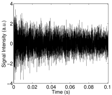
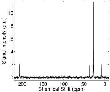
Let $y(t)$ be a given FID signal, as shown in Figure 1. We Fourier transform $y(t)$ using the Discrete Fourier Transform (DFT) to obtain $\tilde{y}(\omega)$, as in Figure 1. The conventional procedure is then to search for each peak near an expected resonant frequency. Since the FID undergoes decay, is noisy, etc., and thus does not perfectly conform to the assumptions of a DFT, there will be width about each peak (e.g., the peaks are not delta function spikes, but look more like Gaussian or Cauchy densities), noise, and overlapping peaks which can be hard to differentiate in practice, particularly given that resonant frequencies will shift in a mixture, as seen in Figure 1.

Figure 1: Conventional Fourier Transform Spectroscopy for a 50-50 mixture of 2-butanone and cyclohexane. a) Free Induction Decay (FID) Signal. b) Discrete Fourier Transform of FID.

Following standard procedure, we identify a peak window for each resonant frequency and sum together the intensity of $\tilde{y}(\omega)$ within this peak window. The summed intensity is then assigned as the total intensity for this peak window. Chemical quantification predictions are sensitive to the peak window, which is chosen heuristically (Malz and Jancke, 2005). Thereafter we are left with $K$ peaks, belonging to chemical $j$, indexed as $S_{k}^{(j)}$. We then calculate

$$I_{j}=\sum_{k}\frac{S_{k}^{(j)}/B_{k}^{(j)}}{K}\,,$$ (2.1)

where $B_{k}^{(j)}$ is the adjusted intensity in Table 1. Using this conventional approach, the concentration of the $j^{\text{th}}$ chemical in the mixture is then calculated as

$$C_{j}=I_{j}/\sum_{j}I_{j}\,.$$ (2.2)

We estimate an error $E_{j}$ on this estimate $C_{j}$ using

$$E_{j}=C_{j}\sqrt{(\frac{E_{I_{j}}}{I_{j}})^{2}+\frac{\sum_{j}E_{I_{j}}^{2}}{(\sum_{j}I_{j})^{2}}}\,,$$ (2.3)

where

$$E_{I_{j}}=\sqrt{\sum_{k}\frac{n_{k}^{(j)}\sigma_{S}^{2}}{(KB_{k}^{(j)})^{2}}}\,.$$ (2.4)

$n_{k}^{(j)}$ is the number of samples along the frequency axis used to defined a peak window for the $k^{\text{th}}$ peak of the $j^{\text{th}}$ chemical (e.g., the number of samples used to calculate $S_{k}^{(j)}$), and $\sigma_{S}$ is the standard deviation of the noise in the spectral domain $\tilde{y}(s)$.

In short, using a conventional Fourier transform spectroscopy method we calculate the relative concentration of chemical $j$ as $C_{j}$ in Eq. (2.2), and the uncertainty about this estimate as $2E_{j}$ in Eq. (2.4) to approximate a 95% credible interval.

Finally, the signal to noise ratio (SNR) of the FID, which we will refer to in the experiments of sections 7 and 8, is given as

$$\text{SNR}=\frac{S_{k}^{(j)}}{B_{k}^{(j)}\sigma_{S}}\,.$$ (2.5)

Using the definition of Eq. (2.5), the SNR will be different for each peak $S_{k}^{(j)}$. When we quote the SNR, we always state the value for the lowest intensity peak.

In both simulations and real experiments, we consider the FID sampled at $4029$ points at $25\mu s$ intervals. For conventional Fourier transform spectroscopy, the time domain data were first apodised with an exponential function and zerofilled to 16384 points to allow a sufficient spectral resolution. Then, a Fourier transform was applied to the FID. A standard baseline correction was then performed on the spectrometer: we fit a polynomial to the Fourier transform of the FID (the spectrum), and subtract the polynomial fit from the spectrum to product a flat baseline. All such conventional processing was performed in TopSpin (Bruker).

Table 1: Resonant frequencies and known intensities for each chemical group in the mixture. The frequencies and theoretical $B^{(j)}_{i}$ are tabulated from the National Institute of Advanced Industrial Science and Technology Database: http://sdbs.riodb.aist.go.jp.

Chemical	Frequencies (ppm)	Excitation profile weighting	Theoretical $B^{(j)}_{i}$	Calibrated $B^{(j)}_{i}$
2-Butanone	$209.29$	$90.79\%$	$1$	$0.908$
	$36.87$	$96.71\%$	$1$	$0.967$
	$29.43$	$95.72\%$	$1$	$0.957$
	$7.87$	$93.03\%$	$1$	$0.93$
Cyclohexane	$27.1$	$95.59\%$	$6$	$5.735$

3 Proposed Model Specification

We now propose an alternative to conventional Fourier transform methods for NMR spectroscopy.

Ultimately, we wish to predict the relative concentrations of chemicals in a mixture, from a time-varying free induction decay (FID) signal. Typically the FID is recorded in two channels, $y_{1}(t)$ and $y_{2}(t)$, assumed $\pi/2$ out of phase (e.g., real and imaginary parts of a complex signal), and independently corrupted with i.i.d. Gaussian white noise.

Assuming $r$ chemical species in a mixture, we model $y_{1}(t)$ as

$$y_{1}(t) =A_{1}\sum_{i=1}^{m_{1}}B_{i}^{(1)}\cos((\omega_{i}^{(1)}-\omega_{0})(t+\tau)+\theta)e^{-\alpha t}+\dots$$

$$+A_{r}\sum_{i=1}^{m_{r}}B_{i}^{(r)}\cos((\omega_{i}^{(r)}-\omega_{0})(t+\tau)+\theta)e^{-\alpha t}$$

$$+\epsilon_{1}(t)\,,$$ (3.1)

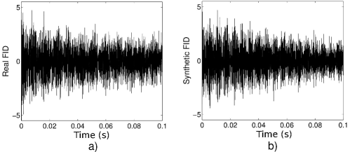
with amplitudes $A_{1},\dots,A_{r}$, frequencies $\{\omega\}_{i}^{(j)}$ and reference frequency $\omega_{0}$ in rad/s (chemical species $j$ has $m_{j}$ resonant frequencies), intensities $\{B\}_{i}^{(j)}$, decay constant $\alpha$ in 1/s, global phase shift $\theta$ in rad, time delay $\tau$ in s, and noise $\epsilon_{1}(t)\sim\mathcal{N}(0,v)$. We will always assume that the intensities $\{B\}_{i}^{(j)}$ and reference frequency $\omega_{0}$ are known and fixed, and we will estimate all other parameters in a procedure outlined in sections 4 and 5. In Figure 2 we show a draw from this generative model, compared with a real FID signal, for a 30% cyclohexane 70% 2-butanone mixture. The real and synthetic FID signals are qualitatively similar – similar resonant frequencies, similar decay rates, etc.

The parameters in the generative model of Eq. (3.1) have clear physical interpretations. The excitation of a sample, e.g. a chemical mixture, in NMR is provided by a radiofrequency (rf) coil which resonates at the frequency of the nucleus of interest, e.g. ¹³C. The time delay $\tau$ in our model arises from the ‘ringdown’ time of this rf coil. The ringdown time is the time taken for the current in the coil to cease. In NMR, rf coils are designed for maximum sensitivity and therefore resonate for a prolonged period after the current supplied to the coil is stopped. The signal from the sample cannot be detected until this ringdown period has finished. In a typical coil this time will be on the order of a few microseconds. In conventional Fourier transform spectroscopy, this delay between excitation and starting the signal detection leads to a linear change in the phase of the signal with frequency variation, which is corrected after Fourier transformation of the raw signal. In our system, we include the time delay in the model directly.

The signal lifetime in NMR is limited by both the relaxation and homogeneity of the magnetic field in which the sample is placed. Both of these effects lead to the decay $\alpha$ of the signal amplitude over time. In an ideal system, the signal will decay through an exponential process (Keeler, 2011). Perhaps surprisingly, this model is also appropriate to a range of non-ideal systems including, e.g., the signal from liquids in rocks (Chen et al., 2005). Here we study pure liquids and so the exponential decay model is most appropriate, though we note that our methodology could easily be adapted for a variety of other models describing the signal decay.

Figure 2: a) Real (experimental) and b) Synthetic free induction decay signals for a 30% cyclohexane 70% 2-butanone mixture, sampled at 25$\mu s$ intervals, from a single channel.

We can rewrite Eq. (3.1) as an inner product of amplitude coefficients $\bm{a}=(A_{1},\dots,A_{r})^{\top}$ with cosine basis functions $\bm{\phi}=(\phi_{1},\dots,\phi_{r})$ parametrized by $\psi=\{\{\omega\}_{i}^{j},\theta,\tau,\alpha\}$:

$$y_{1}(t) =\bm{a}^{\top}\bm{\phi}(t,\psi)+\epsilon_{1}(t)\,,$$ (3.2)

$$\epsilon_{1}(t) \sim\mathcal{N}(0,v)\,.$$ (3.3)

The model for $y_{2}(t)$ is the same,

$$y_{2}(t) =\bm{a}^{\top}\bm{\varphi}(t,\psi)+\epsilon_{2}(t)\,,$$ (3.4)

$$\epsilon_{2}(t) \sim\mathcal{N}(0,v)\,,$$ (3.5)

except we use sine instead of cosine basis functions in $\bm{\varphi}$ to account for the $\pi/2$ phase difference between the two channels.

In section 4 we infer $p(\bm{a}|\mathcal{D},\{t_{n}\}_{n=1}^{N},\psi,v)$, a posterior distribution over the amplitude variables given an observed FID signal $\mathcal{D}$ at times $\{t_{n}\}_{n=1}^{N}$, and nuisance variables $\psi$ and $v$. Since the relative concentrations of chemicals $i$ and $j$ is given by $|A_{i}/A_{j}|$, this posterior distribution can be used to estimate, with uncertainty intervals, the relative concentrations of chemicals in a mixture.

In section 5 we discuss estimation of frequency variables $\{\omega\}_{i}^{(j)}$, other nuisance variables in $\psi$, and the noise variance $v$. Performance in estimating chemical concentrations is especially sensitive to frequency estimates. Moreover, accurately estimating frequency parameters is difficult because the likelihood of the data is highly multimodal as a function of these frequency variables.

Incidentally, it may be a slight misnomer to refer to $\psi,v$ as nuisance variables. Although we are primarily interested in estimating the relative concentrations of chemicals in a mixture – and thus, the $\bm{a}$ variable – the learned frequencies, decay rates, phase shifts, and noise variance are all still enlightening. For instance, the learned frequencies could be used, in principle, to better understand how resonant frequencies shift for particular chemicals when immersed in a mixture.

4 Inference over Amplitudes

We wish to infer $p(\bm{a}|\bm{y}_{1},\bm{y}_{2},\psi,v)$, where $\bm{y}_{1}$ and $\bm{y}_{2}$ are the “real” and “imaginary” channels respectively observed at times $\{t_{1n}\}_{n=1}^{N}$ and $\{t_{2m}\}_{m=1}^{M}$. To reflect our prior uncertainty over the amplitudes, we specify a prior $p(\bm{a})=\mathcal{N}(\mu_{0},S_{0})$, and find

$$p(\bm{a}|\bm{y}_{1},\bm{y}_{2},\psi,v)=\mathcal{N}(\mu,S)\,,$$ (4.1)

$$S=(S_{0}^{-1}+\frac{1}{v}\Phi^{\top}\Phi+\frac{1}{v}\Psi^{\top}\Psi)^{-1}\,,$$ (4.2)

$$\mu=S(S_{0}^{-1}\mu_{0}+\frac{1}{v}\Phi^{\top}\bm{y}_{1}+\frac{1}{v}\Psi^{\top}\bm{y}_{2})\,,$$ (4.3)

where $\Phi$ and $\Psi$ are respectively $N\times r$ and $M\times r$ matrices with entries

$$\Phi_{i,j}(\psi,t_{i})=\bm{\phi}_{j}(\psi,t_{1i})\,,$$ (4.4)

$$\Psi_{i,j}(\psi,t_{i})=\bm{\varphi}_{j}(\psi,t_{2i})\,.$$ (4.5)

We may not know anything about the relative concentrations of the chemicals a priori, in which case we wish to have a vague uninformative prior over the amplitudes. For example, one can use an improper uniform prior on the amplitudes by taking $S_{0}=\lim_{\gamma\to\infty}\gamma I$, which causes the $S_{0}^{-1}$ and $S_{0}^{-1}\mu_{0}$ terms to vanish in Equations (4.2) and (4.3), respectively. Alternatively, one can start with a vague (much higher variance than mean) prior (effectively a uniform prior), and then learn the value of $\gamma$ from the data following the procedure outlined in section 5.

The posterior distribution over the amplitudes is conditioned on the nuisance variables $\psi$ and $v$. Before we can use this posterior to make predictions about the relative concentrations of chemicals in a mixture, we must first either integrate away these nuisance variables, or find a point estimate, conditioned on the data.

5 Estimating Nuisance Variables

We find that the performance of the model in Equations (3.3) and (3.4) is sensitive to estimates of the nuisance variables, particularly the frequency variables. Furthermore, estimating these frequencies is non-trivial, due to a severely multimodal likelihood.

As a step towards estimating the nuisance variables, $\psi$ and $v$, we can analytically integrate away the amplitude variables from the likelihood of the data $p(\bm{y}_{1},\bm{y}_{2}|\bm{a},\psi,v)$:

$$p(\bm{y}_{1},\bm{y}_{2}|\psi,v) =\int p(\bm{y}_{1},\bm{y}_{2},\bm{a}|\psi,v)d\bm{a}$$ (5.1)

$$=\int p(\bm{y}_{1},\bm{y}_{2}|\psi,v,\bm{a})p(\bm{a})d\bm{a}$$ (5.2)

$$=\int p(\bm{y}_{1}|\bm{a}^{\top}\bm{\phi}(t,\psi),v)p(\bm{y}_{2}|\bm{a}^{\top}\bm{\varphi}(t,\psi),v)p(\bm{a})d\bm{a}$$ (5.3)

$$=\int p(\bm{a}|\bm{y}_{1},\psi,v)p(\bm{y}_{1}|\psi,v)p(\bm{y}_{2}|\bm{a}^{\top}\bm{\varphi}(t,\psi),v)d\bm{a}\,.$$ (5.4)

In Equation (5.3), the likelihood of the data decomposes into a product of Gaussian likelihoods for each channel, since the channels are independent given the noise free signal. Performing the integration in Eq. (5.4), assuming $S_{0}=\gamma I$ for notational simplicity, we find the log marginal likelihood of the data is

$$\log p(\bm{y}_{1},\bm{y}_{2}|\psi,v)=-\frac{1}{2v}(||\bm{y}_{1}-\Phi\mu_{\text{real}}||^{2}+||\bm{y}_{2}-\Psi\mu||^{2})-\frac{1}{2\gamma}||\mu-\mu_{0}||^{2}$$

$$-\frac{1}{2}(\mu-\mu_{\text{real}})^{\top}(\frac{\Phi^{\top}\Phi}{v}+\frac{I}{\gamma})(\mu-\mu_{\text{real}})-\frac{N+M}{2}\log(v)-\frac{r}{2}\log(\gamma)-\frac{N+M}{2}\log(2\pi)\,,$$ (5.5)

where $\mu_{\text{real}}$ is the posterior mean on the amplitudes if we were to only have data from the real channel:

$$\mu_{\text{real}}=(\frac{\Phi^{\top}\Phi}{v}+\frac{I}{\gamma})^{-1}(\frac{\mu_{0}}{\gamma}+\Phi^{\top}\bm{y}_{1})\,.$$ (5.6)

The first two terms of Eq. (5.5) are model fit terms, since $\Phi\mu_{\text{real}}$ and $\Psi\mu$ are estimates of the real and imaginary channels of the noise free FID. The remaining terms are normalization constants, and automatically calibrated complexity penalties (Rasmussen and Ghahramani, 2001), which come from integrating away the amplitudes from the likelihood.

We can estimate the nuisance variables $\psi,v$ by finding the $\hat{\psi},\hat{v}$ that maximize the log marginal likelihood $\log p(\bm{y}_{1},\bm{y}_{2}|\psi,v)$ in Eq. (5.5), a procedure sometimes called empirical Bayes or type-II maximum likelihood, or we can use the marginal likelihood to integrate away $\psi,v$ via Markov chain Monte Carlo (MCMC), in order to sample from the posterior $p(\bm{a}|\bm{y_{1}},\bm{y_{2}})$. In either case, we must navigate a challenging multimodal likelihood surface.

Figure 3: Log marginal likelihood plots as a function of all the nuisance parameters in simulation. Each panel shows how the log marginal likelihood varies with a given variable, with all other variables set to their true values. The ground truth frequencies are $206.29,36.57,28.43,7.77$ ppm for butanone and $27.1$ ppm for cyclohexane. The dashed line gives the corresponding true value for the parameter of interest. The FID data were generated from 2-butanone ($30\%$) and cyclohexane ($70\%$) mixture with $8$ scans, corresponding to an SNR (as defined in Eq. (2.5) of section 2) of $26$ for 2-butanone and $381$ for cyclohexane).

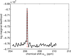
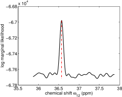
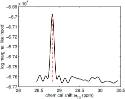
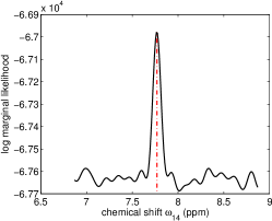
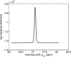
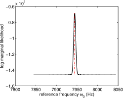
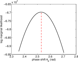
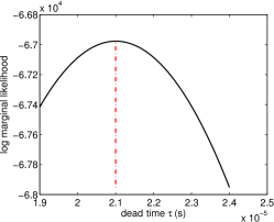
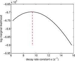
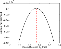
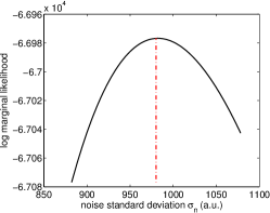
In Figure 3, we illustrate the behaviour of the marginal likelihood in Eq. (5.5) as a function of the nuisance parameters $\psi,v$, on a synthetic equal mixture of cyclohexane and 2-butanone. We generate the data by sampling from the generative model in Eqs. (3.3)–(3.4) with frequencies and intensities for cyclohexane and 2-butanone as given in Table 1.

Each panel in Figure 3 shows how the marginal likelihood varies as a function of a single parameter in the model of Eq. (3.1), with all other parameters set to the true generating values. The true values are shown with dashed vertical lines. Even in simulation, the likelihood surface is severely multimodal as a function of the frequency parameters. Moreover, there are strong dependencies between the frequency and phase parameters. Therefore exploring this likelihood surface is non-trivial. Our prior knowledge of the frequencies is only accurate to within about $1000$ rad/s (or $2$ ppm). We can see in Figure 3–3 that this range spans multiple local optima. A naive gradient based optimizer – greedily choosing to improve the value of an objective function on every iteration – will converge to undesirable local optima, rendering predictions of the amplitudes unusable. Likewise, popular sampling schemes, such as Metropolis Hastings, become stuck in a local optimum if using a small step size, and proposals with a large step size are rejected. We can also see that sampling may have limited value in this application, since the global optima in the frequency space are sharply peaked. Moreover, while the posterior over the amplitude parameters is sensitive to the estimated values of the frequency parameters, this posterior is not so sensitive to noise variance or decay that exploring the unimodal distributions shown in Figure 3 would provide major performance gains.

The local optima arise because a signal composed of a sum of frequency components can be extremely well modelled in parts, while missing the rest of the signal entirely, by a range of erroneous frequencies. The smaller the signal, the less pronounced the multimodality. Increasing an estimate on the initial decay rate $\alpha$ decreases the amount of available information (since the signal is then assumed to decay away quickly), and therefore decreases the multimodality in the likelihood. Thus increasing the estimate of $\alpha$ has an annealing effect on the likelihood surface. Increasing the noise variance has a similar effect: the more noise, the less available signal. Indeed there are natural dependencies between the decay rate and noise variance parameters. An overly high decay rate means a large portion of the signal can only be explained as noise. In short, systematically overestimating the decay rate, as part of a gradient based optimization procedure, can be used to help locate a global optimum. However, we find an explicit simulated annealing simplex algorithm (SIMPSA) (Cardoso, Salcedo and Feyo de Azevedo, 1996; Nelder and Mead, 1965), which was especially designed for continuous, bounded, global optimization, more reliable for this NMR spectroscopy application.

In short, to estimate relative chemical concentrations, we follow a three step procedure:

1. Use SIMPSA to find the $\psi_{\text{est}},v_{\text{est}}$ that optimize the marginal likelihood $\log p(\bm{y}_{1},\bm{y}_{2}|\psi,v)$ in Equation (5.5), using a vague uninformative prior $p(\bm{a})$ on the amplitudes.

2. Analytically infer the posterior $p(\bm{a}|\bm{y}_{1},\bm{y}_{2},\psi_{\text{est}},v_{\text{est}})$ as in Equation (4.1), conditioned on the maximum marginal likelihood estimates of the nuisance parameters $\psi,v$.

3. By sampling from $p(\bm{a}|\bm{y}_{1},\bm{y}_{2},\psi_{\text{est}},v_{\text{est}})$, sample from the distribution over the relative concentrations $r_{ij}=|A_{i}/A_{j}|$ of chemicals $i$ and $j$, $p(r_{ij}|\bm{y}_{1},\bm{y}_{2},\psi_{\text{est}},v_{\text{est}})$, where $A_{i}$ is the $i^{\text{th}}$ component of $\bm{a}$.

The computational demands of the proposed procedure are dominated by the need to evaluate the marginal likelihood of Eq. (5.5) for a variety of settings of $\psi$ and $v$. Each such evaluation costs $\mathcal{O}((N+M)r^{2}+r^{3})$ operations for $N$ and $M$ points respectively in the real and imaginary channels, and $r$ chemical species: it takes $(N+M)r^{2}$ operations to compute $\Phi^{\top}\Phi+\Psi^{\top}\Psi$, and $\mathcal{O}(r^{3})$ operations to take the Cholesky decomposition of this term (for solving linear systems). Thus for a system with a fixed number of chemicals, the required computational operations scale linearly with the number of collected datapoints.

6 Related Work

There is a body of groundbreaking work using models motivated for NMR spectroscopy, similar in form to Equation (3.1). In this section we briefly describe a selection of this work, and some limitations. Yoon et al. (2006) provide a general review of statistical models with various NMR applications.

Bretthorst (1990) was an early pioneer of Bayesian estimation of a quadrature model, similar to Eq. (3.1), but without the local phase shift $\tau$. While inference over the amplitude variables follows a similar procedure to that described in section 4, inference over the frequency variables involves several approximations, including a quadratic Taylor series expansion, leading to a Gaussian posterior over frequencies. However, in general, the posterior over frequencies can be highly non-Gaussian (as shown in Figure 3). Generally, these approximations are not robust to a multimodal likelihood surface, and tend to break down when there are more than a few resonant frequencies to estimate. Evilia, Effiong and Whittenburg (1993) contains a similar early quadrature NMR model, but the exact model specification and estimation procedures are unclear, and the model is tested on systems with at most 2 resonant frequencies.

Andrec and Prestegard (1998) use Metropolis Hastings to sample from the posterior distribution over parameters in a quadrature model similar to Bretthorst (1990), ultimately to estimate coupling constants in antiphase doublets. Andrec and Prestegard (1998) do not estimate more than two frequency parameters at a time, and do not compare with conventional spectroscopy. Furthermore, Metropolis Hastings (MH) is not generally suitable for exploring multimodal likelihood surfaces, as discussed in section 5. In short, using an MH proposal distribution with a small width will cause the sampler to become trapped in undesirable local optima, while a large width proposal is extremely unlikely to find a global optimum, and if it does, it will never move from a point estimate, which defeats the purpose of sampling.

Dou and Hodgson (1995) perform Gibbs sampling (Geman and Geman, 1984) for parameter estimation, with similar performance to Bretthorst (1990). Gibbs sampling involves alternately sampling one parameter while conditioning on the others, in a cycle. When there are strong dependencies between parameters, such as frequency and phase parameters, and multimodality, Gibbs sampling is known to mix poorly (murray-adams-2010a). Therefore a Gibbs sampling procedure may struggle in many NMR applications.

Rubtsov and Griffin (2007) focus on estimating the number of components (e.g., resonant frequencies) in a model similar to Bretthorst (1990), using reversible jump Markov chain Monte Carlo (MCMC). While the model is applied to experimentally acquired data, the experiments are taken in the ${}^{1}\text{H}$ spectrum, where the signal to noise ratio is much higher than in the ${}^{13}\text{C}$ spectrum.

In recent work, Hutton et al. (2009) develop a specialised model for mixtures of water and metabolites. The model has a similar form to Bretthorst (1990), except the amplitude coefficient for water is time-varying. Estimation of frequency parameters follows a simulated annealing MCMC approach. It is difficult to determine whether the methodology in Hutton et al. (2009) is generally applicable to quadrature NMR models, since the paper is focused on a specialised application in the (¹H) proton spectrum, where the SNR is much higher than in the carbon spectrum (considered in our paper), there is no comparison to conventional spectroscopy, and there is no motivation or description of the applied sampling scheme, except that the computational costs can be considerable.

Rather than construct a model in the time domain, Astle et al. (2012) consider modelling preprocessed data (apodised, phase corrected, and with a baseline correction) in the frequency domain, leveraging positivity requirements in this domain. While promising, the model relies on conventional preprocessing and implicit assumptions of the discrete Fourier transform (DFT), and thus may not be as general as time domain models.

Furthermore, Rubtsov et al. (2010) develop a promising statistical procedure for estimating resonant frequencies in the ${}^{1}\text{H}$ spectrum, independently from quadrature NMR models, and compare to binning. And Aboutanios, Kopsinis and Rubtsov (2012) develop heuristics for estimating components in a quadrature NMR model, which show some robustness to synthetic noise; however, the dataset considered is synthetic and has a well defined discrete Fourier transform.

Our paper focuses on aspects of quadrature NMR modelling which have not been thoroughly explored in prior work: 1) we develop a statistical model for NMR spectroscopy with a novel chemical quantification application, 2) we discuss challenges in estimating quadrature NMR models, such as a multimodality, and propose solutions, 3) we provide thorough quantitative comparisons with conventional Fourier transform spectroscopy, and 4) we consider both synthetic and experimentally acquired data in the ¹³C spectrum, with low SNR, and many resonant frequencies.

7 Simulations: 2-Butanone Cyclohexane Mixture

To better understand the behaviour of the proposed model (sections 3-5), and conventional Fourier transform (FT) spectroscopy (section 2), we first predict the relative concentrations of 2-butanone and cyclohexane in mixtures from synthetic free induction decay (FID) signals – a controlled environment with a ground truth. We simulate FID signals using the generative model of Equation (3.1), using the theoretical intensities from Table 1. Note that in real experiments, resonant frequencies will shift depending on the composition of a mixture, especially in the presence of commonly used solvents such as CDCl₃. Thus to make the simulations more representative of real experiments, and more challenging, we let the ground truth frequencies differ from the tabulated values by $\pm 3$ ppm, and initialise the estimation procedure of section 5 using the values in Table 1.

As can be seen in Figure 2, a synthetic FID from Eq. (3.1) resembles an actual FID response to a 2-butanone cyclohexane mixture. In section 8 we then compare these models on experimentally acquired FID signals.

7.1 Stress Tests

We start by stress testing the proposed model in response to varying signal to noise ratios (SNR) (as defined in Eq. (2.5)) in the FID signal.

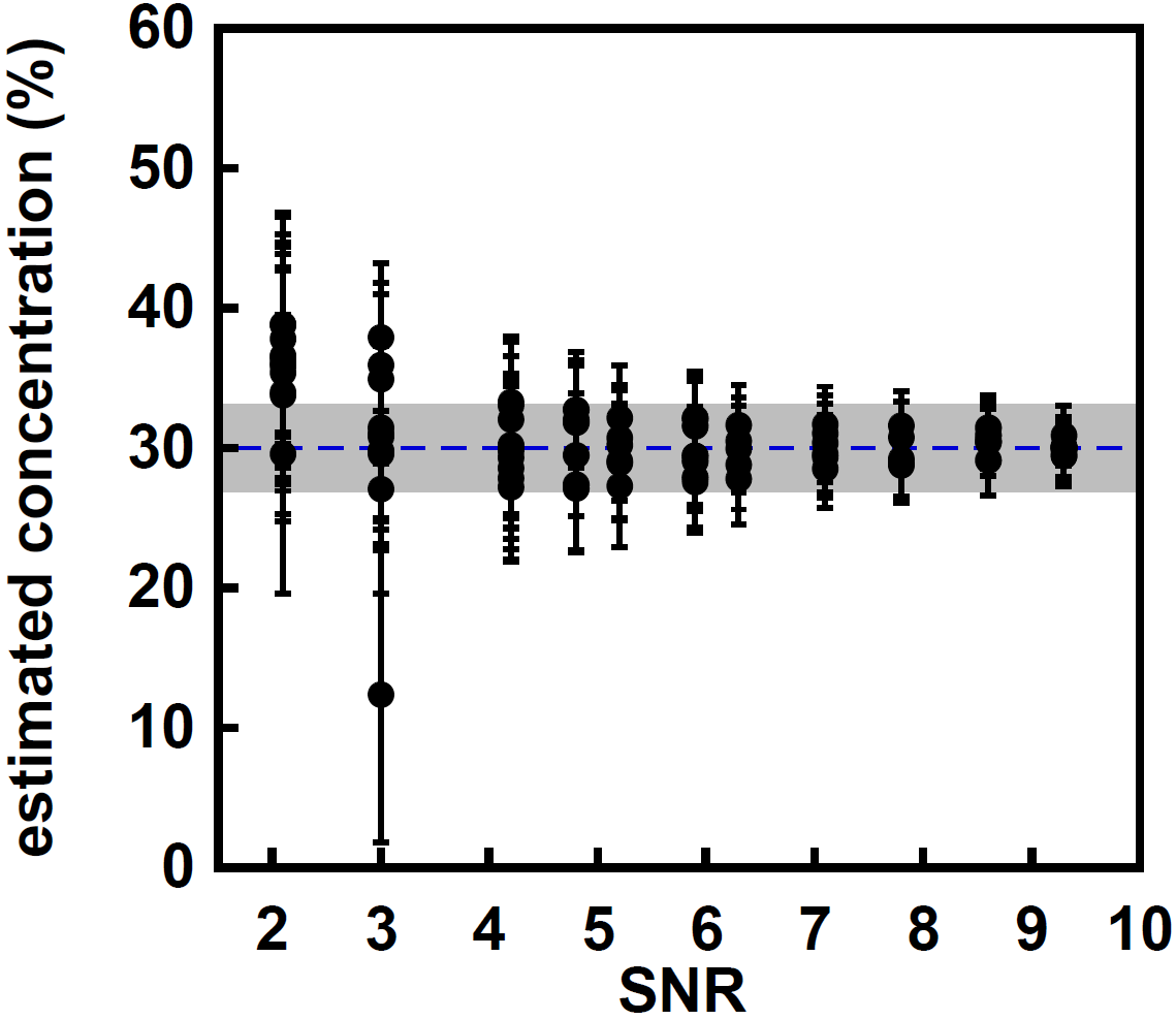
Taking a mixture of $30\%$ 2-butanone $70\%$ cyclohexane as an example, estimates and uncertainties regarding the concentration of 2-butanone, using the proposed model, are shown in Figure 4, with the true concentration of 2-butanone (30%) given by the dashed line. The gray shade indicates a concentration between 27%–33%. The error bars indicate a $95\%$ credible interval (two sample standard deviations of $p(|A_{i}/A_{j}||\bm{y}_{1},\bm{y}_{2},\psi,v)$ using $10000$ samples and the proposed model of section 3).

To test the robustness of the proposed model to noise, we selected a set of SNR values, and generated data 30 times for each of these values. As shown in Figure 4, above a SNR of $4$, the estimated concentrations are located within the gray shade (27%–33% 2-butanone), and contain the true concentration (30%) in 29/30 experiments. As expected, the estimated concentrations decrease in variance across different datasets as SNR increases, and converge to the true generating values. Figure 4 also shows that below an SNR of around $4$, the proposed model tends to overestimate the concentration of 2-butanone.

Figure 4: The relative concentration (and uncertainty) of 2-butanone in synthetic cyclohexane 2-butanone mixtures at various SNR, using the proposed model. The true concentration (30%) is given by the dashed line, with the shaded area representing 27%–33% 2-butanone. The error bars respresent the $95\%$ credible region.

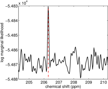
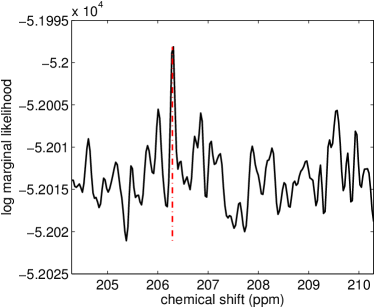
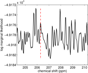
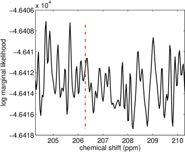
We now analyse the effect of increased noise on the marginal likelihood of the data, while keeping all other parameters fixed. Since the four resonant frequencies of 2-butanone behave similarly, we analyse the frequency near $206.29$ ppm.

Figure 5 displays the log marginal likelihood as a function of the frequency. The SNR gradually decreases from 5 to 5, with $5.9$ for 5, $4.2$ for 5, $3.0$ for 5, and $2.1$ for 5. As shown in Figure 5, the true frequency (indicated by the dashed line) becomes less differentiated as the SNR decreases, and the likelihood surface becomes increasingly multimodal, with no global optimum near the true generating frequencies. The precision of estimating the frequencies as well as the final concentrations at selected SNR were analysed by 30 repetitions and are given in Table 2.

In Figure 5 the true frequency is well-resolved, and indeed the proposed approach estimates the frequencies accurately, as given in Table 2. As the SNR decreases to $4.2$ (Figure 5), the marginal likelihood profile becomes less peaked at the true frequency. At such an SNR, the credible sets for the proposed method become relatively large, as shown in Table 2, and the method is more susceptible to the local optima shown in the likelihood surface of Figure 3. At this SNR level, the issue of local optima is largely alleviated with multiple SIMPSA restarts.

Figure 5: Log marginal likelihood plots as a function of a resonant frequency for butanone, with the true frequency ($206.29$ ppm) indicated by the dashed line. The corresponding SNR for each panel are 5 $5.9$, 5 $4.2$, 5 $3.0$, and 5 $2.1$. For high SNR values, 5 and 5, the peak at the true frequency is clearly identifiable.

Table 2: Bayesian estimates of the 2-butanone ($30\%$) and cyclohexane ($70\%$) mixture.

SNR	Error in frequency estimation (ppm) (mean $\pm 1$ std. dev.)	Bayesian $95\%$ credible interval	Empirical Coverage with $68\%$ and $(95\%)$ credible intervals	Percentage of reconstructions within 27%-33% 2-butanone
$9.3$	$-0.0039\pm 0.0096$	$1.09\%$	$91\%$ $(100\%)$	$100\%$
$5.9$	$-0.0072\pm 0.0043$	$3.44\%$	$50\%$ $(100\%)$	$100\%$
$4.2$	$-0.0067\pm 0.0187$	$4.92\%$	$82\%$ $(100\%)$	$82\%$
$3.0$	$0.3383\pm 0.7159$	$6.80\%$	$64\%$ $(73\%)$	$60\%$
$2.1$	$0.5608\pm 1.6385$	$8.34\%$	$27\%$ $(82\%)$	$9\%$

Figures 5 and 5 show the marginal likelihood at SNR values of $3.0$ and $2.1$ respectively. As the SNR increases, predictions with the proposed Bayesian model becomes increasingly accurate, converging to the truth, as shown in the second and last column in Table 2. When the SNR is above $4.2$, the proposed Bayesian method’s $95\%$ posterior credible interval always contains the true concentration.

7.2 Simulated Comparison to Conventional Spectroscopy: High Concentrations

We now examine the behaviour of both models in predicting high concentrations of a given chemical.

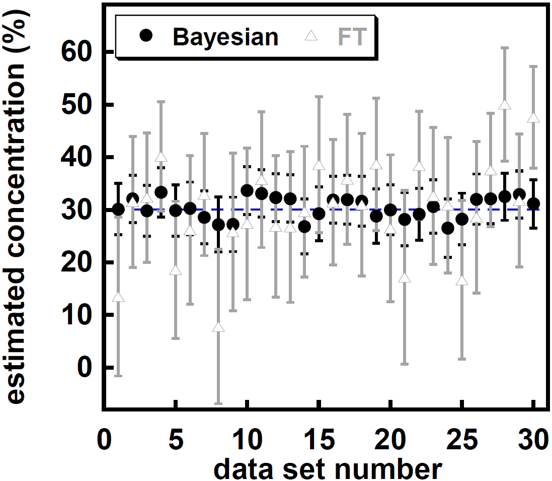
Results on a sample of $30\%$ 2-butanone at an SNR of $4.2$ are shown in Figure 6, with the true concentration indicated by the dashed line and the $95\%$ credible region given by the error bar. To confirm reproducibility, datasets were generated 30 times with the same concentration and SNR. Figure 6 shows that the proposed approach consistently makes accurate predictions that always include the true value in the 95% credible interval. Its estimates are always within a $30\%\pm 3.5\%$ bound.

Conversely, predictions using the conventional FT approach vary significantly in a $\pm 20\%$ concentration interval, and even with broader error bars than the proposed approach FT estimates are typically unable to cover the true concentration. The FT approach is particularly sensitive to noise, which will become even more apparent when we study low concentrations.

Figure 6: Comparison of the Bayesian and FT performances on the same FID datasets. 30 repetitions are generated for 30% 2-butanone at an SNR of $4.2$. The dashed line indicates the true concentration and the error bars correspond to $95\%$ credible regions.

We perform a similar analysis for 2-butanone concentrations ranging from $10\%$ to $90\%$. For clarity, representative results from only two datasets at each concentration were plotted in Figure 7, with the same noise level.

The Bayesian uncertainty intervals generally decrease as the concentration of 2-butanone rises from $10\%$ to $90\%$. Notice in Table 1 that cyclohexane has a single intensity near $6$, whereas 2-butanone has 4 intensities near $1$. Due to the lower intensities of 2-butanone, relative to cyclohexane, it is more difficult to differentiate the signal from $2$-butanone from the noise, and so predictions of both cyclohexane and butanone concentrations ought to be more accurate and certain as the relative concentration of $2$-butanone rises. Similarly, uncertainty in the FT predictions of cyclohexane increase with relative increases in cyclohexane concentrations (decreases in 2-butanone).

Figure 7: The proposed Bayesian and conventional FT estimations for varying relative concentrations of 2-butanone and cyclohexane in simulation. The noise levels for all the data are the same and are chosen to allow the SNR to be as low as possible but still retain acceptable performance. In particular, the SNR is $4.5$ for the mixture containing $10\%$ 2-butanone. The vertical axis shows absolute errors. The proposed Bayesian approach is more accurate and robust than the conventional FT approach in terms of both expected mean and uncertainty.

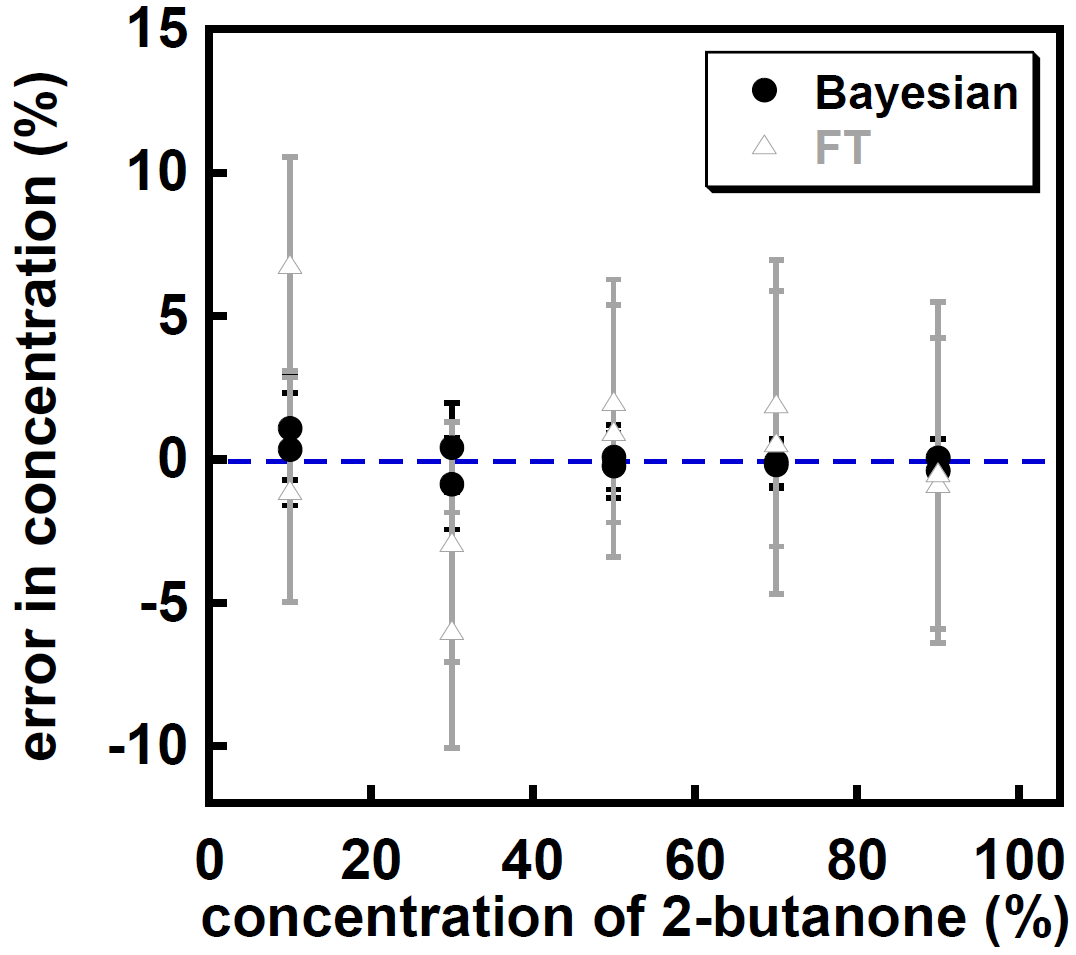
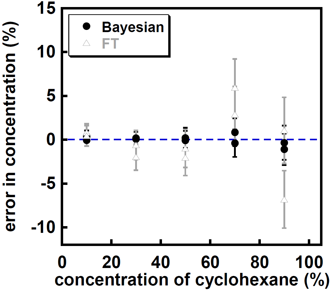
In the cases presented, the proposed Bayesian approach consistently produces more accurate point predictions and smaller and more accurate uncertainty intervals than a conventional Fourier transform approach.

7.3 Simulated Comparison to Conventional Spectroscopy: Low Concentrations

We now investigate the performance of the proposed Bayesian approach compared to the convential FT approach on low concentrations ($<10\%$). Low concentrations are of particular interest, as spectroscopers often wish to determine the presence or absence of a chemical in a system, or whether a particular chemical falls under a given concentration threshold. As we will see, the lower the concentration of a chemical, the harder the concentration is to accurately estimate.

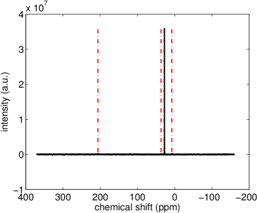
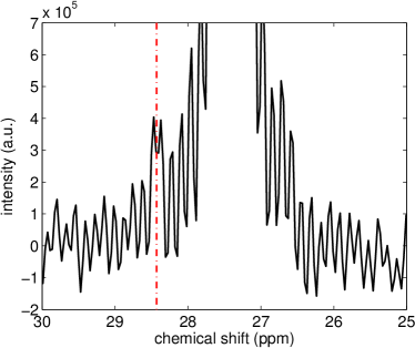
We begin with a simulation using $5\%$ 2-butanone with an SNR of $6$. Figure 8 shows the whole FT spectrum for this dataset, with the locations of expected peaks indicated by the dashed lines. It is very difficult to see the low intensity peaks from 2-butanone. Figure 8 zooms in to part of the spectrum indicated by the red box in 8. As shown in Figure 8, a peak from the dilute species, 2-butanone, overlaps with a high intensity peak from the concentrated species cyclohexane, which makes assignment of this peak difficult, causing the concentration of dilute chemicals to be overestimated. Moreover, the duration of the acquisition is limited owing to the radio frequency (rf) pulse used for proton decoupling (Keeler, 2011). This limited acquisition time causes truncation artifacts on the cyclohexane peak at $27.3$ ppm, making it more difficult to differentiate the butanone peak at $28.4$ ppm.

The Bayesian log marginal likelihood as a function of the same frequency from 2-butanone is displayed in Figure 8, with the same frequency window as used for the FT in 8.

As shown in Figure 8, using the proposed Bayesian method, true resonant frequencies of dilute species are well-resolved even in the presence of a nearby intense peak, due to the principled models of decay and noise in the FID signal. Such log marginal likelihood shape reduces the difficulty of learning the right frequency in the Bayesian procedure and, as shown in Figure 8, the final probability distribution is well resolved with a $2.4\%$ relative error ($0.12\%$ absolute error).

Figure 8: Comparison between the proposed Bayesian model and conventional Fourier transform spectroscopy on the same synthetic FID dataset. The ground truth frequencies are $206.29,36.57,28.43,7.77$ ppm for butanone and $27.3$ ppm for cyclohexane. The data were generated assuming a mixture of $5$ percent 2-butanone with an SNR of $5.9$ 8 The whole FT spectrum. 8 Zoom in to part of the spectrum indicated by the red box in 8. The peak ($28.43$ ppm) from 2-butanone is on the shoulder of the peak ($27.3$ ppm) from cyclohexane, and is prone to overestimation owing to the truncation artifacts arising from that peak. 8 Log marginal likelihood as a function of the $28.43$ ppm resonance frequency. It is well distinguished from adjacent frequencies. 8 the concentration distribution of 2-butanone estimated from the proposed Bayesian model. The dashed lines indicate the true values. As shown in 8 truncation artifacts do not interfere with the performance of the proposed Bayesian model.

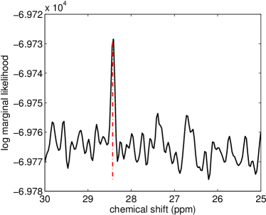
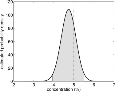
Simulated results for $3\%$ to $7\%$ 2-butanone are shown in Figure 9, with the true concentration given by the dashed line. The FT predictions are more variable than the Bayesian estimates, and systematically overestimate the concentration in almost all cases. Conversely, the Bayesian results have no noticable bias and the true concentrations are always within the credible region. The smaller error bar ($0.7\%$) – which has been reliable in these experiments – also allows the Bayesian approach to reliably distinguish between small concentration differences.

Figure 9: Simulated comparison of the Bayesian and FT approaches at low concentrations of 2-butanone. FID data were simulated with the a minimum noise level for acceptable performance (an SNR of $4.4$, which is the smallest SNR at which the $3\%$ concentration can be reasonably estimated). The true concentrations are given by the dashed line.

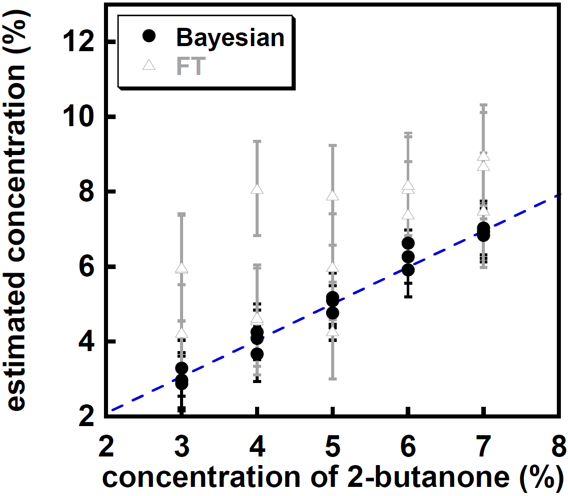
In conclusion, the analysis of the synthetic data at low concentrations ($<10\%$) demonstrates the strength of the Bayesian approach: it is more accurate than the FT, particularly in peak overlapping situations, or when the SNR or chemical concentration levels are particularly low.

8 Experiments

We now compare the proposed Bayesian model with a conventional spectroscopy approach on experimentally acquired FID signals corresponding to mixtures of cyclohexane and 2-butanone.

Cyclohexane ($\geq$ 99.5%) and 2-butanone ($\geq$ 99.5%) were purchased from Sigma Aldrich. The mixtures were prepared by mixing the two chemicals with various concentrations based on weight. To confirm reproducibility of results, each mixture was made twice and both preparations were used in the experiments. The error in sample preparations was calculated from the uncertainty in the electronic scale.

Conventional spectroscopy experiments were performed on a Bruker DMX300 spectrometer operating at a ¹³C resonance frequency of 75.47 MHz with a 5mm microimaging probe. The reference frequency $\omega_{0}$ was calibrated using the standard reference tetramethylsilane (TMS).

The default digital filter on the spectrometer performs an unknown transformation (for proprietary reasons) on the FID signal, making the generative model in Eq. (3.1) inapplicable. We therefore acquire the FID signal digitally, to minimise the noise in acquisition, and then use the TopSpin (Bruker) software on the spectrometer to convert the signal to a “pseudo-analogue” form. This approach maintains the integrity of the generative model in Eq. (3.1). We found the performance of the conventional Fourier transform method is equivalent using the digital or pseudo-analogue form of the FID signal.

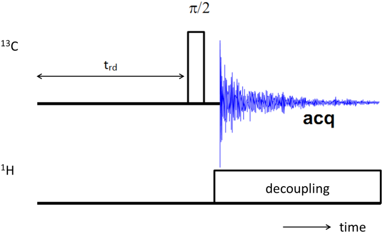
Experimentally, the time domain FID data were acquired using a single $90^{\circ}$ pulse on ¹³C channel with broadband ¹H decoupling, as shown in Figure 10. Each FID data set consists of $4096$ complex pairs with a $25\mu s$ sampling interval. The recycle time (the time between excitations of the system) was set as $180s$ to allow sufficient relaxation recovery. The digitally filtered FID data were converted to pseudo-analogue data format after acquisition using TopSpin software, which modified the number of data points to $4029$.

Phase correction was manually performed on the spectrometer using both zero and first order phase corrections ($\theta$ and $\tau$ in Eq. (3.1)) to ensure all peaks are in the so-called “absorption mode” (Keeler, 2011).

Figure 10: NMR on-pulse sequence.

Because the NMR spectrometer can only excite the spins within a certain resonance frequency range, the extent to which each chemical group is excited differs from each other slightly. To account for this behaviour, we adjust the intensities $B^{(k)}_{i}$ in the signal model of Eq. (3.1) as described in section 2 and Table 1.

8.1 Experimental Comparison to Conventional Spectroscopy: High Concentrations

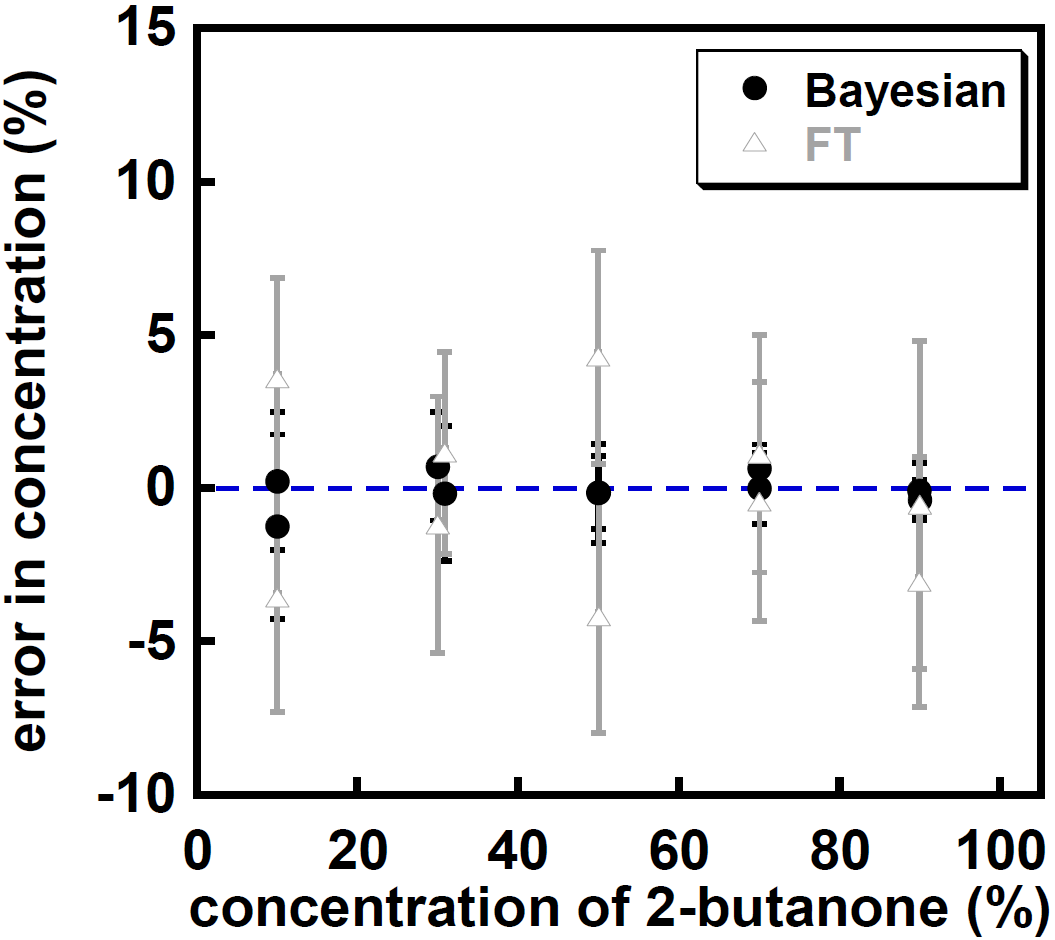
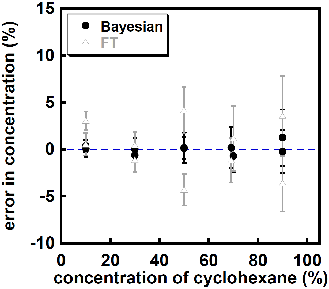
We first perform experimental measurements on mixtures of reasonably high concentrations, from $10\%$ to $90\%$. Similar to the simulations, the noise level was set by fixing the number of scans in experiments, with an SNR for the lowest concentration just above a threshold of 4.5, determined in section 7.2. To confirm the ground truth of the concentration, data were acquired from two prepared samples at each concentration. Estimation errors are shown in Figure 11. Similar accuracy and general behaviour as in the simulations (Figure 7) are observed. Accordingly, the proposed Bayesian approach has far less error and more realistic uncertainty estimates than the conventional Fourier transform approach.

Figure 11: Experimental results from Bayesian and FT approaches. The concentrations and SNR were set similar to the simulation cases shown in Figure 7. To avoid bias in the ground truth, data were acquired on two sets of samples. Error bars along the x axis were plotted but are too small to be seen.

8.2 Experimental Comparison to Conventional Spectroscopy: Low Concentrations

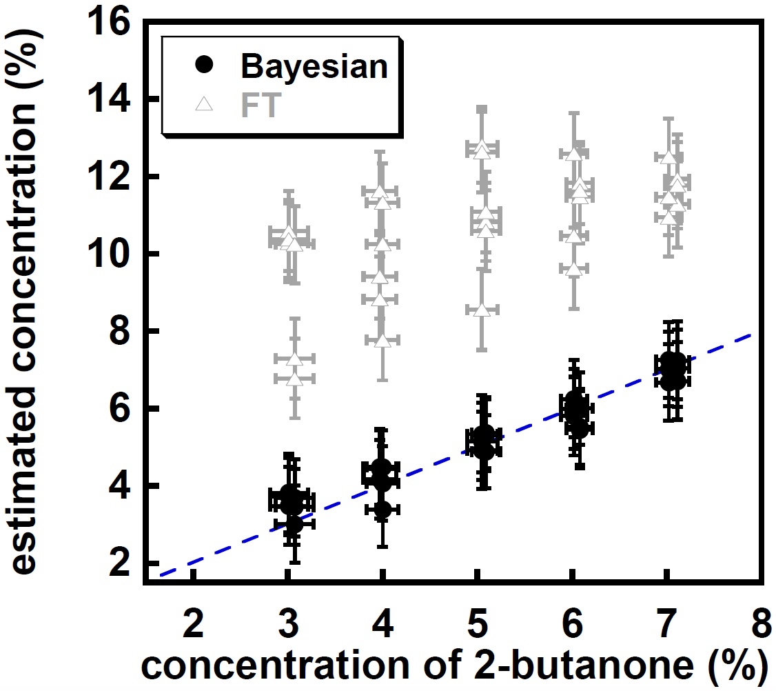
We now investigate experimentally the ability of the proposed method and conventional spectroscopy to estimate low concentration levels of 2-butanone. We prepare sets of samples with concentrations ranging from $3\%$ to $7\%$ in $1\%$ increments. We create two sets per concentration level and perform $3$ independent measurements on each sample. The SNR for the $3\%$ cases is 4.4. The Bayesian and FT results are shown in Figure 12, with the expected concentration (ground truth determined during mixture preparation) indicated by the dashed line. The error bars along the horizontal direction represent the error in sample preparation. The FT method consistently overestimates the concentration whereas there is no systematic bias from the Bayesian results. Moreover, the FT results from the same sample can scatter over a $5\%$ range and their error bars are unrealistically small. In contrast, the Bayesian predictions are always within a $1\%$ concentration bound and with more reliable uncertainty estimates.

Figure 12: Experimental comparison between the Bayesian model and FT for inferring low concentration levels. The data were acquired at the same noise level that allows the lowest concentration to be robustly estimated. Two samples were prepared at each concentration with three independent datasets acquired from each sample.

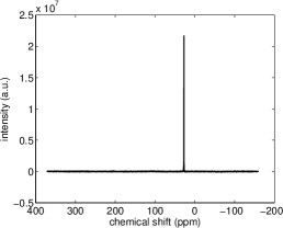
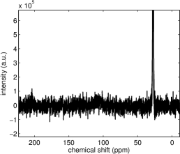
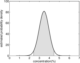
A particular set of data from the low concentration cases were taken to provide a more visual description. Figure 13 shows the results of a dataset from a $3\%$ 2-butanone mixture. The conventional FT spectrum, Figure 13, does not show the peaks from the $3\%$ 2-butanone. It is difficult to differentiate most of the peaks in 2-butanone, as shown in Figure 13. However, the proposed Bayesian approach can still infer the true concentration with reasonable accuracy and uncertainty.

Figure 13: Experimental findings on a $3.07\%\pm 0.20\%$ 2-butanone mixture. 13 Conventional Fourier spectrum. 13 Zoom in to the low intensity 2-butanone peaks. The peaks are almost at the same height as the noise level and cannot be assigned and quantified accurately. 13 Concentration probability distribution of 2-butanone calculated from the Bayesian model. The shaded area gives the $95\%$ credible region.

9 Discussion

We have proposed an alternative method for nuclear magnetic resonance spectroscopy. Unlike conventional Fourier transform spectroscopy, the proposed approach explicitly models decay, noise, frequencies, intensities, and phase shifts, and can leverage prior information in a principled way using probability distributions. We compared the proposed Bayesian approach with conventional Fourier transform spectroscopy in simulations and on experimentally acquired free induction decay signals, for quantifying relative chemical concentrations in a mixture. The proposed approach significantly outperformed conventional spectroscopy, with more accurate estimates and uncertainty intervals, particularly in low signal to noise ratio cases, and in cases where there were overlapping peaks in the Fourier transform of the free induction decay. In summary, the proposed method – while sensitive to frequency estimation – can be used with little human intervention, for reproducible and accurate estimates of chemical concentrations, and may be used in detecting the presence or absence of chemicals where conventional Fourier transform spectroscopy cannot be used. In general, the robustness of the proposed method to low signal to noise ratios, and overlapping spectral peaks, has widespread promise in analytic chemistry.

References

- Aboutanios, Kopsinis and Rubtsov (2012) {barticle}[author] \bauthor\bsnmAboutanios, \bfnmElias\binitsE., \bauthor\bsnmKopsinis, \bfnmYannis\binitsY. and \bauthor\bsnmRubtsov, \bfnmDenis\binitsD. (\byear2012). \btitleInstantaneous frequency based spectral analysis of nuclear magnetic resonance spectroscopy data. \bjournalComputers & Electrical Engineering \bvolume38 \bpages52–67. \endbibitem
- Andrec and Prestegard (1998) {barticle}[author] \bauthor\bsnmAndrec, \bfnmM.\binitsM. and \bauthor\bsnmPrestegard, \bfnmJ. H.\binitsJ. H. (\byear1998). \btitleA Metropolis Monte Carlo implementation of Bayesian time-domain parameter estimation: application to coupling constant estimation from antiphase multiplets. \bjournalJournal of Magnetic Resonance \bvolume130 \bpages217–232. \endbibitem
- Astle et al. (2012) {barticle}[author] \bauthor\bsnmAstle, \bfnmWilliam\binitsW., \bauthor\bsnmDe Iorio, \bfnmMaria\binitsM., \bauthor\bsnmRichardson, \bfnmSylvia\binitsS., \bauthor\bsnmStephens, \bfnmDavid\binitsD. and \bauthor\bsnmEbbels, \bfnmTimothy\binitsT. (\byear2012). \btitleA Bayesian model of NMR spectra for the deconvolution and quantification of metabolites in complex biological mixtures. \bjournalJournal of the American Statistical Association \bvolume107 \bpages1259–1271. \endbibitem
- Barrett et al. (2013) {barticle}[author] \bauthor\bsnmBarrett, \bfnmPaul J\binitsP. J., \bauthor\bsnmChen, \bfnmJiang\binitsJ., \bauthor\bsnmCho, \bfnmMin-Kyu\binitsM.-K., \bauthor\bsnmKim, \bfnmJi-Hun\binitsJ.-H., \bauthor\bsnmLu, \bfnmZhenwei\binitsZ., \bauthor\bsnmMathew, \bfnmSijo\binitsS., \bauthor\bsnmPeng, \bfnmDungeng\binitsD., \bauthor\bsnmSong, \bfnmYuanli\binitsY., \bauthor\bsnmVan Horn, \bfnmWade D\binitsW. D., \bauthor\bsnmZhuang, \bfnmTiandi\binitsT., \bauthor\bsnmSönnichsen, \bfnmFrank D\binitsF. D. and \bauthor\bsnmSanders, \bfnmCharles R\binitsC. R. (\byear2013). \btitleThe quiet renaissance of protein nuclear magnetic resonance. \bjournalBiochemistry \bvolume52 \bpages1303–20. \endbibitem
- Bloch, Hanson and Packard (1946) {barticle}[author] \bauthor\bsnmBloch, \bfnmF\binitsF., \bauthor\bsnmHanson, \bfnmW\binitsW. and \bauthor\bsnmPackard, \bfnmM\binitsM. (\byear1946). \btitleNuclear induction. \bjournalPhys Rev \bvolume69 \bpages127. \endbibitem
- Bretthorst (1990) {barticle}[author] \bauthor\bsnmBretthorst, \bfnmG. L.\binitsG. L. (\byear1990). \btitleBayesian analysis. I. Parameter estimation using quadrature NMR models. \bjournalJournal of Magnetic Resonance (1969) \bvolume88 \bpages533–551. \endbibitem
- Cardoso, Salcedo and Feyo de Azevedo (1996) {barticle}[author] \bauthor\bsnmCardoso, \bfnmM. F.\binitsM. F., \bauthor\bsnmSalcedo, \bfnmRL\binitsR. and \bauthor\bparticleFeyo de \bsnmAzevedo, \bfnmS.\binitsS. (\byear1996). \btitleThe simplex-simulated annealing approach to continuous non-linear optimization. \bjournalComputers & chemical engineering \bvolume20 \bpages1065–1080. \endbibitem
- Chen et al. (2005) {barticle}[author] \bauthor\bsnmChen, \bfnmQuan\binitsQ., \bauthor\bsnmMarble, \bfnmAndrew E\binitsA. E., \bauthor\bsnmColpitts, \bfnmBruce G\binitsB. G. and \bauthor\bsnmBalcom, \bfnmBruce J\binitsB. J. (\byear2005). \btitleThe internal magnetic field distribution, and single exponential magnetic resonance free induction decay, in rocks. \bjournalJournal of Magnetic Resonance \bvolume175 \bpages300–308. \endbibitem
- Dalitz et al. (2012) {barticle}[author] \bauthor\bsnmDalitz, \bfnmFranz\binitsF., \bauthor\bsnmCudaj, \bfnmMarkus\binitsM., \bauthor\bsnmMaiwald, \bfnmMichael\binitsM. and \bauthor\bsnmGuthausen, \bfnmGisela\binitsG. (\byear2012). \btitleProcess and reaction monitoring by low-field NMR spectroscopy. \bjournalProgress in nuclear magnetic resonance spectroscopy \bvolume60 \bpages52–70. \endbibitem
- Dou and Hodgson (1995) {barticle}[author] \bauthor\bsnmDou, \bfnmLixin\binitsL. and \bauthor\bsnmHodgson, \bfnmRJW\binitsR. (\byear1995). \btitleBayesian inference and Gibbs sampling in spectral analysis and parameter estimation. I. \bjournalInverse problems \bvolume11 \bpages1069. \endbibitem
- Ernst (1992) {barticle}[author] \bauthor\bsnmErnst, \bfnmRichard R\binitsR. R. (\byear1992). \btitleNuclear magnetic resonance Fourier transform spectroscopy. \bjournalBioscience reports \bvolume12 \bpages143–187. \endbibitem
- Evilia, Effiong and Whittenburg (1993) {barticle}[author] \bauthor\bsnmEvilia, \bfnmRonald F\binitsR. F., \bauthor\bsnmEffiong, \bfnmRosemary\binitsR. and \bauthor\bsnmWhittenburg, \bfnmScott L\binitsS. L. (\byear1993). \btitleBayesian estimation of NMR spectral parameters under low signal-to-noise conditions. \bjournalSpectroscopy letters \bvolume26 \bpages1559–1570. \endbibitem
- Geman and Geman (1984) {barticle}[author] \bauthor\bsnmGeman, \bfnmS.\binitsS. and \bauthor\bsnmGeman, \bfnmD\binitsD. (\byear1984). \btitleStochastic relaxation, Gibbs distributions, and the Bayesian restoration of images. \bjournalIEEE Transactions on Pattern Analysis and Machine Intelligence \bvolume6 \bpages721–741. \endbibitem
- Gladden (1994) {barticle}[author] \bauthor\bsnmGladden, \bfnmLF\binitsL. (\byear1994). \btitleNuclear magnetic resonance in chemical engineering: principles and applications. \bjournalChemical engineering science \bvolume49 \bpages3339–3408. \endbibitem
- Haacke et al. (1999) {bbook}[author] \bauthor\bsnmHaacke, \bfnmE Mark\binitsE. M., \bauthor\bsnmBrown, \bfnmRobert W\binitsR. W., \bauthor\bsnmThompson, \bfnmMichael R\binitsM. R. and \bauthor\bsnmVenkatesan, \bfnmRamesh\binitsR. (\byear1999). \btitleMagnetic resonance imaging: physical principles and sequence design \bvolume1. \bpublisherWiley-Liss New York. \endbibitem
- Hutton et al. (2009) {barticle}[author] \bauthor\bsnmHutton, \bfnmWilliam C\binitsW. C., \bauthor\bsnmBretthorst, \bfnmG Larry\binitsG. L., \bauthor\bsnmGarbow, \bfnmJoel R\binitsJ. R. and \bauthor\bsnmAckerman, \bfnmJoseph JH\binitsJ. J. (\byear2009). \btitleHigh dynamic-range magnetic resonance spectroscopy (MRS) time-domain signal analysis. \bjournalMagnetic Resonance in Medicine \bvolume62 \bpages1026–1035. \endbibitem
- Keeler (2011) {bbook}[author] \bauthor\bsnmKeeler, \bfnmJames\binitsJ. (\byear2011). \btitleUnderstanding NMR spectroscopy. \bpublisherWiley. \endbibitem
- Malz and Jancke (2005) {barticle}[author] \bauthor\bsnmMalz, \bfnmF\binitsF. and \bauthor\bsnmJancke, \bfnmH\binitsH. (\byear2005). \btitleValidation of quantitative NMR. \bjournalJournal of pharmaceutical and biomedical analysis \bvolume38 \bpages813–23. \endbibitem
- Nelder and Mead (1965) {barticle}[author] \bauthor\bsnmNelder, \bfnmJ. A.\binitsJ. A. and \bauthor\bsnmMead, \bfnmR.\binitsR. (\byear1965). \btitleA simplex method for function minimization. \bjournalThe computer journal \bvolume7 \bpages308–313. \endbibitem
- Purcell, Torrey and Pound (1946) {barticle}[author] \bauthor\bsnmPurcell, \bfnmEM\binitsE., \bauthor\bsnmTorrey, \bfnmHC\binitsH. and \bauthor\bsnmPound, \bfnmRV\binitsR. (\byear1946). \btitleResonance absorption by nuclear magnetic moments in a solid. \bjournalPhys Rev \bvolume69 \bpages37–38. \endbibitem
- Rabi et al. (1939) {barticle}[author] \bauthor\bsnmRabi, \bfnmII\binitsI., \bauthor\bsnmMillman, \bfnmS\binitsS., \bauthor\bsnmKusch, \bfnmP\binitsP. and \bauthor\bsnmZacharias, \bfnmJR\binitsJ. (\byear1939). \btitleThe Molecular Beam Resonance Method for Measuring Nuclear Magnetic Moments. The Magnetic Moments of _ 3 Li^6, _ 3 Li^7 and _ 9 F^19. \bjournalPhysical Review \bvolume55 \bpages526. \endbibitem
- Rasmussen and Ghahramani (2001) {binproceedings}[author] \bauthor\bsnmRasmussen, \bfnmCarl Edward\binitsC. E. and \bauthor\bsnmGhahramani, \bfnmZoubin\binitsZ. (\byear2001). \btitleOccam’s Razor. In \bbooktitleAdvances in Neural Information Processing Systems. \endbibitem
- Rubtsov and Griffin (2007) {barticle}[author] \bauthor\bsnmRubtsov, \bfnmDenis V\binitsD. V. and \bauthor\bsnmGriffin, \bfnmJulian L\binitsJ. L. (\byear2007). \btitleTime-domain Bayesian detection and estimation of noisy damped sinusoidal signals applied to NMR spectroscopy. \bjournalJournal of Magnetic Resonance \bvolume188 \bpages367–379. \endbibitem
- Rubtsov et al. (2010) {barticle}[author] \bauthor\bsnmRubtsov, \bfnmDenis V\binitsD. V., \bauthor\bsnmWaterman, \bfnmClaire\binitsC., \bauthor\bsnmCurrie, \bfnmRichard A\binitsR. A., \bauthor\bsnmWaterfield, \bfnmCatherine\binitsC., \bauthor\bsnmSalazar, \bfnmJosé Domingo\binitsJ. D., \bauthor\bsnmWright, \bfnmJayne\binitsJ. and \bauthor\bsnmGriffin, \bfnmJulian L\binitsJ. L. (\byear2010). \btitleApplication of a bayesian deconvolution approach for high-resolution 1h nmr spectra to assessing the metabolic effects of acute phenobarbital exposure in liver tissue. \bjournalAnalytical chemistry \bvolume82 \bpages4479–4485. \endbibitem
- Yoon et al. (2006) {barticle}[author] \bauthor\bsnmYoon, \bfnmJi Won\binitsJ. W., \bauthor\bsnmGodsill, \bfnmSimon\binitsS., \bauthor\bsnmKupče, \bfnmEriks\binitsE. and \bauthor\bsnmFreeman, \bfnmRay\binitsR. (\byear2006). \btitleDeterministic and statistical methods for reconstructing multidimensional NMR spectra. \bjournalMagnetic Resonance in Chemistry \bvolume44 \bpages197–209. \endbibitem