A New Approach to Tests and Confidence Bands for Distribution Functions
Abstract
We introduce new goodness-of-fit tests and corresponding confidence bands for distribution functions. They are inspired by multi-scale methods of testing and based on refined laws of the iterated logarithm for the normalized uniform empirical process and its natural limiting process, the normalized Brownian bridge process . The new tests and confidence bands refine the procedures of Berk and Jones (1979) and Owen (1995). Roughly speaking, the high power and accuracy of the latter methods in the tail regions of distributions are essentially preserved while gaining considerably in the central region. The goodness-of-fit tests perform well in signal detection problems involving sparsity, as in Ingster (1997), Donoho and Jin (2004) and Jager and Wellner (2007), but also under contiguous alternatives. Our analysis of the confidence bands sheds new light on the influence of the underlying -divergences.
AMS subject classifications.
60E10, 60F10 (primary); 62D99 (secondary).
Key words.
Confidence band, goodness-of-fit, law of the iterated logarithm, limit distribution, multi-scale test statistics
1 Introduction and motivations
1.1 Some well-known facts
Let be the empirical distribution function of independent random variables with unknown distribution function on the real line. The main topic of the present paper is to construct a confidence band for with given confidence level . That is, and are data-driven functions on the real line such that for any true distribution function ,
| (1.1) |
Let us recall some well-known facts about (cf. Shorack and Wellner (1986, 2009)). The stochastic process has the same distribution as , where is the empirical distribution of independent random variables with uniform distribution on . This enables the well-known Kolmogorov–Smirnov confidence bands: let
and let be the -quantile of the supremum norm . Then the confidence band with and satisfies (1.1) with equality if is continuous. Since converges in distribution in to standard Brownian bridge , converges to the -quantile of . In particular, the width of the Kolmogorov–Smirnov band is bounded uniformly by . (Throughout this paper, asymptotic statements refer to , unless stated otherwise.) On the other hand, it is well-known that Kolmogorov-Smirnov confidence bands give little or no information in the tails of the distribution ; see e.g. Milbrodt and Strasser (1990), Janssen (1995), and Lehmann and Romano (2005), chapter 14, for a useful summary.
1.2 Confidence bands by inversion of tests
In general, confidence bands can be obtained by inverting goodness-of-fit tests. For a given continuous distribution function , let be some test statistic for the null hypothesis that . Suppose that for any test level , the -quantile of under the null hypothesis does not depend on . Then a -confidence band for a continuous distribution function is given by
Depending on the specific choice of , these functions and can be computed explicitly, and the constraint (1.1) is even satisfied for arbitrary, possibly noncontinuous distribution functions ; see Section S.6 for further details.
Since corresponds to , one possibility to enhance precision in the tails is to consider weighted supremum norms such as
| (1.2) |
or
| (1.3) |
where are the order statistics of . Here, is some continuous weight function such that for and as . Specific proposals include
where , see Jaeschke (1979) and Eicker (1979), or sufficiently fast as , see O’Reilly (1974) or Csörgő et al. (1986). Specifically, Stepanova and Pavlenko Stepanova and Pavlenko (2018) propose to construct confidence bands with the test statistic (1.3) and . The latter choice is motivated by the law of the iterated logarithm (LIL) for the Brownian bridge process , stating that
| (1.4) |
almost surely.
1.3 The tests of Berk and Jones and Owen’s bands
Another goodness-of-fit test, proposed by Berk and Jones Berk and Jones (1979), uses the test statistic
| (1.5) |
where
for and . Note that is the Kullback-Leibler divergence between the and distributions. Owen Owen (1995) proposed and analyzed confidence bands for based on this test statistic. As noted by Jager and Wellner (2007), the test statistic can be embedded into a general family of test statistics , . Let
| (1.6) |
with the following divergence function : for ,
| (1.7) |
(An alternative representation of is given in (3.17).) Moreover, for fixed and , the limit equals if and exists in otherwise. A detailed discussion of these divergences is given in Section S.3 of the online supplement. At present it suffices to note that for any fixed , is strictly convex in with unique minimum at and second derivative there. Interesting special cases are , and
Consequently, if , then the test statistic coincides with times the square of in (1.2), and equals times the square of (1.3). As shown by Jager and Wellner (2007), for any , the null distribution of has the same asymptotic behavior, and the corresponding -quantiles satisfy
| (1.8) |
From this one can deduce that the resulting confidence band for satisfies
where ; see Lemma S.12 in Section S.3. Hence the band is substantially more accurate than in the tail regions. But in the central region, i.e. when is bounded away from and , they are of width rather than .
1.4 Goals revisited
The goal of Berk and Jones Berk and Jones (1979) was to find goodness-of-fit tests with optimal Bahadur efficiencies. They interpret their test statistic also as a union-intersection test statistic, where is the negative likelihood ratio statistic for the null hypothesis that , based on the binomial distribution of . The union-intersection and related paradigms for the present goodness-of-fit testing problem have been treated in more generality by Gontscharuk et al. (2016).
In view of the previous considerations, the confidence band of Stepanova and Pavlenko (2018), based on the test statistic
| (1.9) |
with , provides a trade-off between tail behavior and behavior in the center of the distribution. Previous proposals for the same purpose include Mason and Schuenemeyer (1983) and Révész (1982/83). But we shall demonstrate later that with purely multiplicative correction factors as in (1.9), the tail regions are asymptotically underemphasized in comparison with the new methods presented here.
1.5 Our new test statistics and confidence bands
To obtain a better compromise between the Kolmogorov–Smirnov and Berk–Jones tests, we propose a refined adjustment of involving a pointwise standardization together with a pointwise additive correction, where the latter takes into account whether is in the center or in the tails of or . Only after standardization and additive correction, we take a supremum over . This approach of pointwise standardization plus additive correction before taking a supremum has been developed in the context of multi-scale testing and has proved quite successful there; see e.g. Dümbgen and Spokoiny (2001), Dümbgen and Walther (2008), Schmidt-Hieber et al. (2013) and Rohde and Dümbgen (2013). In the present setting, pointwise standardization means that we consider , which behaves asymptotically like under the null hypothesis, that is, a squared standard Gaussian random variable times . To identify an appropriate additive correction term, we utilize a refinement of the LIL (1.4), based on Kolmogorov’s upper class test (cf. Erdös (1942), or Itô and McKean (1974), Chapter 1.8). For define
Then for any fixed ,
| (1.10) |
almost surely, where . Note that , , and, as ,
This indicates why (1.10) follows from Kolmogorov’s test (see Section S.1), and shows the connection between (1.10) and (1.4). On , both functions and are decreasing with and
Consequently, we propose the following test statistics:
| (1.11) |
where for ,
with . As seen later, using this bivariate version instead of or has computational advantages and increases power. The additive correction term is large only if is far in the tails of and of .
The remainder of this paper is organized as follows.
- •
-
•
Section 3 discusses statistical implications of this finding. As explained in Section 3.1, goodness-of-fit tests based on have desirable asymptotic power. In particular, they are shown to attain a detection boundary of Ingster Ingster (1997) for Gaussian mixture models. Moreover, even under contiguous alternatives they have nontrivial asymptotic power, as opposed to goodness-of-fit tests based on in (1.6).
-
•
In Section 3.2, we analyze the confidence bands resulting from inversion of the tests . It will be shown that these bands have similar accuracy as those of Owen Owen (1995) and the bands based on in the tail regions while achieving the usual root- consistency everywhere. In addition, we compare our bands with the confidence bands of Stepanova and Pavlenko (2018), confirming our claim that a purely multiplicative adjustment of is necessarily suboptimal in the tail regions.
-
•
Our results for the confidence bands elucidate the impact of the parameter on these bands for large sample sizes. These considerations are based on new inequalities and expansions for the divergences which are of independent interest.
All proofs and auxiliary results are deferred to Sections 4, 5 and an online supplement. References to the latter start with ‘S.’ or ‘(S.’. Essential ingredients for the proofs in Section 4 are tools and techniques of Csörgő et al. Csörgő et al. (1986). A first version of this paper used a different, more self-contained approach which is probably of independent interest and outlined in Section S.2. This also includes an alternative proof of (1.10).
2 Limit distributions under the null hypothesis
Recall the uniform empirical process mentioned in the introduction. Under the null hypothesis that , the test statistic has the same distribution as
| (2.12) |
where are the order statistics of the uniform sample . In particular, the -quantile of under the null hypothesis coincides with the -quantile of . Here is our main result for and .
Theorem 2.1.
For all and ,
Moreover, for any fixed test level , where is the -quantile of .
A key step along the way to proving Theorem 2.1 will be to consider the case and prove the following theorem for the uniform empirical process , where denotes the distribution function of the uniform distribution on .
Theorem 2.2.
For all ,
Remark 2.3 (The impact of and the definition of ).
Note that the parameter could be an arbitrary real number. However, numerical experiments indicate that the convergence to the asymptotic distribution is very slow if, say, or . More precisely, Monte Carlo experiments show that for parameters , the test statistcs are mainly influenced by just a few very small or very large order statistics. Moreover, if , one should redefine as a supremum over rather than . As shown in our proof of Theorem 2.1, this modification does not alter the asymptotic distribution, but for realistic sample sizes , taking the supremum over the full set for small parameters leads to distributions which are mainly influenced by .
Tables S.1 and S.2 provide exact critical values for various sample sizes , , and .
Similar discrepancies between asymptotic theory and finite sample behaviour can be observed for the Berk-Jones quantiles if , see Tables S.3 and S.4.
3 Statistical implications
3.1 Goodness-of-fit tests
As explained in the introduction, we can reject the null hypothesis that is a given continuous distribution function at level if the test statistic , defined in (1.11), exceeds the -quantile of . The test statistics and can be represented as the maximum of at most terms: with , the statistic equals
if , and
if . The statistic can be represented analogously with in place of . These formulae follow from the fact that for fixed , the function is continuous on , increasing on and decreasing on . For is convex in with minimum at , see (S.12) in Section S.3, and is increasing in and decreasing in . If , these monotonicities are also true for , precisely,
while and .
3.1.1 Non-contiguous alternatives
Now suppose that the true distribution function of the observations is a continuous distribution function such that . A first question is: under what conditions on the sequence does our goodness-of-fit test have asymptotic power one for any fixed test level . Since , this goal is equivalent to
| (3.13) |
To verify this property, the following function plays a key role:
for with the conventions and for .
Theorem 3.1.
It follows immediately from this theorem that (3.13) is satisfied whenever for all sample sizes , where .
As a litmus test for our procedures and Theorem 3.1, we consider a testing problem studied in detail by Ingster (1997). The null hypothesis is given by , the standard Gaussian distribution function, whereas
for certain numbers and . By means of Theorem 3.1 one can derive the following result.
Corollary 3.2.
As explained by Ingster (1997), any goodness-of-fit test at fixed level has trivial asymptotic power whenever for some and with
Thus part (a) of the previous corollary shows that our new family of tests achieves this detection boundary, as do the goodness-of-fit tests of Donoho and Jin (2004), Jager and Wellner (2007) and Gontscharuk et al. (2016).
A connection between parts (a) and (b) of Corollary 3.2 can be seen as follows: let for some fixed , and for some . Then for some , and with , we may write .
3.1.2 Contiguous alternatives
Suppose that the distribution functions and have densities and , respectively, with respect to some continuous measure on such that for some function ,
| (3.15) |
Then it follows easily that , and
Furthermore, since , the Cauchy-Schwarz inequality yields that
| (3.16) |
Lemma 3.3 (Power of “tail-dominated” tests under contiguous alternatives).
Let be a sequence of tests with the following two properties:
(i) For a fixed level ,
(ii) For any fixed and , , there exists a test depending only on such that
Then under assumption (3.15),
Note that the Berk-Jones tests with satisfy the assumptions of Lemma 3.3, if tuned to have asymptotic level . For all of them involve a test statistic of the type
with a function such that under the null hypothesis,
but for any ,
Hence equals
with asymptotic probability one. Thus we may replace the test statistic with while keeping the critical value.
By way of contrast, the goodness-of-fit test based on has nontrivial asymptotic power in the present setting.
Theorem 3.4 (Power of new tests under contiguous alternatives).
In the setting (3.15), the test statistic converges in distribution to
In particular,
Concerning the impact of ,
3.2 Confidence bands
The confidence bands of Owen (1995), defined in terms of , may be generalized to arbitrary fixed , but we restrict our attention to , because for and a large range of sample sizes , the resulting bands would focus mainly on small regions in the tails and be rather wide elsewhere. With confidence we may claim that does not exceed the -quantile of . As explained in Section S.6, inverting the inequality for fixed with respect to reveals that for and ,
where are given by , and for ,
Thus, computing the confidence band boils down to determining the numbers and , .
Our new method is analogous: with confidence , for and , the value is contained in
where , and for ,
To understand the asymptotic performance of these confidence bands properly, we need auxiliary functions . Note first that for any , in (1.7) may be represented as
| (3.17) |
where
| (3.18) |
for , and equals . If and are close to , one may approximate by
The properties of are treated in Lemma S.13. In particular, it is shown that
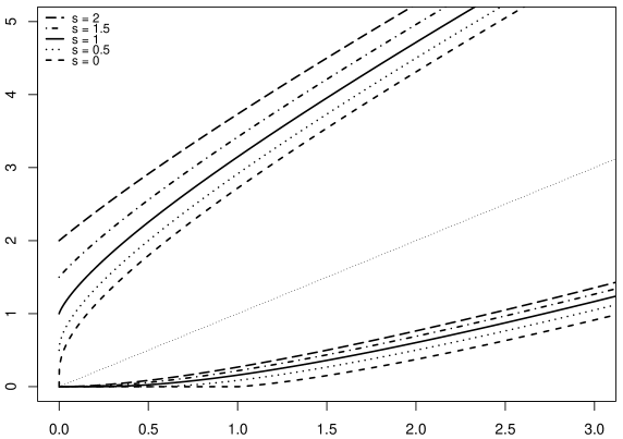
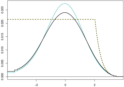
define continuous functions , where is convex with , if and only if , and is concave. Moreover, and as . Finally, for fixed , and are non-decreasing in with . Figure 1 depicts these functions on the interval for .
Our first result shows that the confidence bands and are asymptotically equivalent in the tail regions, that is, for close to zero or close to one. Moreover, the test level is asymptotically irrelevant there, but the parameter does play a role when .
Theorem 3.5.
Let . For any fixed , and ,
| and | ||||
uniformly in .
Remark 3.6 (Choice of ).
Concerning the choice of , Theorem 3.5 shows that smaller (resp. larger) values of lead to better upper (resp. lower) and worse lower (resp. upper) bounds for in the left tail and better lower (resp. upper) and worse upper (resp. lower bounds) for in the right tail. The choice seems to be a good compromise, see also the numerical examples later.
The next result shows that in the central region, the parameter is asymptotically irrelevant, and the width of the band is of smaller order than the width of .
Theorem 3.7.
For any fixed , and ,
uniformly in , where and .
Remark 3.8 (Comparison with Stepanova–Pavlenko Stepanova and Pavlenko (2018)).
The confidence band of Stepanova and Pavlenko (2018) with the test statistic in (1.9) can be represented as follows: for and ,
where , , , , and for ,
Recall that . Here is the -quantile of in case of , and it converges to the -quantile of
Consequently, for fixed , and ,
uniformly in . But
because and converge to as . Thus, the confidence band is asymptotically wider than in the tail regions for sufficiently small .
Note that these considerations apply to any choice of the continuous function in (1.9) as long as as .
Remark 3.9 (Bahadur and Savage Bahadur and Savage (1956) revisited).
On , the upper confidence bounds for are constant or , and this is of order . Likewise, on , the lower confidence bounds for are constant or . Interestingly, for any -confidence band for a continuous distribution function , the upper bound has to be greater than with asymptotic probability at least , and the lower bound has to be smaller than with asymptotic probability at least . This follows from a quantitative version of Theorem 2 of Bahadur and Savage (1956), stated as Theorem 3.10 below.
It is also instructive to consider Daniels’ lower confidence bound for a continuous distribution function , namely
Theorem 3.10.
Let be a family of continuous distribution functions which is convex and closed under translations, that is, for all and . Let be a -confidence band for . Then for any and ,
In our context, would be the family of all continuous distribution functions. But the precision bounds in Theorem 3.10 apply to much smaller families already, for instance, the family of all convex combinations of , , where is an arbitrary continuous distribution function. For the reader’s convenience, a proof of Theorem 3.10 is provided in Section S.5.
Example 3.11 ().
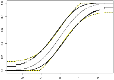
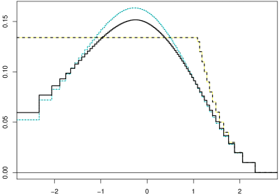
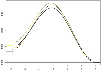
The left panel in Figure 2 depicts, for , the -confidence band in case of an idealized standard Gaussian sample with order statistics
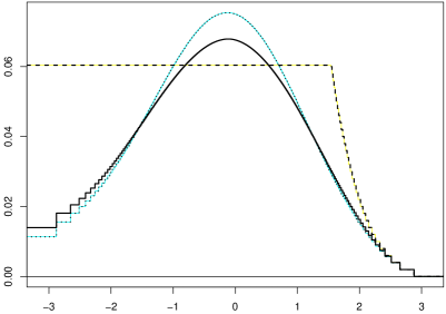
In addition, one sees the Kolmogorov–Smirnov -confidence band . In the right panel, one sees for the same setting the centered upper bounds , and . Note that a plot of the centered lower bounds , and would be the reflection of the plots for the centered upper bounds with respect to the point . The corresponding critical values , and have been computed numerically, see Section S.7.
Example 3.12 (The impact of ).
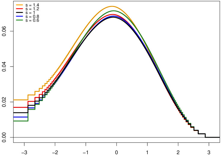
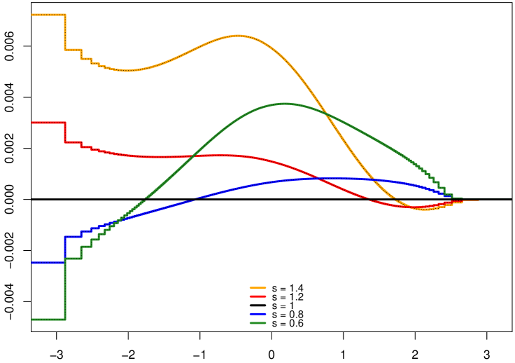
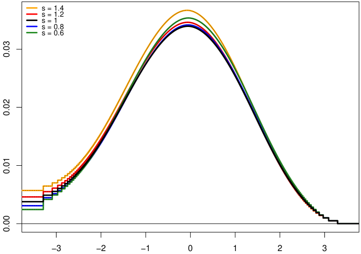
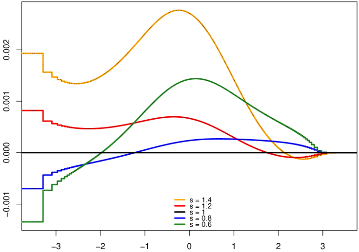
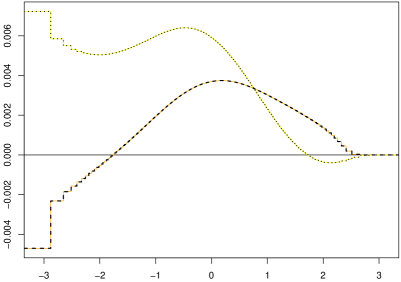
Figure 4 shows for an idealized Gaussian sample of size , the centered upper -confidence bounds for (left panel) as well as the differences for , right panel. As predicted by Theorem 3.5, the upper bounds are increasing in for small values of and decreasing in for large values of . The online supplement contains further plots illustrating the impact of on our bands. These plots support our claim that choosing close to is preferable. Other values of increase the bands’ precision somewhere in the tails, but lead to a substantial loss of precision in the central region.
Remark 3.13 (Discontinuous distribution functions).
In the previous considerations, we focused on continuous distribution functions , and all confidence bands for we considered are of the form
with certain numbers . Interestingly, such a band has coverage probability at least for arbitrary, not necessarily continuous distribution functions ; see Section S.6.
4 Proofs for Section 2
4.1 Proof of Theorem 2.2
The following three facts are our essential ingredients.
Fact 4.1 (Csörgő et al. (1986), Theorem 2.2 and Corollary 2.1).
There exist on a common probability space a sequence of i.i.d. random variables and a sequence of Brownian bridge processes such that, for all ,
Fact 4.2 (Csörgő et al. (1986), Theorem 4.4.1).
Fact 4.3 (Csörgő et al. (1986), Lemma 4.4.4).
For any such that and ,
The same holds with the supremum over .
Lemma 4.4.
For any sequence of constants such that and and any choice of ,
Lemma 4.5.
For all ,
The same holds with the supremum over replaced by .
Proof.
Lemma 4.6.
For any fixed ,
Proof.
Recall that
is finite almost surely for any . If we choose and write , then we see that for any ,
because is symmetric around and monotone decreasing on . Now the claim follows from almost surely and as . ∎
4.2 Proof of Theorem 2.1
Note first that in case of ,
because as and . Since , and ,
Consequently, it suffices to verify Theorem 2.1 with the modified test statistic
provided that we can show that the latter converges in distribution.
In what follows, we show that replacing with and with has no effect asymptotically. For these tasks, the following two facts are useful.
Fact 4.7 (Linear bounds for ).
Fact 4.8.
A particular consequence of Fact 4.7 is that
| (4.20) |
where , and Fact 4.8 implies that
| (4.21) |
with the conventions that and . This leads to the following useful bounds:
Lemma 4.9.
For any fixed ,
where . Moreover,
where in case of .
Proof.
Now the statement about the (modified) test statistic is an immediate consequence of Theorem 2.2 and the following lemma.
Lemma 4.10.
For and any ,
Proof.
It remains to prove the claim that . But this follows immediately from the following lemma.
Lemma 4.11.
Let . Then , and is continuous and strictly increasing on .
To prove this lemma and other results, we make use of the following well-known result.
Fact 4.12 (Borell (1974), Corollary 2.1; Gaenssler et al. (2007), Lemma 1.1).
The distribution of is a log-concave measure on . That means, for Borel sets and ,
where stands for the inner measure induced by , and .
From this fact one can deduce the following properties of :
Proposition 4.13.
For arbitrary functions and ,
is an even, log-concave function of . Furthermore, if , then
is a non-decreasing and log-concave function of .
Let be a standard Brownian motion process on . Then it is well-known that defines a Brownian bridge process on . The following self-similarity property of the Brownian bridge process seems to be less well-known.
Proposition 4.14.
For fixed numbers , define a stochastic process on as follows:
that is, describes the interpolation error when replacing on with its linear interpolation there. Then the two processes and are stochastically independent, and
Proof of Lemma 4.11.
Note first that the distribution function coincides with the function in Proposition 4.13, where and . In particular, , and the latter bound equals for and is strictly smaller than for any .
By Proposition 4.13, is log-concave, and since for all , this implies that is continuous and strictly increasing on , where . If we can show that , then we know that is, in fact, continuous and strictly increasing on .
To show that for any , we pick a number and write as the maximum of the three random variables
Then we can write
with .
According to Lemma 4.6, we may choose such that . Now we apply Proposition 4.14 twice, first with , and then with . This shows that may be rewritten on and on as follows: for ,
where are independent Brownian bridge processes. In particular,
where with and for . Analogously,
According to Proposition 4.13, is an even, log-concave function on . Since , there exists a such that for all . Consequently,
That for any follows, for instance, from the expansion
see Mogul’skiĭ (1979) or Shorack and Wellner (2009), pp. 526-527. Alternatively, one could use Proposition 4.13 and separability of . ∎
5 Proofs for Section 3
5.1 Proofs for Subsection 3.1
Proof of Theorem 3.1.
Let be a sequence in such that . Then for any fixed ,
| (5.22) | ||||
where if and .
To ensure that the first summand on the right hand side of (5.22) converges to , we show that may be chosen such that , where . To this end we have to analyze the auxiliary function in more detail. Elementary calculus reveals that for , is an increasing and is a decreasing function of . Moreover,
whence
In particular,
Now suppose that . With we may conclude that
In particular, is of order , so
Analogously one can show that in case of , we may replace with at the cost of reducing by a factor of at most .
It remains to show that
| (5.23) |
By means of the second part of Lemma S.12, the inequality for implies that
because , and for the univariate function , it follows from that . Moreover, the assumption that implies that
Consequently, (5.23) would be a consequence of
| (5.24) |
To bound the left-hand side of (5.24) we consider the quantity
and distinguish two cases. Suppose first that . Since
the definition of implies that
Then it follows from that
Now suppose that . Then,
with
Consequently,
∎
Proof of Corollary 3.2.
Since , it suffices to show that (3.14) is satisfied. In what follows we use frequently the elementary inequalities
| (5.25) |
where . In particular, as ,
Now consider two sequences and tending to , and let , . Then the inequalities (5.25) imply that
Moreover,
because while
Consequently, if
| (5.26) |
In part (a) with and , we imitate the arguments of Donoho and Jin (2004) and consider
with . Then by (5.25),
so the left hand side of (5.26) equals
The exponent in the enumerator is maximal in if , i.e. , and this leads to
Thus when we should choose and . When we should choose and .
As to part (b), we consider the more general setting that for some , where . Note that this scenario covers also a part of part (a), so we establish a connection between the two parts. The constraint that is trivial when but relevant when . Now we consider
with arbitrary constants . Now
so the left hand side of (5.26) equals
The exponent of becomes minimal in if . Then we obtain
and this converges to if the limiting exponents of and are negative. This is the case if . (Note that because .) ∎
Proof of Lemma 3.3.
Standard LAN theory implies that for arbitrary events depending on such that . Thus for any fixed , with asymptotic probability zero, both under the null and under the alternative hypothesis. Hence it suffices to show that
But does not change if we replace with the modified density
with
This follows from the fact that the distribution function of satisfies for , so the distribution of under the alternative hypothesis remains unchanged if we replace with . But
so
with
Hence the asymptotic power of the test under the alternative is bounded by the asymptotic power of the optimal test of versus at level , so
But
converges to as , so as . ∎
Proof of Theorem 3.4.
Let be fixed. The test statistic for the uniform empirical process may be written as the maximum of and , where
Here if and if . A supremum over the empty set is defined to be . The proofs of Theorems 2.2 and 2.1 can be easily adapted to show that
where the test statistics , and are defined as in the proof of Lemma 4.11. In particular, since and almost surely,
Note that as by virtue of Lemma 4.6.
Now we consider the goodness-of-fit test statistic . It is the maximum of and . Here is defined as , where is replaced with if and if , is replaced with , and is replaced with . Under the null hypothesis, has the same distribution as for . This convergence and standard LAN theory imply that under the alternative hypothesis,
With standard empirical process theory one can show that under the alternative hypothesis,
in the space of bounded functions on , equipped with the supremum norm . Moreover, for arbitrary bounded functions on such that ,
uniformly on . By virtue of an extended continuous mapping theorem, e.g. van der Vaart and Wellner (1996), Theorem 1.11.1, page 67, one can conclude that
where is defined as with in place of . Finally, note that the distribution of is absolutely continuous with respect to the distribution of , where has distribution under . This follows from Shorack and Wellner (2009) (Section 4.1 and especially Theorem 4.1.5, page 157), or van der Vaart and Wellner (1996) (Section 3.10). Consequently,
All in all, we may conclude that
and for fixed ,
Since as , this proves that converges in distribution to under the alternative hypothesis.
The convergence claimed in the second part of the theorem follows from the first part together with convergence of the critical values to . The inequality claimed in the second part is a consequence of Anderson’s Anderson (1955) inequality or Proposition 4.13 with and .
The third part of the theorem follows from the fact that for any ,
where is bounded on . ∎
5.2 Proofs for Subsection 3.2
For notational convenience, we suppress the dependence of the confidence bounds on , and and just write , , and .
Proof of Theorem 3.5.
Note first that for arbitrary , and .
Now we prove the claim for the upper bounds and . For any integer let
For fixed let
It follows from that
On the one hand, if , then it follows from the first inequality in (S.15) that
because is convex in with values for and for . And if , the second inequality in (S.15) implies that
On the other hand, and
Consequently, for any fixed and sufficiently large ,
and thus
for all integers . Likewise, for any fixed and sufficiently large ,
and thus
for all integers .
The differences and can be treated analogously. For each integer and fixed let as before and
On the one hand, if and , then and
because is convex in with values for and for . And if , then
On the other hand, and
Consequently, for any fixed and sufficiently large ,
for all integers . Likewise, for any fixed and sufficiently large ,
for all integers . ∎
Proof of Theorem 3.7.
We only prove the bounds for and . The bounds for and can be derived analogously with obvious modifications. Moreover, since , it suffices to prove the bounds for only. For a fixed factor and any integer let
Note that
whence
On the one hand, the inequalities (S.14) imply that uniformly in ,
On the other hand, Lemma S.10 and Theorem 2.1 imply that uniformly in ,
Consequently, for fixed and sufficiently large ,
and thus
for all integers . Likewise, for fixed and sufficiently large ,
and thus
for all integers . ∎
Acknowledgments.
The authors owe thanks to David Mason for pointing out the relevance of the tools of Csörgő et al. Csörgő et al. (1986) for some of the results presented here. We are also grateful to Günther Walther for stimulating conversations about likelihood ratio tests in nonparametric settings and to Rudy Beran for pointing out the interesting results of Bahadur and Savage Bahadur and Savage (1956). Constructive comments of two referees and an associate editor are gratefully acknowledged.
The first author was supported in part by the Swiss National Science Foundation.
The second author was supported in part by NSF Grant DMS-1104832 and NI-AID grant 2R01 AI291968-04.
References
- Alfers and Dinges (1984) Alfers, D. and Dinges, H. (1984). A normal approximation for beta and gamma tail probabilities. Z. Wahrsch. Verw. Gebiete 65 399–420.
- Anderson (1955) Anderson, T. W. (1955). The integral of a symmetric unimodal function over a symmetric convex set and some probability inequalities. Proc. Amer. Math. Soc. 6 170–176.
- Bahadur and Savage (1956) Bahadur, R. R. and Savage, L. J. (1956). The nonexistence of certain statistical procedures in nonparametric problems. Ann. Math. Statist. 27 1115–1122.
- Berk and Jones (1979) Berk, R. H. and Jones, D. H. (1979). Goodness-of-fit test statistics that dominate the Kolmogorov statistics. Z. Wahrsch. Verw. Gebiete 47 47–59.
- Borell (1974) Borell, C. (1974). Convex measures on locally convex spaces. Ark. Mat. 12 239–252.
- Csörgő et al. (1986) Csörgő, M., Csörgő, S., Horváth, L. and Mason, D. M. (1986). Weighted empirical and quantile processes. Ann. Probab. 14 31–85.
- Donoho and Jin (2004) Donoho, D. L. and Jin, J. (2004). Higher criticism for detecting sparse heterogeneous mixtures. Ann. Statist. 32 962–994.
- Dümbgen (1998) Dümbgen, L. (1998). New goodness-of-fit tests and their application to nonparametric confidence sets. Ann. Statist. 26 288–314.
- Dümbgen and Spokoiny (2001) Dümbgen, L. and Spokoiny, V. G. (2001). Multiscale testing of qualitative hypotheses. Ann. Statist. 29 124–152.
- Dümbgen and Walther (2008) Dümbgen, L. and Walther, G. (2008). Multiscale inference about a density. Ann. Statist. 36 1758–1785.
- Eicker (1979) Eicker, F. (1979). The asymptotic distribution of the suprema of the standardized empirical processes. Ann. Statist. 7 116–138.
- Erdös (1942) Erdös, P. (1942). On the law of the iterated logarithm. Ann. of Math. (2) 43 419–436.
- Gaenssler et al. (2007) Gaenssler, P., Molnár, P. and Rost, D. (2007). On continuity and strict increase of the CDF for the sup-functional of a Gaussian process with applications to statistics. Results Math. 51 51–60.
- Gontscharuk et al. (2016) Gontscharuk, V., Landwehr, S. and Finner, H. (2016). Goodness of fit tests in terms of local levels with special emphasis on higher criticism tests. Bernoulli 22 1331–1363.
- Hoeffding (1963) Hoeffding, W. (1963). Probability inequalities for sums of bounded random variables. J. Amer. Statist. Assoc. 58 13–30.
- Ingster (1997) Ingster, Y. I. (1997). Some problems of hypothesis testing leading to infinitely divisible distributions. Math. Methods Statist. 6 47–69.
- Itô and McKean (1974) Itô, K. and McKean, H. P., Jr. (1974). Diffusion Processes and their Sample Paths. Springer-Verlag, Berlin. Second printing, corrected, Die Grundlehren der mathematischen Wissenschaften, Band 125.
- Jaeschke (1979) Jaeschke, D. (1979). The asymptotic distribution of the supremum of the standardized empirical distribution function on subintervals. Ann. Statist. 7 108–115.
- Jager and Wellner (2007) Jager, L. and Wellner, J. A. (2007). Goodness-of-fit tests via phi-divergences. Ann. Statist. 35 2018–2053.
- Janssen (1995) Janssen, A. (1995). Principal component decomposition of non-parametric tests. Probab. Theory Related Fields 101 193–209.
- Kiefer (1973) Kiefer, J. (1973). Iterated logarithm analogues for sample quantiles when . In Proceedings of the 6th Berkeley Symposium on Mathematical Statistics and Probability, vol. 1. University of California.
- Lehmann and Romano (2005) Lehmann, E. L. and Romano, J. P. (2005). Testing Statistical Hypotheses. 3rd ed. Springer, New York.
- Mason and Schuenemeyer (1983) Mason, D. M. and Schuenemeyer, J. H. (1983). A modified Kolmogorov-Smirnov test sensitive to tail alternatives. Ann. Statist. 11 933–946.
- Milbrodt and Strasser (1990) Milbrodt, H. and Strasser, H. (1990). On the asymptotic power of the two-sided Kolmogorov-Smirnov test. J. Statist. Plann. Inference 26 1–23.
- Mogul’skiĭ (1979) Mogul’skiĭ, A. A. (1979). The law of the iterated logarithm in Chung’s form for function spaces. Teor. Veroyatnost. i Primenen. 24 399–407.
- Noé (1972) Noé, M. (1972). The calculation of distributions of two-sided Kolmogorov-Smirnov type statistics. Ann. Math. Statist. 43 58–64.
- Orasch and Pouliot (2004) Orasch, M. and Pouliot, W. (2004). Tabulating weighted sup-norm functionals used in change-point analysis. J. Stat. Comput. Simul. 74 249–276.
- O’Reilly (1974) O’Reilly, N. E. (1974). On the weak convergence of empirical processes in sup-norm metrics. Ann. Probability 2 642–651.
- Owen (1995) Owen, A. B. (1995). Nonparametric likelihood confidence bands for a distribution function. J. Amer. Statist. Assoc. 90 516–521.
-
R Core Team (2019)
R Core Team (2019).
R: A Language and Environment for Statistical Computing.
R Foundation for Statistical Computing, Vienna, Austria.
URL https://www.R-project.org/ - Rényi (1969) Rényi, A. (1969). On some problems in the theory of order statistics. Bull. Inst. Internat. Statist. 42 165–176.
- Révész (1982/83) Révész, P. (1982/83). A joint study of the Kolmogorov-Smirnov and the Eicker-Jaeschke statistics. Statist. Decisions 1 57–65.
- Rohde and Dümbgen (2013) Rohde, A. and Dümbgen, L. (2013). Statistical inference for the optimal approximating model. Probab. Theory Related Fields 155 839–865.
- Schmidt-Hieber et al. (2013) Schmidt-Hieber, J., Munk, A. and Dümbgen, L. (2013). Multiscale methods for shape constraints in deconvolution: confidence statements for qualitative features. Ann. Statist. 41 1299–1328.
- Shorack and Wellner (1986) Shorack, G. R. and Wellner, J. A. (1986). Empirical Processes with Applications to Statistics. John Wiley & Sons, Inc., New York.
- Shorack and Wellner (2009) Shorack, G. R. and Wellner, J. A. (2009). Empirical Processes with Applications to Statistics, vol. 59 of Classics in Applied Mathematics. Society for Industrial and Applied Mathematics (SIAM), Philadelphia, PA. Reprint of the 1986 original [MR0838963].
- Simon (2011) Simon, B. (2011). Convexity, vol. 187 of Cambridge Tracts in Mathematics. Cambridge University Press, Cambridge.
- Stepanova and Pavlenko (2018) Stepanova, N. A. and Pavlenko, T. (2018). Goodness-of-fit tests based on sup-functionals of weighted empirical processes. Teor. Veroyatn. Primen. 63 358–388.
- van der Vaart and Wellner (1996) van der Vaart, A. W. and Wellner, J. A. (1996). Weak Convergence and Empirical Processes. Springer-Verlag, New York. With applications to statistics.
- Wellner (1978) Wellner, J. A. (1978). Limit theorems for the ratio of the empirical distribution function to the true distribution function. Z. Wahrsch. Verw. Gebiete 45 73–88.
- Zubkov and Serov (2013) Zubkov, A. M. and Serov, A. A. (2013). A complete proof of universal inequalities for the distribution function of the binomial law. Theory Probab. Appl. 57 539–544.
Appendix S Supplement
References within this document start with ‘S.’ or ‘(S.’. All other references refer to the main paper.
S.1 Kolmogorov’s upper function test
As mentioned in the introduction, inequality (1.10) is a consequence of Kolmogorov’s integral test for “upper and lower functions” for Brownian motion. Let denote standard Brownian motion on starting at , and let be a positive continuous function on a nonempty interval such that and .
Proposition S.1.
Let
Then
S.2 A general non-Gaussian LIL
Our conditions and results involve the previously defined function , . Its inverse is the logistic function given by
and
We consider stochastic processes on subsets of which have locally uniformly sub-exponential tails in the following sense:
Condition S.2.
There exist real constants , and a non-increasing function such that as , and
| (S.1) |
for arbitrary , and .
Theorem S.3.
Suppose that satisfies Condition S.2. For arbitrary and , there exists a real constant depending only on , , , and such that
Remark S.4.
Suppose that satisfies Condition S.2, where and . For any , the supremum of over is finite almost surely. But this implies that
almost surely. For if , then
so the claim follows from almost surely and as .
Remark S.5.
Our definition of the function may look somewhat arbitrary. Indeed, we tried various choices, e.g. . Theorem S.3 is valid for any nonnegative function on such that and as . The special choice yields a rather uniform distribution of in case of and close to one.
Proof of Theorem S.3.
For symmetry reasons it suffices to prove upper bounds for
Let be a sequence of real numbers with such that
| (S.2) |
Then it follows from for and Lemma S.10 that
with . Thus Condition S.2 implies that
where
Now we define
for some such that . Note that is a continuously differentiable function on with , limit and derivative
This implies that (S.2) is indeed satisfied with
Moreover, for any number ,
Consequently, as ,
Since , this implies that . Hence the asserted inequality is true with the constant . ∎
Example 1
Our first example for a process satisfying Condition S.2 is squared and standardized Brownian bridge:
Lemma S.6.
Let and with standard Brownian bridge . Then Condition S.2 is satisfied with , and .
Proof of Lemma S.6.
To verify Condition S.2 here, recall that if is standard Brownian motion, then has the same distribution as the stochastic process with . Hence for and ,
Consequently, the probability that is at least is bounded by
where the second last step follows from a standard argument for processes with independent and symmetrically distributed increments, and denotes the standard Gaussian distribution function. The well-known inequalities and for lead to the bound
for , and for negative , this bound is obviously true. ∎
Example 2
Lemma S.7.
The stochastic process satisfies Condition S.2 with , and .
Combining this lemma, Theorem S.3 and Donsker’s Theorem for the uniform empirical process shows that
for any fixed . We conjecture that Lemma S.7 is true with . This conjecture is supported by refined tail inequalities of Alfers and Dinges (1984) and Zubkov and Serov (2013) for binomial distributions.
Before proving Lemma S.7, recall that for and ,
Indeed, Hoeffding (1963) showed that for a random variable and ,
Proof of Lemma S.7.
We imitate and modify a martingale argument of Berk and Jones (1979) which goes back to Kiefer (1973). Note first that is a reverse martingale in ; that means,
Consequently, for and ,
by Doob’s inequality for non-negative submartingales. But , so
Thus
One may rewrite this inequality as
For if , the probability on the left hand side equals . Otherwise there exists a unique such that . But then
Finally, it follows from the inequalities (S.13) for that for ,
with . Hence
Since has the same distribution as , and because of the symmetry relations and , the previous inequality implies further that
Consequently, since ,
∎
Example 3
Our third and last example concerns a stochastic process on with :
with .
Lemma S.8.
The stochastic process satisfies Condition S.2 with , and .
Again one could combine this with Theorem S.3 and Donsker’s theorem for partial sum processes to show that
for any .
Our proof of Lemma S.8 involves an exponential inequality for Beta distributions from Dümbgen (1998):
Lemma S.9.
Let , and let for some . Then
Proof of Lemma S.8.
We use a well-known representation of uniform order statistics: Let , , …, be independent random variables with standard exponential distribution, i.e. , and let . Then
In particular, and . Furthermore, for , the random vectors and are stochastically independent. This implies that is a reverse martingale, because for ,
Consequently, for and , it follows from Doob’s inequality and Lemma S.9 that
Again one may reformulate the previous inequalities as follows: For any ,
But the inequalites (S.13) for imply that for ,
with . Consequently,
Since has the same distribution as , a symmetry argument as in the proof of Lemma S.7 reveals that
∎
S.3 Auxiliary functions and (in)equalities
Inequalities involving the logit function
Recall first that for arbitrary numbers and , the representation implies that
Now we consider arbitrary numbers . Note that either or . Consequently,
| (S.3) |
and this implies that
| (S.4) |
In the proofs of Theorem S.3 and Theorem 2.1, we utilize the following continuity properties of the functions .
Lemma S.10.
For arbitrary ,
Proof.
Since , the first inequality follows from for . As to the second inequality, if , then
because or . ∎
The divergences
Recall that the divergences can be written as with certain auxiliary functions and their limits . In particular,
Precisely, is given by and . Any twice continuously differentiable function may be written as
| (S.5) |
For this yields the representation
| (S.6) |
for . Starting from this representation, elementary calculations yield the explicit formulae (3.18) for and (1.7) for .
Plugging in the representation (S.6) in the representation of in terms of and transforming the two integrals appropriately leads to the representation
| (S.7) |
In particular,
Comparing (S.7) with (S.5) reveals that
| (S.8) | |||
| (S.9) |
Integrating the latter formula leads to
| (S.10) |
Another interesting identity follows from (S.6) via the substitution :
| (S.11) |
for , and this leads to
| (S.12) |
Some particular inequalities for
For fixed and arbitrary ,
| (S.13) |
To prove these inequalities, note that on the one hand,
These formulae remain true if we replace with . On the other hand,
But for any ,
Thus for ,
and this entails the asserted inequalities for the three ratios , and .
Relating and
Some bounds for and
In what follows, we restrict our attention to parameters . The next lemma provides lower bounds for .
Lemma S.11.
Let . Then
where .
Lemma S.11 implies useful bounds for .
Lemma S.12.
Let . Then for ,
where and . Moreover, for any , the inequality implies that
Proof of Lemma S.11.
The asserted inequality reads for with the auxiliary function . Elementary calculations reveal that and . On the other hand, and . Consequently, it suffices to show that , that is,
for . This is equivalent to the inequality
But this inequality follows from convexity of , because
∎
Approximating close to
The following bounds show that can be approximated by a simpler function if are close to : For and ,
| (S.15) |
If , then (S.15) is even true for and reads as . To verify (S.15), recall that is the sum of the nonnegative terms and . If , then
because and , whereas
because . If , we use the identity (S.11) to verify that
and
because .
The next lemma summarizes some properties of the function which appears in (S.15).
Lemma S.13.
For and let
This defines a continuous, convex function . For , , and . In case of , the function can be extended continuously to via , and in case of , it can be extended continuously to via .
For let
This defines continuous functions where is convex with if and only if , and is concave. Moreover, for fixed , and are non-decreasing in and satisfy the inequalities
where .
This lemma implies that and as , whereas and as .
Remark S.14.
Proof of Lemma S.13.
Convexity of follows from the fact that for , the Hessian matrix of at equals
which is positive semidefinite.
For , it follows from the formula and being increasing and bijective that is the unique number such that . More precisely, for , is equivalent to , and is equivalent to .
If , then for any fixed , as , whence as . If , then is strictly decreasing in with , whence for all . On the other hand, for any , as , whence as . This shows that is continuous at .
Convexity of implies that is concave and thus continuous on . Together with continuity at , this implies that is continuous and concave on .
For and , it follows from being decreasing and bijective that if , and for , is the unique number such that . More precisely, for , is equivalent to , and is equivalent to . Convexity of implies that is convex too, and since for all , is a convex and continuous function on .
By continuity, it suffices to verify the remaining claims for . It follows from Lemma S.11 that for ,
where and . Consequently, the inequality implies that , and this is equivalent to , that is,
For , is monotone decreasing in . By construction of , this entails that is monotone increasing in . Consequently, , because
Furthermore, if , then , and for all . For , . By convexity of ,
for , whence for . Since if and only if , this shows that .
For , is monotone increasing in , so is monotone increasing by its construction. Consequently , because
∎
S.4 Further proofs for Section 2
Proof of Proposition 4.13.
Log-concavity of follows from the facts that with the closed set , and that for and . Indeed, if and , then
Similarly, with , and for and , . Indeed, if and , then
where the last inequality is a consequence of being concave.
That is an even function follows from being symmetric around . That is non-decreasing follows from for . ∎
Proof of Proposition 4.14.
Note that and have pointwise expectation and are jointly Gaussian, because is a linear function of . Recall that the covariance function of is given by for . With elementary calculations one can show that
and this implies stochastic independence of and . Furthermore, tedious but elementary calculations reveal that
and this shows that . ∎
S.5 Proof of Theorem 3.10
By symmetry, it suffices to prove the claim about . By monotonicity of
Hence it suffices to show that for any single point and . To this end, consider for our given and some . Note that describes the distribution of
with independent random variables and . In particular, for any event ,
Consequently, since too, we may conclude from
that
But for sufficiently small (negative) , the value is greater than or equal to . Then we may conclude that .
S.6 Duality between goodness-of-fit tests and confidence bands
Continuous distribution functions
All goodness-of-fit tests considered in this paper are of the following type. For a continuous distribution function , the test statistic equals
| (S.16) |
or
| (S.17) |
with such that for any fixed , the function is continuous, decreasing on and increasing on . This implies that in (S.16) can be written as
| (S.18) |
while in (S.17) equals
| (S.19) |
In particular, if is the distribution function of the observations , then has the same distribution as
or
respectively, because has the same distribution as . For any critical value , the inequality is equivalent to
| (S.20) |
with certain constants such that and . Specifically, if is given by (S.16), then , , and for ,
If is given by (S.17), then
If satisfies the symmetry property that for all , then
To compute the probability numerically, one can use the dual representation (S.20), applied to the uniform distribution on , to verify that
| (S.21) |
If for all relevant , is strictly decreasing on and strictly increasing on , then the bounds and are continuous in , whence the distribution function of is continuous.
Confidence bands for arbitrary distribution functions
Suppose that we have chosen numbers , , with and such that . This leads to the confidence band given by
Indeed, this confidence band satisfies inequality (1.1),
even if the underlying distribution function is not continuous. To verify this, note that has the same distribution as with for . Moreover, for . Consequently, on whenever for , and the latter inclusions are equivalent to for .
S.7 Critical values for various goodness-of-fit tests
Tables 1 and 2 contain -quantiles of the statistics
| (S.22) |
and
| (S.23) |
respectively, for various sample sizes and test levels . The parameters for the divergences are in and , respectively. Thus, the critical values in the main paper are the quantiles in Table 1 for only and all quantiles in Table 2.
Note the big difference between the quantiles for in (S.22) and for in (S.23) if is small. This is not surprising, because the full supremum differs from the restricted supremum by the two terms and , see the beginning of the proof of Theorem 2.1. Taking the full supremum has the advantage that the upper confidence bound for is strictly smaller on than at , just as the bound of Berk-Jones-Owen, so we might not want to always restrict the supremum.
Finally, Table 5 contains critical values for the goodness-of-fit statistic
| (S.26) |
of Stepanova and Pavlenko (2018), where . These critical values are larger than the asymptotic ones provided by Orasch and Pouliot (2004) and used by Stepanova and Pavlenko (2018). Table 6 shows that even for rather large sample sizes , using the asymptotic critical values would imply too small coverage probabilities.
All these critical values and coverage probabilities have been computed numerically via the dual representation (S.21) and a variant of Noé’s Noé (1972) recursion; we do not rely on asymptotic theory. The critical values have been rounded up to three digits. The algorithm is essentially the same as the one of Owen (1995), but our variant of Noé’s recursion works with log-probabilities rather than probabilities. As confirmed by extensive Monte Carlo experiments, this improves numerical accuracy substantially. A description and complete computer code in R R Core Team (2019) can be found on the first author’s web site https://github.com/duembgen-lutz/ConfidenceBands.
S.8 Additional numerical examples
In Example 3.10, we compared the new -confidence bands with the confidence bands and . In Figures 5 and 6, we compare the new bands with the -confidence bands of Stepanova and Pavlenko Stepanova and Pavlenko (2018). The latter have been computed with the nonasymptotic critical values in Section S.7. As predicted by our Remark 3.8, the band is wider than in the boundary regions, except for a rather small region in the left (resp. right) tail where (resp. ). An explanation for this is the fact that the test statistic corresponds to the divergences with , see also Remark 3.6.
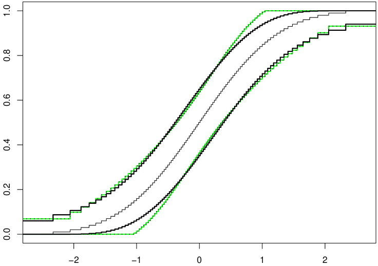
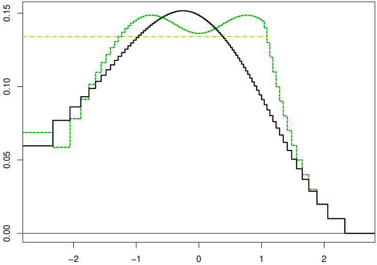
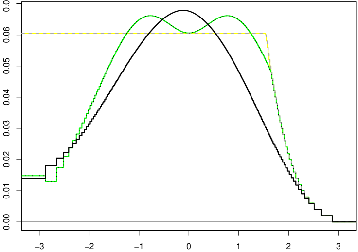
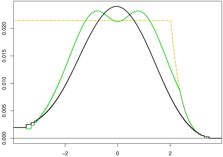
In Example 3.11, we illustrated the impact of on the confidence bands by comparing these bands for , and . Figure 7 provides these comparisons for the same and but . Figure 8 shows analogous pictures for .
