Higher moments of primordial non-Gaussianity and N-body simulations

Saroj Adhikari    Sarah Shandera    Neal Dalal
Abstract

We perform cosmological N-body simulations with non-Gaussian initial conditions generated from two independent fields. The dominant contribution to the perturbations comes from a purely Gaussian field, but we allow the second field to have local non-Gaussianity that need not be weak. This scenario allows us to adjust the relative importance of non-Gaussian contributions beyond the skewness, producing a scaling of the higher moments different from (and stronger than) the scaling in the usual single field local ansatz. We compare semi-analytic prescriptions for the non-Gaussian mass function, large scale halo bias, and stochastic bias against the simulation results. We discuss applications of this work to large scale structure measurements that can test a wider range of models for the primordial fluctuations than is usually explored.

1 Introduction

Recently, the Planck satellite mission reported tight constraints on primordial non-Gaussianity from measurements of the Cosmic Microwave Background (CMB) [1]. They find the amplitude of the local, equilateral and orthogonal type bispectrum to be fNLlocal=2.7±5.8superscriptsubscript𝑓NLlocalplus-or-minus2.75.8f_{\rm NL}^{\rm local}=2.7\pm 5.8, fNLequil=42±75superscriptsubscript𝑓NLequilplus-or-minus4275f_{\rm NL}^{\rm equil}=-42\pm 75, and fNLortho=25±39superscriptsubscript𝑓NLorthoplus-or-minus2539f_{\rm NL}^{\rm ortho}=-25\pm 39 respectively at 1σ1𝜎1\sigma level. While these results show that the primordial fluctuations were remarkably Gaussian, they still leave room for interesting signatures of primordial physics to be found in statistics beyond the power spectrum: minimal, single field models predict non-Gaussianity that is about two orders of magnitude below these constraints. Non-Gaussianity is such an informative tool for inflationary physics that it is crucial to push observational bounds as far as possible. A number of forecasts have shown that the use of clustering data from future large scale structure surveys can constrain fNLlocalsuperscriptsubscript𝑓NLlocalf_{\rm NL}^{\rm local} with σ(fNL)(110)𝜎subscript𝑓NL110\sigma(f_{\rm NL})\approx(1-10) [2, 3, 4, 5, 6, 7]. In addition, the galaxy bispectrum is a promising way to probe many shapes to the fNL𝒪(110)similar-tosubscript𝑓NL𝒪110f_{\rm NL}\sim\mathcal{O}(1-10) level [8, 9, 10]. The constraints from large scale structure (LSS) —whether consistent with the CMB measurements or in tension — will provide interesting and useful complementary results.

In the inflationary scenario, non-Gaussian signatures in the primordial density fluctuations depend on the details of interactions of the inflaton or other fields relevant for generating the perturbations; therefore, any detection (or the lack) of primordial non-Gaussianity tells us about the dynamics of those fields. Furthermore, if non-Gaussianity is detected, we expect to see patterns in the correlations that are consistent with perturbation theory (in contrast to apparently independent statistics at each order, for example). The simplest such pattern is in the relative amplitudes of higher order statistics, or, how the amplitudes of the correlation functions of the gravitational potential, Φn(x)delimited-⟨⟩superscriptΦ𝑛𝑥\langle\Phi^{n}(\vec{x})\rangle, scale with order n𝑛n. The relative scaling of higher moments falls into a fairly narrow range of behaviors in inflationary models [11].

Thanks to the non-linearity of structure formation, the statistics of objects in the late universe contain information about the entire series of higher order moments of the initial density fluctuations. This is especially straightforward to see in number counts of galaxy clusters [12]. While information about higher moments is clearly non-trivial to extract when non-Gaussianity is weak, some constraints with current data are already affected by assumptions about higher order moments. For example, [13] reports constraints on primordial non-Gaussianity using a sample of 237 X-ray clusters from the ROSAT All-Sky Survey [14]. Their analysis clearly suggests that it is important to take the scaling of moments into account when deriving constraints on fNLsubscript𝑓NLf_{\rm NL} from cluster number counts. The results presented in this paper will be useful for further studies in the same direction. Tighter constraints could likely be achieved with current data by combining the X-ray clusters with SZ detected clusters that have been separately used to constrain non-Gaussianity [15, 16, 17]. In addition, the eROSITA survey [6] and third generation surveys detecting clusters via the Sunyaev-Zel’dovich effect are expected to provide much larger samples of clusters in the next few years. It will be interesting to revisit the non-Gaussian analysis when that data becomes available. Other large scale structure statistics, including the power spectrum and bispectrum of galaxies, also contain contributions from higher order primordial statistics. Constraints on non-Gaussianity from those observables are still being developed, and will ultimately be very powerful (constraints obtained to date include [18, 19, 20, 21, 22, 23, 24, 25, 26]). To make full use of them it is important to understand the signatures of the full spectrum of non-Gaussian models predicted from inflation.

In this paper, we will use a slight variant of the popular local ansatz of primordial non-Gaussianity in order to generate two different scalings of the n𝑛n-point functions and study how the scalings can be distinguished. For the usual local ansatz with hierarchical scaling, many groups have already performed simulations [27, 28, 29, 30, 31, 32] and found that the semi-analytic prescription of [12] for the non-Gaussian mass function works well. Here we will also test the validity of the mass function proposed in [11] and used in [13] for another scaling that is well motivated by inflationary models. In addition to looking at the mass function, we will also look at a signature of the shape (momentum dependence) of local type non-Gaussianity using the scale dependent halo bias [33], and at the stochastic bias on large scales [34]. Subleading contributions to the bias and leading contributions to the stochastic bias are sensitive to non-Gaussianity beyond the skewness.

The rest of the paper is structured as follows: in Section 2 we introduce our two field model and the scaling of the higher moments. In Section 3 we present the analytical calculations for the mass function of halos, bias, and stochasticity (with details relegated to the appendices). In Section 4 we describe our simulations, and then compare the output from simulations to the analytical calculations in Section 5. Finally, we conclude in Section 6.

2 Model

In the usual local ansatz, the Bardeen potential Φ(x)Φ𝑥\Phi(x) has non-Gaussian statistics thanks to a contribution from a non-linear, local function of a Gaussian field ψG(x)subscript𝜓𝐺𝑥\psi_{G}(\vec{x}):

Φ(x)=ψG(x)+fNL(ψG(x)2ψG(x)2).Φ𝑥subscript𝜓𝐺𝑥subscript𝑓NLsubscript𝜓𝐺superscript𝑥2delimited-⟨⟩subscript𝜓𝐺superscript𝑥2\displaystyle\Phi(\vec{x})=\psi_{G}(\vec{x})+f_{\rm NL}\left(\psi_{G}(\vec{x})^{2}-\langle\psi_{G}(\vec{x})^{2}\rangle\right)\;. (2.1)

Here fNLsubscript𝑓NLf_{\rm NL} parametrizes the size of the non-linear term and the level of non-Gaussianity. Non-Gaussianity of this type is usually thought of as produced by a light field that is not the inflaton [35, 36, 37, 38, 39, 40], and in fact cannot be generated by single field inflation proceeding along the attractor solution with modes in the Bunch-Davies vacuum [41, 42].

The two-point statistics (the power spectrum) of the fluctuations are well measured from CMB observations for about three decades in scale [43, 44, 45]. The amplitude of the three point function gives the skewness of the distribution of ΦΦ\Phi, and is also well-constrained by the CMB [1]. Higher order correlation functions are more difficult to measure in the data. We would like to see if we can get some handle on the structure of the scaling of these higher order statistics of ΦΦ\Phi. For this purpose, we define the dimensionless moments nsubscript𝑛\mathcal{M}_{n}:

n=Φ(x)ncΦ(x)2cn/2subscript𝑛subscriptdelimited-⟨⟩Φsuperscript𝑥𝑛𝑐superscriptsubscriptdelimited-⟨⟩Φsuperscript𝑥2𝑐𝑛2\displaystyle\mathcal{M}_{n}=\frac{\langle\Phi(\vec{x})^{n}\rangle_{c}}{\langle\Phi(\vec{x})^{2}\rangle_{c}^{n/2}} (2.2)

where the subscript c𝑐c indicates that we take the connected part of the n𝑛n-point function.

Two scalings:

For the local model given by Eq. (2.1), the moments scale approximately as

nhierAn(36)n2,n>2formulae-sequencesubscriptsuperscripthier𝑛subscript𝐴𝑛superscriptsubscript36𝑛2𝑛2\mathcal{M}^{\rm hier}_{n}\approx A_{n}\left(\frac{\mathcal{M}_{3}}{6}\right)^{n-2}\;,\;\;\;n>2 (2.3)

where An=2n3n!subscript𝐴𝑛superscript2𝑛3𝑛A_{n}=2^{n-3}n! comes out of combinatorics. The numerical coefficients in this scaling are not quite precise because of the difference in integrals over momenta at each order n𝑛n (see Appendix A), but the parametric dependence on the amplitude of the skewness and the total power is fixed. This is the behavior of the moments (which we label ‘hierarchical’ scaling) for fNLsubscript𝑓NLf_{\rm NL} not too large i.e. when 2fNL2σ21much-less-than2superscriptsubscript𝑓NL2superscript𝜎212f_{\rm NL}^{2}\sigma^{2}\ll 1, where σ2=ψG(x)2superscript𝜎2delimited-⟨⟩subscript𝜓𝐺superscript𝑥2\sigma^{2}=\langle\psi_{G}(\vec{x})^{2}\rangle. However, if 2fNL2σ21much-greater-than2superscriptsubscript𝑓NL2superscript𝜎212f_{\rm NL}^{2}\sigma^{2}\gg 1, the moments scale differently:

nfeederBn(38)n/3,n>2formulae-sequencesubscriptsuperscriptfeeder𝑛subscript𝐵𝑛superscriptsubscript38𝑛3𝑛2\mathcal{M}^{\rm feeder}_{n}\approx B_{n}\left(\frac{\mathcal{M}_{3}}{8}\right)^{n/3}\;,\;\;\;n>2 (2.4)

where Bn=2n1(n1)!subscript𝐵𝑛superscript2𝑛1𝑛1B_{n}=2^{n-1}(n-1)!. In the single source case, this is far too non-Gaussian to be consistent with observations. Therefore, we consider the following two source model [46, 34, 11]:

Φ(x)=ϕG(x)+ψG(x)+f~NL(ψG(x)2ψG(x)2)Φ𝑥subscriptitalic-ϕ𝐺𝑥subscript𝜓𝐺𝑥subscript~𝑓NLsubscript𝜓𝐺superscript𝑥2delimited-⟨⟩subscript𝜓𝐺superscript𝑥2\displaystyle\Phi(\vec{x})=\phi_{G}(\vec{x})+\psi_{G}(\vec{x})+\tilde{f}_{\rm NL}\left(\psi_{G}(\vec{x})^{2}-\langle\psi_{G}(\vec{x})^{2}\rangle\right) (2.5)

where the two Gaussian fields ψG(x)subscript𝜓𝐺𝑥\psi_{G}(\vec{x}) and ϕG(x)subscriptitalic-ϕ𝐺𝑥\phi_{G}(\vec{x}) are uncorrelated i.e. ϕG(x)ψG(x)=0delimited-⟨⟩subscriptitalic-ϕ𝐺𝑥subscript𝜓𝐺𝑥0\langle\phi_{G}(\vec{x})\psi_{G}(\vec{x})\rangle=0.

To express the correlations in the gravitational potential ΦΦ\Phi in terms of the amplitude of fluctuations in just one of the source fields we define

q=Pψ,G(k)Pψ,G(k)+Pϕ(k),𝑞subscript𝑃𝜓𝐺𝑘subscript𝑃𝜓𝐺𝑘subscript𝑃italic-ϕ𝑘q=\frac{P_{\psi,G}(k)}{P_{\psi,G}(k)+P_{\phi}(k)}\;, (2.6)

the ratio of the contribution of the Gaussian part of the field ψ𝜓\psi to the total Gaussian power. Pψ,G(k)subscript𝑃𝜓𝐺𝑘P_{\psi,G}(k) is defined by

ψG(k)ψG(k)=(2π)3δD3(k+k)Pψ,G(k).delimited-⟨⟩subscript𝜓𝐺𝑘subscript𝜓𝐺superscript𝑘superscript2𝜋3subscriptsuperscript𝛿3𝐷𝑘superscript𝑘subscript𝑃𝜓𝐺𝑘\langle\psi_{G}(\vec{k})\psi_{G}(\vec{k}^{\prime})\rangle=(2\pi)^{3}\delta^{3}_{D}(\vec{k}+\vec{k}^{\prime})P_{\psi,G}(k)\;. (2.7)

For simplicity we assume both Gaussian components have constant, identical spectral indices but different amplitudes: Pϕ(k)=2π2𝒫ϕ(k)/k3subscript𝑃italic-ϕ𝑘2superscript𝜋2subscript𝒫italic-ϕ𝑘superscript𝑘3P_{\phi}(k)=2\pi^{2}\mathcal{P}_{\phi}(k)/k^{3} with 𝒫ϕ(k)=Aϕ(kk0)γsubscript𝒫italic-ϕ𝑘subscript𝐴italic-ϕsuperscript𝑘subscript𝑘0𝛾\mathcal{P}_{\phi}(k)=A_{\phi}\left(\frac{k}{k_{0}}\right)^{\gamma}, and similarly for Pψ,Gsubscript𝑃𝜓𝐺P_{\psi,G} (with the same index γ𝛾\gamma but a different amplitude Aψsubscript𝐴𝜓A_{\psi}). With this choice, q𝑞q is a scale-independent constant.

The power spectrum, bispectrum, and trispectrum in our model are:

PΦ(k)subscript𝑃Φ𝑘\displaystyle P_{\Phi}(k) =\displaystyle= [1q+f~NL2I1(k)𝒫ψ,G(k)]Pψ,G(k)delimited-[]1𝑞superscriptsubscript~𝑓NL2subscript𝐼1𝑘subscript𝒫𝜓𝐺𝑘subscript𝑃𝜓𝐺𝑘\displaystyle\left[\frac{1}{q}+\tilde{f}_{\rm NL}^{2}I_{1}(k)\mathcal{P}_{\psi,G}(k)\right]P_{\psi,G}(k)
=\displaystyle= [11q+(qf~NL1q)2I1(k)𝒫ϕ(k)]Pϕ(k)delimited-[]11𝑞superscript𝑞subscript~𝑓NL1𝑞2subscript𝐼1𝑘subscript𝒫italic-ϕ𝑘subscript𝑃italic-ϕ𝑘\displaystyle\left[\frac{1}{1-q}+\left(\frac{q\tilde{f}_{\rm NL}}{1-q}\right)^{2}I_{1}(k)\mathcal{P}_{\phi}(k)\right]P_{\phi}(k)
B(k1,k2,k3)𝐵subscript𝑘1subscript𝑘2subscript𝑘3\displaystyle B(k_{1},k_{2},k_{3}) =\displaystyle= 2f~NL[Pψ,G(k1)Pψ,G(k2)+2perm]2subscript~𝑓NLdelimited-[]subscript𝑃𝜓𝐺subscript𝑘1subscript𝑃𝜓𝐺subscript𝑘22perm\displaystyle 2\tilde{f}_{\rm NL}\left[P_{\psi,G}(k_{1})P_{\psi,G}(k_{2})+2\;{\rm perm}\right] (2.9)
+2f~NL3[d3p(2π)3Pψ,G(p)Pψ,G(|k1p|)Pψ,G(|k2+p|)+3perm]2superscriptsubscript~𝑓NL3delimited-[]superscript𝑑3𝑝superscript2𝜋3subscript𝑃𝜓𝐺𝑝subscript𝑃𝜓𝐺subscript𝑘1𝑝subscript𝑃𝜓𝐺subscript𝑘2𝑝3perm\displaystyle+2\tilde{f}_{\rm NL}^{3}\left[\int\frac{d^{3}\vec{p}}{(2\pi)^{3}}P_{\psi,G}(p)P_{\psi,G}(|\vec{k_{1}}-\vec{p}|)P_{\psi,G}(|\vec{k_{2}}+\vec{p}|)+3\;{\rm perm}\right]
T(k1,k2,k3,k4)𝑇subscript𝑘1subscript𝑘2subscript𝑘3subscript𝑘4\displaystyle T(k_{1},k_{2},k_{3},k_{4}) =\displaystyle= 2f~NL2[Pψ,G(k1)Pψ(k2)Pψ,G(|k1+k3|)+23perm]2superscriptsubscript~𝑓NL2delimited-[]subscript𝑃𝜓𝐺subscript𝑘1subscript𝑃𝜓subscript𝑘2subscript𝑃𝜓𝐺subscript𝑘1subscript𝑘323perm\displaystyle 2\tilde{f}_{\rm NL}^{2}\left[P_{\psi,G}(k_{1})P_{\psi}(k_{2})P_{\psi,G}(|\vec{k_{1}}+\vec{k_{3}}|)+23\;{\rm perm}\right] (2.10)
+f~NL4[d3p(2π)3Pψ,G(p)Pψ,G(|k1p|)Pψ,G(|k2+p|)Pψ,G(|k2+k4+p|)\displaystyle+\tilde{f}_{\rm NL}^{4}\left[\int\frac{d^{3}\vec{p}}{(2\pi)^{3}}P_{\psi,G}(p)P_{\psi,G}(|\vec{k_{1}}-\vec{p}|)P_{\psi,G}(|\vec{k_{2}}+\vec{p}|)P_{\psi,G}(|\vec{k_{2}}+\vec{k_{4}}+\vec{p}|)\right.
+47perm]\displaystyle\left.+47\;{\rm perm}\right]

where we have defined I1(k)subscript𝐼1𝑘I_{1}(k) as

I1(k)subscript𝐼1𝑘\displaystyle I_{1}(k) =\displaystyle= kminkkmaxk𝑑u11𝑑μ[uγ1(1+u2+2μu)γ32]superscriptsubscriptsubscript𝑘𝑚𝑖𝑛𝑘subscript𝑘𝑚𝑎𝑥𝑘differential-d𝑢superscriptsubscript11differential-d𝜇delimited-[]superscript𝑢𝛾1superscript1superscript𝑢22𝜇𝑢𝛾32\displaystyle\int_{\frac{k_{min}}{k}}^{\frac{k_{max}}{k}}du\int_{-1}^{1}d\mu\left[u^{\gamma-1}(1+u^{2}+2\mu u)^{\frac{\gamma-3}{2}}\right] (2.11)

Here, kmin=2π/Lsubscript𝑘𝑚𝑖𝑛2𝜋𝐿k_{min}=2\pi/L is the infrared cutoff for a boxsize of L𝐿L. In general, we do not know of the size of the universe beyond our observable universe, but for our purposes, the simulation box size L𝐿L is the natural choice. kmaxsubscript𝑘𝑚𝑎𝑥k_{max} is the scale leaving the horizon at the initial epoch [47]. The above integrals converge for large values of kmaxsubscript𝑘𝑚𝑎𝑥k_{max}. For the computations to compare with simulations we set kmax=Np1/3kminsubscript𝑘𝑚𝑎𝑥superscriptsubscript𝑁𝑝13subscript𝑘𝑚𝑖𝑛k_{max}=N_{p}^{1/3}k_{min}, where Npsubscript𝑁𝑝N_{p} is the number of particles in a simulation. To arrive at the expressions quoted above, we have used

d3p(2π)3Pψ(p)Pψ(|kp|)superscript𝑑3𝑝superscript2𝜋3subscript𝑃𝜓𝑝subscript𝑃𝜓𝑘𝑝\displaystyle\int\frac{d^{3}\vec{p}}{(2\pi)^{3}}P_{\psi}(p)P_{\psi}(|\vec{k}-\vec{p}|) =\displaystyle= 12I1(k)𝒫ψ(k)Pψ(k).12subscript𝐼1𝑘subscript𝒫𝜓𝑘subscript𝑃𝜓𝑘\displaystyle\frac{1}{2}I_{1}(k)\mathcal{P}_{\psi}(k)P_{\psi}(k)\;. (2.12)

In Equations (LABEL:eq:powerspectrum), (2.9) and (2.10) we have included terms that are usually sub-dominant in the case of single field, weakly non-Gaussian local ansatz. In our model, these terms are important when the field ψ𝜓\psi is strongly non-Gaussian. To discuss the observational constraints on (q,f~NL)𝑞subscript~𝑓NL(q,\tilde{f}_{\rm NL}), let’s consider 𝒫Φ(k)109subscript𝒫Φ𝑘superscript109\mathcal{P}_{\Phi}(k)\approx 10^{-9}, I1(k)10subscript𝐼1𝑘10I_{1}(k)\approx 10 and fNL𝒪(10)less-than-or-similar-tosubscript𝑓NL𝒪10f_{\rm NL}\lesssim\mathcal{O}(10). Observational constraint from small non-Gaussianity can be satisfied by making (q2f~NL)𝒪(10)less-than-or-similar-tosuperscript𝑞2subscript~𝑓NL𝒪10(q^{2}\tilde{f}_{\rm NL})\lesssim\mathcal{O}(10) and (qf~NL)3𝒪(109)less-than-or-similar-tosuperscript𝑞subscript~𝑓NL3𝒪superscript109(q\tilde{f}_{\rm NL})^{3}\lesssim\mathcal{O}(10^{9}), in which case the Gaussian contributions (Pϕ(k)+Pψ,G(k)subscript𝑃italic-ϕ𝑘subscript𝑃𝜓𝐺𝑘P_{\phi}(k)+P_{\psi,G}(k)) dominate the total power spectrum in Eq.(LABEL:eq:powerspectrum) as well. Notice that the non-Gaussian contribution to the power can shift the spectral index slightly, so that when the ψ𝜓\psi field is strongly non-Gaussian the measured spectral index is close to, but not identical to, the spectral index of the Gaussian components111The new, integral terms have slightly different shapes than the usual terms. The difference, however, is small—approximately described by lnkL𝑘𝐿\ln{kL} which has a weak dependence on k𝑘k. These terms are also infrared divergent. For the purpose of comparing with the results from N-body simulations, the box size L𝐿L of the simulation provides a natural cutoff [30]. We will only look at quantities well enough inside the volume that the arbitrary size L𝐿L doesn’t affect our results., ns1γsubscript𝑛𝑠1𝛾n_{s}-1\neq\gamma.

If q1much-less-than𝑞1q\ll 1 and (qf~NL)3109much-less-thansuperscript𝑞subscript~𝑓NL3superscript109(q\tilde{f}_{\rm NL})^{3}\ll 10^{9}, then one can generate the feeder scaling in Eq.(2.4) without being inconsistent with the current observations of power spectrum and bounds on non-Gaussianity. The feeder scaling dominates when the condition qf~NL2109much-greater-than𝑞superscriptsubscript~𝑓NL2superscript109q\tilde{f}_{\rm NL}^{2}\gg 10^{9} is satisfied. This scaling, or a hybrid between hierarchical and feeder scaling, arises in particle physics scenarios where a second, non-Gaussian field couples to the inflaton and provides an extra source for the fluctuations [11, 48]. However, those scenarios differ from the model here because they most often generate bispectra not of the local type222One can also argue on statistical grounds that our observable universe is unlikely to have local non-Gaussianity of the type written in Eq.(2.5) with large f~NLsubscript~𝑓NL\tilde{f}_{\rm NL} if inflation lasts much longer than 55 e-folds [49, 50]).. Here we are using the two field, local model primarily as a phenomenological tool, easy to implement in N-body simulations, to generate the feeder-type scaling of moments rather than as the output of a particular inflation model. The mass function is sensitive only to the integrated moments, not the shape, so this is a useful test of how different scalings affect the number of objects in a non-Gaussian cosmology.

3 Abundance and Clustering Statistics

In this section we present the analytic predictions for the effect of locally non-Gaussian, two source initial conditions on the abundance and clustering of dark matter halos.

At large scales, the evolution of the density contrast is well described by linear perturbation theory, and the density contrast in Fourier space at redshift z𝑧z is given by δ(k,z)=α(k,z)Φ(k)𝛿𝑘𝑧𝛼𝑘𝑧Φ𝑘\delta(\vec{k},z)=\alpha(k,z)\Phi(\vec{k}), where

α(k,z)=23k2T(k)D(z)H02Ωm.𝛼𝑘𝑧23superscript𝑘2𝑇𝑘𝐷𝑧superscriptsubscript𝐻02subscriptΩ𝑚\displaystyle\alpha(k,z)=\frac{2}{3}\frac{k^{2}T(k)D(z)}{H_{0}^{2}\Omega_{m}}\;. (3.1)

Here T(k)𝑇𝑘T(k) is the transfer function, D(z)𝐷𝑧D(z) is the growth function, H0subscript𝐻0H_{0} is the Hubble scale today, and ΩmsubscriptΩ𝑚\Omega_{m} is the energy density in matter today (compared to critical density). The smoothed density contrast, similarly, is δR(k,z)=WR(k)α(k,z)Φ(k)subscript𝛿𝑅𝑘𝑧subscript𝑊𝑅𝑘𝛼𝑘𝑧Φ𝑘\delta_{R}(\vec{k},z)=W_{R}(k)\alpha(k,z)\Phi(\vec{k}), where

WR(k)=3sin(kR)3(kR)cos(kR)(kR)3subscript𝑊𝑅𝑘3𝑘𝑅3𝑘𝑅𝑘𝑅superscript𝑘𝑅3\displaystyle W_{R}(k)=\frac{3\sin({kR})-3(kR)\cos({kR})}{(kR)^{3}} (3.2)

is the smoothing function (here the Fourier transform of the real space top-hat). Note that we will generally suppress the z𝑧z dependence in α(k,z)𝛼𝑘𝑧\alpha(k,z) and δ(k,z)𝛿𝑘𝑧\delta(\vec{k},z) in this paper, and usually write α(k)𝛼𝑘\alpha(k) and δ(k)𝛿𝑘\delta(\vec{k}) only. We can now compute the connected n-point functions of the smoothed density contrast in real space:

δR(x)nc(z)=d3k1(2π)3d3kn(2π)3δR(k1,z)δR(kn,z)csubscriptdelimited-⟨⟩subscript𝛿𝑅superscript𝑥𝑛𝑐𝑧superscript𝑑3subscript𝑘1superscript2𝜋3superscript𝑑3subscript𝑘𝑛superscript2𝜋3subscriptdelimited-⟨⟩subscript𝛿𝑅subscript𝑘1𝑧subscript𝛿𝑅subscript𝑘𝑛𝑧𝑐\displaystyle\langle\delta_{R}(\vec{x})^{n}\rangle_{c}(z)=\int\frac{d^{3}\vec{k_{1}}}{(2\pi)^{3}}\dots\int\frac{d^{3}\vec{k_{n}}}{(2\pi)^{3}}\langle\delta_{R}(\vec{k_{1}},z)\dots\delta_{R}(\vec{k_{n}},z)\rangle_{c} (3.3)

and therefore the dimensionless moments of smoothed density fields: n,R=δR(x)ncδR(x)2n/2subscript𝑛𝑅subscriptdelimited-⟨⟩subscript𝛿𝑅superscript𝑥𝑛𝑐superscriptdelimited-⟨⟩subscript𝛿𝑅superscript𝑥2𝑛2\mathcal{M}_{n,R}=\frac{\langle\delta_{R}(\vec{x})^{n}\rangle_{c}}{\langle\delta_{R}(\vec{x})^{2}\rangle^{n/2}}. Note that the dimensionless moments are redshift independent. Eq.(3.3) can be separated into two components: (i) of 𝒪(f~NLn2)𝒪superscriptsubscript~𝑓NL𝑛2\mathcal{O}(\tilde{f}_{\rm NL}^{n-2}) and (ii) of 𝒪(f~NLn)𝒪superscriptsubscript~𝑓NL𝑛\mathcal{O}(\tilde{f}_{\rm NL}^{n}), corresponding to contributions to the hierarchical and feeder scalings respectively. Some of these integrals, with a brief summary of our method to evaluate them, are given in Appendix A.

3.1 Mass function

We follow previous studies of non-Gaussian mass functions in that we calculate the ratio R=nNG(M,z)nG(M,z)𝑅subscript𝑛𝑁𝐺𝑀𝑧subscript𝑛𝐺𝑀𝑧R=\frac{n_{NG}(M,z)}{n_{G}(M,z)} of the number density in the presence of non-Gaussianity, nNGsubscript𝑛𝑁𝐺n_{NG}, to the number density for Gaussian initial conditions, nGsubscript𝑛𝐺n_{G}, for a particular halo mass M𝑀M at some redshift z𝑧z using the Press-Schechter formalism [51]. The fractional volume F(M)𝐹𝑀F(M) of dark matter in the collapsed structures (halos) is proportional to δcP(δM)𝑑δMsuperscriptsubscriptsubscript𝛿𝑐𝑃subscript𝛿𝑀differential-dsubscript𝛿𝑀\int_{\delta_{c}}^{\infty}P(\delta_{M})d\delta_{M}, where δcsubscript𝛿𝑐\delta_{c} is the critical value of the smoothed density contrast δMsubscript𝛿𝑀\delta_{M} above which the dark matter in a region collapses to form halos and P(δM)𝑃subscript𝛿𝑀P(\delta_{M}) is a probability density function (PDF). Here we have written the smoothing scale in terms of the mass M𝑀M rather than the smoothing radius R𝑅R; they are simply related by M=43πR3ρm𝑀43𝜋superscript𝑅3subscript𝜌𝑚M=\frac{4}{3}\pi R^{3}\rho_{m}, where ρmsubscript𝜌𝑚\rho_{m} is the mean matter density of the universe. Then, the number density (mass function) is given by:

dndM=dF(M)dM×ρmM𝑑𝑛𝑑𝑀𝑑𝐹𝑀𝑑𝑀subscript𝜌𝑚𝑀\displaystyle\frac{dn}{dM}=\frac{dF(M)}{dM}\times\frac{\rho_{m}}{M} (3.4)

For a Gaussian PDF, one can easily perform the integration to find a prediction for the mass function. However, the result is known to be only an approximation and in practice Gaussian mass functions are calibrated on simulations [52].

To apply the method above in case of non-Gaussian initial conditions we need a non-Gaussian PDF. The Petrov expansion [53] (which generalizes the Edgeworth expansion [54, 55]) expresses a non-Gaussian PDF as a series in the cumulants of the distribution. In terms of n,Rsubscript𝑛𝑅\mathcal{M}_{n,R}’s, this is:

P(ν,R)𝑃𝜈𝑅\displaystyle P(\nu,R) =\displaystyle= eν2/22π[1+s=1kmHs+2r(ν)m=1s1km!(m+2,R(m+2)!)km]superscript𝑒superscript𝜈222𝜋delimited-[]1superscriptsubscript𝑠1subscriptsubscript𝑘𝑚subscript𝐻𝑠2𝑟𝜈superscriptsubscriptproduct𝑚1𝑠1subscript𝑘𝑚superscriptsubscript𝑚2𝑅𝑚2subscript𝑘𝑚\displaystyle\frac{e^{-\nu^{2}/2}}{\sqrt{2\pi}}\left[1+\sum_{s=1}^{\infty}\sum_{k_{m}}H_{s+2r}(\nu)\prod_{m=1}^{s}\frac{1}{k_{m}!}\left(\frac{\mathcal{M}_{m+2,R}}{(m+2)!}\right)^{k_{m}}\right] (3.5)

where ν=δMσM𝜈subscript𝛿𝑀subscript𝜎𝑀\nu=\frac{\delta_{M}}{\sigma_{M}}, σM=δM2subscript𝜎𝑀delimited-⟨⟩superscriptsubscript𝛿𝑀2\sigma_{M}=\sqrt{\langle\delta_{M}^{2}\rangle} and Hnsubscript𝐻𝑛H_{n}’s are the Hermite polynomials defined as Hn(ν)=(1)neν2/2dndνneν2/2subscript𝐻𝑛𝜈superscript1𝑛superscript𝑒superscript𝜈22superscript𝑑𝑛𝑑superscript𝜈𝑛superscript𝑒superscript𝜈22H_{n}(\nu)=(-1)^{n}e^{\nu^{2}/2}\frac{d^{n}}{d\nu^{n}}e^{-\nu^{2}/2}. The second sum is over the non-negative integer members of the set {km}subscript𝑘𝑚\{k_{m}\} that satisfy

k1+2k2++sks=s.subscript𝑘12subscript𝑘2𝑠subscript𝑘𝑠𝑠k_{1}+2k_{2}+\dots+sk_{s}=s\;. (3.6)

For each set rk1+k2++ks𝑟subscript𝑘1subscript𝑘2subscript𝑘𝑠r\equiv k_{1}+k_{2}+\dots+k_{s}. This series can be integrated term by term to obtain F(M)𝐹𝑀F(M), and with Eq.(3.4) gives ratio of non-Gaussian mass function to Gaussian mass function [13]

nNGnG1+F1h,f(M)F0(M)+F2h,f(M)F0(M)+subscript𝑛𝑁𝐺subscript𝑛𝐺1superscriptsubscript𝐹1superscript𝑓𝑀superscriptsubscript𝐹0𝑀superscriptsubscript𝐹2superscript𝑓𝑀superscriptsubscript𝐹0𝑀\displaystyle\frac{n_{NG}}{n_{G}}\approx 1+\frac{F_{1}^{h,f^{\prime}}(M)}{F_{0}^{\prime}(M)}+\frac{F_{2}^{h,f^{\prime}}(M)}{F_{0}^{\prime}(M)}+\dots (3.7)

where

F0(M)=νc(M)2πe12νc(M)2,νc=δcσM.formulae-sequencesuperscriptsubscript𝐹0𝑀superscriptsubscript𝜈𝑐𝑀2𝜋superscript𝑒12subscript𝜈𝑐superscript𝑀2subscript𝜈𝑐subscript𝛿𝑐subscript𝜎𝑀\displaystyle F_{0}^{\prime}(M)=-\frac{\nu_{c}^{\prime}(M)}{\sqrt{2\pi}}e^{-\frac{1}{2}\nu_{c}(M)^{2}}\;,\;\;\;\nu_{c}=\frac{\delta_{c}}{\sigma_{M}}. (3.8)

The two superscripts h,f𝑓h,f indicate that the set of terms that are of the same order depends on whether higher order cumulants have hierarchical (hh) or feeder (f𝑓f) scaling. Formally grouping terms assuming the scalings in Eq(2.3) or Eq.(2.4) are exact gives (for s1𝑠1s\geq 1)

Fsh(ν)superscriptsubscript𝐹𝑠superscript𝜈\displaystyle F_{s}^{h^{\prime}}(\nu) =\displaystyle= F0{km}h{Hs+2rm=1s1km!(m+2,R(m+2)!)km+Hs+2r1σνddσ[m=1s1km!(m+2,R(m+2)!)km]}superscriptsubscript𝐹0subscriptsubscriptsubscript𝑘𝑚subscript𝐻𝑠2𝑟superscriptsubscriptproduct𝑚1𝑠1subscript𝑘𝑚superscriptsubscript𝑚2𝑅𝑚2subscript𝑘𝑚subscript𝐻𝑠2𝑟1𝜎𝜈𝑑𝑑𝜎delimited-[]superscriptsubscriptproduct𝑚1𝑠1subscript𝑘𝑚superscriptsubscript𝑚2𝑅𝑚2subscript𝑘𝑚\displaystyle F_{0}^{\prime}\sum_{\{k_{m}\}_{h}}\!\!\left\{\!H_{\small{s+2r}}\!\prod_{m=1}^{s}\frac{1}{k_{m}!}\left(\frac{\mathcal{M}_{m+2,R}}{(m+2)!}\right)^{k_{m}}\!\!\!+H_{s+2r-1}\frac{\sigma}{\nu}\frac{d}{d\sigma}\left[\prod_{m=1}^{s}\frac{1}{k_{m}!}\left(\frac{\mathcal{M}_{m+2,R}}{(m+2)!}\right)^{k_{m}}\right]\right\}
Fsf(ν)superscriptsubscript𝐹𝑠superscript𝑓𝜈\displaystyle F_{s}^{f^{\prime}}(\nu) =\displaystyle= F0{km}f{Hs+2m=1s1km!(m+2,R(m+2)!)km+Hs+1σνddσ[m=1s1km!(m+2,R(m+2)!)km]}.superscriptsubscript𝐹0subscriptsubscriptsubscript𝑘𝑚𝑓subscript𝐻𝑠2superscriptsubscriptproduct𝑚1𝑠1subscript𝑘𝑚superscriptsubscript𝑚2𝑅𝑚2subscript𝑘𝑚subscript𝐻𝑠1𝜎𝜈𝑑𝑑𝜎delimited-[]superscriptsubscriptproduct𝑚1𝑠1subscript𝑘𝑚superscriptsubscript𝑚2𝑅𝑚2subscript𝑘𝑚\displaystyle F_{0}^{\prime}\sum_{\{k_{m}\}_{f}}\!\!\left\{H_{s+2}\prod_{m=1}^{s}\frac{1}{k_{m}!}\left(\frac{\mathcal{M}_{m+2,R}}{(m+2)!}\right)^{k_{m}}\!\!\!+H_{s+1}\frac{\sigma}{\nu}\frac{d}{d\sigma}\left[\prod_{m=1}^{s}\frac{1}{k_{m}!}\left(\frac{\mathcal{M}_{m+2,R}}{(m+2)!}\right)^{k_{m}}\right]\right\}\;.

The prime stands for the derivative with respect to the halo mass M𝑀M. In the hierarchical case, the sets {km}hsubscriptsubscript𝑘𝑚\{k_{m}\}_{h} still satisfy Eq.(3.6), while for feeder scaling the {km}fsubscriptsubscript𝑘𝑚𝑓\{k_{m}\}_{f} are the sets of non-negative integer solutions to 3k1+4k2++(s+2)ks=s+23subscript𝑘14subscript𝑘2𝑠2subscript𝑘𝑠𝑠23k_{1}+4k_{2}+\dots+(s+2)k_{s}=s+2.

Eq.(3.7) assumes that the two point statistics of the smoothed linear density contrast (i.e δM2delimited-⟨⟩subscriptsuperscript𝛿2𝑀\langle\delta^{2}_{M}\rangle) are the same for the non-Gaussian and the Gaussian cases (not that the Gaussian contributions to δM2delimited-⟨⟩subscriptsuperscript𝛿2𝑀\langle\delta^{2}_{M}\rangle are the same). However, this is difficult to maintain at all scales in our simulations. We require the two point clustering statistics to match at a particular scale R=8Mpc/h𝑅8MpchR=8\;\rm Mpc/h, but do not correct for the shift to the spectral index coming from the non-Gaussian term in the power spectrum. As a result, on scales other than R=8Mpc/h𝑅8MpchR=8\;\rm Mpc/h we need to make a distinction between F0,NG(M)superscriptsubscript𝐹0𝑁𝐺𝑀F_{0,NG}^{\prime}(M) for the non-Gaussian cosmology and F0,G(M)superscriptsubscript𝐹0𝐺𝑀F_{0,G}^{\prime}(M) for the Gaussian cosmology. In that case, there is an extra (mass or scale dependent) factor f1(M)subscript𝑓1𝑀f_{1}(M) in the ratio nNGnGsubscript𝑛𝑁𝐺subscript𝑛𝐺\frac{n_{NG}}{n_{G}}, where

f1(M)subscript𝑓1𝑀\displaystyle f_{1}(M) =\displaystyle= F0,NG(M)F0,G(M)=νc,NG(M)νc,G(M)e12(νc,NG2νc,G2)superscriptsubscript𝐹0𝑁𝐺𝑀superscriptsubscript𝐹0𝐺𝑀superscriptsubscript𝜈𝑐𝑁𝐺𝑀superscriptsubscript𝜈𝑐𝐺𝑀superscript𝑒12superscriptsubscript𝜈𝑐𝑁𝐺2superscriptsubscript𝜈𝑐𝐺2\displaystyle\frac{F_{0,NG}^{\prime}(M)}{F_{0,G}^{\prime}(M)}=\frac{\nu_{c,NG}^{\prime}(M)}{\nu_{c,G}^{\prime}(M)}e^{-\frac{1}{2}\left(\nu_{c,NG}^{2}-\nu_{c,G}^{2}\right)} (3.11)

This factor is typically quite close to one. For example, in the mass range (4×10¹³<M<2×10154superscript1013𝑀2superscript10154\times 10^{13}<M<2\times 10^{15})h1Msuperscript1subscript𝑀direct-producth^{-1}M_{\odot} at z=1𝑧1z=1, 0.995f1(M)1.001less-than-or-similar-to0.995subscript𝑓1𝑀less-than-or-similar-to1.0010.995\lesssim f_{1}(M)\lesssim 1.001 for single field fNL=500subscript𝑓NL500f_{\rm NL}=500 case. For our smallest feeder scaling simulation (with 30.020subscript30.020\mathcal{M}_{3}\approx 0.020), in this mass scale and redshift range, 0.92f1(M)1.02less-than-or-similar-to0.92subscript𝑓1𝑀less-than-or-similar-to1.020.92\lesssim f_{1}(M)\lesssim 1.02. The factor deviates away from unity more at larger redshifts and at mass scales far from M1.61×1014h1M𝑀1.61superscript1014superscript1subscript𝑀direct-productM\approx 1.61\times 10^{14}h^{-1}M_{\odot}.

In addition, the derivation above assumes the same constant of proportionality between F(M)𝐹𝑀F(M) and δcP(δM)𝑑δMsuperscriptsubscriptsubscript𝛿𝑐𝑃subscript𝛿𝑀differential-dsubscript𝛿𝑀\int_{\delta_{c}}^{\infty}P(\delta_{M})d\delta_{M} regardless of the level of non-Gaussianity. The standard Press-Schechter constant of proportionality is two, but for the non-Gaussian case it is reasonable to fix the constant by requiring ρ¯=0MdndM𝑑M¯𝜌superscriptsubscript0𝑀𝑑𝑛𝑑𝑀differential-d𝑀\bar{\rho}=\int_{0}^{\infty}M\frac{dn}{dM}dM. Gaussian and non-Gaussian cosmologies with identical σ8subscript𝜎8\sigma_{8} will have slightly different normalization factors. This factor shifts further away from 2 as the level of non-Gaussianity in the initial conditions is increased. Integrating various truncations of the expanded PDFs indicates we expect a difference from 2 between about 0.5% and 2% for the amplitudes of non-Gaussianity we consider in this work. So, we will introduce an extra factor f2subscript𝑓2f_{2} that multiplies our analytical mass function to fit with the simulation results.

3.2 Large scale bias

On large scales, where density fluctuations are in the linear regime, the clustering of halos is expected to trace the clustering of the underlying matter field. The proportionality constant relating halo clustering to matter clustering is called the halo bias. Local type non-Gaussianity can modify halo bias, compared to Gaussian universes, by coupling the amplitude of short wavelength modes to that of long wavelength modes. Since the coupling occurs in the gravitational potential field (with constant amplitude), rather than in the density field, local type non-Gaussianity introduces a new, scale-dependent term relating the power spectrum of halos to the power spectrum of the linear dark matter field. On large scales (small wave numbers) the non-Gaussian term can dominate and the analytic prediction for the bias is relatively simple.

The potential use of the halo (or galaxy) bias as a probe of primordial non-Gaussianity was first demonstrated in [33]. An analytic derivation capturing the first order effect of non-Gaussian initial conditions had been presented much earlier in [56] and clarified and improved following the Dalal et al result in [57, 58, 59]. The halo bias in models with two sources for the primordial fluctuations was considered in [34, 60], and in [61] which gives some theoretical predictions for the model we consider here. In addition, [62] previously performed N-body simulations for a model where the kurtosis was larger than in the single field case by a factor of two. That work corresponds to our scenario with q=0.5𝑞0.5q=0.5. Here we are primarily interested in values of q𝑞q that are very small so that the scaling is feeder type, but we also consider cases with q0.1𝑞0.1q\approx 0.1 which have intermediate scaling. Measurements of the power spectra of several different galaxy populations have been used to place constraints on primordial non-Gaussianity, at roughly the |σ(fNL)|𝒪(25200)similar-to𝜎subscript𝑓NL𝒪25200|\sigma(f_{\rm NL})|\sim\mathcal{O}(25-200) level, depending on the population and treatment of systematic errors [18, 19, 20, 21, 22, 23, 24, 25, 26].

The general form of the large scale bias for our two-field model Eq.(2.5) can be calculated using the peak-background split formalism [19, 62]. Appendix C has the peak-background-split calculation that results in Eq.(C.10) as the expression of bias. In case of small, local non-Gaussianity (q1much-less-than𝑞1q\ll 1 for the case with a second, strongly non-Gaussian field), the expression for large scale bias reduces to:

Phm(k)subscript𝑃𝑚𝑘\displaystyle P_{hm}(k) =\displaystyle= [ballsources+2δc(bNGsource1)α(k)(q2f~NL+(qf~NL)3𝒫Φ(k)I1(k))]Pmm(k).delimited-[]subscript𝑏allsources2subscript𝛿𝑐subscript𝑏NGsource1𝛼𝑘superscript𝑞2subscript~𝑓NLsuperscript𝑞subscript~𝑓NL3subscript𝒫Φ𝑘subscript𝐼1𝑘subscript𝑃𝑚𝑚𝑘\displaystyle\left[b_{\rm all\;sources}+\frac{2\delta_{c}(b_{\rm NG\;source}-1)}{\alpha(k)}\left(q^{2}\tilde{f}_{\rm NL}+(q\tilde{f}_{\rm NL})^{3}\mathcal{P}_{\Phi}(k)I_{1}(k)\right)\right]P_{mm}(k)\;.

Here we have used subscripts on the bias coefficients to emphasize that the scale-independent term depends on all sources of the fluctuations (ballsourcessubscript𝑏allsourcesb_{\rm all\;sources}), while the scale-dependent term depends only on those sources with a primordial non-Gaussian component (bNGsourcesubscript𝑏NGsourceb_{\rm NG\;source}). Recall that in the more frequently quoted expression with a single, non-Gaussian source, these two bias coefficients are both equal to the Gaussian bias plus scale-independent corrections proportional to the level of non-Gaussianity. When multiple sources are present, the first bias coefficient can be split into terms which are include the Gaussian bias for each source, while the bias coefficient in the second, scale-dependent term is to lowest order the Gaussian bias for the non-Gaussian source. In addition, Eq.(3.2) demonstrates that the large scale halo bias is a probe of q2f~NLsuperscript𝑞2subscript~𝑓NLq^{2}\tilde{f}_{\rm NL} for the hierarchical scaling and a probe of (qf~NL)3superscript𝑞subscript~𝑓NL3(q\tilde{f}_{\rm NL})^{3} for the feeder scaling. In other words, the dominant contribution to the non-Gaussian bias is proportional to the amplitude of the bispectrum as expected.

To compare the analytic expressions against simulation results, we will use the size of the simulation volume to truncate integrals in the infrared and will not fit the power spectrum on scales very close to the simulation box size (k0.007hMpc1less-than-or-similar-to𝑘0.007superscriptMpc1k\lesssim 0.007\;h\rm Mpc^{-1})333First, for k0.007hMpc1less-than-or-similar-to𝑘0.007superscriptMpc1k\lesssim 0.007\;h\rm Mpc^{-1} i.e modes approaching the scale of the box size of our simulations, the sample variance is large. Second, the bias for feeder scaling depends on I1(k)subscript𝐼1𝑘I_{1}(k) which has a sharply decreasing behavior near kminsubscript𝑘𝑚𝑖𝑛k_{min} of the simulation; this effect runs with the box size. If we are interested in scales near the kminsubscript𝑘𝑚𝑖𝑛k_{min} (k0.007hMpc1less-than-or-similar-to𝑘0.007superscriptMpc1k\lesssim 0.007\;h\rm Mpc^{-1}) for our feeder scalings, then we will either have to do simulations with larger box sizes, or generate initial conditions differently such that when averaged over many realizations of the initial conditions we don’t get this feature..

3.3 Large scale stochasticity

Using the peak-background-split method, we can also calculate the halo-halo power spectrum Phh(k)subscript𝑃𝑘P_{hh}(k) in terms of the underlying matter distribution Pmm(k)subscript𝑃𝑚𝑚𝑘P_{mm}(k). We can then define the large scale stochasticity, or cross-correlation coefficient as

r2(k)superscript𝑟2𝑘\displaystyle r^{2}(k) =\displaystyle= Phm2(k)Phh(k)Pmm(k)superscriptsubscript𝑃𝑚2𝑘subscript𝑃𝑘subscript𝑃𝑚𝑚𝑘\displaystyle\frac{P_{hm}^{2}(k)}{P_{hh}(k)P_{mm}(k)} (3.13)

The calculations and the corresponding expressions for Phm(k)subscript𝑃𝑚𝑘P_{hm}(k) and Phh(k)subscript𝑃𝑘P_{hh}(k) are given in Appendix C. Peak-background split calculations suggest that in the large scale limit (small k𝑘k), r2(k)superscript𝑟2𝑘r^{2}(k) gives the fraction of power in the initial conditions from contributions of the field with non-Gaussianity (i.e. 1(Pϕ(k)/PΦ(k))1subscript𝑃italic-ϕ𝑘subscript𝑃Φ𝑘1-(P_{\phi}(k)/P_{\Phi}(k)). For small non-Gaussianity, in case of hierarchical scaling, this is qabsent𝑞\approx q, while in case of feeder scaling, this is (qf~NL)2𝒫ϕ(k)absentsuperscript𝑞subscript~𝑓NL2subscript𝒫italic-ϕ𝑘\approx(q\tilde{f}_{\rm NL})^{2}\mathcal{P}_{\phi}(k). For the single field cases, there is no large scale stochasticity (r2(k)=1superscript𝑟2𝑘1r^{2}(k)=1). We will test these expectations against results from simulations. Large scale stochasticity for the Gaussian case and non-Gaussian case with hierarchical scaling was discussed in [62]; their comparison with simulations showed a small discrepancy between their analytic expression and the simulation results. Our results below indicate one possible source for at least some of that discrepancy.

4 Simulations

The simulations for this project were performed using the popular GADGET-2 code [63]. The initial conditions were generated using second order Lagrangian perturbation theory (2LPT) [64]. We used the code from [64] for generating local type (single field) non-Gaussian initial conditions using 2LPT and modified the code—discussed next—to generate initial conditions for our two field model.

Initial conditions:

First, two Gaussian random fields (ϕG(x)subscriptitalic-ϕ𝐺𝑥\phi_{G}(\vec{x}) and ψG(x)subscript𝜓𝐺𝑥\psi_{G}(\vec{x})) were generated using the power spectrum of our fiducial Gaussian cosmology (ns=0.96,σ8=0.8,Ωm=0.27,ΩΛ=0.73formulae-sequencesubscript𝑛𝑠0.96formulae-sequencesubscript𝜎80.8formulae-sequencesubscriptΩ𝑚0.27subscriptΩΛ0.73n_{s}=0.96,\sigma_{8}=0.8,\Omega_{m}=0.27,\Omega_{\Lambda}=0.73). The amplitude of the power spectrum for the ψG(x)subscript𝜓𝐺𝑥\psi_{G}(\vec{x}) and ϕG(x)subscriptitalic-ϕ𝐺𝑥\phi_{G}(\vec{x}) fields were multiplied by the appropriate factors q𝑞q and (1q)1𝑞(1-q) respectively. Then, the ψG(x)subscript𝜓𝐺𝑥\psi_{G}(\vec{x}) field was squared and multiplied by f~NLsubscript~𝑓NL\tilde{f}_{\rm NL}. The total non-Gaussian field Φ(x)Φ𝑥\Phi(\vec{x}) was obtained by adding the three components as in Eq. (2.5). We ensured σ8subscript𝜎8\sigma_{8} of the generated non-Gaussian field was that of our specified cosmology for all of our parameter sets by renormalizing the Φ(x)Φ𝑥\Phi(\vec{x}) field by a factor of (σ8/σ8,Φ)0.5superscriptsubscript𝜎8subscript𝜎8Φ0.5\left(\sigma_{8}/\sigma_{8,\Phi}\right)^{0.5}. These are the only modifications done to the 2LPT code. The rest of the code generated the required displacement and velocity fields as usual. The redshift of all our initial conditions is zstart=49subscript𝑧start49z_{\rm start}=49.

N-body simulations:

The public version of the GADGET-2 code was used to perform cosmological collisionless dark matter only simulations. All simulations were done with (1024)3superscript10243(1024)^{3} particles in a cube of side 2400h1Mpc2400superscript1𝑀𝑝𝑐2400h^{-1}Mpc. This gives the mass of a single particle to be 9.65×10¹¹h1M9.65superscript1011superscript1subscript𝑀direct-product9.65\times 10^{11}h^{-1}M_{\odot}. The force softening length was set to be 5%percent55\% of the inter-particle distance. Simulations with Gaussian initial conditions (q=0𝑞0q=0 and f~NL=0subscript~𝑓NL0\tilde{f}_{\rm NL}=0) were also performed with the same seeds as the ϕitalic-ϕ\phi field (as it has the dominant contribution for small q𝑞q) to compare with our feeder models; another set of Gaussian simulations was performed with q=1𝑞1q=1 and f~NL=0subscript~𝑓NL0\tilde{f}_{\rm NL}=0 to compare with the hierarchical simulations. For each set of parameters listed in Table 1, we ran four simulations with different seeds. All simulation results reported in this paper are average over the four simulations. Similarly, the errors reported are the 1σ𝜎\sigma standard deviation of the four simulations. The AHF halo finder [65] was used to identify halos which were then used to get the mass function of dark matter halos and power spectra of halos (halo-matter cross power spectrum and halo-halo autospectrum). In all our analyses, we only use halos with number of dark matter particles Np50subscript𝑁𝑝50N_{p}\geq 50.

Parameter space of simulations:

Since our method of generating the feeder scaling produces a slightly different bispectrum shape than the hierarchical case, the scale dependence of 3subscript3\mathcal{M}_{3} for the two scalings also differ. For comparison purposes, we will define fNLeffsuperscriptsubscript𝑓NLefff_{\rm NL}^{\rm eff} at the scale of R=8Mpc/h𝑅8MpchR=8\;\rm Mpc/h corresponding to a halo mass of 1.61×10¹⁴h1M1.61superscript1014superscript1subscript𝑀direct-product1.61\times 10^{14}h^{-1}M_{\odot}, as the ratio:

fNLeff=3(q,f~NL)3(q=1,f~NL=1)|M=1.61×10¹⁴h1M\displaystyle f_{\rm NL}^{\rm eff}=\frac{\mathcal{M}_{3}(q,\tilde{f}_{\rm NL})}{\mathcal{M}_{3}({q=1,\tilde{f}_{\rm NL}=1})}\bigg{\rvert}_{M=1.61\times 10^{14}h^{-1}M_{\odot}} (4.1)

In Table 1, we list the parameter sets of (q,f~NL)𝑞subscript~𝑓NL(q,\tilde{f}_{\rm NL}) that we have simulated. Notice that these parameter sets are not consistent with the small fNLlocalsuperscriptsubscript𝑓NLlocalf_{\rm NL}^{\rm local} reported by the Planck mission from bispectrum measurements. However, it is necessary to use parameter sets with larger values of fNLeffsuperscriptsubscript𝑓NLefff_{\rm NL}^{\rm eff} in order to get useful results from N-body simulations.

Name fNLeffsuperscriptsubscript𝑓NLefff_{\rm NL}^{\rm eff} (Eq:(4.1)) q𝑞q f~NLsubscript~𝑓NL\tilde{f}_{\rm NL} 3subscript3\mathcal{M}_{3} 3,f/3,hsubscript3𝑓subscript3\mathcal{M}_{3,f}/\mathcal{M}_{3,h}
M993 993 0.1 50000 0.290 2.144
F677 677 0.00005 108superscript10810^{8} 0.198 4287
H500 500 1 500 0.145 0.0027
M384 384 0.11925 20620 0.112 0.5089
F215 215 0.00003 108superscript10810^{8} 0.063 2923
F122 122 0.00003 8×1078superscript1078\times 10^{7} 0.036 1933
H99 99 1 99 0.029 0.0001
F70 70 0.00003 6.5×1076.5superscript1076.5\times 10^{7} 0.020 1303
Table 1: Parameter space of our simulations. In the first column, we name our models following a simple naming convention. The first letter of the name stands for the type of scaling of the model: F stands for feeder scaling, H stands for hierarchical scaling, M stands for mixed scaling (when neither component is negligible). The number following is the approximate fNLeffsuperscriptsubscript𝑓NLefff_{\rm NL}^{\rm eff}, also listed in the second column. For example: F70 means that the scaling of the model is feeder and has fNLeff=70superscriptsubscript𝑓NLeff70f_{\rm NL}^{\rm eff}=70. The quantity q𝑞q in the third column is defined in Eq.(2.6), and gives the ratio of power in the Gaussian part of the ψ𝜓\psi contribution (Pψ,Gsubscript𝑃𝜓𝐺P_{\psi,G}), to the total Gaussian power (Pψ,G+Pϕsubscript𝑃𝜓𝐺subscript𝑃italic-ϕP_{\psi,G}+P_{\phi}). The second last column is the dimensionless skewness 3subscript3\mathcal{M}_{3} computed at a halo mass scale M=1.61×10¹⁴h1M𝑀1.61superscript1014superscript1subscript𝑀direct-productM=1.61\times 10^{14}h^{-1}M_{\odot}. The last column 3,f/3,hsubscript3𝑓subscript3\mathcal{M}_{3,f}/\mathcal{M}_{3,h} is the ratio of the dimensionless skewness 3subscript3\mathcal{M}_{3} from the feeder contribution to that of the hierarchical contribution and indicates the relative importance of the feeder term.

5 Results and Discussion

Mass Functions:

The hierarchical scaling has been considered a number of times already with the prediction from the Edgeworth-series formalism [12] providing good fit to the outputs from simulations [27, 28, 29, 30, 31, 32]. Our focus will be on the feeder type scaling.

In the following sections, we will use the mass function truncated up to 5subscript5\mathcal{M}_{5}. From error analysis (Appendix B), we see that we gain little by adding higher terms for the feeder mass function. To this order, for the feeder case, the ratio of non-Gaussian to Gaussian mass function is:

(nNGnG)feedsubscriptsubscript𝑛𝑁𝐺subscript𝑛𝐺feed\displaystyle\left(\frac{n_{NG}}{n_{G}}\right)_{\rm feed} =\displaystyle= f1(M)f2feed[1+33!H3(νc)33!νcH2(νc)+44!H4(νc)\displaystyle f_{1}(M)f_{2}^{\rm feed}\left[1+\frac{\mathcal{M}_{3}}{3!}H_{3}(\nu_{c})-\frac{\mathcal{M}_{3}^{\prime}}{3!\nu_{c}^{\prime}}H_{2}(\nu_{c})+\frac{\mathcal{M}_{4}}{4!}H_{4}(\nu_{c})\right. (5.1)
44!νcH3(νc)+55!H5(νc)55!νcH4(νc)]\displaystyle\left.-\frac{\mathcal{M}_{4}^{\prime}}{4!\nu_{c}^{\prime}}H_{3}(\nu_{c})+\frac{\mathcal{M}_{5}}{5!}H_{5}(\nu_{c})-\frac{\mathcal{M}_{5}^{\prime}}{5!\nu_{c}^{\prime}}H_{4}(\nu_{c})\right]

where we have chosen to rewrite all the quantities in terms of the halo mass M𝑀M rather than σ𝜎\sigma and R𝑅R; the M𝑀M dependence of the moments nsubscript𝑛\mathcal{M}_{n}’s and νcsubscript𝜈𝑐\nu_{c} has been suppressed for clarity, as is done throughout the paper. We use this expression to fit to the results from N-body simulations.

Similarly, for hierarchical scaling of moments, the expression for the non-Gaussian mass function including terms upto 𝒪(5)𝒪subscript5\mathcal{O}(\mathcal{M}_{5}) is:

(nNGnG)hiersubscriptsubscript𝑛𝑁𝐺subscript𝑛𝐺hier\displaystyle\left(\frac{n_{NG}}{n_{G}}\right)_{\rm hier} =\displaystyle= f1(M)f2hier[1+(3H3(νc)3!3H2(νc)3!νc)+\displaystyle f_{1}(M)f_{2}^{\rm hier}\left[1+\left(\frac{\mathcal{M}_{3}H_{3}(\nu_{c})}{3!}-\frac{\mathcal{M}_{3}^{\prime}H_{2}(\nu_{c})}{3!\nu_{c}^{\prime}}\right)+\right. (5.2)
(4H4(νc)4!+32H6(νc)2×3!×3!4H3(νc)4!νc33H5(νc)3!×3!νc)subscript4subscript𝐻4subscript𝜈𝑐4superscriptsubscript32subscript𝐻6subscript𝜈𝑐233superscriptsubscript4subscript𝐻3subscript𝜈𝑐4superscriptsubscript𝜈𝑐subscript3superscriptsubscript3subscript𝐻5subscript𝜈𝑐33superscriptsubscript𝜈𝑐\displaystyle\left(\frac{\mathcal{M}_{4}H_{4}(\nu_{c})}{4!}+\frac{\mathcal{M}_{3}^{2}H_{6}(\nu_{c})}{2\times 3!\times 3!}-\frac{\mathcal{M}_{4}^{\prime}H_{3}(\nu_{c})}{4!\nu_{c}^{\prime}}-\frac{\mathcal{M}_{3}\mathcal{M}_{3}^{\prime}H_{5}(\nu_{c})}{3!\times 3!\nu_{c}^{\prime}}\right)
+\displaystyle+ (5H5(νc)5!5H4(νc)5!νc+34H7(νc)4!3!+(33!)3H9(νc)3!\displaystyle\left.\left(\frac{\mathcal{M}_{5}H_{5}(\nu_{c})}{5!}-\frac{\mathcal{M}_{5}^{\prime}H_{4}(\nu_{c})}{5!\nu_{c}^{\prime}}+\frac{\mathcal{M}_{3}\mathcal{M}_{4}H_{7}(\nu_{c})}{4!3!}+\left(\frac{\mathcal{M}_{3}}{3!}\right)^{3}\frac{H_{9}(\nu_{c})}{3!}\right.\right.
(43+34)H6(νc)3!4!νc13!(33!)23H8(νc)3!νc)]\displaystyle\left.\left.-\frac{(\mathcal{M}_{4}\mathcal{M}_{3}^{\prime}+\mathcal{M}_{3}\mathcal{M}_{4}^{\prime})H_{6}(\nu_{c})}{3!4!\nu_{c}^{\prime}}-\frac{1}{3!}\left(\frac{\mathcal{M}_{3}}{3!}\right)^{2}\frac{\mathcal{M}_{3}^{\prime}H_{8}(\nu_{c})}{3!\nu_{c}^{\prime}}\right)\right]

where the M𝑀M dependence of nsubscript𝑛\mathcal{M}_{n} and νcsubscript𝜈𝑐\nu_{c} has been suppressed for clarity. In the above mass function formulae for feeder scaling Eq.(5.1) and for hierarchical scaling Eq.(5.2), the expression for f1(M)subscript𝑓1𝑀f_{1}(M) is calculated for a given model using Eq.(3.11) and the f2subscript𝑓2f_{2} factors are fit for each of our simulation results. Both of these factors approach unity for small non-Gaussianity. To compute the cumulants necessary to calculate the dimensionless moments nsubscript𝑛\mathcal{M}_{n} in the above formulae, we have used the Monte-Carlo method described in [30]. See Appendix A for details.

Let us now compare and discuss the results from simulations and calculations from the Edgeworth series formulation. First, as a check of our simulations, we did a purely hierarchical scaling parameter set—single field, fNL=500subscript𝑓NL500f_{\rm NL}=500 simulation—which can be compared directly with previous works. Then, for the two source case, we study the parameter sets listed in Table 1 which allow feeder scaling as well as mixed scaling (i.e, neither term in Eqs.(2.9),(2.10) is negligible). In this section, we will present the simulation results and the corresponding Edgeworth mass functions. We analyzed our mass function results with a simple two parameter (δc,f2subscript𝛿𝑐subscript𝑓2\delta_{c},f_{2}) chisquare minimization procedure. The errors reported in the best fit values increase the reduced chisquare of the fit by unity when added to the best fit values. We find that all simulations (H99, H500, F70, F122, F215) prefer a reduced δc1.41.5subscript𝛿𝑐1.41.5\delta_{c}\approx 1.4-1.5 and different values for f2subscript𝑓2f_{2}, which are of the expected size and increase appropriately with 3subscript3\mathcal{M}_{3}. We will discuss the dependence of this factor on 3subscript3\mathcal{M}_{3} and the type of scaling later.

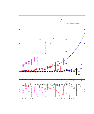
First, let us present our mass function fits. We use δc=1.46subscript𝛿𝑐1.46\delta_{c}=1.46 obtained by performing chisquare minimization together for H99, H500, F70, F122, F215 by forcing the same δcsubscript𝛿𝑐\delta_{c} but allowing overall rescaling factors (f2subscript𝑓2f_{2}) for each case. This is a reasonable procedure if one interprets shifting δcsubscript𝛿𝑐\delta_{c} as allowing departures from the assumption of spherical collapse, which should be relatively independent of the level of non-Gaussianity. However, the normalization requirement ρ¯=0MdndM𝑑M¯𝜌superscriptsubscript0𝑀𝑑𝑛𝑑𝑀differential-d𝑀\bar{\rho}=\int_{0}^{\infty}M\frac{dn}{dM}dM (which has not been analytically enforced) suggests that f2subscript𝑓2f_{2} should depend on the level of non-Gaussianity. The top panel of Figure 1 has our mass function results for two simulations with hierarchical scalings.
1234561014superscript101410^{14}1015superscript101510^{15}

nNGnGsubscript𝑛𝑁𝐺subscript𝑛𝐺\frac{n_{NG}}{n_{G}}

Mass (h1Msuperscript1subscript𝑀direct-producth^{-1}M_{\odot})H500, single field fNL=500subscript𝑓𝑁𝐿500f_{NL}=500Refer to captionz=0𝑧0z=0z=1𝑧1z=1z=2𝑧2z=2
11.522.531014superscript101410^{14}1015superscript101510^{15}

nNGnGsubscript𝑛𝑁𝐺subscript𝑛𝐺\frac{n_{NG}}{n_{G}}

Mass (h1Msuperscript1subscript𝑀direct-producth^{-1}M_{\odot})H99, single field fNL=99subscript𝑓𝑁𝐿99f_{NL}=99Refer to captionz=0𝑧0z=0z=1𝑧1z=1z=2𝑧2z=2
123456

nNGnGsubscript𝑛𝑁𝐺subscript𝑛𝐺\frac{n_{NG}}{n_{G}}

F215-0.5-0.3-0.10.11014superscript101410^{14}1015superscript101510^{15}Mass (h1Msuperscript1subscript𝑀direct-producth^{-1}M_{\odot})Refer to captionz=0𝑧0z=0z=1𝑧1z=1z=2𝑧2z=2
11.522.53

nNGnGsubscript𝑛𝑁𝐺subscript𝑛𝐺\frac{n_{NG}}{n_{G}}

F70-0.3-0.2-0.100.11014superscript101410^{14}1015superscript101510^{15}Mass (h1Msuperscript1subscript𝑀direct-producth^{-1}M_{\odot})Refer to captionz=0𝑧0z=0z=1𝑧1z=1z=2𝑧2z=2
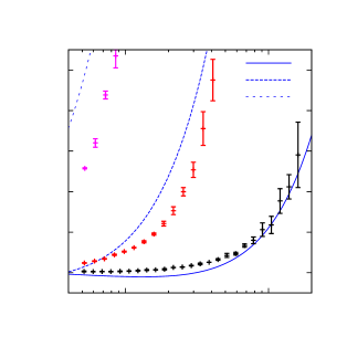
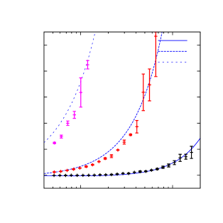
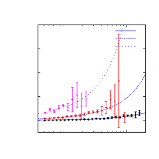
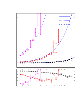
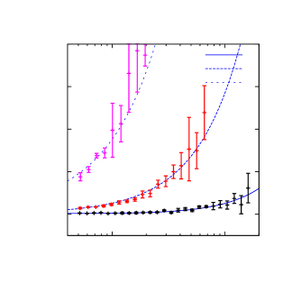
Figure 1: Top: the simulation results and semi-analytic prediction Eq.(5.2) for hierarchical simulations. Left panel: 3=0.145subscript30.145\mathcal{M}_{3}=0.145 (fNL=500subscript𝑓NL500f_{\rm NL}=500) with f2=1.042subscript𝑓21.042f_{2}=1.042. Right panel: 3=0.029subscript30.029\mathcal{M}_{3}=0.029 (fNL=99subscript𝑓NL99f_{\rm NL}=99) with f2=1.009subscript𝑓21.009f_{2}=1.009. Bottom: The simulation results and semi-analytic prediction Eq.(5.1) for feeder simulations. Left panel: 3=0.063subscript30.063\mathcal{M}_{3}=0.063 (fNLeff=215superscriptsubscript𝑓NLeff215f_{\rm NL}^{\rm eff}=215) and f2=1.043subscript𝑓21.043f_{2}=1.043. Right panel: 3=0.020subscript30.020\mathcal{M}_{3}=0.020 (fNLeff=70superscriptsubscript𝑓NLeff70f_{\rm NL}^{\rm eff}=70) with f2=1.012subscript𝑓21.012f_{2}=1.012. In addition, we also plot the fractional difference between the simulation results and the prediction from the truncated mass function Eq.(5.1) but using (δc=1.686,f2=1formulae-sequencesubscript𝛿𝑐1.686subscript𝑓21\delta_{c}=1.686,f_{2}=1), and assuming that nsubscript𝑛\mathcal{M}_{n} scale as Eq.(2.4). A negative value means that the analytic mass function overpredicts the simulation result.

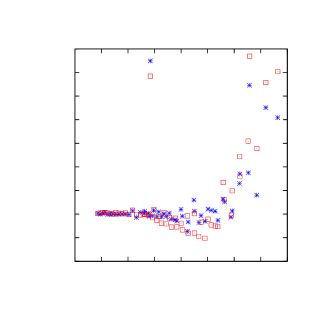
The results for two feeder simulations are presented in the bottom panels of Figure 1. As discussed in Appendix B, the errors on our truncated feeder mass function are large compared to the hierarchical case with comparable 3subscript3\mathcal{M}_{3}. Also, the error becomes large at relatively small ν𝜈\nu even for the feeder scaling case with 30.03subscript30.03\mathcal{M}_{3}\approx 0.03. Therefore, based on our error evaluation, we do not expect that our feeder mass function describes the simulation results well for the more massive halos or at higher redshifts for which νc3greater-than-or-equivalent-tosubscript𝜈𝑐3\nu_{c}\gtrsim 3. We find that the feeder mass function formula Eq.(5.1) fits well our simulation results for F70 and F122 (see the left panel of Figure 2 for the F122 simulation results). Consistent with the error analysis of feeder mass function, Eq.(5.1) fits to F215 with 30.063subscript30.063\mathcal{M}_{3}\approx 0.063 are not equally good. With a larger 30.198subscript30.198\mathcal{M}_{3}\approx 0.198, the F677 simulation is clearly not well fit by our truncated feeder mass function (see Figure 3). Finally, Figure 1 also shows the difference between the simulations and Eq.(5.1) assuming δc=1.686subscript𝛿𝑐1.686\delta_{c}=1.686, f2=1subscript𝑓21f_{2}=1, and that the moments scale exactly as in Eq.(2.4). That is, the bottom-most panels illustrate how calibrating on simulations shifts the purely analytic expectations for the non-Gaussian mass function. The dominant effect among these three factors is that of δcsubscript𝛿𝑐\delta_{c}; change in δcsubscript𝛿𝑐\delta_{c} affects the non-Gaussian mass functions starting at 𝒪(3)𝒪subscript3\mathcal{O}(\mathcal{M}_{3}). On the other hand, using different scalings of higher moments only change the expressions starting at 𝒪(4)𝒪subscript4\mathcal{O}(\mathcal{M}_{4}) and the f2subscript𝑓2f_{2} factors modify the mass functions at a few percent level at most (see Figure 4).

In Figure 2, the right hand panel shows the fractional difference between the semi-analytic expression Eq.(5.1) (with the cumulants nsubscript𝑛\mathcal{M}_{n} measured in the realizations and δcsubscript𝛿𝑐\delta_{c}, f2subscript𝑓2f_{2} fit) and the simulation results for the two feeder models: F122 and F215. We have plotted the fractional difference as a function of νc=δc/σMsubscript𝜈𝑐subscript𝛿𝑐subscript𝜎𝑀\nu_{c}=\delta_{c}/\sigma_{M} and the plotted points include simulation results from all three redshifts z=0,1,2𝑧012z=0,1,2. The result can be interpreted as the error in the semi-analytic approach and qualitatively correlates with our analytic error analysis of the PDF: (i) the error at low νcsubscript𝜈𝑐\nu_{c} is small, (ii) the error increases for higher νcsubscript𝜈𝑐\nu_{c} but the error is smaller for smaller 3subscript3\mathcal{M}_{3}.

On a different note, by looking at the non-Gaussian mass function results from simulations only, we can verify that the F70 model is more non-Gaussian than the H99 model (compare top and bottom plots in Figure 1), even though the skewness of F70 is smaller than the skewness of H99. Similarly, we also see that the F215 model has comparable amount of non-Gaussianity as the H500 model. This verifies that the non-Gaussian mass function is sensitive to the total non-Gaussianity and the scaling of higher moments in the initial conditions.
11.522.531014superscript101410^{14}1015superscript101510^{15}

nNGnGsubscript𝑛𝑁𝐺subscript𝑛𝐺\frac{n_{NG}}{n_{G}}

Mass (h1Msuperscript1subscript𝑀direct-producth^{-1}M_{\odot})F122Refer to captionz=0𝑧0z=0z=1𝑧1z=1z=2𝑧2z=2
-0.2-0.100.10.20.30.40.50.60.711.522.533.544.55

error

νcsubscript𝜈𝑐\nu_{c}Refer to captionF122F215
Figure 2: Left: the simulation results and the mass function prediction Eq.(5.1) for F122 model: 3=0.036subscript30.036\mathcal{M}_{3}=0.036 (fNLeff=122superscriptsubscript𝑓NLeff122f_{\rm NL}^{\rm eff}=122) with f2=1.021subscript𝑓21.021f_{2}=1.021. Right: the fractional error in the semi-analytic predictions for F215 and F122 models compared to simulation results. The plotted points include results from all three redshift values that we have looked at i.e. z=0,1,2𝑧012z=0,1,2.
1234561014superscript101410^{14}1015superscript101510^{15}

nNGnGsubscript𝑛𝑁𝐺subscript𝑛𝐺\frac{n_{NG}}{n_{G}}

Mass (h1Msuperscript1subscript𝑀direct-producth^{-1}M_{\odot})F677Refer to captionz=0𝑧0z=0z=1𝑧1z=1z=2𝑧2z=2
1234561014superscript101410^{14}1014superscript101410^{14}

nNGnGsubscript𝑛𝑁𝐺subscript𝑛𝐺\frac{n_{NG}}{n_{G}}

Mass (h1Msuperscript1subscript𝑀direct-producth^{-1}M_{\odot})M384Refer to captionz=0𝑧0z=0z=1𝑧1z=1z=2𝑧2z=2
Figure 3: The simulation results and semi-analytic mass function prediction for: (i) left: a feeder simulation with 30.198subscript30.198\mathcal{M}_{3}\approx 0.198 (f2=1.16subscript𝑓21.16f_{2}=1.16), and (ii) right: a mixed scaling simulation with 30.112subscript30.112\mathcal{M}_{3}\approx 0.112 (f2=1.06subscript𝑓21.06f_{2}=1.06).

The right hand panel of Figure 3 is a mixed scaling simulation with 3=0.112subscript30.112\mathcal{M}_{3}=0.112, and approximately a third of the contribution to the 3subscript3\mathcal{M}_{3} coming from the feeder component. For the theory curve we used both Eq.(5.1) and Eq.(5.2) for the corresponding 3subscript3\mathcal{M}_{3} components but forced the same f2subscript𝑓2f_{2}. As with the case with other simulations containing feeder scaling, the high νcsubscript𝜈𝑐\nu_{c} mass function results are not described well by the Edgeworth mass function.

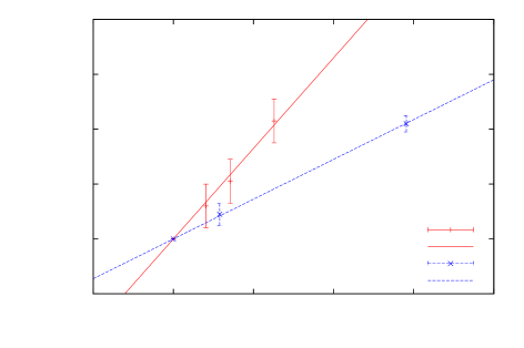
All in all, our analysis of the truncation error and the Edgeworth fits to the mass functions from simulations were qualitatively consistent with each other. Hence, we find that the error evaluation of the PDF is a good indicator of the accuracy of the Edgeworth (or Petrov) mass function. However, to fit the simulations well we needed to rescale the analytic ratio of non-Gaussian to Gaussian mass function by an extra 3subscript3\mathcal{M}_{3} dependent parameter, f2subscript𝑓2f_{2}, for both scalings. This rescaling seems reasonable to enforce the same total matter density regardless of level of non-Gaussianity. In Figure 4, we plot our best fit f2subscript𝑓2f_{2} values as a function of 3subscript3\mathcal{M}_{3} for both scalings. We find a simple linear relation between f2subscript𝑓2f_{2} and 3subscript3\mathcal{M}_{3}:

f2hiersuperscriptsubscript𝑓2hier\displaystyle f_{2}^{\rm hier} =\displaystyle= 1.0+0.2931.00.29subscript3\displaystyle 1.0+0.29\mathcal{M}_{3} (5.3)
f2feedsuperscriptsubscript𝑓2feed\displaystyle f_{2}^{\rm feed} =\displaystyle= 1.0+0.6631.00.66subscript3\displaystyle 1.0+0.66\mathcal{M}_{3} (5.4)
0.9811.021.041.061.08-0.0500.050.10.150.2

f2subscript𝑓2f_{2}

3subscript3\mathcal{M}_{3}Refer to captionfeeder1.0+0.6631.00.66subscript31.0+0.66\mathcal{M}_{3}hierarchical1.0+0.2931.00.29subscript31.0+0.29\mathcal{M}_{3}
Figure 4: 3subscript3\mathcal{M}_{3} dependence of f2subscript𝑓2f_{2} defined in Eq.(5.1) and Eq.(5.2) for feeder and hierarchical mass functions respectively. The data points are best fit f2subscript𝑓2f_{2} obtained from simulations and to obtain the best fit lines we require f2=0subscript𝑓20f_{2}=0 for 3=0subscript30\mathcal{M}_{3}=0.

3subscript3\mathcal{M}_{3}

hierarchicallog10(nNGnG)subscript10subscript𝑛𝑁𝐺subscript𝑛𝐺\log_{10}\left(\frac{n_{NG}}{n_{G}}\right)νcsubscript𝜈𝑐\nu_{c}Refer to caption
feederlog10(nNGnG)subscript10subscript𝑛𝑁𝐺subscript𝑛𝐺\log_{10}\left(\frac{n_{NG}}{n_{G}}\right)νcsubscript𝜈𝑐\nu_{c}Refer to caption
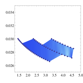
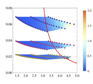
Figure 5: We plot results from our simulations for both hierarchical and feeder scalings as density plots. The quantity plotted is log10(nNG/nG)sim\log_{10}(n_{NG}/n_{G})_{\rm sim}. The points overlayed on the plots are the data points used to obtain the density plots. The red solid line shows the maximum trusted 3subscript3\mathcal{M}_{3} when allowing for 20% error in the PDF from νcsubscript𝜈𝑐\nu_{c} to some νc,maxsubscript𝜈𝑐𝑚𝑎𝑥\nu_{c,max}. The maximum trusted 3subscript3\mathcal{M}_{3} line for the hierarchical case lies outside of the plot range. See Appendix B for details of how these curves were obtained.

3subscript3\mathcal{M}_{3}

hierarchicalRSAsubscript𝑅𝑆𝐴R_{SA}νcsubscript𝜈𝑐\nu_{c}Refer to caption
feederRSAsubscript𝑅𝑆𝐴R_{SA}νcsubscript𝜈𝑐\nu_{c}Refer to caption
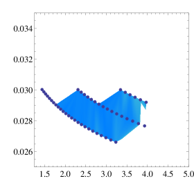
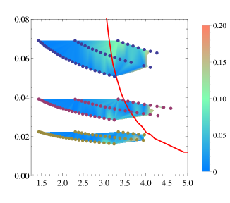
Figure 6: We plot the relative difference between the semi-analytic predictions (Eq.(5.2 or Eq.(5.1)) and the simulation results as a density plot. See Eq.(5.5) for the precise definition of the quantity plotted. We have omitted simulation results for which the uncertainty is larger than 20%percent2020\%. The important observation to note here is that the relative difference is quite small i.e. 0.2much-less-thanabsent0.2\ll 0.2, below the solid red line.

Analytic suggestions for non-Gaussian mass functions have also been obtained using excursion set methods [66, 67, 31, 68, 69, 70, 71]. It would be interesting to compare the predictions for additional corrections to Eq.(3.7) from those methods to these simulations, particularly the results for f2subscript𝑓2f_{2} shown in Figure 4.

To finish up our discussion of mass function results, in Figure 5 we show the non Gaussian mass function results (from simulations) in a two dimensional density plot on a νc3subscript𝜈𝑐subscript3\nu_{c}-\mathcal{M}_{3} plane, for both hierarchical and feeder scalings. We plot the quantity log10([nNG/nG]sim)subscript10subscriptdelimited-[]subscript𝑛𝑁𝐺subscript𝑛𝐺sim\log_{10}\left(\left[n_{NG}/n_{G}\right]_{\rm sim}\right). In the same plots, we overlay the maximum 3subscript3\mathcal{M}_{3} that we can trust the PDF 3.5, 3,maxsubscript3max\mathcal{M}_{3,\rm max}, as a function of νcsubscript𝜈𝑐\nu_{c}; see error analysis in Appendix B for details. In Figure 6, we have plots similar to those in Figure 5 but now we are plotting the relative difference of our mass function predictions (from 5.2 and 5.1) from the simulation results. The quantity plotted is:

RSAsubscript𝑅𝑆𝐴\displaystyle R_{SA} =\displaystyle= |(nNG/nG)sim(nNG/nG)semianalytic(nNG/nG)sim|subscriptsubscript𝑛𝑁𝐺subscript𝑛𝐺simsubscriptsubscript𝑛𝑁𝐺subscript𝑛𝐺semianalyticsubscriptsubscript𝑛𝑁𝐺subscript𝑛𝐺sim\displaystyle\left|\frac{(n_{NG}/n_{G})_{\rm sim}-(n_{NG}/n_{G})_{\rm semi-analytic}}{(n_{NG}/n_{G})_{\rm sim}}\right| (5.5)

These plots summarize our results for the mass function (for simulations with 3<0.08subscript30.08\mathcal{M}_{3}<0.08). Each isolated region in the density plots represents one simulation, which can be easily mapped to the exact simulation (in Table 1) by looking at the 3subscript3\mathcal{M}_{3} value. Figure 5 simply shows our simulation mass function results. But from Figure 6, we we can see that the magnitude of relative difference of our semi-analytic mass functions to the simulation results is generally less than ten percent (RSA0.1less-than-or-similar-tosubscript𝑅𝑆𝐴0.1R_{SA}\lesssim 0.1) for the values of νcsubscript𝜈𝑐\nu_{c} and 3subscript3\mathcal{M}_{3} that are calculated to be trustworthy by evaluating the series truncation error of the PDF 3.5. This is telling us that our semi-analytical mass function fits are consistent with the truncation error analysis.

Bias and Stochasticity:

Next we present simulation results and fit to the analytical predictions for large scale bias and large scale stochasticity. Before considering the non-Gaussian results, we present the results from our Gaussian simulations in Figure 7. Both the bias and the stochastic bias (after the 1/n¯1¯𝑛1/\bar{n} shot noise correction to Phh(k)subscript𝑃𝑘P_{hh}(k)) are constant for k<0.04hMpc1𝑘0.04superscriptMpc1k<0.04\;h\rm Mpc^{-1}, consistent with lowest order predictions for Gaussian fluctuations. Further, the large scale stochasticity parameter r2(k)superscript𝑟2𝑘r^{2}(k) is predicted to approach unity for Gaussian initial conditions. Figure 7 (right plot) is consistent with large scale stochasticity being constant for Gaussian initial conditions; however, the constant value is slightly greater than unity at rgaus2=1.03±0.02subscriptsuperscript𝑟2gausplus-or-minus1.030.02r^{2}_{\rm gaus}=1.03\pm 0.02 when halos in the mass range 4.83×10¹³h1MM9.55×1013h1M4.83superscript1013superscript1subscript𝑀direct-product𝑀9.55superscript1013superscript1subscript𝑀direct-product4.83\times 10^{13}h^{-1}M_{\odot}\leq M\leq 9.55\times 10^{13}h^{-1}M_{\odot} are used at z=0𝑧0z=0. For our other z=0𝑧0z=0 samples, the value of rgaus2subscriptsuperscript𝑟2gausr^{2}_{\rm gaus} increased when using halos of larger mass. The values of the fitted parameters (bias and stochasticity) for our Gaussian simulations are summarized in Table 2. We also note that the shot noise corrections are large for some of our halo samples. For example, the ratio of shot noise correction to the uncorrected halo power spectrum is largest for the halo sample at z=2𝑧2z=2 (Gaussian simulations) in Table 2; at a reference wavenumber k0.02hMpc1𝑘0.02superscriptMpc1k\approx 0.02\;h\rm Mpc^{-1}, this ratio is 0.8absent0.8\approx 0.8. Typically, this ratio is smaller (0.30.5absent0.30.5\approx 0.3-0.5) for the samples at smaller redshift in Table 2. Also, note that for many of our non-Gaussian models, the fractional shot noise contribution decreases to 0.3absent0.3\approx 0.3 even for the z=2𝑧2z=2 sample as there are more halos in the non-Gaussian samples at higher redshifts. Some progress has been made recently towards a better understanding and modeling of large scale stochasticity [72], beyond the usual shot noise correction, for Gaussian initial conditions. In this paper, however, we are focusing on the non-Gaussian effect only.

z𝑧z Mass range of halos used bgsubscript𝑏𝑔b_{g} rgaus2subscriptsuperscript𝑟2gausr^{2}_{\rm gaus}
0 (1.93M3.85)×1014h1M1.93𝑀3.85superscript1014superscript1subscript𝑀direct-product(1.93\leq M\leq 3.85)\times 10^{14}h^{-1}M_{\odot} 3.36±0.09plus-or-minus3.360.093.36\pm 0.09 1.13±0.06plus-or-minus1.130.061.13\pm 0.06
(0.965M1.92)×1014h1M0.965𝑀1.92superscript1014superscript1subscript𝑀direct-product(0.965\leq M\leq 1.92)\times 10^{14}h^{-1}M_{\odot} 2.57±0.04plus-or-minus2.570.042.57\pm 0.04 1.08±0.03plus-or-minus1.080.031.08\pm 0.03
(4.83M9.55)×1013h1M4.83𝑀9.55superscript1013superscript1subscript𝑀direct-product(4.83\leq M\leq 9.55)\times 10^{13}h^{-1}M_{\odot} 1.92±0.04plus-or-minus1.920.041.92\pm 0.04 1.03±0.02plus-or-minus1.030.021.03\pm 0.02
111 (0.965M1.92)×1014h1M0.965𝑀1.92superscript1014superscript1subscript𝑀direct-product(0.965\leq M\leq 1.92)\times 10^{14}h^{-1}M_{\odot} 5.83±0.24plus-or-minus5.830.245.83\pm 0.24 1.01±0.10plus-or-minus1.010.101.01\pm 0.10
(4.83M9.55)×1013h1M4.83𝑀9.55superscript1013superscript1subscript𝑀direct-product(4.83\leq M\leq 9.55)\times 10^{13}h^{-1}M_{\odot} 4.37±0.11plus-or-minus4.370.114.37\pm 0.11 1.04±0.05plus-or-minus1.040.051.04\pm 0.05
222 (4.83M9.55)×1013h1M4.83𝑀9.55superscript1013superscript1subscript𝑀direct-product(4.83\leq M\leq 9.55)\times 10^{13}h^{-1}M_{\odot} 8.68±0.44plus-or-minus8.680.448.68\pm 0.44 0.84±0.29plus-or-minus0.840.290.84\pm 0.29
Table 2: Large scale bias and stochasticity for simulations with Gaussian initial conditions. Simple chisquare fitting was performed to obtain the best fit values. The errors in bgsubscript𝑏𝑔b_{g} and r2(k)superscript𝑟2𝑘r^{2}(k) are computed such that the reduced chisquare increases by unity when adding the error to the best fit values. We will use the same procedure to obtain best fit values and the corresponding error for our non-Gaussian bias and stochasticity results.
1.522.533.544.555.50.01

bias

k(hMpc1)𝑘superscriptMpc1k\;(h\;\rm Mpc^{-1})GuassianRefer to captionz=1z=0
0.80.911.11.2

r2(k)superscript𝑟2𝑘r^{2}(k)

Gaussian0.80.911.11.20.01

r2(k)superscript𝑟2𝑘r^{2}(k)

k(hMpc1)𝑘superscriptMpc1k\;(h\;\rm Mpc^{-1})Refer to captionz=1z=0
Figure 7: The bias (left) and stochasticity (right) at large scales for the Gaussian simulations at z=0𝑧0z=0 and z=1𝑧1z=1 using halos in the mass range 4.83×10¹³h1MM9.55×1013h1M4.83superscript1013superscript1subscript𝑀direct-product𝑀9.55superscript1013superscript1subscript𝑀direct-product4.83\times 10^{13}h^{-1}M_{\odot}\leq M\leq 9.55\times 10^{13}h^{-1}M_{\odot}. The values of large scale Gaussian bias and stochastic bias obtained through the fits can be found in Table 2.
1.522.533.544.550.01

bias

k(hMpc1)𝑘superscriptMpc1k\;(h\;\rm Mpc^{-1})single field, z=0Refer to captionH500, using bgsubscript𝑏𝑔b_{g}H500, using bψsubscript𝑏𝜓b_{\psi}H99, using bgsubscript𝑏𝑔b_{g}H99, using bψsubscript𝑏𝜓b_{\psi}
0.80.911.11.2

r2(k)superscript𝑟2𝑘r^{2}(k)

single field0.80.911.11.20.01

r2(k)superscript𝑟2𝑘r^{2}(k)

k(hMpc1)𝑘superscriptMpc1k\;(h\;\rm Mpc^{-1})Refer to captionH500H99
Figure 8: Left: the simulation result for bias Phm/Pmmsubscript𝑃𝑚subscript𝑃𝑚𝑚P_{hm}/P_{mm} at large scales for the hierarchical simulations at z=0𝑧0z=0 using halos in the mass range 9.65×10¹³h1MM1.92×1014h1M9.65superscript1013superscript1subscript𝑀direct-product𝑀1.92superscript1014superscript1subscript𝑀direct-product9.65\times 10^{13}h^{-1}M_{\odot}\leq M\leq 1.92\times 10^{14}h^{-1}M_{\odot} and the corresponding best fit using Eq.(LABEL:eq:hmbiasfinal). For each set of simulation data, we also include the curve obtained by using bgsubscript𝑏𝑔b_{g} from Gaussian simulation instead of the fitted bψsubscript𝑏𝜓b_{\psi}. For the case of H500 shown in the figure, bψ=1.86±0.03subscript𝑏𝜓plus-or-minus1.860.03b_{\psi}=1.86\pm 0.03 compared to bg=1.92±0.04subscript𝑏𝑔plus-or-minus1.920.04b_{g}=1.92\pm 0.04. Right: the corresponding large scale stochasticity simulation results Eq.(3.13) and the best fit constant values.

We have derived expressions for Phm(k)subscript𝑃𝑚𝑘P_{hm}(k) and Phh(k)subscript𝑃𝑘P_{hh}(k) for our two source model in Appendix C. These expressions written in terms of the total matter power spectrum Pmm(k)=α(k)2PΦ(k)subscript𝑃𝑚𝑚𝑘𝛼superscript𝑘2subscript𝑃Φ𝑘P_{mm}(k)=\alpha(k)^{2}P_{\Phi}(k) and the constant halo bias coefficients (bϕsubscript𝑏italic-ϕb_{\phi} and bψsubscript𝑏𝜓b_{\psi}) for the two independent fields ϕitalic-ϕ\phi and ψ𝜓\psi are:

Phm(k)Pmm(k)subscript𝑃𝑚𝑘subscript𝑃𝑚𝑚𝑘\displaystyle\frac{P_{hm}(k)}{P_{mm}(k)} =\displaystyle= bϕ(1q)1+f~NL2I1(k)q𝒫ψ,G+(bψ+2δc(bψ1)f~NLα(k)σR,ψ2σR2)(q+f~NL2I1(k)q𝒫ψ,G(k)1+f~NL2I1(k)q𝒫ψ,G)subscript𝑏italic-ϕ1𝑞1superscriptsubscript~𝑓NL2subscript𝐼1𝑘𝑞subscript𝒫𝜓𝐺subscript𝑏𝜓2subscript𝛿𝑐subscript𝑏𝜓1subscript~𝑓NL𝛼𝑘superscriptsubscript𝜎𝑅𝜓2superscriptsubscript𝜎𝑅2𝑞superscriptsubscript~𝑓NL2subscript𝐼1𝑘𝑞subscript𝒫𝜓𝐺𝑘1superscriptsubscript~𝑓NL2subscript𝐼1𝑘𝑞subscript𝒫𝜓𝐺\displaystyle\frac{b_{\phi}(1-q)}{1+\tilde{f}_{\rm NL}^{2}I_{1}(k)q\mathcal{P}_{\psi,G}}+\left(b_{\psi}+2\delta_{c}(b_{\psi}-1)\frac{\tilde{f}_{\rm NL}}{\alpha(k)}\frac{\sigma_{R,\psi}^{2}}{\sigma_{R}^{2}}\right)\left(\frac{q+\tilde{f}_{\rm NL}^{2}I_{1}(k)q\mathcal{P}_{\psi,G}(k)}{1+\tilde{f}_{\rm NL}^{2}I_{1}(k)q\mathcal{P}_{\psi,G}}\right)\;

and,

Phh(k)Pmm(k)subscript𝑃𝑘subscript𝑃𝑚𝑚𝑘\displaystyle\frac{P_{hh}(k)}{P_{mm}(k)} =\displaystyle= bϕ2(1q)1+f~NL2I1(k)q𝒫ψ,G+(bψ+2δc(bψ1)f~NLα(k)σR,ψ2σR2)2(q+f~NL2I1(k)q𝒫ψ,G(k)1+f~NL2I1(k)q𝒫ψ,G)superscriptsubscript𝑏italic-ϕ21𝑞1superscriptsubscript~𝑓NL2subscript𝐼1𝑘𝑞subscript𝒫𝜓𝐺superscriptsubscript𝑏𝜓2subscript𝛿𝑐subscript𝑏𝜓1subscript~𝑓NL𝛼𝑘superscriptsubscript𝜎𝑅𝜓2superscriptsubscript𝜎𝑅22𝑞superscriptsubscript~𝑓NL2subscript𝐼1𝑘𝑞subscript𝒫𝜓𝐺𝑘1superscriptsubscript~𝑓NL2subscript𝐼1𝑘𝑞subscript𝒫𝜓𝐺\displaystyle\frac{b_{\phi}^{2}(1-q)}{1+\tilde{f}_{\rm NL}^{2}I_{1}(k)q\mathcal{P}_{\psi,G}}+\left(b_{\psi}+2\delta_{c}(b_{\psi}-1)\frac{\tilde{f}_{\rm NL}}{\alpha(k)}\frac{\sigma_{R,\psi}^{2}}{\sigma_{R}^{2}}\right)^{2}\left(\frac{q+\tilde{f}_{\rm NL}^{2}I_{1}(k)q\mathcal{P}_{\psi,G}(k)}{1+\tilde{f}_{\rm NL}^{2}I_{1}(k)q\mathcal{P}_{\psi,G}}\right)\;

For each model (listed in Table 1) we have measured the auto and cross correlations in the matter and halo fields, using halos in the same mass bins and redshifts shown in Table 2. To check how well the analytic expressions above fit the simulation results, we measured the bias coefficients bϕsubscript𝑏italic-ϕb_{\phi} and bψsubscript𝑏𝜓b_{\psi} for each case by cross-correlating the halo density field for each sample with (i) the ϕG(x)subscriptitalic-ϕ𝐺𝑥\phi_{G}(\vec{x}) part of the linear density field, and (ii) the ψG(x)+f~NLψG(x)2subscript𝜓𝐺𝑥subscript~𝑓NLsubscript𝜓𝐺superscript𝑥2\psi_{G}(\vec{x})+\tilde{f}_{\rm NL}\psi_{G}(\vec{x})^{2} part of the linear density field. For the correlation with the Gaussian field, we expect a constant large scale bias bϕsubscript𝑏italic-ϕb_{\phi}. For the second case we expect a scale-independent piece and a scale dependent term. The expression for this bias is obtained using Eq.(C.6) by cross correlating δhsubscript𝛿\delta_{h} and δψ,NGsubscript𝛿𝜓NG\delta_{\psi,\rm NG}, to get:

PhψPψψsubscript𝑃𝜓subscript𝑃𝜓𝜓\displaystyle\frac{P_{h\psi}}{P_{\psi\psi}} =\displaystyle= bψ+2δc(bψ1)f~NLα(k)σR,ψ2σR2subscript𝑏𝜓2subscript𝛿𝑐subscript𝑏𝜓1subscript~𝑓NL𝛼𝑘superscriptsubscript𝜎𝑅𝜓2superscriptsubscript𝜎𝑅2\displaystyle b_{\psi}+\frac{2\delta_{c}(b_{\psi}-1)\tilde{f}_{\rm NL}}{\alpha(k)}\frac{\sigma_{R,\psi}^{2}}{\sigma_{R}^{2}} (5.8)

Equations (LABEL:eq:hmbiasfinal) and (LABEL:eq:hhbiasfinal) clearly give the expected result for the Gaussian case in the q=0𝑞0q=0 limit; in this case only the ϕitalic-ϕ\phi field contributes to the initial density field. We obtain the single field non-Gaussian (hierarchical, feeder, or mixed) limit for q=1𝑞1q=1, in which case there is no contribution from the ϕitalic-ϕ\phi field to the initial density field. Further, in case of single field hierarchical models,

(1+f~NL2𝒫ψ,G(k)I1(k)1+f~NL2q𝒫ψ,G(k)I1(k))1superscriptsubscript~𝑓NL2subscript𝒫𝜓𝐺𝑘subscript𝐼1𝑘1superscriptsubscript~𝑓NL2𝑞subscript𝒫𝜓𝐺𝑘subscript𝐼1𝑘\displaystyle\left(\frac{1+\tilde{f}_{\rm NL}^{2}\mathcal{P}_{\psi,G}(k)I_{1}(k)}{1+\tilde{f}_{\rm NL}^{2}q\mathcal{P}_{\psi,G}(k)I_{1}(k)}\right) =\displaystyle= 1,andσR,ψ2σR2q1andsuperscriptsubscript𝜎𝑅𝜓2superscriptsubscript𝜎𝑅2𝑞\displaystyle 1\;,{\rm and}\;\frac{\sigma_{R,\psi}^{2}}{\sigma_{R}^{2}}\approx q (5.9)

and we recover the known results for the local ansatz. Using the general expressions in Eq.(LABEL:eq:hmbiasfinal) and Eq.(LABEL:eq:hhbiasfinal) and the best fit bias parameters for each source field, we will compare the semi-analytical predictions for the bias and the stochasticity parameter r2(k)superscript𝑟2𝑘r^{2}(k) to our simulation results.

1101000.01

bias

k(hMpc1)𝑘superscriptMpc1k\;(h\;\rm Mpc^{-1})F677Refer to captionz=0z=1z=2
00.20.40.60.810.01

r2(k)superscript𝑟2𝑘r^{2}(k)

k(hMpc1)𝑘superscriptMpc1k\;(h\;\rm Mpc^{-1})F677Refer to captionz=0z=1z=2
1101000.01

bias

k(hMpc1)𝑘superscriptMpc1k\;(h\;\rm Mpc^{-1})F215Refer to captionz=0z=1z=2
00.20.40.60.811.20.01

r2(k)superscript𝑟2𝑘r^{2}(k)

k(hMpc1)𝑘superscriptMpc1k\;(h\;\rm Mpc^{-1})F215Refer to captionz=0z=1z=2
Figure 9: Top: the bias Phm/Pmmsubscript𝑃𝑚subscript𝑃𝑚𝑚P_{hm}/P_{mm} (left) and stochasticity r2(k)superscript𝑟2𝑘r^{2}(k) (right) at large scales for the feeder simulation F677 at z=0,1,2𝑧012z=0,1,2 using halos in the mass range 4.83×10¹³h1MM9.55×1013h1M4.83superscript1013superscript1subscript𝑀direct-product𝑀9.55superscript1013superscript1subscript𝑀direct-product4.83\times 10^{13}h^{-1}M_{\odot}\leq M\leq 9.55\times 10^{13}h^{-1}M_{\odot}. The analytical curves for the bias is obtained using Eq.(LABEL:eq:hmbiasfinal) for which the bias coefficients bψsubscript𝑏𝜓b_{\psi} and bϕsubscript𝑏italic-ϕb_{\phi} are measured by cross-correlating each halo sample with the linear density field contribution from the ϕitalic-ϕ\phi and ψ𝜓\psi fields respectively. The analytical curves for the stochasticity is obtained using Eq.(LABEL:eq:hmbiasfinal) and Eq.(LABEL:eq:hhbiasfinal) in Eq.(3.13) using the same bϕsubscript𝑏italic-ϕb_{\phi} and the same bψsubscript𝑏𝜓b_{\psi} as the corresponding bias curve on the left plot. Bottom: same as top but for the model F215 using the same halo samples. All the analytical curves for the bias are consistent with the simulation results. For the stochasticity r2(k)superscript𝑟2𝑘r^{2}(k), the most discrepant case in the above plots (the F677, z=0𝑧0z=0 sample) is off by about five percent.

Now, let us discuss the single field hierarchical scenario first. Note that we use δc=1.46subscript𝛿𝑐1.46\delta_{c}=1.46, the best fit δcsubscript𝛿𝑐\delta_{c} from our mass function fits. We find that a different best fit bψsubscript𝑏𝜓b_{\psi} is preferred compared to the corresponding Gaussian bias bgsubscript𝑏𝑔b_{g} measured from Gaussian simulations. This can be clearly seen in Figure 8, especially in the case of H500. We checked this to be true for other halo samples listed in Table 2. In general, we find the best fit bψsubscript𝑏𝜓b_{\psi} is less than the corresponding bgsubscript𝑏𝑔b_{g}; this is consistent with the picture that bias decreases as mass function increases [73]. From Figure 8 (right plot), we can also verify that the single field non-Gaussian cases do not produce excess stochasticity than the Gaussian case as predicted. For the two more massive halos samples at z=0𝑧0z=0, for which the Gaussian stochasticity itself deviates from unity, we find similar level of deviation from unity in the non-Gaussian case.

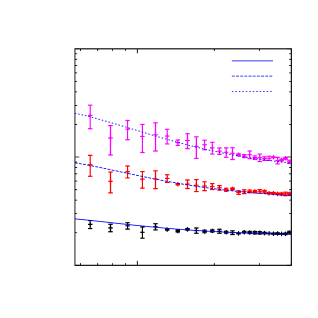
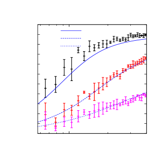
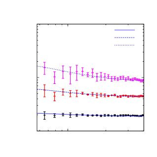
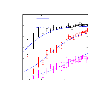
In Figure 9, we show bias and stochasticity results for two of our feeder cases. We find that for the cases in which the corresponding rgaus2subscriptsuperscript𝑟2gausr^{2}_{\rm gaus} is consistent with unity, the simulation results for the stochasticity are described quite well by the analytic expression. In Figure 10, we show another example of a feeder case F70 and an example for a mixed case M997. In Table 3, we list the values bψsubscript𝑏𝜓b_{\psi} and bϕsubscript𝑏italic-ϕb_{\phi} used in the plots.

1101000.01

bias

k(hMpc1)𝑘superscriptMpc1k\;(h\;\rm Mpc^{-1})F70Refer to captionz=0z=1z=2
00.20.40.60.811.20.01

r2(k)superscript𝑟2𝑘r^{2}(k)

k(hMpc1)𝑘superscriptMpc1k\;(h\;\rm Mpc^{-1})F70Refer to captionz=0z=1z=2
1101000.01

bias

k(hMpc1)𝑘superscriptMpc1k\;(h\;\rm Mpc^{-1})M997Refer to captionz=0z=1z=2
00.20.40.60.810.01

r2(k)superscript𝑟2𝑘r^{2}(k)

k(hMpc1)𝑘superscriptMpc1k\;(h\;\rm Mpc^{-1})M997Refer to captionz=0z=1z=2
Figure 10: Top: the bias Phm/Pmmsubscript𝑃𝑚subscript𝑃𝑚𝑚P_{hm}/P_{mm} (left) and stochasticity r2(k)superscript𝑟2𝑘r^{2}(k) (right) at large scales for the feeder simulation F70 at z=0,1,2𝑧012z=0,1,2 using halos in the mass range 4.83×10¹³h1MM9.55×1013h1M4.83superscript1013superscript1subscript𝑀direct-product𝑀9.55superscript1013superscript1subscript𝑀direct-product4.83\times 10^{13}h^{-1}M_{\odot}\leq M\leq 9.55\times 10^{13}h^{-1}M_{\odot}. The analytical curves for the bias are obtained using Eq.(LABEL:eq:hmbiasfinal) for which the bias coefficients bψsubscript𝑏𝜓b_{\psi} and bϕsubscript𝑏italic-ϕb_{\phi} are measured by cross-correlating each halo sample with the linear density field contribution from the ϕitalic-ϕ\phi and ψ𝜓\psi fields respectively. The analytical curves for the stochasticity are obtained using Eq.(LABEL:eq:hmbiasfinal) and Eq.(LABEL:eq:hhbiasfinal) in Eq.(3.13) using the same bϕsubscript𝑏italic-ϕb_{\phi} and the same bψsubscript𝑏𝜓b_{\psi} as the corresponding bias curve on the left plot. Bottom: same as top but for the model M997 using the same halo samples.
z=0 z=1 z=2
bϕsubscript𝑏italic-ϕb_{\phi} bψsubscript𝑏𝜓b_{\psi} bϕsubscript𝑏italic-ϕb_{\phi} bψsubscript𝑏𝜓b_{\psi} bϕsubscript𝑏italic-ϕb_{\phi} bψsubscript𝑏𝜓b_{\psi}
F677 1.76±0.05plus-or-minus1.760.051.76\pm 0.05 1.85±0.05plus-or-minus1.850.051.85\pm 0.05 3.34±0.19plus-or-minus3.340.193.34\pm 0.19 4.15±0.09plus-or-minus4.150.094.15\pm 0.09 4.49±0.31plus-or-minus4.490.314.49\pm 0.31 9.24±0.17plus-or-minus9.240.179.24\pm 0.17
F215 1.83±0.05plus-or-minus1.830.051.83\pm 0.05 2.08±0.13plus-or-minus2.080.132.08\pm 0.13 3.96±0.14plus-or-minus3.960.143.96\pm 0.14 5.04±0.10plus-or-minus5.040.105.04\pm 0.10 6.36±0.63plus-or-minus6.360.636.36\pm 0.63 14.36±0.48plus-or-minus14.360.4814.36\pm 0.48
F70 1.88±0.04plus-or-minus1.880.041.88\pm 0.04 2.25±0.23plus-or-minus2.250.232.25\pm 0.23 4.18±0.11plus-or-minus4.180.114.18\pm 0.11 5.09±0.23plus-or-minus5.090.235.09\pm 0.23 7.88±0.55plus-or-minus7.880.557.88\pm 0.55 15.08±0.96plus-or-minus15.080.9615.08\pm 0.96
M997 1.87±0.08plus-or-minus1.870.081.87\pm 0.08 1.95±0.06plus-or-minus1.950.061.95\pm 0.06 2.95±0.09plus-or-minus2.950.092.95\pm 0.09 3.83±0.06plus-or-minus3.830.063.83\pm 0.06 4.16±0.46plus-or-minus4.160.464.16\pm 0.46 7.18±0.11plus-or-minus7.180.117.18\pm 0.11
Table 3: Values of the bias coefficients bϕsubscript𝑏italic-ϕb_{\phi} and bψsubscript𝑏𝜓b_{\psi} measured by cross correlating the halo density field with the corresponding ϕitalic-ϕ\phi and ψ𝜓\psi components in the linear density field. In all redshifts z=0,1,2𝑧012z=0,1,2 listed above, the mass range for the halo samples used was 4.83×10¹³h1MM9.55×1013h1M4.83superscript1013superscript1subscript𝑀direct-product𝑀9.55superscript1013superscript1subscript𝑀direct-product4.83\times 10^{13}h^{-1}M_{\odot}\leq M\leq 9.55\times 10^{13}h^{-1}M_{\odot}. These same halo samples are used for the bias and stochasticity plots shown in Figures 9 and 10.

We have only shown bias and stochasticity results for three samples out of the six samples listed in Table 2. Let us comment on the results obtained for the samples for which results are not presented here. First, we find that the bias Phm/Pmmsubscript𝑃𝑚subscript𝑃𝑚𝑚P_{hm}/P_{mm} results agree with the analytic prediction for all the samples. Similarly, the stochasticity r2(k)superscript𝑟2𝑘r^{2}(k) for the z=1𝑧1z=1 sample with mass range 9.65×10¹³h1MM1.92×1014h1M9.65superscript1013superscript1subscript𝑀direct-product𝑀1.92superscript1014superscript1subscript𝑀direct-product9.65\times 10^{13}h^{-1}M_{\odot}\leq M\leq 1.92\times 10^{14}h^{-1}M_{\odot} has excellent fits to the simulation data for all the feeder and mixed models. However, we find that the stochasticity r2(k)superscript𝑟2𝑘r^{2}(k) results for the two samples at z=0𝑧0z=0 with mass ranges: (i) (0.965M1.92)×1014h1M0.965𝑀1.92superscript1014superscript1subscript𝑀direct-product(0.965\leq M\leq 1.92)\times 10^{14}h^{-1}M_{\odot} and (ii) (1.93M3.85)×1014h1M1.93𝑀3.85superscript1014superscript1subscript𝑀direct-product(1.93\leq M\leq 3.85)\times 10^{14}h^{-1}M_{\odot} show deviations from the analytic predictions, roughly at the same level as the deviation shown by corresponding Gaussian rgaus2subscriptsuperscript𝑟2gausr^{2}_{\rm gaus} from unity (at 10%absentpercent10\approx 10\% level).

Reference [62] found that the stochastic bias predictions for one case of a two field model were off by roughly a factor of 0.70.70.7. For comparison, we define their b0subscript𝑏0b_{0} in our notation:

b0subscript𝑏0\displaystyle b_{0} =\displaystyle= (1q)bϕ+qbψ1+f~NL2q𝒫ψ,G(k)I1(k)1𝑞subscript𝑏italic-ϕ𝑞subscript𝑏𝜓1superscriptsubscript~𝑓NL2𝑞subscript𝒫𝜓𝐺𝑘subscript𝐼1𝑘\displaystyle\frac{(1-q)b_{\phi}+qb_{\psi}}{1+\tilde{f}_{\rm NL}^{2}q\mathcal{P}_{\psi,G}(k)I_{1}(k)} (5.10)

For their particular model, b012(bϕ+bψ)subscript𝑏012subscript𝑏italic-ϕsubscript𝑏𝜓b_{0}\approx\frac{1}{2}(b_{\phi}+b_{\psi}), and their model assumes b0=bϕ=bψsubscript𝑏0subscript𝑏italic-ϕsubscript𝑏𝜓b_{0}=b_{\phi}=b_{\psi}. However, our results indicate that we may have to relax this assumption in general two source non-Gaussian scenarios. We expect better match between simulation results and peak background split calculation in their work too, once bψsubscript𝑏𝜓b_{\psi} and bϕsubscript𝑏italic-ϕb_{\phi} are measured separately, in addition to accounting for the 𝒪(f~NL3)𝒪superscriptsubscript~𝑓NL3\mathcal{O}(\tilde{f}_{\rm NL}^{3}) term in the bispectrum, and the 𝒪(f~NL4)𝒪superscriptsubscript~𝑓NL4\mathcal{O}(\tilde{f}_{\rm NL}^{4}) term in the trispectrum.

6 Conclusion

In this paper, we have reported results for the mass function of massive halos and scale dependent bias from N-body simulations using a generalized two field model of primordial non-Gaussianity. The two field ansatz is used to generate initial conditions where the higher moments nsubscript𝑛\mathcal{M}_{n}, n>3𝑛3n>3 are more important than in the standard local ansatz, given the same value of 3subscript3\mathcal{M}_{3} as the single field local ansatz case. That this can be done is not mathematically surprising, but we have considered a range of scalings that are very natural from particle physics models of inflation. We have shown that in using large scale structure data to constrain the primordial fluctuations, assumptions about the scaling of higher moments should be explicitly stated. In addition, we have shown that in scenarios with more than one source for the density fluctuations it is important to allow independent bias coefficients for each source.

Our simulations show that the Petrov expansion gives a good approximation to the non-Gaussian mass function when the amount of non-Gaussianity is small enough. The criteria for “small enough” depends on the dimensionless skewness 3subscript3\mathcal{M}_{3} and the scaling of moments. We have verified that for the same level of skewness, the feeder scaling is more non-Gaussian than the hierarchical scaling by a straightforward comparison of simulation outputs of the two cases. For the parameter space we probed, we were able to show that the truncation error evaluation of the Petrov PDF, Eq.(3.5), correlated well with the degree to which the truncated non-Gaussian mass function fitted the simulation results. This gives us further confidence in the use of the truncated Petrov (Edgeworth) mass function for various analyses such as that of [74, 13] to put constraints on primordial non-Gaussianity using number counts of objects. We make progress towards calibrating the mass function formulae Eq.(5.2) and Eq.(5.1) for both scalings by using an extra parameter f2subscript𝑓2f_{2}, in addition to verifying that a reduced δcsubscript𝛿𝑐\delta_{c} is preferred, which is consistent with previous simulation studies of non-Gaussian mass functions with non-Gaussianity of local type and hierarchical scaling of higher moments. The effect this calibration might have on previous analysis of cluster constraints is illustrated in the bottom panels of Figure 1.

Similarly, the peak-background-split calculations are good fits to the non-Gaussian bias results (Phm(k)/Pmm(k)subscript𝑃𝑚𝑘subscript𝑃𝑚𝑚𝑘P_{hm}(k)/P_{mm}(k)) from simulations—both for the hierarchical models (previously done a number of times) and for the feeder models. Moreover, we also presented results for large scale stochastic bias from our simulations which, in addition to the halo-matter bias, also depends on Phh(k)/Pmm(k)subscript𝑃𝑘subscript𝑃𝑚𝑚𝑘P_{hh}(k)/P_{mm}(k). We found that, for two source scenarios, both the bias and stochastic bias calculations work well once we allow for different bias coefficients for the two independent fields. These bias coefficients, namely bϕsubscript𝑏italic-ϕb_{\phi} and bψsubscript𝑏𝜓b_{\psi} in our notation, were measured by cross-correlating the halo density field with the linear density field contributions from ϕitalic-ϕ\phi and ψ𝜓\psi fields separately. The analytical calculations deviated from the simulation results for the stochastic bias only for halo samples whose values of stochasticity were inconsistent with unity in the Gaussian simulations. Therefore, for these halo samples, we expect the need to account for other contributions to the stochasticity that have to be taken into account even in the Gaussian case. While we have not investigated this issue in detail, additional studies would be worthwhile since a better understanding of stochasticity is useful for cosmological applications of galaxy surveys.

Acknowledgment:

This work is supported by the National Aeronautics and Space Administration under Grant No. NNX12AC99G issued through the Astrophysics Theory Program. This work used the Extreme Science and Engineering Discovery Environment (XSEDE), which is supported by National Science Foundation grant number OCI-1053575. The simulations for the project were performed using computing resources at the Texas Advanced Computing Center (TACC), The University of Texas at Austin through XSEDE grant AST130053 and at the Penn State Research Computing and Cyberinfrastructure (RCC). S. A. would like to thank Xinghai Zhao for suggestions on setting up Gadget simulations.

Appendix A Integrals for δRncsubscriptdelimited-⟨⟩superscriptsubscript𝛿𝑅𝑛𝑐\langle\delta_{R}^{n}\rangle_{c}

Here we list some of the integrals for δRnc=δRn1+δRn2subscriptdelimited-⟨⟩superscriptsubscript𝛿𝑅𝑛𝑐subscriptdelimited-⟨⟩superscriptsubscript𝛿𝑅𝑛1subscriptdelimited-⟨⟩superscriptsubscript𝛿𝑅𝑛2\langle\delta_{R}^{n}\rangle_{c}=\langle\delta_{R}^{n}\rangle_{1}+\langle\delta_{R}^{n}\rangle_{2}, where the subscripts 111 and 222 are for the 𝒪(f~NLn2\mathcal{O}(\tilde{f}_{\rm NL}^{n-2}) and 𝒪(f~NLn\mathcal{O}(\tilde{f}_{\rm NL}^{n}) terms respectively.

δR21subscriptdelimited-⟨⟩superscriptsubscript𝛿𝑅21\displaystyle\langle\delta_{R}^{2}\rangle_{1} =\displaystyle= 1qd3k(2π)3α(k)2WR(k)2Pψ(k)=1qdkkα(k)2WR(k)2𝒫ψ(k)1𝑞superscript𝑑3𝑘superscript2𝜋3𝛼superscript𝑘2subscript𝑊𝑅superscript𝑘2subscript𝑃𝜓𝑘1𝑞𝑑𝑘𝑘𝛼superscript𝑘2subscript𝑊𝑅superscript𝑘2subscript𝒫𝜓𝑘\displaystyle\frac{1}{q}\int\frac{d^{3}\vec{k}}{(2\pi)^{3}}\alpha(k)^{2}W_{R}(k)^{2}P_{\psi}(k)=\frac{1}{q}\int\frac{dk}{k}\alpha(k)^{2}W_{R}(k)^{2}\mathcal{P}_{\psi}(k) (A.1)
δR22subscriptdelimited-⟨⟩superscriptsubscript𝛿𝑅22\displaystyle\langle\delta_{R}^{2}\rangle_{2} =\displaystyle= 2f~NL2d3k(2π)3d3p(2π)3α(k)2WR(k)2Pψ(p)Pψ(|pk|)2superscriptsubscript~𝑓NL2superscript𝑑3𝑘superscript2𝜋3superscript𝑑3𝑝superscript2𝜋3𝛼superscript𝑘2subscript𝑊𝑅superscript𝑘2subscript𝑃𝜓𝑝subscript𝑃𝜓𝑝𝑘\displaystyle 2\tilde{f}_{\rm NL}^{2}\int\frac{d^{3}\vec{k}}{(2\pi)^{3}}\int\frac{d^{3}\vec{p}}{(2\pi)^{3}}\alpha(k)^{2}W_{R}(k)^{2}P_{\psi}(p)P_{\psi}(|\vec{p}-\vec{k}|) (A.2)
=\displaystyle= f~NL2k2𝑑k𝑑p11𝑑μ[α(k)2WR(k)2𝒫ψ(p)𝒫ψ(|pk|)p|pk|3]superscriptsubscript~𝑓NL2superscript𝑘2differential-d𝑘differential-d𝑝superscriptsubscript11differential-d𝜇delimited-[]𝛼superscript𝑘2subscript𝑊𝑅superscript𝑘2subscript𝒫𝜓𝑝subscript𝒫𝜓𝑝𝑘𝑝superscript𝑝𝑘3\displaystyle\tilde{f}_{\rm NL}^{2}\int k^{2}dk\int dp\int_{-1}^{1}d\mu\left[\alpha(k)^{2}W_{R}(k)^{2}\frac{\mathcal{P}_{\psi}(p)\mathcal{P}_{\psi}(|\vec{p}-\vec{k}|)}{p|\vec{p}-\vec{k}|^{3}}\right]

The δR3delimited-⟨⟩superscriptsubscript𝛿𝑅3\langle\delta_{R}^{3}\rangle terms are:

δR31subscriptdelimited-⟨⟩superscriptsubscript𝛿𝑅31\displaystyle\langle\delta_{R}^{3}\rangle_{1} =\displaystyle= 6f~NLd3k1(2π)3d3k2(2π)3(αW)1,2,12Pψ(k1)Pψ(k2)6subscript~𝑓NLsuperscript𝑑3subscript𝑘1superscript2𝜋3superscript𝑑3subscript𝑘2superscript2𝜋3subscript𝛼𝑊1212subscript𝑃𝜓subscript𝑘1subscript𝑃𝜓subscript𝑘2\displaystyle 6\tilde{f}_{\rm NL}\int\frac{d^{3}\vec{k_{1}}}{(2\pi)^{3}}\int\frac{d^{3}\vec{k_{2}}}{(2\pi)^{3}}(\alpha W)_{1,2,12}P_{\psi}(k_{1})P_{\psi}(k_{2}) (A.3)
=\displaystyle= 6f~NL[12dk1k1dk2k211𝑑μ[(αW)1,2,12𝒫ψ(k1)𝒫ψ(k2)]]6subscript~𝑓NLdelimited-[]12𝑑subscript𝑘1subscript𝑘1𝑑subscript𝑘2subscript𝑘2superscriptsubscript11differential-d𝜇delimited-[]subscript𝛼𝑊1212subscript𝒫𝜓subscript𝑘1subscript𝒫𝜓subscript𝑘2\displaystyle 6\tilde{f}_{\rm NL}\left[\frac{1}{2}\int\frac{dk_{1}}{k_{1}}\int\frac{dk_{2}}{k_{2}}\int_{-1}^{1}d\mu\left[(\alpha W)_{1,2,12}\mathcal{P}_{\psi}(k_{1})\mathcal{P}_{\psi}(k_{2})\right]\right]

where, (αW)1,2,12=α(k1)W(k1)α(k2)W(k2)α(|k1k2|)W(|k1k2|)subscript𝛼𝑊1212𝛼subscript𝑘1𝑊subscript𝑘1𝛼subscript𝑘2𝑊subscript𝑘2𝛼subscript𝑘1subscript𝑘2𝑊subscript𝑘1subscript𝑘2(\alpha W)_{1,2,12}=\alpha(k_{1})W(k_{1})\alpha(k_{2})W(k_{2})\alpha(|\vec{k_{1}}-\vec{k_{2}}|)W(|\vec{k_{1}}-\vec{k_{2}}|).

δR32subscriptdelimited-⟨⟩superscriptsubscript𝛿𝑅32\displaystyle\langle\delta_{R}^{3}\rangle_{2} =\displaystyle= 8f~NL3d3k1(2π)3d3k2(2π)3(αW)1,2,12d3p(2π)3Pψ(p)Pψ(|k1p|)Pψ(|k2+p|)8superscriptsubscript~𝑓NL3superscript𝑑3subscript𝑘1superscript2𝜋3superscript𝑑3subscript𝑘2superscript2𝜋3subscript𝛼𝑊1212superscript𝑑3𝑝superscript2𝜋3subscript𝑃𝜓𝑝subscript𝑃𝜓subscript𝑘1𝑝subscript𝑃𝜓subscript𝑘2𝑝\displaystyle 8\tilde{f}_{\rm NL}^{3}\int\frac{d^{3}\vec{k_{1}}}{(2\pi)^{3}}\int\frac{d^{3}\vec{k_{2}}}{(2\pi)^{3}}(\alpha W)_{1,2,12}\int\frac{d^{3}\vec{p}}{(2\pi)^{3}}P_{\psi}(p)P_{\psi}(|\vec{k_{1}}-\vec{p}|)P_{\psi}(|\vec{k_{2}}+\vec{p}|) (A.4)
=\displaystyle= f~NL32π2k12𝑑k1k22𝑑k211𝑑μ202π𝑑ϕ2(αW)1,2,12dppsuperscriptsubscript~𝑓NL32superscript𝜋2superscriptsubscript𝑘12differential-dsubscript𝑘1superscriptsubscript𝑘22differential-dsubscript𝑘2superscriptsubscript11differential-dsubscript𝜇2superscriptsubscript02𝜋differential-dsubscriptitalic-ϕ2subscript𝛼𝑊1212𝑑𝑝𝑝\displaystyle\frac{\tilde{f}_{\rm NL}^{3}}{2\pi^{2}}\int k_{1}^{2}dk_{1}\int k_{2}^{2}dk_{2}\int_{-1}^{1}d\mu_{2}\int_{0}^{2\pi}d\phi_{2}(\alpha W)_{1,2,12}\int\frac{dp}{p}
11𝑑μ02π𝑑ϕ[𝒫ψ(p)𝒫ψ(|k1p|)𝒫ψ(|k2+p|)|k1p|3|k1+p|3]superscriptsubscript11differential-d𝜇superscriptsubscript02𝜋differential-ditalic-ϕdelimited-[]subscript𝒫𝜓𝑝subscript𝒫𝜓subscript𝑘1𝑝subscript𝒫𝜓subscript𝑘2𝑝superscriptsubscript𝑘1𝑝3superscriptsubscript𝑘1𝑝3\displaystyle\int_{-1}^{1}d\mu\int_{0}^{2\pi}d\phi\left[\frac{\mathcal{P}_{\psi}(p)\mathcal{P}_{\psi}(|\vec{k_{1}}-\vec{p}|)\mathcal{P}_{\psi}(|\vec{k_{2}}+\vec{p}|)}{|\vec{k_{1}}-\vec{p}|^{3}|\vec{k_{1}}+\vec{p}|^{3}}\right]

where, ϕitalic-ϕ\phi is the angle between k1subscript𝑘1\vec{k_{1}} and p𝑝\vec{p} and ϕ2subscriptitalic-ϕ2\phi_{2} is the angle between k2subscript𝑘2\vec{k_{2}} and p𝑝\vec{p}.

1101014superscript101410^{14}1015superscript101510^{15}M(h1M)𝑀superscript1subscript𝑀direct-productM(h^{-1}M_{\odot})Refer to captionI21subscript𝐼21I_{21}108I22superscript108subscript𝐼2210^{8}I_{22}104I31superscript104subscript𝐼3110^{4}I_{31}1.4×10¹²I321.4superscript1012subscript𝐼321.4\times 10^{12}I_{32}3×10⁷I413superscript107subscript𝐼413\times 10^{7}I_{41}7×10¹⁵I427superscript1015subscript𝐼427\times 10^{15}I_{42}1.5×10¹¹I511.5superscript1011subscript𝐼511.5\times 10^{11}I_{51}4×10¹⁹I524superscript1019subscript𝐼524\times 10^{19}I_{52}
Figure 11: Data points are the cumulant estimates from the Monte-Carlo approach. See the text and specifically Eq.(A.6) and E.(A.5) for the definition of Iij(M)subscript𝐼𝑖𝑗𝑀I_{ij}(M) plotted here. Since these integrals cover a huge range of values, we are multiplying by appropriate factors as shown in the plot for clarity. The dashed lines are the corresponding results from direct numerical integrations.

In the above integrals, all the k,p𝑘𝑝k,p integrals go from kminsubscript𝑘𝑚𝑖𝑛k_{min} to kmaxsubscript𝑘𝑚𝑎𝑥k_{max} and the divergent pieces in the integrands are set to be greater than kminsubscript𝑘𝑚𝑖𝑛k_{min}; for example in δR22subscriptdelimited-⟨⟩superscriptsubscript𝛿𝑅22\langle\delta_{R}^{2}\rangle_{2} we set |pk|kmin𝑝𝑘subscript𝑘𝑚𝑖𝑛|\vec{p}-\vec{k}|\geq k_{min}—otherwise the integral diverges. The δR21subscriptdelimited-⟨⟩subscriptsuperscript𝛿2𝑅1\langle\delta^{2}_{R}\rangle_{1}, δR22subscriptdelimited-⟨⟩subscriptsuperscript𝛿2𝑅2\langle\delta^{2}_{R}\rangle_{2} and δR31subscriptdelimited-⟨⟩subscriptsuperscript𝛿3𝑅1\langle\delta^{3}_{R}\rangle_{1} integrations were evaluated using Mathematica 9’s Adaptive MonteCarlo numerical integration routine. To estimate the higher order cumulants, we used the Monte-Carlo approach described in Appendix A of [30]. When applying this method to the cumulants for which numerical integration was performed, the results agree. Following [30], we simulate a Gaussian initial curvature ΦGsubscriptΦ𝐺\Phi_{G} and define two fields by

δM,ΦG(k)subscript𝛿𝑀subscriptΦ𝐺𝑘\displaystyle\delta_{M,\Phi_{G}}(\vec{k}) =\displaystyle= WM(k)α(k)d3xeikxΦG(x)subscript𝑊𝑀𝑘𝛼𝑘superscript𝑑3𝑥superscript𝑒𝑖𝑘𝑥subscriptΦ𝐺𝑥\displaystyle W_{M}(k)\alpha(k)\int d^{3}\vec{x}e^{-i\vec{k}\cdot\vec{x}}\Phi_{G}(\vec{x})
δM,ΦG(k)superscriptsubscript𝛿𝑀subscriptΦ𝐺𝑘\displaystyle\delta_{M,\Phi_{G}}^{*}(\vec{k}) =\displaystyle= WM(k)α(k)d3xeikxΦG(x)2subscript𝑊𝑀𝑘𝛼𝑘superscript𝑑3𝑥superscript𝑒𝑖𝑘𝑥subscriptΦ𝐺superscript𝑥2\displaystyle W_{M}(k)\alpha(k)\int d^{3}\vec{x}e^{-i\vec{k}\cdot\vec{x}}\Phi_{G}(\vec{x})^{2} (A.5)

Then the integral estimates are given by,

I21(M)subscript𝐼21𝑀\displaystyle I_{21}(M) =\displaystyle= δM,ΦG(x)2delimited-⟨⟩subscript𝛿𝑀subscriptΦ𝐺superscript𝑥2\displaystyle\langle\delta_{M,\Phi_{G}}(\vec{x})^{2}\rangle
I22(M)subscript𝐼22𝑀\displaystyle I_{22}(M) =\displaystyle= δM,ΦG(x)2delimited-⟨⟩superscriptsubscript𝛿𝑀subscriptΦ𝐺superscript𝑥2\displaystyle\langle\delta_{M,\Phi_{G}}^{*}(\vec{x})^{2}\rangle
I31(M)subscript𝐼31𝑀\displaystyle I_{31}(M) =\displaystyle= 3δM,ΦG(x)2δM,ΦG(x)3delimited-⟨⟩subscript𝛿𝑀subscriptΦ𝐺superscript𝑥2superscriptsubscript𝛿𝑀subscriptΦ𝐺𝑥\displaystyle 3\langle\delta_{M,\Phi_{G}}(\vec{x})^{2}\delta_{M,\Phi_{G}}^{*}(\vec{x})\rangle
I32(M)subscript𝐼32𝑀\displaystyle I_{32}(M) =\displaystyle= δM,ΦG(x)3delimited-⟨⟩superscriptsubscript𝛿𝑀subscriptΦ𝐺superscript𝑥3\displaystyle\langle\delta_{M,\Phi_{G}}^{*}(\vec{x})^{3}\rangle
I41(M)subscript𝐼41𝑀\displaystyle I_{41}(M) =\displaystyle= 6δM,ΦG(x)2δM,ΦG(x)26delimited-⟨⟩subscript𝛿𝑀subscriptΦ𝐺superscript𝑥2superscriptsubscript𝛿𝑀subscriptΦ𝐺superscript𝑥2\displaystyle 6\langle\delta_{M,\Phi_{G}}(\vec{x})^{2}\delta_{M,\Phi_{G}}^{*}(\vec{x})^{2}\rangle
I42(M)subscript𝐼42𝑀\displaystyle I_{42}(M) =\displaystyle= δM,ΦG(x)4delimited-⟨⟩superscriptsubscript𝛿𝑀subscriptΦ𝐺superscript𝑥4\displaystyle\langle\delta_{M,\Phi_{G}}^{*}(\vec{x})^{4}\rangle
I51(M)subscript𝐼51𝑀\displaystyle I_{51}(M) =\displaystyle= 10δM,ΦG(x)2δM,ΦG(x)310delimited-⟨⟩subscript𝛿𝑀subscriptΦ𝐺superscript𝑥2superscriptsubscript𝛿𝑀subscriptΦ𝐺superscript𝑥3\displaystyle 10\langle\delta_{M,\Phi_{G}}(\vec{x})^{2}\delta_{M,\Phi_{G}}^{*}(\vec{x})^{3}\rangle
I52(M)subscript𝐼52𝑀\displaystyle I_{52}(M) =\displaystyle= δM,ΦG(x)5delimited-⟨⟩superscriptsubscript𝛿𝑀subscriptΦ𝐺superscript𝑥5\displaystyle\langle\delta_{M,\Phi_{G}}^{*}(\vec{x})^{5}\rangle (A.6)

In Figure 11, we plot these values obtained through four Monte-Carlo realizations in a box of size L=2400Mpc/h𝐿2400MpchL=2400\;\rm Mpc/h and same cosmological parameters as that of our N-body simulations. The error reported is 1σ1𝜎1\sigma variation from four realizations. To get the value of δMnjsubscriptdelimited-⟨⟩superscriptsubscript𝛿𝑀𝑛𝑗\langle\delta_{M}^{n}\rangle_{j} (j=1,2𝑗12j=1,2) for each of our models parametrized by q𝑞q and f~NLsubscript~𝑓NL\tilde{f}_{\rm NL}, Inj(M)subscript𝐼𝑛𝑗𝑀I_{nj}(M) should simply be multiplied by an appropriate factor which depends on our model parameters q𝑞q and f~NLsubscript~𝑓NL\tilde{f}_{\rm NL}. For example, δM21=1qAψAΦI21(M)subscriptdelimited-⟨⟩superscriptsubscript𝛿𝑀211𝑞subscript𝐴𝜓subscript𝐴Φsubscript𝐼21𝑀\langle\delta_{M}^{2}\rangle_{1}=\frac{1}{q}\frac{A_{\psi}}{A_{\Phi}}I_{21}(M) and δM31=(AψAΦ)2f~NLI31(M)subscriptdelimited-⟨⟩subscriptsuperscript𝛿3𝑀1superscriptsubscript𝐴𝜓subscript𝐴Φ2subscript~𝑓NLsubscript𝐼31𝑀\langle\delta^{3}_{M}\rangle_{1}=\left(\frac{A_{\psi}}{A_{\Phi}}\right)^{2}\tilde{f}_{\rm NL}I_{31}(M).

Once we have these Iijsubscript𝐼𝑖𝑗I_{ij} values, we can now also study how much do the scaling of higher moments of smoothed moments deviate from the naive expectations, Eq.(2.3) and Eq.(2.4). For that, we look at the limit of small non-Gaussianity and therefore δM2I21(M)delimited-⟨⟩superscriptsubscript𝛿𝑀2subscript𝐼21𝑀\langle\delta_{M}^{2}\rangle\approx I_{21}(M). Then, for the single field hierarchical case, one simply gets: n,MhfNLn2In1/I21n/2superscriptsubscript𝑛𝑀superscriptsubscript𝑓NL𝑛2subscript𝐼𝑛1superscriptsubscript𝐼21𝑛2\mathcal{M}_{n,M}^{h}\approx f_{\rm NL}^{n-2}I_{n1}/I_{21}^{n/2}, and for the feeder case, one gets: nf(qf~NL)nIn2/I21n/2superscriptsubscript𝑛𝑓superscript𝑞subscript~𝑓NL𝑛subscript𝐼𝑛2superscriptsubscript𝐼21𝑛2\mathcal{M}_{n}^{f}\approx\left(q\tilde{f}_{\rm NL}\right)^{n}I_{n2}/I_{21}^{n/2}. For the feeder case, we find the scaling of higher moments of the smoothed density field is only slightly different from the expectation Eq.(2.4). We get n,Mf2n1(n1)!(1.3238)n/3superscriptsubscript𝑛𝑀𝑓superscript2𝑛1𝑛1superscript1.32subscript38𝑛3\mathcal{M}_{n,M}^{f}\approx 2^{n-1}(n-1)!\left(\frac{1.32\mathcal{M}_{3}}{8}\right)^{n/3}, for the range of mass scale (1013absentsuperscript1013\approx 10^{13} to 1015superscript101510^{15}) h1Msuperscript1subscript𝑀direct-producth^{-1}M_{\odot}. In the same mass range, we find that the hierarchical case, similarly, satisfies a modified relation: nh2n3n!(1.5836)n2superscriptsubscript𝑛superscript2𝑛3𝑛superscript1.58subscript36𝑛2\mathcal{M}_{n}^{h}\approx 2^{n-3}n!\left(\frac{1.58\mathcal{M}_{3}}{6}\right)^{n-2}, but the extra factor (here 1.581.581.58 taken near M=1014h1M𝑀superscript1014superscript1subscript𝑀direct-productM=10^{14}h^{-1}M_{\odot}) is weakly M𝑀M dependent (at a few percent level).

Appendix B Truncation and Error

For the hierarchical scaling, we will truncate the series to N=s𝑁𝑠N=s terms and call the result the N=s𝑁𝑠N=s truncation. This will produce a series with terms of order 3Nsuperscriptsubscript3𝑁\mathcal{M}_{3}^{N}. For the feeder scaling, we will truncate the series at N=s+2𝑁𝑠2N=s+2 terms and call this the N=s+2𝑁𝑠2N=s+2 truncation; this will produce a series with terms of order 3N/3superscriptsubscript3𝑁3\mathcal{M}_{3}^{N/3}. For both scalings, our definition of the N𝑁Nth term in the series follows the definition in [74].

The utility of the Edgeworth series formalism lies in the fact that the PDF in Eq.(3.5) is an asymptotic series. Therefore, one can estimate the error induced by truncating the PDF to N𝑁Nth order by simply looking at the next term in the series. For the error analysis, we will adopt methods similar to that of [74] and look at the maximum 3subscript3\mathcal{M}_{3} values (for both scalings) that the PDF can be computed with reasonable accuracy (20 percent) for the ν𝜈\nu range that encompasses the halo masses that we will use from our simulation outputs. We will also look at the error as a function of ν𝜈\nu for various 3subscript3\mathcal{M}_{3} values relevant for our simulations.
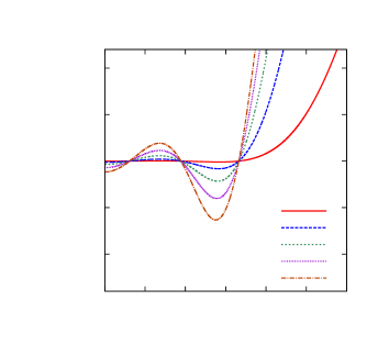
00.050.10.150.20123456

3,maxsubscript3𝑚𝑎𝑥\mathcal{M}_{3,max}

ν𝜈\nufeederRefer to captionN=3𝑁3N=3N=4𝑁4N=4N=5𝑁5N=5N=6𝑁6N=6N=7𝑁7N=7N=14𝑁14N=14
00.20.40.60.810123456ν𝜈\nuhierarchicalRefer to captionN=1𝑁1N=1N=2𝑁2N=2N=3𝑁3N=3N=4𝑁4N=4N=5𝑁5N=5N=12
Figure 12: Left: we plot the maximum value of 3subscript3\mathcal{M}_{3} for which the PDF (for various truncations N𝑁N) produces results within 20%percent2020\% error for ν𝜈\nu specified on the x-axis to νmax=2.1ν0.7subscript𝜈𝑚𝑎𝑥2.1superscript𝜈0.7\nu_{max}=2.1\nu^{0.7} for feeder scaling of higher moments. Right: same as left but for hierarchical scaling and with νmax=2.2ν0.7subscript𝜈𝑚𝑎𝑥2.2superscript𝜈0.7\nu_{max}=2.2\nu^{0.7}.
-0.1-0.0500.050.10123456

error

ν𝜈\nuN=5𝑁5N=5, feederRefer to caption3=0.01subscript30.01\mathcal{M}_{3}=0.013=0.03subscript30.03\mathcal{M}_{3}=0.033=0.05subscript30.05\mathcal{M}_{3}=0.053=0.07subscript30.07\mathcal{M}_{3}=0.073=0.09subscript30.09\mathcal{M}_{3}=0.09
-0.04-0.0200.020.040.060.080.10123456ν𝜈\nuN=3𝑁3N=3, hierarchicalRefer to caption3=0.10subscript30.10\mathcal{M}_{3}=0.103=0.15subscript30.15\mathcal{M}_{3}=0.153=0.20subscript30.20\mathcal{M}_{3}=0.203=0.25subscript30.25\mathcal{M}_{3}=0.253=0.30subscript30.30\mathcal{M}_{3}=0.30
Figure 13: Left: the error of N=5𝑁5N=5 truncation for different values of 3subscript3\mathcal{M}_{3} for feeder scaling. Right: same as left but for hierarchical scaling.

We find that the truncations of the PDF for the feeder scaling generate errors of magnitude >20%absentpercent20>20\% for much smaller ν34𝜈34\nu\approx 3-4 when keeping similar order terms in nsubscript𝑛\mathcal{M}_{n} compared to the hierarchical case (typically ν56𝜈56\nu\approx 5-6 for n=5𝑛5n=5). From Figure 12, we can also see that the value of 3,maxsubscript3𝑚𝑎𝑥\mathcal{M}_{3,max} is much smaller for the feeder scaling and decreases sharply as one increases ν𝜈\nu. This means that at a higher mass range or at higher redshift, our simulation results may not be well described by our analytical formula for the non-Gaussian feeder mass function. Looking at the result for N=14𝑁14N=14, we see that one gains only marginally by increasing the number of terms for the feeder scaling. So, we will adopt N=5𝑁5N=5 truncation for the feeder case (i.e. up to 35/3superscriptsubscript353\mathcal{M}_{3}^{5/3}) to compare with the simulation results. For the hierarchical scaling, we will adopt N=3𝑁3N=3 truncation (i.e up to 35superscriptsubscript35\mathcal{M}_{3}^{5}).

We can also see that the error increases as one increases ν𝜈\nu or 3subscript3\mathcal{M}_{3} (see Figure 13). So, we expect the analytic mass function to describe simulation results better when the level of non-Gaussianity is smaller and at smaller νcsubscript𝜈𝑐\nu_{c} i.e. low redshift and small halo masses.

Also note that our error discussion assumes scalings: nhier=An(3/6)n2superscriptsubscript𝑛hiersubscript𝐴𝑛superscriptsubscript36𝑛2\mathcal{M}_{n}^{\rm hier}=A_{n}(\mathcal{M}_{3}/6)^{n-2} and nfeeder=Bn(3/8)n/3superscriptsubscript𝑛feedersubscript𝐵𝑛superscriptsubscript38𝑛3\mathcal{M}_{n}^{\rm feeder}=B_{n}(\mathcal{M}_{3}/8)^{n/3}. But from our calculated moments, we find that the scaling for the smoothed moments is modified slightly and the higher moments are larger than expected from the simple scaling assumed in the error analysis plots (see Appendix A). The qualitative discussion remains the same but the magnitude of 3,maxsubscript3𝑚𝑎𝑥\mathcal{M}_{3,max} will decrease and the relative error will increase in Figures 12 and 13 respectively.

Appendix C Calculations for bias and stochasticity

Here we calculate the large scale bias and stochasticity expressions for our two field ansatz (2.5). We take as a starting point the derivation for generic non-Gaussian scenarios given in [60]. The leading contribution to the matter-halo cross spectrum, in the long wavelength limit (k0𝑘0k\rightarrow 0) is

Pmh(k)subscript𝑃𝑚𝑘\displaystyle P_{mh}(k) =\displaystyle= bϕ(α2(k)Pϕ,G(k))+α2(k)Pψ,NG(k)[bψ+1α(k)(12(bψ1)δc+12ddlnσR)R(3)]subscript𝑏italic-ϕsuperscript𝛼2𝑘subscript𝑃italic-ϕ𝐺𝑘superscript𝛼2𝑘subscript𝑃𝜓NG𝑘delimited-[]subscript𝑏𝜓1𝛼𝑘12subscript𝑏𝜓1subscript𝛿𝑐12𝑑𝑑subscript𝜎𝑅superscriptsubscript𝑅3\displaystyle b_{\phi}\left(\alpha^{2}(k)P_{\phi,G}(k)\right)+\alpha^{2}(k)P_{\psi,\rm NG}(k)\left[b_{\psi}+\frac{1}{\alpha(k)}\left(\frac{1}{2}(b_{\psi}-1)\delta_{c}+\frac{1}{2}\frac{d}{d\ln\sigma_{R}}\right)\mathcal{F}_{R}^{(3)}\right]
R(3)superscriptsubscript𝑅3\displaystyle\mathcal{F}_{R}^{(3)} =\displaystyle= 1PΦ(k)σR2d3p1(2π)3d3p2(2π)3αR(p1)αR(p2)Φ(k)Φ(p1)Φ(p2)c1subscript𝑃Φ𝑘superscriptsubscript𝜎𝑅2superscript𝑑3subscript𝑝1superscript2𝜋3superscript𝑑3subscript𝑝2superscript2𝜋3subscript𝛼𝑅subscript𝑝1subscript𝛼𝑅subscript𝑝2subscriptdelimited-⟨⟩Φ𝑘Φsubscript𝑝1Φsubscript𝑝2𝑐\displaystyle\frac{1}{P_{\Phi}(k)\sigma_{R}^{2}}\int\frac{d^{3}\vec{p_{1}}}{(2\pi)^{3}}\frac{d^{3}\vec{p_{2}}}{(2\pi)^{3}}\,\alpha_{R}(p_{1})\alpha_{R}(p_{2})\langle\Phi(\vec{k})\Phi(\vec{p_{1}})\Phi(\vec{p_{2}})\rangle_{c}

where αR(k)=WR(k)α(k)subscript𝛼𝑅𝑘subscript𝑊𝑅𝑘𝛼𝑘\alpha_{R}(k)=W_{R}(k)\alpha(k). This expression agrees with the result previously derived in [58]. For our bispectrum, Eq.(2.9), there are two terms in R(3)superscriptsubscript𝑅3\mathcal{F}_{R}^{(3)}. In the k0𝑘0k\rightarrow 0 limit, the usual term (proportional to f~NLsubscript~𝑓NL\tilde{f}_{\rm NL}) is

R,1(3)superscriptsubscript𝑅13\displaystyle\mathcal{F}_{R,1}^{(3)} =\displaystyle= 4f~NLq2[1+f~NL2q𝒫ψ,G(k)I1(k)]1σR2d3p(2π)3αR(p)2PΦ(p)[1+f~NL2q𝒫ψ,G(p)I1(p)]4subscript~𝑓NLsuperscript𝑞2delimited-[]1superscriptsubscript~𝑓NL2𝑞subscript𝒫𝜓𝐺𝑘subscript𝐼1𝑘1superscriptsubscript𝜎𝑅2superscript𝑑3𝑝superscript2𝜋3subscript𝛼𝑅superscript𝑝2subscript𝑃Φ𝑝delimited-[]1superscriptsubscript~𝑓NL2𝑞subscript𝒫𝜓𝐺𝑝subscript𝐼1𝑝\displaystyle\frac{4\tilde{f}_{\rm NL}q^{2}}{[1+\tilde{f}_{\rm NL}^{2}q\mathcal{P}_{\psi,G}(k)I_{1}(k)]}\frac{1}{\sigma_{R}^{2}}\int\frac{d^{3}\vec{p}}{(2\pi)^{3}}\frac{\alpha_{R}(p)^{2}P_{\Phi}(p)}{[1+{\tilde{f}_{\rm NL}^{2}q\mathcal{P}_{\psi,G}(p)I_{1}(p)}]}
\displaystyle\approx 4f~NLq24subscript~𝑓NLsuperscript𝑞2\displaystyle 4\tilde{f}_{\rm NL}q^{2}

where the second line holds only if the non-Gaussian correction to the total power is negligible. In the above expression, we have used,

Pψ,G(k)=qPΦ(k)1+f~NL2q𝒫ψ,GI1(k)subscript𝑃𝜓𝐺𝑘𝑞subscript𝑃Φ𝑘1superscriptsubscript~𝑓NL2𝑞subscript𝒫𝜓𝐺subscript𝐼1𝑘P_{\psi,G}(k)=\frac{q\,P_{\Phi}(k)}{1+\tilde{f}_{\rm NL}^{2}q\mathcal{P}_{\psi,G}I_{1}(k)} (C.3)

which relates the Gaussian power in the ψ,G𝜓𝐺\psi,G field to the total power, PΦsubscript𝑃ΦP_{\Phi}.

The second term, which is usually dropped as small in single field scenarios, is

R,2(3)superscriptsubscript𝑅23\displaystyle\mathcal{F}_{R,2}^{(3)} =\displaystyle= 8f~NL3PΦ(k)σR2d3p1(2π)3αR(p1)αR(|p1+k|)d3p(2π)3Pψ,G(p)Pψ,G(|p1p|)Pψ,G(|p+k|)8superscriptsubscript~𝑓NL3subscript𝑃Φ𝑘superscriptsubscript𝜎𝑅2superscript𝑑3subscript𝑝1superscript2𝜋3subscript𝛼𝑅subscript𝑝1subscript𝛼𝑅subscript𝑝1𝑘superscript𝑑3𝑝superscript2𝜋3subscript𝑃𝜓𝐺𝑝subscript𝑃𝜓𝐺subscript𝑝1𝑝subscript𝑃𝜓𝐺𝑝𝑘\displaystyle\frac{8\tilde{f}_{\rm NL}^{3}}{P_{\Phi}(k)\sigma_{R}^{2}}\int\frac{d^{3}\vec{p_{1}}}{(2\pi)^{3}}\alpha_{R}(p_{1})\alpha_{R}(|\vec{p_{1}}+\vec{k}|)\int\frac{d^{3}\vec{p}}{(2\pi)^{3}}P_{\psi,G}(p)P_{\psi,G}(|\vec{p}_{1}-\vec{p}|)P_{\psi,G}(|\vec{p}+\vec{k}|)

Let us now try to simplify the integral by looking at the major contributions to the integral. At large scales (small k𝑘k), the value of R(3)superscriptsubscript𝑅3\mathcal{F}_{R}^{(3)} peaks when p1subscript𝑝1p_{1} is near the halo scale (1/Rabsent1𝑅\approx 1/R). Typically, when looking at large scale bias, kp1much-less-than𝑘subscript𝑝1k\ll p_{1}. In this squeezed limit, we find that the loop bispectrum can be well approximated by:

d3p(2π)3Pψ,G(p)Pψ,G(|p1p|)Pψ,G(|p+k|)Pψ,G(p1)d3p(2π)3Pψ,G(p)Pψ,G(|p+k|)superscript𝑑3𝑝superscript2𝜋3subscript𝑃𝜓𝐺𝑝subscript𝑃𝜓𝐺subscript𝑝1𝑝subscript𝑃𝜓𝐺𝑝𝑘subscript𝑃𝜓𝐺subscript𝑝1superscript𝑑3𝑝superscript2𝜋3subscript𝑃𝜓𝐺𝑝subscript𝑃𝜓𝐺𝑝𝑘\displaystyle\int\frac{d^{3}\vec{p}}{(2\pi)^{3}}P_{\psi,G}(p)P_{\psi,G}(|\vec{p_{1}}-\vec{p}|)P_{\psi,G}(|\vec{p}+\vec{k}|)\approx P_{\psi,G}(p_{1})\int\frac{d^{3}\vec{p}}{(2\pi)^{3}}P_{\psi,G}(p)P_{\psi,G}(|\vec{p}+\vec{k}|)
(C.4)

This is true because the dominant term for the integral comes from when |p+k|𝑝𝑘|\vec{p}+\vec{k}| and pk𝑝𝑘p\approx k are both small. This approximation breaks down as the ratio p1/ksubscript𝑝1𝑘p_{1}/k becomes smaller. However, we find that the dependence of the left hand side integral on the angular part of p1subscript𝑝1\vec{p_{1}} is symmetric around the approximate value on the right hand side even when p1subscript𝑝1p_{1} is only a few times larger than k𝑘k. Since we integrate over p1subscript𝑝1\vec{p_{1}} in the R(3)superscriptsubscript𝑅3\mathcal{F}_{R}^{(3)} integral, we expect the following approximation to hold quite well.

R,2(3)superscriptsubscript𝑅23\displaystyle\mathcal{F}_{R,2}^{(3)} \displaystyle\approx 8f~NL3PΦ(k)σR2d3p1(2π)3αR(p1)2Pψ,G(p1)d3p(2π)3Pψ,G(p)Pψ,G(|p+k|)8superscriptsubscript~𝑓NL3subscript𝑃Φ𝑘superscriptsubscript𝜎𝑅2superscript𝑑3subscript𝑝1superscript2𝜋3subscript𝛼𝑅superscriptsubscript𝑝12subscript𝑃𝜓𝐺subscript𝑝1superscript𝑑3𝑝superscript2𝜋3subscript𝑃𝜓𝐺𝑝subscript𝑃𝜓𝐺𝑝𝑘\displaystyle\frac{8\tilde{f}_{\rm NL}^{3}}{P_{\Phi}(k)\sigma_{R}^{2}}\int\frac{d^{3}\vec{p_{1}}}{(2\pi)^{3}}\alpha_{R}(p_{1})^{2}P_{\psi,G}(p_{1})\int\frac{d^{3}\vec{p}}{(2\pi)^{3}}P_{\psi,G}(p)P_{\psi,G}(|\vec{p}+\vec{k}|) (C.5)
=\displaystyle= 8f~NL3PΦ(k)σR,ψ2σR2d3p(2π)3Pψ,G(p)Pψ,G(|p+k|)8superscriptsubscript~𝑓NL3subscript𝑃Φ𝑘superscriptsubscript𝜎𝑅𝜓2superscriptsubscript𝜎𝑅2superscript𝑑3𝑝superscript2𝜋3subscript𝑃𝜓𝐺𝑝subscript𝑃𝜓𝐺𝑝𝑘\displaystyle\frac{8\tilde{f}_{\rm NL}^{3}}{P_{\Phi}(k)}\frac{\sigma_{R,\psi}^{2}}{\sigma_{R}^{2}}\int\frac{d^{3}\vec{p}}{(2\pi)^{3}}P_{\psi,G}(p)P_{\psi,G}(|\vec{p}+\vec{k}|)

Approximation (C.5) was checked numerically using the CUBA library for multi-dimensional integration [75]; the result is shown in Figure 14. Further, we also tested that the derivative term in Eq.(LABEL:eq:Pmh) is indeed small compared to relevant values of (bg1)δcR(3)subscript𝑏𝑔1subscript𝛿𝑐superscriptsubscript𝑅3(b_{g}-1)\delta_{c}\mathcal{F}_{R}^{(3)}. The derivative term for feeder scaling ddlnσRR,2(3)𝑑𝑑subscript𝜎𝑅superscriptsubscript𝑅23\frac{d}{d\ln{\sigma_{R}}}\mathcal{F}_{R,2}^{(3)} was found to be of the same order as the derivative term for hierarchical scaling ddlnσRR,1(3)𝑑𝑑subscript𝜎𝑅superscriptsubscript𝑅13\frac{d}{d\ln{\sigma_{R}}}\mathcal{F}_{R,1}^{(3)}.

0.010.11100.01k(hMpc1)𝑘superscriptMpc1k\;(h\;\rm Mpc^{-1})Refer to captionR,2(3)superscriptsubscript𝑅23\mathcal{F}_{R,2}^{(3)}R,2(3)|approxevaluated-atsuperscriptsubscript𝑅23approx\mathcal{F}_{R,2}^{(3)}|_{\rm approx}
Figure 14: Here we test the approximation (C.5) for R,2(3)superscriptsubscript𝑅23\mathcal{F}_{R,2}^{(3)} numerically for R=8Mpc/h𝑅8MpchR=8\;\rm Mpc/h. The approximation is excellent at large scales k0.04hMpc1less-than-or-similar-to𝑘0.04superscriptMpc1k\lesssim 0.04\;h\rm Mpc^{-1}. Note that a different choice for f~NLsubscript~𝑓NL\tilde{f}_{\rm NL} and normalization for Pψ,Gsubscript𝑃𝜓𝐺P_{\psi,G} (or q𝑞q) only rescales both curves by the same factor.

The approximated expression for bias can also be obtained directly from a peak background split analysis of our model. Following the peak background split derivation of [60] (section 4.1.1), as usual, we split both our Gaussian fields into short and long wavelength modes: ϕG(x)=ϕG,l(x)+ϕG,s(x)subscriptitalic-ϕ𝐺𝑥subscriptitalic-ϕ𝐺𝑙𝑥subscriptitalic-ϕ𝐺𝑠𝑥\phi_{G}(\vec{x})=\phi_{G,l}(\vec{x})+\phi_{G,s}(\vec{x}) and ψG(x)=ψG,l(x)+ψG,s(x)subscript𝜓𝐺𝑥subscript𝜓𝐺𝑙𝑥subscript𝜓𝐺𝑠𝑥\psi_{G}(\vec{x})=\psi_{G,l}(\vec{x})+\psi_{G,s}(\vec{x}). However, we also include the ψ(x)2𝜓superscript𝑥2\psi(\vec{x})^{2} term and the local small scale power is given by: σR2=σR2¯[1+4σψ,R2σR2f~NLψl(x)(1+f~NLψl(x)]\sigma_{R}^{2}=\bar{\sigma_{R}^{2}}\left[1+4\frac{\sigma_{\psi,R}^{2}}{\sigma_{R}^{2}}\tilde{f}_{\rm NL}\psi_{l}(\vec{x})\left(1+\tilde{f}_{\rm NL}\psi_{l}(\vec{x}\right)\right]. Then, allowing for separate linear bias coefficients for our two independent fields, we get:

δh(k)subscript𝛿𝑘\displaystyle\delta_{h}(\vec{k}) =\displaystyle= bϕδϕ(k)+bψδψ,NG+2δc(bψ1)f~NLσR,ψ2σR2(ψl(k)+f~NLd3s(2π)3ψl(s)ψl(ks))subscript𝑏italic-ϕsubscript𝛿italic-ϕ𝑘subscript𝑏𝜓subscript𝛿𝜓NG2subscript𝛿𝑐subscript𝑏𝜓1subscript~𝑓NLsuperscriptsubscript𝜎𝑅𝜓2superscriptsubscript𝜎𝑅2subscript𝜓𝑙𝑘subscript~𝑓NLsuperscript𝑑3𝑠superscript2𝜋3subscript𝜓𝑙𝑠subscript𝜓𝑙𝑘𝑠\displaystyle b_{\phi}\delta_{\phi}(\vec{k})+b_{\psi}\delta_{\psi,\rm NG}+2\delta_{c}(b_{\psi}-1)\tilde{f}_{\rm NL}\frac{\sigma_{R,\psi}^{2}}{\sigma_{R}^{2}}\left(\psi_{l}(\vec{k})+\tilde{f}_{\rm NL}\int\frac{d^{3}\vec{s}}{(2\pi)^{3}}\psi_{l}(\vec{s})\psi_{l}(\vec{k}-\vec{s})\right) (C.6)
=\displaystyle= bϕδϕ(k)+(bψ+2δc(bψ1)f~NLα(k)σR,ψ2σR2)δψ,NGsubscript𝑏italic-ϕsubscript𝛿italic-ϕ𝑘subscript𝑏𝜓2subscript𝛿𝑐subscript𝑏𝜓1subscript~𝑓NL𝛼𝑘superscriptsubscript𝜎𝑅𝜓2superscriptsubscript𝜎𝑅2subscript𝛿𝜓NG\displaystyle b_{\phi}\delta_{\phi}(\vec{k})+\left(b_{\psi}+2\delta_{c}(b_{\psi}-1)\frac{\tilde{f}_{\rm NL}}{\alpha(k)}\frac{\sigma_{R,\psi}^{2}}{\sigma_{R}^{2}}\right)\delta_{\psi,\rm NG}

where

δϕ(k)subscript𝛿italic-ϕ𝑘\displaystyle\delta_{\phi}(\vec{k}) =\displaystyle= α(k)ϕl(k)𝛼𝑘subscriptitalic-ϕ𝑙𝑘\displaystyle\alpha(k)\phi_{l}(\vec{k}) (C.7)
δψ,NGsubscript𝛿𝜓NG\displaystyle\delta_{\psi,\rm NG} =\displaystyle= α(k)ψl(k)+f~NLd3p(2π)3α(k)ψl(p)ψl(kp)𝛼𝑘subscript𝜓𝑙𝑘subscript~𝑓NLsuperscript𝑑3𝑝superscript2𝜋3𝛼𝑘subscript𝜓𝑙𝑝subscript𝜓𝑙𝑘𝑝\displaystyle\alpha(k)\psi_{l}(\vec{k})+\tilde{f}_{\rm NL}\int\frac{d^{3}\vec{p}}{(2\pi)^{3}}\alpha(k)\psi_{l}(\vec{p})\psi_{l}(\vec{k}-\vec{p}) (C.8)

and therefore, the total linear matter density field is,

δm(k)subscript𝛿𝑚𝑘\displaystyle\delta_{m}(\vec{k}) =\displaystyle= δϕ(k)+δψ,NGsubscript𝛿italic-ϕ𝑘subscript𝛿𝜓NG\displaystyle\delta_{\phi}(\vec{k})+\delta_{\psi,\rm NG} (C.9)

This gives the expression for Phm(k)subscript𝑃𝑚𝑘P_{hm}(k) to be,

Phm(k)subscript𝑃𝑚𝑘\displaystyle P_{hm}(k) =\displaystyle= bϕα2(k)Pϕ(k)+(bψ+2δc(bψ1)f~NLα(k)σR,ψ2σR2)α2(k)Pψ,NGsubscript𝑏italic-ϕsuperscript𝛼2𝑘subscript𝑃italic-ϕ𝑘subscript𝑏𝜓2subscript𝛿𝑐subscript𝑏𝜓1subscript~𝑓NL𝛼𝑘superscriptsubscript𝜎𝑅𝜓2superscriptsubscript𝜎𝑅2superscript𝛼2𝑘subscript𝑃𝜓NG\displaystyle b_{\phi}\alpha^{2}(k)P_{\phi}(k)+\left(b_{\psi}+2\delta_{c}(b_{\psi}-1)\frac{\tilde{f}_{\rm NL}}{\alpha(k)}\frac{\sigma_{R,\psi}^{2}}{\sigma_{R}^{2}}\right)\alpha^{2}(k)P_{\psi,\rm NG} (C.10)

which agrees to the bias for our two field model given by Eq.(LABEL:eq:Pmh) after using the approximations for R,1(3)superscriptsubscript𝑅13\mathcal{F}_{R,1}^{(3)} and R,2(3)superscriptsubscript𝑅23\mathcal{F}_{R,2}^{(3)} from Eq.(C) and Eq.(C.5). Note that the factor σR,ψ2/σR2qsuperscriptsubscript𝜎𝑅𝜓2superscriptsubscript𝜎𝑅2𝑞\sigma_{R,\psi}^{2}/\sigma_{R}^{2}\approx q for the case of small non-Gaussianity; in this limit one gets the simpler expression Eq.(3.2) but since we do not always stay in the limit of small non-Gaussianity in our simulations, we compute this factor given a model specified by q,f~NL𝑞subscript~𝑓NLq,\tilde{f}_{\rm NL} in our analysis.

Now to compute the stochastic bias, defined as

r2(k)superscript𝑟2𝑘\displaystyle r^{2}(k) =\displaystyle= Phm2(k)Phh(k)Pmm(k)superscriptsubscript𝑃𝑚2𝑘subscript𝑃𝑘subscript𝑃𝑚𝑚𝑘\displaystyle\frac{P_{hm}^{2}(k)}{P_{hh}(k)P_{mm}(k)} (C.11)

we need the halo-halo power spectrum. The leading contributions to the halo-halo power spectrum are

Phh(k)subscript𝑃𝑘\displaystyle P_{hh}(k) =\displaystyle= bϕ2(α2(k)Pϕ,G(k))+α2(k)Pψ,NG(k)[bψ2+2bψα(k)(12(bψ1)δc+12ddlnσR)R(3)\displaystyle b_{\phi}^{2}(\alpha^{2}(k)P_{\phi,G}(k))+\alpha^{2}(k)P_{\psi,NG}(k)\left[b_{\psi}^{2}+\frac{2b_{\psi}}{\alpha(k)}\left(\frac{1}{2}(b_{\psi}-1)\delta_{c}+\frac{1}{2}\frac{d}{d\ln\sigma_{R}}\right)\mathcal{F}_{R}^{(3)}\right. (C.12)
+1α(k)2(12(bψ1)δc+12ddlnσR)2R(4)]\displaystyle\left.+\frac{1}{\alpha(k)^{2}}\left(\frac{1}{2}(b_{\psi}-1)\delta_{c}+\frac{1}{2}\frac{d}{d\ln\sigma_{R}}\right)^{2}\mathcal{F}_{R}^{(4)}\right]
R(4)superscriptsubscript𝑅4\displaystyle\mathcal{F}_{R}^{(4)} =\displaystyle= 1PΦ(k)σR4d3p1(2π)3d3p2(2π)3αR2(p1)αR2(p2)Φ(p1)Φ(kp1)Φ(p2)Φ(kp2)c1subscript𝑃Φ𝑘superscriptsubscript𝜎𝑅4superscript𝑑3subscript𝑝1superscript2𝜋3superscript𝑑3subscript𝑝2superscript2𝜋3superscriptsubscript𝛼𝑅2subscript𝑝1superscriptsubscript𝛼𝑅2subscript𝑝2subscriptdelimited-⟨⟩Φsubscript𝑝1Φ𝑘subscript𝑝1Φsubscript𝑝2Φ𝑘subscript𝑝2𝑐\displaystyle\frac{1}{P_{\Phi}(k)\sigma_{R}^{4}}\int\frac{d^{3}\vec{p_{1}}}{(2\pi)^{3}}\frac{d^{3}\vec{p_{2}}}{(2\pi)^{3}}\,\alpha_{R}^{2}(p_{1})\alpha_{R}^{2}(p_{2})\langle\Phi(\vec{p_{1}})\Phi(\vec{k}-\vec{p}_{1})\Phi(\vec{p_{2}})\Phi(-\vec{k}-\vec{p}_{2})\rangle_{c}

From our trispectrum, Eq.(2.10), there are two terms in R(4)superscriptsubscript𝑅4\mathcal{F}_{R}^{(4)}. In the k0𝑘0k\rightarrow 0 limit, the usual term (proportional to f~NL2superscriptsubscript~𝑓NL2\tilde{f}_{\rm NL}^{2}) is

R,1(4)superscriptsubscript𝑅14\displaystyle\mathcal{F}_{R,1}^{(4)} =\displaystyle= 16f~NL2q3[1+qf~NL2I1(k)𝒫ψ,G(k)][1σR2d3p(2π)3αR(p)2PΦ(p)[1+qf~NL2I1(p)𝒫ψ,G(p)]]216superscriptsubscript~𝑓NL2superscript𝑞3delimited-[]1𝑞superscriptsubscript~𝑓NL2subscript𝐼1𝑘subscript𝒫𝜓𝐺𝑘superscriptdelimited-[]1superscriptsubscript𝜎𝑅2superscript𝑑3𝑝superscript2𝜋3subscript𝛼𝑅superscript𝑝2subscript𝑃Φ𝑝delimited-[]1𝑞superscriptsubscript~𝑓NL2subscript𝐼1𝑝subscript𝒫𝜓𝐺𝑝2\displaystyle\frac{16\tilde{f}_{\rm NL}^{2}q^{3}}{[1+q\tilde{f}_{\rm NL}^{2}I_{1}(k)\mathcal{P}_{\psi,G}(k)]}\left[\frac{1}{\sigma_{R}^{2}}\int\frac{d^{3}p}{(2\pi)^{3}}\frac{\alpha_{R}(p)^{2}P_{\Phi}(p)}{[1+{q\tilde{f}_{\rm NL}^{2}}I_{1}(p)\mathcal{P}_{\psi,G}(p)]}\right]^{2}
\displaystyle\approx 16f~NL2q316superscriptsubscript~𝑓NL2superscript𝑞3\displaystyle 16\tilde{f}_{\rm NL}^{2}q^{3}

The other term, usually much smaller than the first term in single field cases, is

R,2(4)superscriptsubscript𝑅24\displaystyle\mathcal{F}_{R,2}^{(4)} =\displaystyle= 48f~NL4PΦ(k)σR4d3p1(2π)3d3p2(2π)3αR2(p1)αR2(p2)d3p(2π)348superscriptsubscript~𝑓NL4subscript𝑃Φ𝑘superscriptsubscript𝜎𝑅4superscript𝑑3subscript𝑝1superscript2𝜋3superscript𝑑3subscript𝑝2superscript2𝜋3superscriptsubscript𝛼𝑅2subscript𝑝1superscriptsubscript𝛼𝑅2subscript𝑝2superscript𝑑3𝑝superscript2𝜋3\displaystyle\frac{48\tilde{f}_{\rm NL}^{4}}{P_{\Phi}(k)\sigma_{R}^{4}}\int\frac{d^{3}\vec{p_{1}}}{(2\pi)^{3}}\frac{d^{3}\vec{p_{2}}}{(2\pi)^{3}}\alpha_{R}^{2}(p_{1})\alpha_{R}^{2}(p_{2})\int\frac{d^{3}\vec{p}}{(2\pi)^{3}} (C.14)
[Pψ,G(p)Pψ,G(|p1p|)Pψ,G(|kp1+p|)Pψ,G(|pp1p2|)]delimited-[]subscript𝑃𝜓𝐺𝑝subscript𝑃𝜓𝐺subscript𝑝1𝑝subscript𝑃𝜓𝐺𝑘subscript𝑝1𝑝subscript𝑃𝜓𝐺𝑝subscript𝑝1subscript𝑝2\displaystyle\left[P_{\psi,G}(p)P_{\psi,G}(|\vec{p_{1}}-\vec{p}|)P_{\psi,G}(|\vec{k}-\vec{p_{1}}+\vec{p}|)P_{\psi,G}(|\vec{p}-\vec{p_{1}}-\vec{p_{2}}|)\right]

Similar to the case of R,2(3)superscriptsubscript𝑅23\mathcal{F}_{R,2}^{(3)}, we can approximate this integral at large scales by looking at the collapsed limit: kp1,p2much-less-than𝑘subscript𝑝1subscript𝑝2k\ll p_{1},p_{2}. In this limit, the loop trispectrum is well approximated by:

d3p(2π)3Pψ,G(p)Pψ,G(|p1p|)Pψ,G(|kp1+p|)Pψ,G(|pp1p2|)superscript𝑑3𝑝superscript2𝜋3subscript𝑃𝜓𝐺𝑝subscript𝑃𝜓𝐺subscript𝑝1𝑝subscript𝑃𝜓𝐺𝑘subscript𝑝1𝑝subscript𝑃𝜓𝐺𝑝subscript𝑝1subscript𝑝2\displaystyle\int\frac{d^{3}\vec{p}}{(2\pi)^{3}}P_{\psi,G}(p)P_{\psi,G}(|\vec{p_{1}}-\vec{p}|)P_{\psi,G}(|\vec{k}-\vec{p_{1}}+\vec{p}|)P_{\psi,G}(|\vec{p}-\vec{p_{1}}-\vec{p_{2}}|) \displaystyle\approx
Pψ,G(p2)d3p(2π)3Pψ,G(p)Pψ,G(|p1p|)Pψ,G(|p1+k+p|)subscript𝑃𝜓𝐺subscript𝑝2superscript𝑑3𝑝superscript2𝜋3subscript𝑃𝜓𝐺𝑝subscript𝑃𝜓𝐺subscript𝑝1𝑝subscript𝑃𝜓𝐺subscript𝑝1𝑘𝑝\displaystyle P_{\psi,G}(p_{2})\int\frac{d^{3}\vec{p}}{(2\pi)^{3}}P_{\psi,G}(p)P_{\psi,G}(|\vec{p_{1}}-\vec{p}|)P_{\psi,G}(|-\vec{p_{1}}+\vec{k}+\vec{p}|) (C.15)

following from the observation that the integral gets maximum contribution from when |p1p|subscript𝑝1𝑝|\vec{p_{1}}-\vec{p}| is small. Further, when p2/ksubscript𝑝2𝑘p_{2}/k is small, the approximation breaks down as before, but since we integrate over p2subscript𝑝2\vec{p_{2}} to obtain R,2(4)superscriptsubscript𝑅24\mathcal{F}_{R,2}^{(4)}, the symmetry of the integrand with respect to the angular part of p2subscript𝑝2p_{2} will justify the use of this approximation in R,2(4)superscriptsubscript𝑅24\mathcal{F}_{R,2}^{(4)} even when the halo formation scale is only a few times larger than the scale k𝑘k at which stochastic bias is measured.xx

With this approximation R,2(4)superscriptsubscript𝑅24\mathcal{F}_{R,2}^{(4)} becomes,

R,2(4)superscriptsubscript𝑅24\displaystyle\mathcal{F}_{R,2}^{(4)} \displaystyle\approx 48f~NL4σψ,R2PΦ(k)σR4d3p1(2π)3αR2(p1)d3p(2π)3Pψ,G(p)Pψ,G(|p1p|)Pψ,G(|kp1+p|)48superscriptsubscript~𝑓NL4superscriptsubscript𝜎𝜓𝑅2subscript𝑃Φ𝑘superscriptsubscript𝜎𝑅4superscript𝑑3subscript𝑝1superscript2𝜋3superscriptsubscript𝛼𝑅2subscript𝑝1superscript𝑑3𝑝superscript2𝜋3subscript𝑃𝜓𝐺𝑝subscript𝑃𝜓𝐺subscript𝑝1𝑝subscript𝑃𝜓𝐺𝑘subscript𝑝1𝑝\displaystyle\frac{48\tilde{f}_{\rm NL}^{4}\sigma_{\psi,R}^{2}}{P_{\Phi}(k)\sigma_{R}^{4}}\int\frac{d^{3}\vec{p_{1}}}{(2\pi)^{3}}\alpha_{R}^{2}(p_{1})\int\frac{d^{3}\vec{p}}{(2\pi)^{3}}P_{\psi,G}(p)P_{\psi,G}(|\vec{p_{1}}-\vec{p}|)P_{\psi,G}(|\vec{k}-\vec{p_{1}}+\vec{p}|)

These integrals are computationally challenging. However, as in the case of Phm(k)subscript𝑃𝑚𝑘P_{hm}(k), we expect the peak-background-split calculation to provide good approximation, in the large scale limit, to the halo-halo power spectrum. For this, using Eq.(C.6), one obtains,

Phh(k)subscript𝑃𝑘\displaystyle P_{hh}(k) =\displaystyle= bϕ2(α2(k)Pϕ(k))+(bψ+2δc(bψ1)f~NLα(k)σR,ψ2σR2)2α2(k)Pψ,NGsuperscriptsubscript𝑏italic-ϕ2superscript𝛼2𝑘subscript𝑃italic-ϕ𝑘superscriptsubscript𝑏𝜓2subscript𝛿𝑐subscript𝑏𝜓1subscript~𝑓NL𝛼𝑘superscriptsubscript𝜎𝑅𝜓2superscriptsubscript𝜎𝑅22superscript𝛼2𝑘subscript𝑃𝜓NG\displaystyle b_{\phi}^{2}(\alpha^{2}(k)P_{\phi}(k))+\left(b_{\psi}+2\delta_{c}(b_{\psi}-1)\frac{\tilde{f}_{\rm NL}}{\alpha(k)}\frac{\sigma_{R,\psi}^{2}}{\sigma_{R}^{2}}\right)^{2}\alpha^{2}(k)P_{\psi,\rm NG} (C.17)

To summarize this section, we have derived expressions Eq.(C.10) (for Phm(k)subscript𝑃𝑚𝑘P_{hm}(k)) and Eq.(C.17) (for Phh(k)subscript𝑃𝑘P_{hh}(k)), which were used to fit to our simulation results for large scale bias and stochastic bias (Eq.(3.13)).

References

  • [1] Planck Collaboration, P. Ade et al., Planck 2013 Results. XXIV. Constraints on primordial non-Gaussianity, arXiv:1303.5084.
  • [2] A. Pillepich, C. Porciani, and T. H. Reiprich, The X-ray cluster survey with eROSITA: forecasts for cosmology, cluster physics, and primordial non-Gaussianity, Mon.Not.Roy.Astron.Soc. 422 (2012) 44–69, [arXiv:1111.6587].
  • [3] C. Cunha, D. Huterer, and O. Dore, Primordial non-Gaussianity from the covariance of galaxy cluster counts, Phys.Rev. D82 (2010) 023004, [arXiv:1003.2416].
  • [4] M. Oguri, Self-Calibrated Cluster Counts as a Probe of Primordial Non-Gaussianity, Phys.Rev.Lett. 102 (2009) 211301, [arXiv:0905.0920].
  • [5] T. Giannantonio, C. Porciani, J. Carron, A. Amara, and A. Pillepich, Constraining primordial non-Gaussianity with future galaxy surveys, Mon.Not.Roy.Astron.Soc. 422 (2012) 2854–2877, [arXiv:1109.0958].
  • [6] A. Merloni, P. Predehl, W. Becker, H. Bohringer, T. Boller, et al., eROSITA Science Book: Mapping the Structure of the Energetic Universe, arXiv:1209.3114.
  • [7] Euclid Theory Working Group Collaboration, L. Amendola et al., Cosmology and fundamental physics with the Euclid satellite, Living Rev.Rel. 16 (2013) 6, [arXiv:1206.1225].
  • [8] D. Jeong and E. Komatsu, Primordial non-Gaussianity, scale-dependent bias, and the bispectrum of galaxies, Astrophys.J. 703 (2009) 1230–1248, [arXiv:0904.0497].
  • [9] T. Baldauf, U. Seljak, and L. Senatore, Primordial non-Gaussianity in the Bispectrum of the Halo Density Field, JCAP 1104 (2011) 006, [arXiv:1011.1513].
  • [10] G. Tasinato, M. Tellarini, A. J. Ross, and D. Wands, Primordial non-Gaussianity in the bispectra of large-scale structure, arXiv:1310.7482.
  • [11] N. Barnaby and S. Shandera, Feeding your Inflaton: Non-Gaussian Signatures of Interaction Structure, JCAP 1201 (2012) 034, [arXiv:1109.2985].
  • [12] M. LoVerde, A. Miller, S. Shandera, and L. Verde, Effects of Scale-Dependent Non-Gaussianity on Cosmological Structures, JCAP 0804 (2008) 014, [arXiv:0711.4126].
  • [13] S. Shandera, A. Mantz, D. Rapetti, and S. W. Allen, X-ray Cluster Constraints on Non-Gaussianity, JCAP 1308 (2013) 004, [arXiv:1304.1216].
  • [14] J. Truemper, ROSAT - A new look at the X-ray sky, Science 260 (June, 1993) 1769–1771.
  • [15] B. Benson, T. de Haan, J. Dudley, C. Reichardt, K. Aird, et al., Cosmological Constraints from Sunyaev-Zel’dovich-Selected Clusters with X-ray Observations in the First 178 Square Degrees of the South Pole Telescope Survey, Astrophys.J. 763 (2013) 147, [arXiv:1112.5435].
  • [16] R. Williamson, B. Benson, F. High, K. Vanderlinde, P. Ade, et al., An SZ-selected sample of the most massive galaxy clusters in the 2500-square-degree South Pole Telescope survey, Astrophys.J. 738 (2011) 139, [arXiv:1101.1290].
  • [17] A. Mana, T. Giannantonio, J. Weller, B. Hoyle, G. Huetsi, et al., Combining clustering and abundances of galaxy clusters to test cosmology and primordial non-Gaussianity, arXiv:1303.0287.
  • [18] N. Afshordi and A. J. Tolley, Primordial non-gaussianity, statistics of collapsed objects, and the Integrated Sachs-Wolfe effect, Phys.Rev. D78 (2008) 123507, [arXiv:0806.1046].
  • [19] A. Slosar, C. Hirata, U. Seljak, S. Ho, and N. Padmanabhan, Constraints on local primordial non-Gaussianity from large scale structure, JCAP 0808 (2008) 031, [arXiv:0805.3580].
  • [20] J.-Q. Xia, A. Bonaldi, C. Baccigalupi, G. De Zotti, S. Matarrese, et al., Constraining Primordial Non-Gaussianity with High-Redshift Probes, JCAP 1008 (2010) 013, [arXiv:1007.1969].
  • [21] J.-Q. Xia, C. Baccigalupi, S. Matarrese, L. Verde, and M. Viel, Constraints on Primordial Non-Gaussianity from Large Scale Structure Probes, JCAP 1108 (2011) 033, [arXiv:1104.5015].
  • [22] A. J. Ross, W. J. Percival, A. Carnero, G.-b. Zhao, M. Manera, et al., The Clustering of Galaxies in SDSS-III DR9 Baryon Oscillation Spectroscopic Survey: Constraints on Primordial Non-Gaussianity, Mon.Not.Roy.Astron.Soc. 428 (2013) 1116–1127, [arXiv:1208.1491].
  • [23] D. Karagiannis, T. Shanks, and N. P. Ross, Search for primordial non-Gaussianity in the quasars of SDSS-III BOSS DR9, arXiv:1310.6716.
  • [24] T. Giannantonio, A. J. Ross, W. J. Percival, R. Crittenden, D. Bacher, et al., Improved Primordial Non-Gaussianity Constraints from Measurements of Galaxy Clustering and the Integrated Sachs-Wolfe Effect, arXiv:1303.1349.
  • [25] S. Ho, N. Agarwal, A. D. Myers, R. Lyons, A. Disbrow, et al., Sloan Digital Sky Survey III Photometric Quasar Clustering: Probing the Initial Conditions of the Universe using the Largest Volume, arXiv:1311.2597.
  • [26] N. Agarwal, S. Ho, and S. Shandera, Constraining the initial conditions of the Universe using large scale structure, arXiv:1311.2606.
  • [27] A. Pillepich, C. Porciani, and O. Hahn, Universal halo mass function and scale-dependent bias from N-body simulations with non-Gaussian initial conditions, arXiv:0811.4176.
  • [28] M. Grossi, L. Verde, C. Carbone, K. Dolag, E. Branchini, et al., Large-scale non-Gaussian mass function and halo bias: tests on N-body simulations, Mon.Not.Roy.Astron.Soc. 398 (2009) 321–332, [arXiv:0902.2013].
  • [29] T. Giannantonio and C. Porciani, Structure formation from non-Gaussian initial conditions: multivariate biasing, statistics, and comparison with N-body simulations, Phys.Rev. D81 (2010) 063530, [arXiv:0911.0017].
  • [30] M. LoVerde and K. M. Smith, The Non-Gaussian Halo Mass Function with fNLsubscript𝑓𝑁𝐿f_{NL}, gNLsubscript𝑔𝑁𝐿g_{NL} and τNLsubscript𝜏𝑁𝐿\tau_{NL}, JCAP 1108 (2011) 003, [arXiv:1102.1439].
  • [31] G. D’Amico, M. Musso, J. Norena, and A. Paranjape, An Improved Calculation of the Non-Gaussian Halo Mass Function, JCAP 1102 (2011) 001, [arXiv:1005.1203].
  • [32] C. Wagner, L. Verde, and L. Boubekeur, N-body simulations with generic non-Gaussian initial conditions I: Power Spectrum and halo mass function, JCAP 1010 (2010) 022, [arXiv:1006.5793].
  • [33] N. Dalal, O. Dore, D. Huterer, and A. Shirokov, The imprints of primordial non-gaussianities on large-scale structure: scale dependent bias and abundance of virialized objects, Phys.Rev. D77 (2008) 123514, [arXiv:0710.4560].
  • [34] D. Tseliakhovich, C. Hirata, and A. Slosar, Non-Gaussianity and large-scale structure in a two-field inflationary model, Phys.Rev. D82 (2010) 043531, [arXiv:1004.3302].
  • [35] A. D. Linde and V. F. Mukhanov, Nongaussian isocurvature perturbations from inflation, Phys.Rev. D56 (1997) 535–539, [astro-ph/9610219].
  • [36] T. Moroi and T. Takahashi, Effects of cosmological moduli fields on cosmic microwave background, Phys.Lett. B522 (2001) 215–221, [hep-ph/0110096].
  • [37] D. H. Lyth and D. Wands, Generating the curvature perturbation without an inflaton, Phys.Lett. B524 (2002) 5–14, [hep-ph/0110002].
  • [38] K. Enqvist and M. S. Sloth, Adiabatic CMB perturbations in pre - big bang string cosmology, Nucl.Phys. B626 (2002) 395–409, [hep-ph/0109214].
  • [39] G. Dvali, A. Gruzinov, and M. Zaldarriaga, A new mechanism for generating density perturbations from inflation, Phys.Rev. D69 (2004) 023505, [astro-ph/0303591].
  • [40] M. Zaldarriaga, Non-Gaussianities in models with a varying inflaton decay rate, Phys.Rev. D69 (2004) 043508, [astro-ph/0306006].
  • [41] P. Creminelli and M. Zaldarriaga, Single field consistency relation for the 3-point function, JCAP 0410 (2004) 006, [astro-ph/0407059].
  • [42] E. Pajer, F. Schmidt, and M. Zaldarriaga, The Observed Squeezed Limit of Cosmological Three-Point Functions, Phys.Rev. D88 (2013), no. 8 083502, [arXiv:1305.0824].
  • [43] R. Keisler, C. Reichardt, K. Aird, B. Benson, L. Bleem, et al., A Measurement of the Damping Tail of the Cosmic Microwave Background Power Spectrum with the South Pole Telescope, Astrophys.J. 743 (2011) 28, [arXiv:1105.3182].
  • [44] Atacama Cosmology Telescope Collaboration, J. L. Sievers et al., The Atacama Cosmology Telescope: Cosmological parameters from three seasons of data, JCAP 1310 (2013) 060, [arXiv:1301.0824].
  • [45] Planck Collaboration, P. Ade et al., Planck 2013 results. XVI. Cosmological parameters, arXiv:1303.5076.
  • [46] D. H. Lyth, Non-gaussianity and cosmic uncertainty in curvaton-type models, JCAP 0606 (2006) 015, [astro-ph/0602285].
  • [47] D. H. Lyth, The curvature perturbation in a box, JCAP 0712 (2007) 016, [arXiv:0707.0361].
  • [48] X. Chen and Y. Wang, Quasi-Single Field Inflation and Non-Gaussianities, JCAP 1004 (2010) 027, [arXiv:0911.3380].
  • [49] E. Nelson and S. Shandera, Statistical Naturalness and non-Gaussianity in a Finite Universe, Phys.Rev.Lett. 110 (2013), no. 13 131301, [arXiv:1212.4550].
  • [50] M. LoVerde, E. Nelson, and S. Shandera, Non-Gaussian Mode Coupling and the Statistical Cosmological Principle, JCAP 1306 (2013) 024, [arXiv:1303.3549].
  • [51] W. H. Press and P. Schechter, Formation of galaxies and clusters of galaxies by selfsimilar gravitational condensation, Astrophys.J. 187 (1974) 425–438.
  • [52] J. L. Tinker, A. V. Kravtsov, A. Klypin, K. Abazajian, M. S. Warren, et al., Toward a halo mass function for precision cosmology: The Limits of universality, Astrophys.J. 688 (2008) 709–728, [arXiv:0803.2706].
  • [53] V. V. Petrov, Sums of independent random variables. Springer-Verlag, 1975.
  • [54] S. Blinnikov and R. Moessner, Expansions for nearly Gaussian distributions, Astron.Astrophys.Suppl.Ser. 130 (1998) 193–205, [astro-ph/9711239].
  • [55] F. Bernardeau, S. Colombi, E. Gaztanaga, and R. Scoccimarro, Large-scale structure of the universe and cosmological perturbation theory, Phys. Rept. 367 (2002) 1–248, [astro-ph/0112551].
  • [56] S. Matarrese, F. Lucchin, and S. A. Bonometto, A Path Integral Approach To Large Scale Matter Distribution Originated By Nongaussian Fluctuations, Astrophys.J. 310 (1986) L21–L26.
  • [57] S. Matarrese and L. Verde, The effect of primordial non-Gaussianity on halo bias, Astrophys.J. 677 (2008) L77–L80, [arXiv:0801.4826].
  • [58] V. Desjacques, D. Jeong, and F. Schmidt, Accurate Predictions for the Scale-Dependent Galaxy Bias from Primordial Non-Gaussianity, Phys.Rev. D84 (2011) 061301, [arXiv:1105.3476].
  • [59] V. Desjacques, D. Jeong, and F. Schmidt, Non-Gaussian Halo Bias Re-examined: Mass-dependent Amplitude from the Peak-Background Split and Thresholding, Phys.Rev. D84 (2011) 063512, [arXiv:1105.3628].
  • [60] D. Baumann, S. Ferraro, D. Green, and K. M. Smith, Stochastic Bias from Non-Gaussian Initial Conditions, JCAP 1305 (2013) 001, [arXiv:1209.2173].
  • [61] S. Yokoyama, Scale-dependent bias from the primordial non-Gaussianity with a Gaussian-squared field, JCAP 1111 (2011) 001, [arXiv:1108.5569].
  • [62] K. M. Smith and M. LoVerde, Local stochastic non-Gaussianity and N-body simulations, JCAP 1111 (2011) 009, [arXiv:1010.0055].
  • [63] V. Springel, The Cosmological simulation code GADGET-2, Mon.Not.Roy.Astron.Soc. 364 (2005) 1105–1134, [astro-ph/0505010].
  • [64] M. Crocce, S. Pueblas, and R. Scoccimarro, Transients from Initial Conditions in Cosmological Simulations, Mon.Not.Roy.Astron.Soc. 373 (2006) 369–381, [astro-ph/0606505].
  • [65] S. R. Knollmann and A. Knebe, Ahf: Amiga’s Halo Finder, Astrophys.J.Suppl. 182 (2009) 608–624, [arXiv:0904.3662].
  • [66] M. Maggiore and A. Riotto, The Halo mass function from excursion set theory. III. Non-Gaussian fluctuations, Astrophys.J. 717 (2010) 526–541, [arXiv:0903.1251].
  • [67] M. Maggiore and A. Riotto, The Halo Mass Function from Excursion Set Theory with a Non-Gaussian Trispectrum, Mon.Not.Roy.Astron.Soc.Lett. 405 (2010) 1244–1252, [arXiv:0910.5125].
  • [68] A. De Simone, M. Maggiore, and A. Riotto, Excursion Set Theory for generic moving barriers and non-Gaussian initial conditions, Mon.Not.Roy.Astron.Soc. 412 (2011) 2587, [arXiv:1007.1903].
  • [69] A. De Simone, M. Maggiore, and A. Riotto, Conditional Probabilities in the Excursion Set Theory. Generic Barriers and non-Gaussian Initial Conditions, Mon.Not.Roy.Astron.Soc. 418 (2011) 2403, [arXiv:1102.0046].
  • [70] M. Musso and R. K. Sheth, The excursion set approach in non-Gaussian random fields, arXiv:1305.0724.
  • [71] I. Achitouv, C. Wagner, J. Weller, and Y. Rasera, Computation of the Halo Mass Function Using Physical Collapse Parameters: Application to Non-Standard Cosmologies, arXiv:1312.1364.
  • [72] T. Baldauf, U. Seljak, R. E. Smith, N. Hamaus, and V. Desjacques, Halo stochasticity from exclusion and nonlinear clustering, Phys.Rev. D88 (2013), no. 8 083507, [arXiv:1305.2917].
  • [73] V. Desjacques, U. Seljak, and I. Iliev, Scale-dependent bias induced by local non-Gaussianity: A comparison to N-body simulations, Mon.Not.Roy.Astron.Soc. 396 (2009) 85–96, [arXiv:0811.2748].
  • [74] S. Shandera, A. L. Erickcek, P. Scott, and J. Y. Galarza, Number Counts and Non-Gaussianity, Phys.Rev. D88 (2013), no. 10 103506, [arXiv:1211.7361].
  • [75] T. Hahn, CUBA: A Library for multidimensional numerical integration, Comput.Phys.Commun. 168 (2005) 78–95, [hep-ph/0404043].