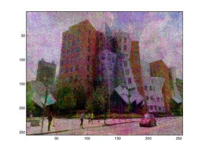
Robust Phase Retrieval and Super-Resolution from One Bit Coded Diffraction Patterns.

Youssef Mroueh,{}^{\dagger},\star
\dagger CBCL, McGovern Institute,& CSAIL, MIT, USA.
\star LCSL, Massachussetts Institute of Technology and Istituto Italiano di Tecnologia.

ymroueh@mit.edu
Abstract

In this paper we study a realistic setup for phase retrieval, where the signal of interest is modulated or masked and then for each modulation or mask a diffraction pattern is collected, producing a coded diffraction pattern (CDP) [CLM13]. We are interested in the setup where the resolution of the collected CDP is limited by the Fraunhofer diffraction limit of the imaging system. We investigate a novel approach based on a geometric quantization scheme of phase-less linear measurements into (one-bit) coded diffraction patterns, and a corresponding recovery scheme. The key novelty in this approach consists in comparing pairs of coded diffractions patterns across frequencies: the one bit measurements obtained rely on the order statistics of the un-quantized measurements rather than their values . This results in a robust phase recovery, and unlike currently available methods, allows to efficiently perform phase recovery from measurements affected by severe (possibly unknown) non linear, rank preserving perturbations, such as distortions. Another important feature of this approach consists in the fact that it enables also super-resolution and blind-deconvolution, beyond the diffraction limit of a given imaging system.

1 Introduction

1.1 The Phase Retrieval Problem and the Diffraction Limit

The problem of phase retrieval is ubiquitous in many areas of imaging science and engineering, where we are able to measure only magnitude of measurements. The phase recovery problem can be modeled as the problem of reconstructing a n𝑛n-dimensional complex vector x0subscript𝑥0x_{0} given only the magnitude of m𝑚m phase-less linear measurements. Such a problem arises for example in X-ray crystallography [Har93, Lea08], diffraction imaging [BDP+07, Rod08] or microscopy [MISE08], where one can only measure the intensities of the incoming waves, and wishes to recover the lost phase in order to be able to reconstruct the desired object. Formally speaking for a given vector x0nsubscript𝑥0superscript𝑛x_{0}\in\mathbb{C}^{n} (without loss of generality we assume n𝑛n to be even), we wish to measure ak,xsubscript𝑎𝑘𝑥\left\langle{a_{k}},{x}\right\rangle, but the only available information is of the form:

bk=θ(|ak,x|2),k=1m,formulae-sequencesubscript𝑏𝑘𝜃superscriptsubscript𝑎𝑘𝑥2𝑘1𝑚b_{k}=\theta(|\left\langle{a_{k}},{x}\right\rangle|^{2}),k=1\dots m, (1)

where aksubscript𝑎𝑘a_{k} is a set of sampling vector in nsuperscript𝑛\mathbb{C}^{n}, and θ𝜃\theta models possibly unknown non linear perturbations of the values: distortion and exponential noise for instance.

Recovering signals from the modulus of their Fourier transform is at the core of the phase retrieval problem. For instance in coherent X-ray crystallography [Lea08], speckle imaging in astronomy [Fri66], in microscopy [Gus00] or more broadly in Fourier optics it follows from the Fraunhofer diffraction principle that the optical field at the detector can be approximated by the Fourier transform of the sensed object. Since light detectors can measure only intensities of the incoming waves the problem is therefore to recover the discrete signal x0nsubscript𝑥0superscript𝑛x_{0}\in\mathbb{C}^{n} from measurements of the type:

bk=θ(|j=1nx0[j]ei2π(j1)(k1)n|2),kΩ,Ω[1,n]formulae-sequencesubscript𝑏𝑘𝜃superscriptsuperscriptsubscript𝑗1𝑛subscript𝑥0delimited-[]𝑗superscript𝑒𝑖2𝜋𝑗1𝑘1𝑛2formulae-sequence𝑘ΩΩ1𝑛b_{k}=\theta\left(\left|\sum_{j=1}^{n}x_{0}[j]e^{-i{2\pi(j-1)\frac{(k-1)}{n}}}\right|^{2}\right),\quad k\in\Omega,\quad\Omega\subseteq[1,n] (2)

where ΩΩ\Omega represents a set of sampled frequencies, and θ𝜃\theta a possibly unknown non-linearity. When compared to (1) we note that in (2) aksubscript𝑎𝑘a_{k} correspond to a set of sampled complex sinusoids. When Ω=[1,n]Ω1𝑛\Omega=[1,n], we have the full knowledge of the modulus of the Fourier series decomposition of the signal of interest on whole ranges of frequencies. In practice due to the Fraunhofer diffraction limit we are able to measure intensities of the Fourier transform within a range of frequencies below the so called cut-off frequency fcsubscript𝑓𝑐f_{c}. Hence the information we have available about x0subscript𝑥0x_{0} is a sample of the lower end of its power spectra in the form of the lowest 2fc+12subscript𝑓𝑐12f_{c}+1 modulus of the Fourier series coefficients (fcsubscript𝑓𝑐f_{c} is an integer).
For instance in microscopy imaging with coherent illumination the object of interest is diffracted through a lens. The lens is characterized by its Point Spread Function (PSF) hh, and the cut-off frequency fc=2πNAνsubscript𝑓𝑐2𝜋𝑁𝐴𝜈f_{c}=\frac{2\pi NA}{\nu}, where NA𝑁𝐴NA is the numerical aperture of the lens and ν𝜈\nu is the wavelength of the illumination light. Let h^,x^0^subscript^𝑥0\hat{h},\hat{x}_{0} be the Fourier transform of the PSF and the signal x0subscript𝑥0x_{0} respectively, for continuous signals we know that:

h^(w)=0 for |w|>fc.formulae-sequence^𝑤0 for 𝑤subscript𝑓𝑐\hat{h}(w)=0\quad\text{ for }|w|>f_{c}.

Hence we measure the modulus of the Fourier transform of x0hsubscript𝑥0x_{0}\star h rather than x0subscript𝑥0x_{0}, where \star denotes the discrete convolution operation. If we set θ=θh𝜃subscript𝜃\theta=\theta_{h}, where

θh(|j=1nx0[j]ei2π(j1)(k1)n|2):=|j=1n(x0h)[j]ei2π(j1)(k1)n|2,assignsubscript𝜃superscriptsuperscriptsubscript𝑗1𝑛subscript𝑥0delimited-[]𝑗superscript𝑒𝑖2𝜋𝑗1𝑘1𝑛2superscriptsuperscriptsubscript𝑗1𝑛subscript𝑥0delimited-[]𝑗superscript𝑒𝑖2𝜋𝑗1𝑘1𝑛2\theta_{h}\left(\left|\sum_{j=1}^{n}x_{0}[j]e^{-i{2\pi(j-1)\frac{(k-1)}{n}}}\right|^{2}\right):=\left|\sum_{j=1}^{n}(x_{0}\star h)[j]e^{-i{2\pi(j-1)\frac{(k-1)}{n}}}\right|^{2},

equation (2) becomes (with some abuse of notation, in re-indexing k𝑘k between n2𝑛2-\frac{n}{2} and n21𝑛21\frac{n}{2}-1 ):

bk=|h^|k2|x^0|k2kfc,fc and bk=0 elsewhere.formulae-sequencesubscript𝑏𝑘subscriptsuperscript^2𝑘subscriptsuperscriptsubscript^𝑥02𝑘𝑘subscript𝑓𝑐subscript𝑓𝑐 and subscript𝑏𝑘0 elsewhereb_{k}=|\hat{h}|^{2}_{k}|\hat{x}_{0}|^{2}_{k}\quad k\in\llbracket-f_{c},f_{c}\rrbracket\text{ and }b_{k}=0\text{ elsewhere}. (3)

It follows from equation (3), that in addition to the missing phase problem we are facing a super-resolution problem since the high frequency content of the signal is also lost due to the physical resolution limit induced by the cut-off frequency fcsubscript𝑓𝑐f_{c} (See for e.g. [Gus00]).
This paper answers the following questions:

  1. 1.

    Robust recovery: Is it possible to robustly recover the missing phase from the power spectra of a signal x0subscript𝑥0x_{0} that is undergoing severe unknown non linear distortions or a stochastic noise?

  2. 2.

    Phase Recovery , Super-Resolution, and Blind deconvolution: Is it possible to recover the signal from the lower end of its power spectra? In other words is it possible to super-resolve the signal beyond the diffraction limit of a given optical system even if the PSF of that system was unknown (blind deconvolution)?

Notations: \star represents a convolution, and direct-product\odot the Hadamard product (component-wise product). For z𝑧z\in\mathbb{C}, |z|2superscript𝑧2|z|^{2} is squared complex modulus of z𝑧z. For a,an𝑎superscript𝑎superscript𝑛a,a^{\prime}\in\mathbb{C}^{n}, a,a𝑎superscript𝑎\left\langle{a},{a^{\prime}}\right\rangle is the complex dot product in nsuperscript𝑛\mathbb{C}^{n}. For an,a𝑎superscript𝑛superscript𝑎a\in\mathbb{C}^{n},a^{*} is the complex conjugate of a, a2subscriptnorm𝑎2||a||_{2} is the norm 222 of a𝑎a and . Let A𝐴A a complex hermitian matrix in nsuperscript𝑛\mathbb{C}^{n}, AFsubscriptnorm𝐴𝐹||A||_{F} denotes the Frobenius norm of A𝐴A, Anorm𝐴||A|| demotes the operator norm of A𝐴A, Tr(A)𝑇𝑟𝐴Tr(A) denotes the trace of A. Throughout the paper, we denote by c,C𝑐𝐶c,C positive absolute constants whose values may change from instance to instance.

1.2 Phase Retrieval: Previous Work

As mentioned in the introduction the set of sampling vectors we are interested in, is the set of complex sinusoids. Before tackling the Fourier based sampling we turn to the setting pioneered by [CSV11] where the set of sampling vectors is randomized, i.e we consider a set of independent measurements defined by independent and identically distributed Complex Gaussian sensing vectors,

ain,ai𝒩(0,12In)+i𝒩(0,12In),i=1m.formulae-sequencesubscript𝑎𝑖superscript𝑛formulae-sequencesimilar-tosubscript𝑎𝑖𝒩012subscript𝐼𝑛𝑖𝒩012subscript𝐼𝑛𝑖1𝑚a_{i}\in\mathbb{C}^{n},\quad\quad a_{i}\sim\mathcal{N}(0,\frac{1}{2}I_{n})+i\mathcal{N}(0,\frac{1}{2}I_{n}),\quad i=1\dots m. (4)

The (noiseless) phase recovery problem is defined as follow.

Definition 1 (Phase-less Sensing and Phase Recovery).

Suppose phase-less sensing measurements

bi=|ai,x0|2+,i=1m,formulae-sequencesubscript𝑏𝑖superscriptsubscript𝑎𝑖subscript𝑥02subscript𝑖1𝑚b_{i}=|\left\langle{a_{i}},{x_{0}}\right\rangle|^{2}\in\mathbb{R}_{+},\quad\quad i=1\dots m, (5)

are given for x0nsubscript𝑥0superscript𝑛x_{0}\in\mathbb{C}^{n}, where ai,i=1,,mformulae-sequencesubscript𝑎𝑖𝑖1𝑚a_{i},~{}i=1,\dots,m are random vectors as in (4). The phase recovery problem is

findx,absentfind𝑥\displaystyle\underset{}{\text{find}~{}x},\quad subject to|ai,x|2=bi,i=1m.formulae-sequencesubject tosuperscriptsubscript𝑎𝑖𝑥2subscript𝑏𝑖𝑖1𝑚\displaystyle\text{subject to}\quad|\left\langle{a_{i}},{x}\right\rangle|^{2}=b_{i},\quad i=1\dots m. (6)

The above problem is non convex and in the following we recall recent approaches to provably and efficiently recover x0subscript𝑥0x_{0} from a finite number of measurements.

SDP (Convex) Relaxation and PhaseLift. The PhaseLift approach [CSV11] stems from the observation that |ai,x|2=Tr(aiaixx),superscriptsubscript𝑎𝑖𝑥2𝑇𝑟subscript𝑎𝑖subscriptsuperscript𝑎𝑖𝑥superscript𝑥|\left\langle{a_{i}},{x}\right\rangle|^{2}=Tr(a_{i}a^{*}_{i}xx^{*}), so that if we let X=xx𝑋𝑥superscript𝑥X=xx^{*}, Problem 6 can be written as,

findX,\displaystyle\underset{}{\text{find}~{}X,} subject to Tr(aiaiX)=bi,i=1m,formulae-sequence𝑇𝑟subscript𝑎𝑖superscriptsubscript𝑎𝑖𝑋subscript𝑏𝑖𝑖1𝑚\displaystyle Tr(a_{i}a_{i}^{*}X)=b_{i},\quad i=1\dots m, X0,rank(X)=1.formulae-sequencesucceeds-or-equals𝑋0𝑟𝑎𝑛𝑘𝑋1\displaystyle\quad X\succeq 0,\quad rank(X)=1. (7)

While the above formulation is still non convex (and in fact combinatorially hard because of the rank constraint), a convex relaxation can be obtained noting that Problem LABEL:PLift can be written as a rank minimization problem over the positive semi-definite cone,

min𝑋rank(X),subject toTr(aiaiX)=bi,i=1m,X0,formulae-sequence𝑋min𝑟𝑎𝑛𝑘𝑋subject to𝑇𝑟subscript𝑎𝑖superscriptsubscript𝑎𝑖𝑋subscript𝑏𝑖formulae-sequence𝑖1𝑚succeeds-or-equals𝑋0\underset{X}{\text{min}}\quad rank(X),\quad\text{subject to}\quad Tr(a_{i}a_{i}^{*}X)=b_{i},~{}~{}i=1\dots m,\quad X\succeq 0, (8)

and then considering the trace as a surrogate for the rank [CSV11],

min𝑋Tr(X),subject toTr(aiaiX)=bi,i=1m,X0.formulae-sequence𝑋min𝑇𝑟𝑋subject to𝑇𝑟subscript𝑎𝑖superscriptsubscript𝑎𝑖𝑋subscript𝑏𝑖formulae-sequence𝑖1𝑚succeeds-or-equals𝑋0\underset{X}{\text{min}}\quad Tr(X),\quad\text{subject to}\quad Tr(a_{i}a_{i}^{*}X)=b_{i},~{}~{}i=1\dots m,\quad X\succeq 0. (9)

Indeed, the above problem is convex and can be solved via semidefinite programming (SDP). Intestingly, a different relaxation is obtained in [DH12] by ignoring the rank constraint in Problem LABEL:PLift. The results in [CSV11, DH12] show that, with high probability, the solution X^msubscript^𝑋𝑚\hat{X}_{m} obtained via either one of the above relaxations can recover x0subscript𝑥0x_{0} exactly i.e. X^m=x0x0subscript^𝑋𝑚subscript𝑥0superscriptsubscript𝑥0\hat{X}_{m}=x_{0}x_{0}^{*}, as soon as mcnlogn𝑚𝑐𝑛𝑛m\geq cn\log n. In fact, the latter requirement can be further improved to mcn𝑚𝑐𝑛m\geq cn [CL12]. While powerful, the convex relaxation approach incur in cumbersome computations, and in practice non convex approaches based on greedy alternating minimization (AM) [GS72, Fie82, GL84] are often used. The convergence properties of the latter methods depend heavily on the initialization and only recently [NJS13] they have been shown to globally converge (with high probability) if provided with a suitable initialization.

Phase Retrieval via Suitably Initialized Alternating Minimization. Let A𝐴A be the matrix defined by m𝑚m sensing vectors as in (4) and B=Diag(b)𝐵𝐷𝑖𝑎𝑔𝑏B=Diag(\sqrt{b}), where b𝑏b is the vector of measurements as in (5). Then

Ax0=Bu0𝐴subscript𝑥0𝐵subscript𝑢0Ax_{0}=Bu_{0}

for u0=Ph(Ax0)subscript𝑢0𝑃𝐴subscript𝑥0u_{0}=Ph(Ax_{0}) with Ph(z)=(z1|z1|,zm|zm|)𝑃𝑧subscript𝑧1subscript𝑧1subscript𝑧𝑚subscript𝑧𝑚Ph(z)=\left(\frac{z_{1}}{|z_{1}|},\dots\frac{z_{m}}{|z_{m}|}\right), zm𝑧superscript𝑚z\in\mathbb{C}^{m}. The above equality suggests the following natural approach to recover (x0,u0)subscript𝑥0subscript𝑢0(x_{0},u_{0}),

minx,uAxBu2,subject to|ui|=1,i=1m,formulae-sequence𝑥𝑢minsuperscriptnorm𝐴𝑥𝐵𝑢2subject tosubscript𝑢𝑖1𝑖1𝑚\underset{x,u}{\text{min}}||Ax-Bu||^{2},\quad\text{subject to}\quad|u_{i}|=1,\quad i=1\dots m,\\ (10)

The above problem is not convex because of the constraint on u𝑢u and the AM approach consists in optimizing u𝑢u, for a given x𝑥x, and then optimizing x𝑥x for a given u𝑢u. It is easy to see that for a given x𝑥x, the optimal u𝑢u is simply u=Ph(Ax),𝑢𝑃𝐴𝑥u=Ph\left(Ax\right), and, for a given u𝑢u, the optimal x𝑥x is the solution of a least square problem. The key result in [NJS13] shows that if such an iteration is initialized with the maximum eigenvector of the matrix

C^m=1mi=1mbiaiaisubscript^𝐶𝑚1𝑚superscriptsubscript𝑖1𝑚subscript𝑏𝑖subscript𝑎𝑖superscriptsubscript𝑎𝑖\hat{C}_{m}=\frac{1}{m}\sum_{i=1}^{m}b_{i}a_{i}a_{i}^{*} (11)

then the solution of the alternating minimization xt0subscript𝑥subscript𝑡0x_{t_{0}} globally converges (with high probability) to the true vector x0subscript𝑥0x_{0}. Throughout this paper we call this initialization SubExp initialization. Moreover for a given accuracy ϵ,0<ϵ<1italic-ϵ0italic-ϵ1\epsilon,0<\epsilon<1, if

mc(n(log3n+log1ϵloglog1ϵ)),𝑚𝑐𝑛superscript3𝑛1italic-ϵ1italic-ϵm\geq c(n(\log^{3}n+\log\frac{1}{\epsilon}\log\log\frac{1}{\epsilon})), (12)

then xt0eiϕx02ϵsubscriptnormsubscript𝑥subscript𝑡0superscript𝑒𝑖italic-ϕsubscript𝑥02italic-ϵ||x_{t_{0}}-e^{i\phi}x_{0}||_{2}\leq\epsilon.
One Bit Phase Retrieval and Greedy Refinements. More recently a new approach for phase retrieval was proposed in [MR13] based on a quantization scheme of severely perturbed phase-less linear measurements. Assume we observe pairs of independent phase-less measurements:

(bi1,bi2)=(θ(|ai1,x0|2),θ(|ai2,x0|2)),i=1,,m,formulae-sequencesubscriptsuperscript𝑏1𝑖subscriptsuperscript𝑏2𝑖𝜃superscriptsubscriptsuperscript𝑎1𝑖subscript𝑥02𝜃superscriptsubscriptsuperscript𝑎2𝑖subscript𝑥02𝑖1𝑚(b^{1}_{i},b^{2}_{i})=\left(\theta(|\left\langle{a^{1}_{i}},{x_{0}}\right\rangle|^{2}),\theta(|\left\langle{a^{2}_{i}},{x_{0}}\right\rangle|^{2})\right),\quad i=1,\dots,m, (13)

where (ai1,ai2)subscriptsuperscript𝑎1𝑖subscriptsuperscript𝑎2𝑖(a^{1}_{i},a^{2}_{i}) are independent sensing vectors as in (4) and θ𝜃\theta is a possibly unknown rank preserving transformation. In particular θ𝜃\theta models a distortion, e.g. θ(s)=tanh(αs)𝜃𝑠𝛼𝑠\theta(s)=\tanh(\alpha s), α+𝛼subscript\alpha\in\mathbb{R}_{+}, or an additive noise θ(s)=s+ν𝜃𝑠𝑠𝜈\theta(s)=s+\nu, where ν𝜈\nu is a stochastic noise, such as an exponential noise. The recovery problem from severly perturbed intensity values seems hopeless, and indeed the key in this approach is a quantization scheme based on comparing pairs of phase-less measurements. More precisely for each pair bi1,bi2subscriptsuperscript𝑏1𝑖subscriptsuperscript𝑏2𝑖b^{1}_{i},b^{2}_{i} of measurements of the form (13) we define

yi{1,1}yi=sign(bi1bi2),i=1m.formulae-sequencesubscript𝑦𝑖11formulae-sequencesubscript𝑦𝑖𝑠𝑖𝑔𝑛subscriptsuperscript𝑏1𝑖subscriptsuperscript𝑏2𝑖𝑖1𝑚y_{i}\in\{-1,1\}\quad y_{i}=sign(b^{1}_{i}-b^{2}_{i}),\quad i=1\dots m.

The one bit phase retrieval problem reduces to a maximum eigenvalue problem induced by the matrix

C^m=1mi=1myi(ai1ai1,ai2ai2,).subscript^𝐶𝑚1𝑚superscriptsubscript𝑖1𝑚subscript𝑦𝑖subscriptsuperscript𝑎1𝑖subscriptsuperscript𝑎1𝑖subscriptsuperscript𝑎2𝑖subscriptsuperscript𝑎2𝑖\hat{C}_{m}=\frac{1}{m}\sum_{i=1}^{m}y_{i}(a^{1}_{i}a^{1,*}_{i}-a^{2}_{i}a^{2,*}_{i}). (14)

In [MR13] it is shown that the expectation of C^msubscript^𝐶𝑚\hat{C}_{m} satisfies 𝔼C^m=λx0x0𝔼subscript^𝐶𝑚𝜆subscript𝑥0superscriptsubscript𝑥0\mathbb{E}\hat{C}_{m}=\lambda x_{0}x_{0}^{*}, where λ𝜆\lambda is a suitable constant which depends on θ𝜃\theta and plays the role of a signal-to-noise ratio. Morever for a given accuracy ϵ,0<ϵ<1italic-ϵ0italic-ϵ1\epsilon,0<\epsilon<1, if O(nlognϵ2λ)𝑂𝑛𝑛superscriptitalic-ϵ2𝜆O(\frac{n\log n}{\epsilon^{2}\lambda}) pairs of measurements are available, then the solution x^msubscript^𝑥𝑚\hat{x}_{m} of the above maximum eigenvalue problem satisfies

x^mx0eiϕ22ϵ,subscriptsuperscriptnormsubscript^𝑥𝑚subscript𝑥0superscript𝑒𝑖italic-ϕ22italic-ϵ||\hat{x}_{m}-x_{0}e^{i\phi}||^{2}_{2}\leq\epsilon,

where ϕ[0,2π]italic-ϕ02𝜋\phi\in[0,2\pi] is a global phase. Interestingly authors in [MR13] show that provided with the one-bit retrieval initialization, the solution of the alternating minimization algorithm xt0subscript𝑥subscript𝑡0x_{t_{0}} globally converges (with high probability) to the true vector x0subscript𝑥0x_{0} :if

mc(n(logn+log1ϵloglog1ϵ)),𝑚𝑐𝑛𝑛1italic-ϵ1italic-ϵm\geq c(n(\log n+\log\frac{1}{\epsilon}\log\log\frac{1}{\epsilon})), (15)

then xt0eiϕx02ϵsubscriptnormsubscript𝑥subscript𝑡0superscript𝑒𝑖italic-ϕsubscript𝑥02italic-ϵ||x_{t_{0}}-e^{i\phi}x_{0}||_{2}\leq\epsilon. Hence quantization plays the role of a preconditioning that enhances the sample complexity of the overall alternating minimization.

1.3 Coded Diffraction Patterns and PhaseLift

While the Gaussian measurements setting allow to carry an interesting theory and gives a glimpse on the efficiency of proposed methods in more practical setups, it is of great interest to study the Fourier sampling mentioned in the introduction. A practical setup consists in modulating the signal with multiple structured illuminations for instance, and then measuring multiple diffraction patterns of the modulated signals. The modulation step could be replaced by masking the signal of interest with an appropriate mask. This is indeed an attractive framework to resolve the ambiguity in the phase retrieval problem. Firstly suggested in [Mis73], this technique comes under different names: digital holography [YZ97], ptychography [HKH+13], Fourier ptychtographic microscopy [ZHY13], etc.. These techniques yield to many successful applications in structured illumination microscopy [Gus00] and more broadly in many linear and non linear Fourier optics applications, where both phase retrieval and super-resolution are achieved via masking or the use of multiple structured illumination modulation. Let wn,=1rformulae-sequencesubscript𝑤superscript𝑛1𝑟w_{\ell}\in\mathbb{C}^{n},\ell=1\dots r be the modulating waves (or the masks), we observe the following coded diffraction patterns [CLM13] :

b,k=θ(|j=1nx0[j]w[j]ei2π(j1)(k1)n|2),kΩ,Ω[1,n],=1r.formulae-sequencesubscript𝑏𝑘𝜃superscriptsuperscriptsubscript𝑗1𝑛subscript𝑥0delimited-[]𝑗subscript𝑤delimited-[]𝑗superscript𝑒𝑖2𝜋𝑗1𝑘1𝑛2formulae-sequence𝑘Ωformulae-sequenceΩ1𝑛1𝑟b_{\ell,k}=\theta\left(\left|\sum_{j=1}^{n}x_{0}[j]w_{\ell}[j]e^{-i{2\pi(j-1)\frac{(k-1)}{n}}}\right|^{2}\right),\quad k\in\Omega,\quad\Omega\subseteq[1,n],\quad\ell=1\dots r. (16)

In other words, noting F𝐹F the Discrete Fourier Transform (DFT) Matrix, Diag(w)𝐷𝑖𝑎𝑔𝑤Diag(w) the diagonal matrix with the modulation pattern on its diagonal, and Ω=[1,n]Ω1𝑛\Omega=[1,n] we have:

b=θ(|FDiag(w)x0|2)+n=1r,formulae-sequencesubscript𝑏𝜃superscript𝐹𝐷𝑖𝑎𝑔subscript𝑤subscript𝑥02subscriptsuperscript𝑛1𝑟b_{\ell}=\theta(|FDiag(w_{\ell})x_{0}|^{2})\in\mathbb{R}^{n}_{+}\quad\ell=1\dots r, (17)

where θ𝜃\theta and the complex modulus act component-wise. In a recent work, for θ(z)=z𝜃𝑧𝑧\theta(z)=z, and a set of admissible modulations authors in [CLM13] show that an approach similar to Phase-lift allows the exact recovery of the signal with high probability given that:

rclog4n,𝑟𝑐superscript4𝑛r\geq c\log^{4}n,

for a fixed numerical constant c𝑐c.
In [ABFM12, ASBM13] authors introduce another approach to phase retrieval by polarization. In [ASBM13] authors propose a construction of binary masks that ensures phase recovery by polarization. It is shown in [ASBM13] that O(log(n))𝑂𝑛O(\log(n)) binary masks are needed to ensure recovery in the noiseless case.
Indeed with this subset of papers on phase retrieval we don’t give justice to a large body of papers on that issue for a succinct review we refer the reader to [CLM13] and references therein.

1.4 This Paper: One Bit Coded Diffraction Patterns

In this paper we are interested in the setting where θ𝜃\theta is different from the identity. We restrict our analysis to complex Gaussian modulations. Three settings are of interest:

  1. 1.

    Noise:

    \star Additive Stochastic noise: We observe noisy coded diffraction patterns,

    b=|FDiag(w)x0|2+ν+n=12r,formulae-sequencesubscript𝑏superscript𝐹𝐷𝑖𝑎𝑔subscript𝑤subscript𝑥02subscript𝜈subscriptsuperscript𝑛12𝑟b_{\ell}=|FDiag(w_{\ell})x_{0}|^{2}+\nu_{\ell}\in\mathbb{R}^{n}_{+}\quad\ell=1\dots 2r, (18)

    where νsubscript𝜈\nu_{\ell} are independent exponential vectors Exp(γ),𝐸𝑥𝑝𝛾Exp(\gamma), (σ=1γ2)𝜎1superscript𝛾2(\sigma=\frac{1}{\gamma^{2}}).

    \star Poisson Noise: We observe noisy coded diffraction patterns contaminated with poisson noise,

    b=𝒫η(|FDiag(w)x0|2)+n=12r,formulae-sequencesubscript𝑏subscript𝒫𝜂superscript𝐹𝐷𝑖𝑎𝑔subscript𝑤subscript𝑥02subscriptsuperscript𝑛12𝑟b_{\ell}=\mathcal{P}_{\eta}\left(|FDiag(w_{\ell})x_{0}|^{2}\right)\in\mathbb{R}^{n}_{+}\quad\ell=1\dots 2r, (19)

    where 𝒫ηsubscript𝒫𝜂\mathcal{P}_{\eta} is a component-wise poisson noise : For z,η>0,𝒫η(z)Poisson(zη)formulae-sequence𝑧𝜂0similar-tosubscript𝒫𝜂𝑧𝑃𝑜𝑖𝑠𝑠𝑜𝑛𝑧𝜂z,\eta>0,\mathcal{P}_{\eta}(z)\sim Poisson(\frac{z}{\eta}).

  2. 2.

    Distortion: We observe distorted coded diffraction patterns:

    b=tanh(α|FDiag(w)x0|2)+n=12r,α>0,formulae-sequencesubscript𝑏𝛼superscript𝐹𝐷𝑖𝑎𝑔subscript𝑤subscript𝑥02subscriptsuperscript𝑛formulae-sequence12𝑟𝛼0b_{\ell}=\tanh\left(\alpha|FDiag(w_{\ell})x_{0}|^{2}\right)\in\mathbb{R}^{n}_{+}\quad\ell=1\dots 2r,\alpha>0, (20)

    (with some abuse of notations tanh\tanh acts component-wise).

  3. 3.

    Diffraction Limit/Super-Resolution/Blind deconvolution: The modulated signal diffracts through a lens characterized by a PSF hh and a cut-off frequency fcsubscript𝑓𝑐f_{c}. Let H𝐻H be the Toeplitz matrix associated to hh, we observe:

    b=|FHDiag(w)x0|2+n,=12r.formulae-sequencesubscript𝑏superscript𝐹𝐻𝐷𝑖𝑎𝑔subscript𝑤subscript𝑥02subscriptsuperscript𝑛12𝑟b_{\ell}=|FHDiag(w_{\ell})x_{0}|^{2}\in\mathbb{R}^{n}_{+},\quad\ell=1\dots 2r. (21)

In this paper we take the point of view of [MR13] and define a quantization scheme for the coded diffraction patterns, by comparing pairs of coded diffraction patterns. Consider pairs of coded diffraction patterns associated to pairs of independent modulations (wi1,wi2)subscriptsuperscript𝑤1𝑖subscriptsuperscript𝑤2𝑖(w^{1}_{i},w^{2}_{i}), where wi1,wi2𝒞𝒩(0,In)similar-tosubscriptsuperscript𝑤1𝑖subscriptsuperscript𝑤2𝑖𝒞𝒩0subscript𝐼𝑛w^{1}_{i},w^{2}_{i}\sim\mathcal{C}\mathcal{N}(0,I_{n}):

(bi1,bi2)=(θ(|FDiag(wi1)x0|2),θ(|FDiag(wi2)x0|2))+n×+ni=1r.formulae-sequencesubscriptsuperscript𝑏1𝑖subscriptsuperscript𝑏2𝑖𝜃superscript𝐹𝐷𝑖𝑎𝑔subscriptsuperscript𝑤1𝑖subscript𝑥02𝜃superscript𝐹𝐷𝑖𝑎𝑔subscriptsuperscript𝑤2𝑖subscript𝑥02subscriptsuperscript𝑛subscriptsuperscript𝑛𝑖1𝑟(b^{1}_{i},b^{2}_{i})=\left(\theta(|FDiag(w^{1}_{i})x_{0}|^{2}),\theta(|FDiag(w^{2}_{i})x_{0}|^{2})\right)\in\mathbb{R}^{n}_{+}\times\mathbb{R}^{n}_{+}\quad i=1\dots r. (22)

For each pair (bi1,bi2)subscriptsuperscript𝑏1𝑖subscriptsuperscript𝑏2𝑖(b^{1}_{i},b^{2}_{i}) of coded diffraction patterns we define a one bit coded diffraction pattern as:

yi{1,1}n,yi=sign(bi1bi2),i=1r.formulae-sequencesubscript𝑦𝑖superscript11𝑛formulae-sequencesubscript𝑦𝑖𝑠𝑖𝑔𝑛subscriptsuperscript𝑏1𝑖subscriptsuperscript𝑏2𝑖𝑖1𝑟y_{i}\in\{-1,1\}^{n},\quad y_{i}=sign(b^{1}_{i}-b^{2}_{i}),i=1\dots r. (23)

Now the One Bit Phase Retrieval problem consists in finding x0subscript𝑥0x_{0} from the knowledge of one bit coded diffraction patterns (y1yr)subscript𝑦1subscript𝑦𝑟(y_{1}\dots y_{r}). Similarly to One bit phase retrieval form Gaussian measurements we show that the phase retrieval problem from one bit coded diffraction patterns reduces to finding the maximum eigen-vector x^rsubscript^𝑥𝑟\hat{x}_{r} of the matrix C^rsubscript^𝐶𝑟\hat{C}_{r}:

C^r=1ri=1r(Diag(wi1)FDiag(yi)FDiag(wi1,)Diag(wi2)FDiag(yi)FDiag(wi2,)),subscript^𝐶𝑟1𝑟superscriptsubscript𝑖1𝑟𝐷𝑖𝑎𝑔subscriptsuperscript𝑤1𝑖𝐹𝐷𝑖𝑎𝑔subscript𝑦𝑖superscript𝐹𝐷𝑖𝑎𝑔subscriptsuperscript𝑤1𝑖𝐷𝑖𝑎𝑔subscriptsuperscript𝑤2𝑖𝐹𝐷𝑖𝑎𝑔subscript𝑦𝑖superscript𝐹𝐷𝑖𝑎𝑔subscriptsuperscript𝑤2𝑖\hat{C}_{r}=\frac{1}{r}\sum_{i=1}^{r}\left(Diag(w^{1}_{i})FDiag(y_{i})F^{*}Diag(w^{1,*}_{i})-Diag(w^{2}_{i})FDiag(y_{i})F^{*}Diag(w^{2,*}_{i})\right), (24)

Indeed in this paper we show that :

𝔼(C^r)=λx0x0,𝔼subscript^𝐶𝑟𝜆subscript𝑥0superscriptsubscript𝑥0\mathbb{E}(\hat{C}_{r})=\lambda x_{0}x_{0}^{*},

where λ𝜆\lambda depends on θ𝜃\theta.

2 Main Results

In the following we give the only assumption we make on θ𝜃\theta throughout the paper, and state our main results for the three setups of interest discussed in Section 1.4.  As mentioned before, we assume that θ𝜃\theta preserves the ranking of the intensities. We shall make one assumption on the non linearity θ𝜃\theta,

λ=𝔼(sign(θ(E1)θ(E2)),(E1E2))>0,𝜆𝔼𝑠𝑖𝑔𝑛𝜃subscript𝐸1𝜃subscript𝐸2subscript𝐸1subscript𝐸20{}\lambda=\mathbb{E}(\left\langle{sign(\theta(E_{1})-\theta(E_{2}))},{(E_{1}-E_{2})}\right\rangle)>0, (25)

where E1subscript𝐸1E_{1}, E2subscript𝐸2E_{2} are two independently distributed exponential random n𝑛n-dimensional vectors with mean 1n1𝑛\frac{1}{n}. To see why this assumption is natural, notice that |FDiag(w)x0|2(1nExp(1))nsimilar-tosuperscript𝐹𝐷𝑖𝑎𝑔𝑤subscript𝑥02superscript1𝑛𝐸𝑥𝑝1tensor-productabsent𝑛|FDiag(w)x_{0}|^{2}\sim(\frac{1}{n}Exp(1))^{\otimes n} if w𝒞𝒩(0,In)similar-to𝑤𝒞𝒩0subscript𝐼𝑛w\sim\mathcal{C}\mathcal{N}(0,I_{n}) and x0=1normsubscript𝑥01||x_{0}||=1, thus

𝔼(yi,|FDiag(wi1)x0|2|FDiag(wi2)x0|2)=𝔼(sign(θ(E1)θ(E2)),(E1E2))=λ>0.𝔼subscript𝑦𝑖superscript𝐹𝐷𝑖𝑎𝑔subscriptsuperscript𝑤1𝑖subscript𝑥02superscript𝐹𝐷𝑖𝑎𝑔subscriptsuperscript𝑤2𝑖subscript𝑥02𝔼𝑠𝑖𝑔𝑛𝜃subscript𝐸1𝜃subscript𝐸2subscript𝐸1subscript𝐸2𝜆0\mathbb{E}(\left\langle{y_{i}},{|FDiag(w^{1}_{i})x_{0}|^{2}-|FDiag(w^{2}_{i})x_{0}|^{2}}\right\rangle)=\mathbb{E}(\left\langle{sign(\theta(E_{1})-\theta(E_{2}))},{(E_{1}-E_{2})}\right\rangle)=\lambda>0.

Then the above assumption simply means that the one bit measurements preserve robustly the ranking of the intensities. Let x^rsubscript^𝑥𝑟\hat{x}_{r} be the maximum eigenvector of C^rsubscript^𝐶𝑟\hat{C}_{r} defined in (24). The following Theorem shows that x^rsubscript^𝑥𝑟\hat{x}_{r} is an ϵlimit-fromitalic-ϵ\epsilon- estimate of x0subscript𝑥0x_{0}.

Theorem 1 (Phase Retrieval From One Bit Coded Diffraction Patterns).

For x0n,x0=1formulae-sequencesubscript𝑥0superscript𝑛normsubscript𝑥01x_{0}\in\mathbb{C}^{n},||x_{0}||=1, and 0<ϵ<10italic-ϵ10<\epsilon<1. Assume y1yrsubscript𝑦1subscript𝑦𝑟y_{1}\dots y_{r}, follow the model given in (23). Then we have with a probability at least 1O(n2)1𝑂superscript𝑛21-O(n^{-2}),

for rcϵ2λ2log3n,x^rx0eiϕ2ϵformulae-sequencefor 𝑟𝑐superscriptitalic-ϵ2superscript𝜆2superscript3𝑛superscriptnormsubscript^𝑥𝑟subscript𝑥0superscript𝑒𝑖italic-ϕ2italic-ϵ\text{for }r\geq\frac{c}{\epsilon^{2}\lambda^{2}}\log^{3}n,\quad||\hat{x}_{r}-x_{0}e^{i\phi}||^{2}\leq\epsilon

where c𝑐c is a numeric constant, and ϕ[0,2π]italic-ϕ02𝜋\phi\in[0,2\pi] is a global phase. λ𝜆\lambda is given in (25).

For the noiseless model θ(z)=z𝜃𝑧𝑧\theta(z)=z and λ=1𝜆1\lambda=1. Thus the theorem states that O(log3n)𝑂superscript3𝑛O(\log^{3}n) pairs of coded diffraction patterns ensures the recovery of the phase. For different observation model θ𝜃\theta it suffices to compute the value of λ𝜆\lambda as given in (25). We turn now to the noisy measurements setup (18) and show robustness of phase retrieval from one bit coded diffraction patterns:

Corollary 1 (One bit Recovery/ Noise).

For x0n,x0=1formulae-sequencesubscript𝑥0superscript𝑛normsubscript𝑥01x_{0}\in\mathbb{C}^{n},||x_{0}||=1, and 0<ϵ<10italic-ϵ10<\epsilon<1. Assume y1yrsubscript𝑦1subscript𝑦𝑟y_{1}\dots y_{r}, follow the model given in (23), for θ(z)=z+ν,νExp(γ)formulae-sequence𝜃𝑧𝑧𝜈similar-to𝜈𝐸𝑥𝑝𝛾\theta(z)=z+\nu,\nu\sim Exp(\gamma). Where ν𝜈\nu is an exponential noise with variance σ=1γ2𝜎1superscript𝛾2\sigma=\frac{1}{\gamma^{2}}. Then for any ϵ,0<ϵ<1italic-ϵ0italic-ϵ1\epsilon,0<\epsilon<1, we have with a probability at least 1O(n2)1𝑂superscript𝑛21-O(n^{-2}),

for rcϵ2(1+σ)4(1+2σ)2log3n,x^rx0eiϕ2ϵ,formulae-sequencefor 𝑟𝑐superscriptitalic-ϵ2superscript1𝜎4superscript12𝜎2superscript3𝑛superscriptnormsubscript^𝑥𝑟subscript𝑥0superscript𝑒𝑖italic-ϕ2italic-ϵ\text{for }r\geq\frac{c}{\epsilon^{2}}\frac{(1+\sqrt{\sigma})^{4}}{(1+2\sqrt{\sigma})^{2}}\log^{3}n,\quad||\hat{x}_{r}-x_{0}e^{i\phi}||^{2}\leq\epsilon,

where c𝑐c is a numeric constant, and ϕ[0,2π]italic-ϕ02𝜋\phi\in[0,2\pi] is a global phase.

In other words, under an exponential noise we have:

x^rx0eiϕ22Clog3nr(1+σ)21+2σ.subscriptsuperscriptnormsubscript^𝑥𝑟subscript𝑥0superscript𝑒𝑖italic-ϕ22𝐶superscript3𝑛𝑟superscript1𝜎212𝜎||\hat{x}_{r}-x_{0}e^{i\phi}||^{2}_{2}\leq C\sqrt{\frac{\log^{3}n}{r}}\frac{(1+\sqrt{\sigma})^{2}}{1+2\sqrt{\sigma}}.

Beyond robustness to noise, another desirable feature for phase retrieval from phase-less measurements, is the robustness to distortions of the values of intensities. Is it possible to retrieve the phase from coded diffraction patterns that are undergoing clipping for instance (as in equation (20))?

Corollary 2 (One bit Recovery/ Distortion).

For x0n,x0=1formulae-sequencesubscript𝑥0superscript𝑛normsubscript𝑥01x_{0}\in\mathbb{C}^{n},||x_{0}||=1, and ϵ>0italic-ϵ0\epsilon>0. Assume y1ymsubscript𝑦1subscript𝑦𝑚y_{1}\dots y_{m}, follow the model given in (23), for θ(z)=tanh(αz),α>0formulae-sequence𝜃𝑧𝛼𝑧𝛼0\theta(z)=\tanh(\alpha z),\alpha>0. Then for any ϵ,0<ϵ<1italic-ϵ0italic-ϵ1\epsilon,0<\epsilon<1, we have with a probability at least 1O(n2)1𝑂superscript𝑛21-O(n^{-2}),

for rcϵ2log3nλ2(α),x^rx0eiϕ2ϵ,formulae-sequencefor 𝑟𝑐superscriptitalic-ϵ2superscript3𝑛superscript𝜆2𝛼superscriptnormsubscript^𝑥𝑟subscript𝑥0superscript𝑒𝑖italic-ϕ2italic-ϵ\text{for }r\geq\frac{c}{\epsilon^{2}}\frac{\log^{3}n}{\lambda^{2}(\alpha)},\quad||\hat{x}_{r}-x_{0}e^{i\phi}||^{2}\leq\epsilon,

where c𝑐c is a numeric constant, and ϕ[0,2π]italic-ϕ02𝜋\phi\in[0,2\pi] is a global phase. λ(α)=𝔼(|E1E2|sign(1tanh(αE1)tanh(αE2))),𝜆𝛼𝔼subscript𝐸1subscript𝐸2𝑠𝑖𝑔𝑛1𝛼subscript𝐸1𝛼subscript𝐸2\lambda(\alpha)=\mathbb{E}(|E_{1}-E_{2}|sign(1-\tanh(\alpha E_{1})\tanh(\alpha E_{2}))), is a decreasing function in α𝛼\alpha.

For the last setup where the resolution of the observed diffraction patterns is limited by the Fraunhofer diffraction limit fcsubscript𝑓𝑐f_{c} of an optical system as in equation (21). We show that the recovery is still possible even if the PSF of the optical system was unknown. The number of modulations needed is poly-logarithmic in the dimension and quadratic in the super-resolution factor SRF=n2fc+1𝑆𝑅𝐹𝑛2subscript𝑓𝑐1SRF=\frac{n}{2f_{c}+1} defined in [FGC12].

Corollary 3 (One bit Recovery/Super-Resolution).

For x0n,x0=1formulae-sequencesubscript𝑥0superscript𝑛normsubscript𝑥01x_{0}\in\mathbb{C}^{n},||x_{0}||=1, and 0<ϵ<10italic-ϵ10<\epsilon<1. Assume y1ymsubscript𝑦1subscript𝑦𝑚y_{1}\dots y_{m}, follow the model given in (23) for (bi1,bi2)subscriptsuperscript𝑏1𝑖subscriptsuperscript𝑏2𝑖(b^{1}_{i},b^{2}_{i}) defined as in (21) for a PSF hh characterized by the cut-off frequency fcsubscript𝑓𝑐f_{c}. Then for ϵ,0<ϵ<1italic-ϵ0italic-ϵ1\epsilon,0<\epsilon<1, we have with we have with a probability at least 1O(n2)1𝑂superscript𝑛21-O(n^{-2}),

for rcϵ2(SRF)2log3n,x^rx0eiϕ2ϵ.formulae-sequencefor 𝑟𝑐superscriptitalic-ϵ2superscript𝑆𝑅𝐹2superscript3𝑛superscriptnormsubscript^𝑥𝑟subscript𝑥0superscript𝑒𝑖italic-ϕ2italic-ϵ\text{for }r\geq\frac{c}{\epsilon^{2}}(SRF)^{2}\log^{3}n,\quad||\hat{x}_{r}-x_{0}e^{i\phi}||^{2}\leq\epsilon.

where c𝑐c is numeric constant, and ϕ[0,2π]italic-ϕ02𝜋\phi\in[0,2\pi] is a global phase. SRF is the super-Resolution factor defined as: SRF=n2fc+1𝑆𝑅𝐹𝑛2subscript𝑓𝑐1SRF=\frac{n}{2f_{c}+1}.

It follows that:

rcϵ2log3nx^rx0eiϕ2SRFϵ,formulae-sequence𝑟𝑐superscriptitalic-ϵ2superscript3𝑛superscriptnormsubscript^𝑥𝑟subscript𝑥0superscript𝑒𝑖italic-ϕ2𝑆𝑅𝐹italic-ϵr\geq\frac{c}{\epsilon^{2}}\log^{3}n\quad||\hat{x}_{r}-x_{0}e^{i\phi}||^{2}\leq SRF\epsilon,

this dependency on the Super-Resolution Factor (SRF) is similar to results in [FGC12], where super-resolution is achieved via total variation norm minimization and linear measurements. Note that in [FGC12] the phase of the linear measurements, and the PSF hh are assumed to be known.
It is worth noting that in [FGC12] the super-resolution problem considered, is different from our setting as authors consider a harder problem: super-resolution from a single image, and a strong prior, namely a point sources model and a total variation norm minimization. In our case we have access to multiple coded diffraction patterns and this is known as multi-frame super-resolution see for example [Gus00] and references therein.
The proof of Corollary 3 is given in Section 4. Corollary 3 states a surprising fact: one bit coded diffraction patterns allow not only the super-resolution of the signal but also it leads to a blind deconvolution since the only information needed on hh is its super-resolution factor SRF𝑆𝑅𝐹SRF, its PSF might be completely unknwon. Intuitively the random modulations push the high frequency content of x0subscript𝑥0x_{0} to the frequency interval where the Fourier transform of hh is non zero. The number of modulations needed is therefore naturally proportional to the SRF𝑆𝑅𝐹SRF as shown in Corollary 3. Hence the high frequency content of x0subscript𝑥0x_{0} is mapped to the lower end spectrum by modulation or masking. Phase retrieval from one bit coded diffraction patterns in a way estimates the missing phase, the missing high frequency content and corrects for the blur induced by the unknown PSF hh.
Moreover this result is still true if the observation model was:

(bi1,bi2)=(|FHiDiag(wi1)x0|2,|FHiDiag(wi2)x0|2)i=1r,formulae-sequencesubscriptsuperscript𝑏1𝑖subscriptsuperscript𝑏2𝑖superscript𝐹subscript𝐻𝑖𝐷𝑖𝑎𝑔subscriptsuperscript𝑤1𝑖subscript𝑥02superscript𝐹subscript𝐻𝑖𝐷𝑖𝑎𝑔subscriptsuperscript𝑤2𝑖subscript𝑥02𝑖1𝑟(b^{1}_{i},b^{2}_{i})=\left(|FH_{i}Diag(w^{1}_{i})x_{0}|^{2},|FH_{i}Diag(w^{2}_{i})x_{0}|^{2}\right)\quad i=1\dots r,
yi{1,1}n,yi=sign(bi1bi2),i=1r,formulae-sequencesubscript𝑦𝑖superscript11𝑛formulae-sequencesubscript𝑦𝑖𝑠𝑖𝑔𝑛subscriptsuperscript𝑏1𝑖subscriptsuperscript𝑏2𝑖𝑖1𝑟y_{i}\in\{-1,1\}^{n},\quad y_{i}=sign(b^{1}_{i}-b^{2}_{i}),\quad i=1\dots r, (26)

where Hisubscript𝐻𝑖H_{i} are Toeplitz matrices associated to different unknown stochastic perturbations hisubscript𝑖h_{i}. We assume for simplicity that the Fourier transform of hisubscript𝑖h_{i} are non zero in the same frequency domain (the result is still true if this was not the case we don’t analyze this case in this paper ). The only requirement is therefore to have the same perturbation on each considered pairs of coded diffraction patterns. For example in microscopy small perturbations will result in a change in the PSF. In astronomy in speckle imaging different hisubscript𝑖h_{i} model different atmospheric perturbations in a long exposure acquisition.
Surprisingly one bit coded diffraction patterns allow blind deconvolution even in the case of varying PSFs.

2.1 Discussion and Perspectives

2.1.1 Discussion

We comment in this section on our results and compare them to the current state of the art and put them in the perspective of future research. Let fjsubscript𝑓𝑗f_{j} be a row of the DFT matrix.
For phase-lift, by inspecting the proof in [CLM13] we note that three factors govern the sample complexity O(log4(n))𝑂superscript4𝑛O(\log^{4}(n)), the first two of them come from matrix concentration inequality and the last one is due to the golfing scheme:

  • A bound on the measurements, |fjDiag(w)x0|2j=1msuperscriptsubscript𝑓𝑗𝐷𝑖𝑎𝑔𝑤subscript𝑥02𝑗1𝑚|f_{j}Diag(w)x_{0}|^{2}j=1\dots m: |fjDiag(w)x0|2βlog(n)superscriptsubscript𝑓𝑗𝐷𝑖𝑎𝑔𝑤subscript𝑥02𝛽𝑛|f_{j}Diag(w)x_{0}|^{2}\leq\beta\log(n) with high probability.

  • A bound on the the absolute values of the entries of the modulation |wi|2,i=1nsuperscriptsubscript𝑤𝑖2𝑖1𝑛|w_{i}|^{2},i=1\dots n. In [CLM13], authors define a family of admissible modulation, such that among other conditions: |wi|2Msuperscriptsubscript𝑤𝑖2𝑀|w_{i}|^{2}\leq M, where M𝑀M is a constant independent to the dimension. It is worth noting that this class of modulations as opposed to a complex Gaussian modulation, saves extra poly-logarthmic terms in the overall sample complexity of that approach.

  • An extra log(n)𝑛\log(n) in the sample complexity is needed for the golfing scheme.

In contrast in our case the saving of extra poly-logarithmic terms (O(log3n))𝑂superscript3𝑛(O(\log^{3}n)) comes from the nature of one bit coded diffraction patterns. Our one bit measurements are bounded by one, hence they do not contribute to the sample complexity. On the other hand our modulations are Complex Gaussian. Complex Gaussian modulations have their squared absolute values bounded with high probability |wi|2βlog(n)superscriptsubscript𝑤𝑖2𝛽𝑛|w_{i}|^{2}\leq\beta\log(n) and hence they contribute to the sample complexity.

2.1.2 Perspectives

Greedy Refinements. Indeed PhaseLift and one bit phase retrieval are not comparable since one achieves exact recovery and the other achieves approximate recovery. For an accuracy ϵitalic-ϵ\epsilon the sample complexity for one bit phase retrieval scales as 1ϵ21superscriptitalic-ϵ2\frac{1}{\epsilon^{2}}. As for the Gaussian case the Alternating minimization [NJS13] for coded diffraction patterns initialized with the one bit solution would guarantee a better dependency on ϵitalic-ϵ\epsilon, we leave that direction to a future research. We conjecture that O(log3n+log1ϵloglog1ϵ)𝑂superscript3𝑛1italic-ϵ1italic-ϵO(\log^{3}n+\log\frac{1}{\epsilon}\log\log\frac{1}{\epsilon}) pairs of coded diffraction patterns ensures ϵitalic-ϵ\epsilon recovery with the alternating minimization initialized with the one bit solution. Our experiments on both simulated data and images confirm that (See Section 6).

Non Gaussian Modulations or Masks. Another direction would be to investigate admissible modulation of [CLM13] and one bit measurements as they both enjoy dimensionless boundedness, we leave also that point to a future work.

Blind Deconvolution from Coded Diffraction Patterns. In microscopy the PSF of the lens is often known. One Bit solution is agnostic to the PSF, hence one bit phase retrieval offers a good initial point to the alternating minimization conditioned on the knowledge of the PSF: phase retrieval with blur correction (See Section 6). For an unknown PSF an open question remains on how to provably recover both the signal and the PSF, via alternating minimization suitably initialized.

2.2 Roadmap

The paper is organized as follows: In Section 3 we introduce the one bit coded diffraction patterns scheme and the corresponding phase recovery procedure. In section 4 we show how super-resolution can be tackled within our framework. We address algorithms and computational aspects in Sections 5 and 6. Finally we give the proofs in Section 8.

3 Quantizing Coded Diffraction Patterns

3.1 Preliminary Matrix Notation

Let Mn×n𝑀superscript𝑛𝑛M\in\mathbb{C}^{n\times n} be a complex matrix , diag(M)𝑑𝑖𝑎𝑔𝑀diag(M) is a vector in nsuperscript𝑛\mathbb{C}^{n}, containing the diagonal elements of M𝑀M.
Let un𝑢superscript𝑛u\in\mathbb{C}^{n} be a complex vector, Diag(u)𝐷𝑖𝑎𝑔𝑢Diag(u) is a matrix in n×nsuperscript𝑛𝑛\mathbb{C}^{n\times n}, with u𝑢u on the diagonal and zeros elsewhere.
Let F𝐹F be the discrete Fourier matrix, such that Fjk=1nei2π(j1)(k1)n,j=1n,k=1nformulae-sequencesubscript𝐹𝑗𝑘1𝑛superscript𝑒𝑖2𝜋𝑗1𝑘1𝑛formulae-sequence𝑗1𝑛𝑘1𝑛F_{jk}=\frac{1}{\sqrt{n}}{e^{-i\frac{2\pi(j-1)(k-1)}{n}}},j=1\dots n,k=1\dots n.

3.2 One Bit Coded Diffraction Patterns

We start by defining the quantization scheme of the values of masked Fourier intensities or CDP. We assume that we observe θ(|FDiag(w1)x0|2)𝜃superscript𝐹𝐷𝑖𝑎𝑔superscript𝑤1subscript𝑥02\theta\left(|FDiag(w^{1})x_{0}|^{2}\right), where θ𝜃\theta is eventually an unknown non linearity satisfying (25). Following the same procedure in the Gaussian case we quantize the differential of two independent coded diffraction patterns.

Definition 2 (One-bit Fourier quantizer).

Let W=(w1,w2)𝑊superscript𝑤1superscript𝑤2W=(w^{1},w^{2}), where w1,w2superscript𝑤1superscript𝑤2w^{1},w^{2} are i.i.d. complex Gaussian vectors 𝒩(0,12In)+i𝒩(0,12In)𝒩012subscript𝐼𝑛𝑖𝒩012subscript𝐼𝑛\mathcal{N}(0,\frac{1}{2}I_{n})+i\mathcal{N}(0,\frac{1}{2}I_{n}). w1superscript𝑤1w^{1} and w2superscript𝑤2w^{2} are called Gaussian masks or modulations. Let F𝐹F be the discrete Fourier matrix in n×nsuperscript𝑛𝑛\mathbb{C}^{n\times n}. For x0nsubscript𝑥0superscript𝑛x_{0}\in\mathbb{C}^{n}, a one bit quantizer of coded diffraction patterns is given by

QWθ:n{1,1}n,QAθ(x0)=sign(θ(|FDiag(w1)x0|2)θ(|FDiag(w2)x0|2)).:subscriptsuperscript𝑄𝜃𝑊formulae-sequencesuperscript𝑛superscript11𝑛subscriptsuperscript𝑄𝜃𝐴subscript𝑥0𝑠𝑖𝑔𝑛𝜃superscript𝐹𝐷𝑖𝑎𝑔superscript𝑤1subscript𝑥02𝜃superscript𝐹𝐷𝑖𝑎𝑔superscript𝑤2subscript𝑥02Q^{\theta}_{W}:\mathbb{C}^{n}\to\{-1,1\}^{n},\quad Q^{\theta}_{A}(x_{0})=sign\left(\theta(|FDiag(w^{1})x_{0}|^{2})-\theta(|FDiag(w^{2})x_{0}|^{2})\right).

where |FDiag(w1)x0|2superscript𝐹𝐷𝑖𝑎𝑔superscript𝑤1subscript𝑥02|FDiag(w^{1})x_{0}|^{2} is the complex modulus of each component of FDiag(w1)x0𝐹𝐷𝑖𝑎𝑔superscript𝑤1subscript𝑥0FDiag(w^{1})x_{0}. θ𝜃\theta is the observation model. θ𝜃\theta is eventually an unknown non linearity that satisfies equation (25).

Recall that a basic quantizer in the noiseless case is obtained setting θ(z)=z𝜃𝑧𝑧\theta(z)=z.
Now for a total of 2r2𝑟2r masks or modulations we define the one bit coded diffraction patterns:

Definition 3 (One Bit Coded Diffraction Patterns).

Let {Wi=(wi1,wi2)}1irsubscriptsubscript𝑊𝑖subscriptsuperscript𝑤1𝑖subscriptsuperscript𝑤2𝑖1𝑖𝑟\{W_{i}=(w^{1}_{i},w^{2}_{i})\}_{1\leq i\leq r}, be 2r2𝑟2r i.i.d. Gaussian masks in nsuperscript𝑛\mathbb{C}^{n}, and QWiθ(x0)subscriptsuperscript𝑄𝜃subscript𝑊𝑖subscript𝑥0Q^{\theta}_{W_{i}}(x_{0}) as in Def 2 . The Quantized Phase-less sensing is : 𝒬:n{1,1}nr:𝒬superscript𝑛superscript11𝑛𝑟\mathcal{Q}:\mathbb{C}^{n}\to\{-1,1\}^{nr} , 𝒬(x0)=(QW1θ(x0),,QWmθ(x0))𝒬subscript𝑥0subscriptsuperscript𝑄𝜃subscript𝑊1subscript𝑥0subscriptsuperscript𝑄𝜃subscript𝑊𝑚subscript𝑥0\mathcal{Q}(x_{0})=(Q^{\theta}_{W_{1}}(x_{0}),\dots,Q^{\theta}_{W_{m}}(x_{0})).

Let

yi=sign(θ(|FDiag(wi1)x|2)θ(|FDiag(wi2)x|2)){1,1}ni=1rformulae-sequencesubscript𝑦𝑖𝑠𝑖𝑔𝑛𝜃superscript𝐹𝐷𝑖𝑎𝑔subscriptsuperscript𝑤1𝑖𝑥2𝜃superscript𝐹𝐷𝑖𝑎𝑔subscriptsuperscript𝑤2𝑖𝑥2superscript11𝑛𝑖1𝑟y_{i}=sign\left(\theta(|FDiag(w^{1}_{i})x|^{2})-\theta(|FDiag(w^{2}_{i})x|^{2})\right)\in\{-1,1\}^{n}\quad i=1\dots r (27)

In this paper, we are interested in recovering x0subscript𝑥0x_{0} from its one bit coded diffraction patterns y=(y1ym)=𝒬(x0)𝑦subscript𝑦1subscript𝑦𝑚𝒬subscript𝑥0y=(y_{1}\dots y_{m})=\mathcal{Q}(x_{0}). It is easy to see that the phase retrieval amounts to the following feasibility problem:

findxabsentfind𝑥\displaystyle\underset{}{\text{find}~{}~{}x} (28)
subject to
yi,|FDiag(wi1)x|2|FDiag(wi2)x|20,i=1r.formulae-sequencesubscript𝑦𝑖superscript𝐹𝐷𝑖𝑎𝑔subscriptsuperscript𝑤1𝑖𝑥2superscript𝐹𝐷𝑖𝑎𝑔subscriptsuperscript𝑤2𝑖𝑥20𝑖1𝑟\displaystyle\left\langle{y_{i}},{|FDiag(w^{1}_{i})x|^{2}-|FDiag(w^{2}_{i})x|^{2}}\right\rangle\geq 0,\quad i=1\dots r.
x2=1.superscriptnorm𝑥21\displaystyle||x||^{2}=1.

Again we propose the following relaxation to tackle that problem:

maxx,x2=1(1ri=1ryi,|FDiag(wi1)x|2|FDiag(wi2)x|2)absentsubscript𝑥subscriptnorm𝑥211𝑟superscriptsubscript𝑖1𝑟subscript𝑦𝑖superscript𝐹𝐷𝑖𝑎𝑔subscriptsuperscript𝑤1𝑖𝑥2superscript𝐹𝐷𝑖𝑎𝑔subscriptsuperscript𝑤2𝑖𝑥2\displaystyle\underset{}{\text{$\max_{x,||x||_{2}=1}$}~{}~{}\left(\frac{1}{r}\sum_{i=1}^{r}\left\langle{y_{i}},{|FDiag(w^{1}_{i})x|^{2}-|FDiag(w^{2}_{i})x|^{2}}\right\rangle\right)} (29)

The proof architecture is similar to the Gaussian case. Proofs are given in Section 8. We start by a preliminary definition:

Definition 4 (Fourier Risk and Empirical risk).

Let x0n,x0=1formulae-sequencesubscript𝑥0superscript𝑛normsubscript𝑥01x_{0}\in\mathbb{C}^{n},||x_{0}||=1. For xn𝑥superscript𝑛x\in\mathbb{C}^{n} such that x=1norm𝑥1||x||=1, and W={w1,w2}𝑊superscript𝑤1superscript𝑤2W=\{w^{1},w^{2}\} i.i.d. complex Gaussians, let

x0(x)=𝔼(y,|FDiag(w1)x|2|FDiag(w2)x|2),superscriptsubscript𝑥0𝑥𝔼𝑦superscript𝐹𝐷𝑖𝑎𝑔superscript𝑤1𝑥2superscript𝐹𝐷𝑖𝑎𝑔superscript𝑤2𝑥2\mathcal{E}^{x_{0}}(x)=\mathbb{E}(\left\langle{y},{|FDiag(w^{1})x|^{2}-|FDiag(w^{2})x|^{2}}\right\rangle),

where y=sign(|FDiag(w1)x0|2|FDiag(w2)x0|2){1,1}n𝑦𝑠𝑖𝑔𝑛superscript𝐹𝐷𝑖𝑎𝑔superscript𝑤1subscript𝑥02superscript𝐹𝐷𝑖𝑎𝑔superscript𝑤2subscript𝑥02superscript11𝑛y=sign\left(|FDiag(w^{1})x_{0}|^{2}-|FDiag(w^{2})x_{0}|^{2}\right)\in\{-1,1\}^{n}. Moreover, let

^x0(x)=1ri=1ryi,|FDiag(wi1)x|2|FDiag(wi2)x|2),\hat{\mathcal{E}}^{x_{0}}(x)=\frac{1}{r}\sum_{i=1}^{r}\left\langle{y_{i}},{|FDiag(w^{1}_{i})x|^{2}-|FDiag(w^{2}_{i})x|^{2}}\right\rangle),

yi=QWiθ(x0)subscript𝑦𝑖subscriptsuperscript𝑄𝜃subscript𝑊𝑖subscript𝑥0y_{i}=Q^{\theta}_{W_{i}}(x_{0}) and Wi={(wi1,wi2)},i=1rformulae-sequencesubscript𝑊𝑖subscriptsuperscript𝑤1𝑖superscriptsubscript𝑤𝑖2𝑖1𝑟W_{i}=\{(w^{1}_{i},w_{i}^{2})\},i=1\dots r are i.i.d. complex Gaussians.

In the following definition the phase retrieval problem is cast as an empirical risk maximization:

Definition 5 (Phase retrieval Problem).

The phase retrieval problem amounts to solving:

maxx,x=1^x0(x)subscript𝑥norm𝑥1superscript^subscript𝑥0𝑥\max_{x,||x||=1}\hat{\mathcal{E}}^{x_{0}}(x)

Let x^r=argmaxx,x=1^x0(x).subscript^𝑥𝑟subscript𝑥norm𝑥1superscript^subscript𝑥0𝑥\hat{x}_{r}=\arg\max_{x,||x||=1}\hat{\mathcal{E}}^{x_{0}}(x).

The following proposition shows that the objective function can be written explicitly as a quadratic form.

Proposition 1.

x0(x)superscriptsubscript𝑥0𝑥\mathcal{E}^{x_{0}}(x) can be rewritten as the following quadratic form:

x0(x)=xCx,superscriptsubscript𝑥0𝑥superscript𝑥𝐶𝑥\mathcal{E}^{x_{0}}(x)=x^{*}Cx, (30)

where C=𝔼(Diag(w1)FDiag(y)FDiag(w1,)Diag(w2)FDiag(y)FDiag(w2,)).𝐶𝔼𝐷𝑖𝑎𝑔superscript𝑤1𝐹𝐷𝑖𝑎𝑔𝑦superscript𝐹𝐷𝑖𝑎𝑔superscript𝑤1𝐷𝑖𝑎𝑔superscript𝑤2𝐹𝐷𝑖𝑎𝑔𝑦superscript𝐹𝐷𝑖𝑎𝑔superscript𝑤2C=\mathbb{E}\left(Diag(w^{1})FDiag(y)F^{*}Diag(w^{1,*})-Diag(w^{2})FDiag(y)F^{*}Diag(w^{2,*})\right). and

^x0(x)=xC^rx,superscript^subscript𝑥0𝑥superscript𝑥subscript^𝐶𝑟𝑥\hat{\mathcal{E}}^{x_{0}}(x)=x^{*}\hat{C}_{r}x, (31)

where C^r=1ri=1r(Diag(wi1)FDiag(yi)FDiag(wi1,)Diag(wi2)FDiag(yi)FDiag(wi2,)).subscript^𝐶𝑟1𝑟superscriptsubscript𝑖1𝑟𝐷𝑖𝑎𝑔subscriptsuperscript𝑤1𝑖𝐹𝐷𝑖𝑎𝑔subscript𝑦𝑖superscript𝐹𝐷𝑖𝑎𝑔subscriptsuperscript𝑤1𝑖𝐷𝑖𝑎𝑔subscriptsuperscript𝑤2𝑖𝐹𝐷𝑖𝑎𝑔subscript𝑦𝑖superscript𝐹𝐷𝑖𝑎𝑔subscriptsuperscript𝑤2𝑖\hat{C}_{r}=\frac{1}{r}\sum_{i=1}^{r}\left(Diag(w^{1}_{i})FDiag(y_{i})F^{*}Diag(w^{1,*}_{i})-Diag(w^{2}_{i})FDiag(y_{i})F^{*}Diag(w^{2,*}_{i})\right).

The phase retrieval problem from One bit CDP is therefore a maximum eigenvalue problem, that we call 1bitPhase:

maxx,x=1xC^rxsubscript𝑥norm𝑥1superscript𝑥subscript^𝐶𝑟𝑥\max_{x,||x||=1}x^{*}\hat{C}_{r}x\\ (32)

3.3 Theoretical analysis: Correctness in Expectation and Concentration

In this section we sketch the main steps of the proof of Theorem 1. The reader is referred to Section 8 for detailed proofs.
The following proposition shows that x0subscript𝑥0x_{0} is indeed the leading eigen-vector of the expected problem (30) with eigen-value λ𝜆\lambda, where λ𝜆\lambda is given in (25). . Moreover the expected matrix C𝐶C is rank one:

Proposition 2 (Correctness in Expectation).

The following statements hold:

  1. 1.

    For all xn,x=1formulae-sequence𝑥superscript𝑛norm𝑥1x\in\mathbb{C}^{n},||x||=1, we have the following equality,

    x0(x)=xCx=λ|x0,x|2.superscriptsubscript𝑥0𝑥superscript𝑥𝐶𝑥𝜆superscriptsubscript𝑥0𝑥2\mathcal{E}^{x_{0}}(x)=x^{*}Cx=\lambda\left|\left\langle{x_{0}},{x}\right\rangle\right|^{2}. (33)
  2. 2.

    Let y=QAθ(x0)𝑦subscriptsuperscript𝑄𝜃𝐴subscript𝑥0y=Q^{\theta}_{A}(x_{0}), C𝐶C is a rank one matrix,

    C=λx0x0.𝐶𝜆subscript𝑥0superscriptsubscript𝑥0C=\lambda x_{0}x_{0}^{*}. (34)
  3. 3.

    x0subscript𝑥0x_{0} is an eigenvector of C𝐶C with eigenvalue λ𝜆\lambda,

    Cx0=λx0.𝐶subscript𝑥0𝜆subscript𝑥0Cx_{0}=\lambda x_{0}. (35)
  4. 4.

    The maximum eigenvector of C𝐶C is of the form x0eiϕsubscript𝑥0superscript𝑒𝑖italic-ϕx_{0}e^{i\phi}, where ϕ[0,2π]italic-ϕ02𝜋\phi\in[0,2\pi]. The maximum eigenvalue is given by λ𝜆\lambda.

The following lemma is a comparison equality that allows us to bound xxx0x0F2subscriptsuperscriptnorm𝑥superscript𝑥subscript𝑥0superscriptsubscript𝑥02𝐹\left|\left|xx^{*}-x_{0}x_{0}^{*}\right|\right|^{2}_{F}, for any point x𝑥x, by the excess risk x0(x0)x0(x)superscriptsubscript𝑥0subscript𝑥0superscriptsubscript𝑥0𝑥\mathcal{E}^{x_{0}}(x_{0})-\mathcal{E}^{x_{0}}(x):

Lemma 1.

The following equality holds for all xn𝑥superscript𝑛x\in\mathbb{C}^{n}:

x0(x0)x0(x)=λ2xxx0x0F2.superscriptsubscript𝑥0subscript𝑥0superscriptsubscript𝑥0𝑥𝜆2subscriptsuperscriptnorm𝑥superscript𝑥subscript𝑥0superscriptsubscript𝑥02𝐹\mathcal{E}^{x_{0}}(x_{0})-\mathcal{E}^{x_{0}}(x)=\frac{\lambda}{2}\left|\left|xx^{*}-x_{0}x_{0}^{*}\right|\right|^{2}_{F}.

The rest of the proof follows from empirical processes theory [LT91] and concentration inequalities [Tro12].

Proposition 3 (Concentration).

Let

x^r=argmaxx,x=1xC^rx,subscript^𝑥𝑟subscript𝑥norm𝑥1superscript𝑥subscript^𝐶𝑟𝑥\hat{x}_{r}=\arg\max_{x,||x||=1}x^{*}\hat{C}_{r}x,

The following inequalities hold:

  1. 1.
    λ2x^rx^rx0x0F22C^rC.𝜆2subscriptsuperscriptnormsubscript^𝑥𝑟superscriptsubscript^𝑥𝑟subscript𝑥0superscriptsubscript𝑥02𝐹2normsubscript^𝐶𝑟𝐶\frac{\lambda}{2}\left|\left|\hat{x}_{r}\hat{x}_{r}^{*}-x_{0}x_{0}^{*}\right|\right|^{2}_{F}\leq 2\left|\left|\hat{C}_{r}-C\right|\right|.
  2. 2.
    For 0<ϵ<1,rclog3nϵ2,C^rCϵ with probability at least 1O(n2).formulae-sequenceFor 0italic-ϵ1formulae-sequence𝑟𝑐superscript3𝑛superscriptitalic-ϵ2normsubscript^𝐶𝑟𝐶italic-ϵ with probability at least 1𝑂superscript𝑛2\text{For }0<\epsilon<1,r\geq c\frac{\log^{3}n}{\epsilon^{2}},\quad\left|\left|\hat{C}_{r}-C\right|\right|\leq\epsilon\text{ with probability at least }1-O(n^{-2}).
Proof of Theorem 1.

The proof of Theorem 1 follows form a simple combination of Proposition 2, Lemma 1 and Proposition 3. ∎

Proofs of Corollaries 1 and 2 are simple consequences of Theorem 1 and Lemma 2, where we specify the value of λ𝜆\lambda for each model.

Lemma 2.

The values of λ𝜆\lambda for different observation models θ𝜃\theta are given in the following:

  1. 1.

    Noiseless setup: θ(z)=z𝜃𝑧𝑧\theta(z)=z,λ=1𝜆1\quad\lambda=1.

  2. 2.

    Noisy setup: θ(z)=z+ν,ν𝜃𝑧𝑧𝜈𝜈\theta(z)=z+\nu,\nu is an exponential random variable with variance σ,λ=1+2σ(1+σ)2𝜎𝜆12𝜎superscript1𝜎2\sigma,\quad\lambda=\frac{1+2\sqrt{\sigma}}{(1+\sqrt{\sigma})^{2}}.

  3. 3.

    Distortion setup: θ(z)=tanh(αz)𝜃𝑧𝛼𝑧\theta(z)=\tanh(\alpha z), where α>0𝛼0\alpha>0, λ=𝔼(sign(1tanh(αE1)tanh(αE2))|E1E2|)𝜆𝔼𝑠𝑖𝑔𝑛1𝛼subscript𝐸1𝛼subscript𝐸2subscript𝐸1subscript𝐸2\quad\lambda=\mathbb{E}\left(sign\left(1-\tanh(\alpha E_{1})\tanh(\alpha E_{2})\right)|E_{1}-E_{2}|\right) is a decreasing function in α𝛼\alpha.

4 From One bit Coded Diffraction Patterns to Super-Resolution

We turn now to the problem of recovering a signal from its lower end of power spectra. As discussed earlier this is a problem of practical interest, as the resolution of an optical system, for instance a lens hh is limited by the Fraunhofer diffraction limit fcsubscript𝑓𝑐f_{c}. The super-resolution factor of hh is therefore defined as SRF=n2fc+1𝑆𝑅𝐹𝑛2subscript𝑓𝑐1SRF=\frac{n}{2f_{c}+1}. In our setup the modulated signal diffracts through a lens characterized by a PSF hh and a cut-off frequency fcsubscript𝑓𝑐f_{c}. Hence instead of observing the power spectra of the modulated signal Diag(w)x0𝐷𝑖𝑎𝑔𝑤subscript𝑥0Diag(w)x_{0} we observe the power spectra of a lower resolution signal namely h(Diag(w)x0)𝐷𝑖𝑎𝑔𝑤subscript𝑥0h\star(Diag(w)x_{0}). Let u^^𝑢\hat{u} be the Fourier transform of un𝑢superscript𝑛u\in\mathbb{C}^{n}, u^=Fu^𝑢𝐹𝑢\hat{u}=Fu. Note that by the properties of the Fourier transform we have:

F(h(Diag(w)x0))=h^Diag(w)x0^𝐹𝐷𝑖𝑎𝑔𝑤subscript𝑥0direct-product^^𝐷𝑖𝑎𝑔𝑤subscript𝑥0F(h\star(Diag(w)x_{0}))=\hat{h}\odot\widehat{Diag(w)x_{0}} (36)

Hence we observe :

|F(h(Diag(w)x0))|2=|h^|2|Diag(w)x0^|2superscript𝐹𝐷𝑖𝑎𝑔𝑤subscript𝑥02direct-productsuperscript^2superscript^𝐷𝑖𝑎𝑔𝑤subscript𝑥02|F(h\star(Diag(w)x_{0}))|^{2}=|\hat{h}|^{2}\odot|\widehat{Diag(w)x_{0}}|^{2} (37)

In this section we re-index k𝑘k for convenience n2kn21𝑛2𝑘𝑛21-\frac{n}{2}\leq k\leq\frac{n}{2}-1. We use also the following convention sign(0)=1𝑠𝑖𝑔𝑛01sign(0)=1, this choice is arbitrary. Note that due to the diffraction limit fcsubscript𝑓𝑐f_{c}, hh satisfies:

|h^|k2=0, for kfc,fc.formulae-sequencesubscriptsuperscript^2𝑘0 for 𝑘subscript𝑓𝑐subscript𝑓𝑐|\hat{h}|^{2}_{k}=0,\text{ for }k\notin\llbracket-f_{c},f_{c}\rrbracket.

Hence our phase-less measurement are missing in high frequencies ranges:

bk=|h^|k2|Diag(w)x0^|k2kfc,fc and bk=0 elsewhere.formulae-sequencesubscript𝑏𝑘subscriptsuperscript^2𝑘subscriptsuperscript^𝐷𝑖𝑎𝑔𝑤subscript𝑥02𝑘𝑘subscript𝑓𝑐subscript𝑓𝑐 and subscript𝑏𝑘0 elsewhereb_{k}=|\hat{h}|^{2}_{k}|\widehat{Diag(w)x_{0}}|^{2}_{k}\quad k\in\llbracket-f_{c},f_{c}\rrbracket\text{ and }b_{k}=0\text{ elsewhere}. (38)

The one bit coded diffraction patterns are the defined by comparing pairs of low resolution coded diffraction patterns (b1,b2)superscript𝑏1superscript𝑏2(b^{1},b^{2}) defined as in (38) for two independent modulations w1,w2𝒞𝒩(0,In)similar-tosuperscript𝑤1superscript𝑤2𝒞𝒩0subscript𝐼𝑛w^{1},w^{2}\sim\mathcal{C}\mathcal{N}(0,I_{n}).

yk=sign(bk1bk2),k=1n,formulae-sequencesubscript𝑦𝑘𝑠𝑖𝑔𝑛subscriptsuperscript𝑏1𝑘subscriptsuperscript𝑏2𝑘𝑘1𝑛y_{k}=sign\left(b^{1}_{k}-b^{2}_{k}\right),k=1\dots n,

Note that yk=0subscript𝑦𝑘0y_{k}=0 if kfc,fc𝑘subscript𝑓𝑐subscript𝑓𝑐k\notin\llbracket-f_{c},f_{c}\rrbracket. For all kfc,fc𝑘subscript𝑓𝑐subscript𝑓𝑐k\in\llbracket-f_{c},f_{c}\rrbracket, we have (dk1=|FDiag(w1)x0|k2,dk2=|FDiag(w2)x0|k2)(1nEk1,1nEk2)similar-toformulae-sequencesubscriptsuperscript𝑑1𝑘subscriptsuperscript𝐹𝐷𝑖𝑎𝑔superscript𝑤1subscript𝑥02𝑘subscriptsuperscript𝑑2𝑘subscriptsuperscript𝐹𝐷𝑖𝑎𝑔superscript𝑤2subscript𝑥02𝑘1𝑛subscriptsuperscript𝐸1𝑘1𝑛subscriptsuperscript𝐸2𝑘(d^{1}_{k}=|FDiag(w^{1})x_{0}|^{2}_{k},d^{2}_{k}=|FDiag(w^{2})x_{0}|^{2}_{k})\sim(\frac{1}{n}E^{1}_{k},\frac{1}{n}E^{2}_{k}), where Ek1,Ek2 iid Exp(1)subscriptsuperscript𝐸1𝑘subscriptsuperscript𝐸2𝑘 iid 𝐸𝑥𝑝1E^{1}_{k},E^{2}_{k}\text{ iid }Exp(1). We are now ready to compute the value of λ𝜆\lambda corresponding to that observation model:

λ𝜆\displaystyle\lambda =\displaystyle= 𝔼(y,|FDiag(w1)x0|2|FDiag(w2)x0|2)𝔼𝑦superscript𝐹𝐷𝑖𝑎𝑔superscript𝑤1subscript𝑥02superscript𝐹𝐷𝑖𝑎𝑔superscript𝑤2subscript𝑥02\displaystyle\mathbb{E}(\left\langle{y},{|FDiag(w^{1})x_{0}|^{2}-|FDiag(w^{2})x_{0}|^{2}}\right\rangle)
=\displaystyle= k=n2n21𝔼(sign(bk1bk2)(dk1dk2)).superscriptsubscript𝑘𝑛2𝑛21𝔼𝑠𝑖𝑔𝑛subscriptsuperscript𝑏1𝑘subscriptsuperscript𝑏2𝑘subscriptsuperscript𝑑1𝑘subscriptsuperscript𝑑2𝑘\displaystyle\sum_{k=-\frac{n}{2}}^{\frac{n}{2}-1}\mathbb{E}\left(sign(b^{1}_{k}-b^{2}_{k})(d^{1}_{k}-d^{2}_{k})\right).

Note that:

For kfc,fcsign(bk1bk2)=sign(|h^|k2dk1|h^|k2dk2)=sign(|h^|k2(dk1dk2))=sign(dk1dk2).formulae-sequenceFor 𝑘subscript𝑓𝑐subscript𝑓𝑐𝑠𝑖𝑔𝑛subscriptsuperscript𝑏1𝑘subscriptsuperscript𝑏2𝑘𝑠𝑖𝑔𝑛subscriptsuperscript^2𝑘subscriptsuperscript𝑑1𝑘subscriptsuperscript^2𝑘subscriptsuperscript𝑑2𝑘𝑠𝑖𝑔𝑛subscriptsuperscript^2𝑘subscriptsuperscript𝑑1𝑘subscriptsuperscript𝑑2𝑘𝑠𝑖𝑔𝑛subscriptsuperscript𝑑1𝑘subscriptsuperscript𝑑2𝑘\text{For }k\in\llbracket-f_{c},f_{c}\rrbracket\quad sign(b^{1}_{k}-b^{2}_{k})=sign\left(|\hat{h}|^{2}_{k}d^{1}_{k}-|\hat{h}|^{2}_{k}d^{2}_{k}\right)=sign\left(|\hat{h}|^{2}_{k}(d^{1}_{k}-d^{2}_{k})\right)=sign(d^{1}_{k}-d^{2}_{k}). (39)

it follows that:

λ𝜆\displaystyle\lambda =\displaystyle= kfc,fc𝔼(sign(dk1dk2)(dk1dk2))subscript𝑘subscript𝑓𝑐subscript𝑓𝑐𝔼𝑠𝑖𝑔𝑛subscriptsuperscript𝑑1𝑘subscriptsuperscript𝑑2𝑘subscriptsuperscript𝑑1𝑘subscriptsuperscript𝑑2𝑘\displaystyle\sum_{k\in\llbracket-f_{c},f_{c}\rrbracket}\mathbb{E}\left(sign(d^{1}_{k}-d^{2}_{k})(d^{1}_{k}-d^{2}_{k})\right)
=\displaystyle= 1nkfc,fc𝔼(sign(Ek1Ek2)(Ek1Ek2))1𝑛subscript𝑘subscript𝑓𝑐subscript𝑓𝑐𝔼𝑠𝑖𝑔𝑛subscriptsuperscript𝐸1𝑘subscriptsuperscript𝐸2𝑘subscriptsuperscript𝐸1𝑘subscriptsuperscript𝐸2𝑘\displaystyle\frac{1}{n}\sum_{k\in\llbracket-f_{c},f_{c}\rrbracket}\mathbb{E}\left(sign(E^{1}_{k}-E^{2}_{k})(E^{1}_{k}-E^{2}_{k})\right)
=\displaystyle= 2fc+1n𝔼(|E1E2|)2subscript𝑓𝑐1𝑛𝔼superscript𝐸1superscript𝐸2\displaystyle\frac{2f_{c}+1}{n}\mathbb{E}(|E^{1}-E^{2}|)
=\displaystyle= 2fc+1n.2subscript𝑓𝑐1𝑛\displaystyle\frac{2f_{c}+1}{n}.
=\displaystyle= 1SRF.1𝑆𝑅𝐹\displaystyle\frac{1}{SRF}.

Thus we find that λ𝜆\lambda is the inverse of the super-resolution factor, which confirms our findings on λ𝜆\lambda as a quality factor: λ𝜆\lambda is small when the cut off frequency is small. Interestingly λ𝜆\lambda depends only on the domain of h^^\hat{h}, regardless the shape or the values of the corresponding PSF𝑃𝑆𝐹PSF, and this is due to the quantization step in (39). This the main reason behind the feasibility of blind deconvolution within our framework. Corollary 3 follows simply from Theorem 1 setting λ=1SRF𝜆1𝑆𝑅𝐹\lambda=\frac{1}{SRF}.

5 Algorithms and Computations

5.1 One Bit Phase Retrieval Algorithm

A straight forward computation of the maximum eigenvector of C^rsubscript^𝐶𝑟\hat{C}_{r} is rather expensive. Using the power method, and the Fast Fourier transform we get a computational complexity of

O(nlog4(n)).𝑂𝑛superscript4𝑛O(n\log^{4}(n)).

Note by FFT the Fast Fourier Transform and iFFT the Inverse Fast Fourier Transform. For the power method we need to compute C^rusubscript^𝐶𝑟𝑢\hat{C}_{r}u:

C^rusubscript^𝐶𝑟𝑢\displaystyle\hat{C}_{r}u =\displaystyle= 1ri=1rDiag(wi1)FDiag(yi)FDiag(wi1,)uDiag(wi2)FDiag(yi)FDiag(wi2,)u1𝑟superscriptsubscript𝑖1𝑟𝐷𝑖𝑎𝑔subscriptsuperscript𝑤1𝑖𝐹𝐷𝑖𝑎𝑔subscript𝑦𝑖superscript𝐹𝐷𝑖𝑎𝑔subscriptsuperscript𝑤1𝑖𝑢𝐷𝑖𝑎𝑔subscriptsuperscript𝑤2𝑖𝐹𝐷𝑖𝑎𝑔subscript𝑦𝑖superscript𝐹𝐷𝑖𝑎𝑔subscriptsuperscript𝑤2𝑖𝑢\displaystyle\frac{1}{r}\sum_{i=1}^{r}Diag(w^{1}_{i})FDiag(y_{i})F^{*}Diag(w^{1,*}_{i})u-Diag(w^{2}_{i})FDiag(y_{i})F^{*}Diag(w^{2,*}_{i})u
=\displaystyle= 1ri=1rwi1FFT(yiiFFT(wi1,u))wi2FFT(yiiFFT(wi2,u))1𝑟superscriptsubscript𝑖1𝑟direct-productsubscriptsuperscript𝑤1𝑖𝐹𝐹𝑇direct-productsubscript𝑦𝑖𝑖𝐹𝐹𝑇direct-productsubscriptsuperscript𝑤1𝑖𝑢direct-productsubscriptsuperscript𝑤2𝑖𝐹𝐹𝑇direct-productsubscript𝑦𝑖𝑖𝐹𝐹𝑇direct-productsubscriptsuperscript𝑤2𝑖𝑢\displaystyle\frac{1}{r}\sum_{i=1}^{r}w^{1}_{i}\odot FFT\left(y_{i}\odot iFFT(w^{1,*}_{i}\odot u)\right)-w^{2}_{i}\odot FFT\left(y_{i}\odot iFFT(w^{2,*}_{i}\odot u)\right)

For each iteration we need to compute the FFT for each pairs of modulations, that costs O(nlog(n))𝑂𝑛𝑛O(n\log(n)) per pair. We have O(log3n)𝑂superscript3𝑛O(\log^{3}n) pairs, hence a total of O(nlog4(n))𝑂𝑛superscript4𝑛O(n\log^{4}(n)) operations per iteration of the power method.

1:procedure FastFourier1bitCDPPhasePower({wi1,wi2}i=1r,y=(y1yr),ϵformulae-sequencesubscriptsubscriptsuperscript𝑤1𝑖subscriptsuperscript𝑤2𝑖𝑖1𝑟𝑦subscript𝑦1subscript𝑦𝑟italic-ϵ\{w^{1}_{i},w^{2}_{i}\}_{i=1\dots r},y=(y_{1}\dots y_{r}),\epsilon)
2:     Initialize r0subscript𝑟0r_{0} at random, j=1𝑗1j=1.
3:     while ujuj1>ϵnormsubscript𝑢𝑗subscript𝑢𝑗1italic-ϵ||u_{j}-u_{j-1}||>\epsilon or j=1𝑗1j=1 do
4:         uj11ri=1rwi1FFT(yiiFFT(wi1,uj1))subscriptsuperscript𝑢1𝑗1𝑟superscriptsubscript𝑖1𝑟direct-productsubscriptsuperscript𝑤1𝑖FFTdirect-productsubscript𝑦𝑖iFFTdirect-productsubscriptsuperscript𝑤1𝑖subscript𝑢𝑗1u^{1}_{j}\leftarrow\frac{1}{r}\sum_{i=1}^{r}w^{1}_{i}\odot\text{FFT}\left(y_{i}\odot\text{iFFT}\left(w^{1,*}_{i}\odot u_{j-1}\right)\right)
5:         uj21ri=1rwi2FFT(yiiFFT(wi2,uj1))subscriptsuperscript𝑢2𝑗1𝑟superscriptsubscript𝑖1𝑟direct-productsubscriptsuperscript𝑤2𝑖FFTdirect-productsubscript𝑦𝑖iFFTdirect-productsubscriptsuperscript𝑤2𝑖subscript𝑢𝑗1u^{2}_{j}\leftarrow\frac{1}{r}\sum_{i=1}^{r}w^{2}_{i}\odot\text{FFT}\left(y_{i}\odot\text{iFFT}\left(w^{2,*}_{i}\odot u_{j-1}\right)\right)
6:         ujuj1uj2subscript𝑢𝑗subscriptsuperscript𝑢1𝑗subscriptsuperscript𝑢2𝑗u_{j}\leftarrow u^{1}_{j}-u^{2}_{j}
7:         λ^uj^𝜆normsubscript𝑢𝑗\hat{\lambda}\leftarrow||u_{j}||
8:         rjujλ^subscript𝑟𝑗subscript𝑢𝑗^𝜆r_{j}\leftarrow\frac{u_{j}}{\hat{\lambda}}
9:         jj+1𝑗𝑗1j\leftarrow j+1
10:     end while
11:     return (λ^,u)^𝜆𝑢\left(\hat{\lambda},u\right) \triangleright (λ^,u)^𝜆𝑢(\hat{\lambda},u) is an estimate of (λ,x0)𝜆subscript𝑥0(\lambda,x_{0}).
12:end procedure
Algorithm 1 FastFourier1bitCDPPhasePower

5.2 SubExp Initialization

In this spirit of the initialization SubExpPhase proposed in [NJS13] for Gaussian measurements we propose the following initialization from coded diffraction patterns. Let bi=|FDiag(wi)x0|2,i=1Lformulae-sequencesubscript𝑏𝑖superscript𝐹𝐷𝑖𝑎𝑔subscript𝑤𝑖subscript𝑥02𝑖1𝐿b_{i}=|FDiag(w_{i})x_{0}|^{2},i=1\dots L, where wi𝒞𝒩(0,In)similar-tosubscript𝑤𝑖𝒞𝒩0subscript𝐼𝑛w_{i}\sim\mathcal{C}\mathcal{N}(0,I_{n}) iid. Define

C^L=1Li=1LDiag(wi)FDiag(bi)FDiag(wi),subscript^𝐶𝐿1𝐿superscriptsubscript𝑖1𝐿𝐷𝑖𝑎𝑔subscript𝑤𝑖𝐹𝐷𝑖𝑎𝑔subscript𝑏𝑖superscript𝐹𝐷𝑖𝑎𝑔superscriptsubscript𝑤𝑖\hat{C}_{L}=\frac{1}{L}\sum_{i=1}^{L}Diag(w_{i})FDiag(b_{i})F^{*}Diag(w_{i}^{*}),

It is possible to show that:

𝔼(C^L)=x0x0+In,𝔼subscript^𝐶𝐿subscript𝑥0superscriptsubscript𝑥0subscript𝐼𝑛\mathbb{E}(\hat{C}_{L})=x_{0}x_{0}^{*}+I_{n},

we omit the proof and refer the reader to Lemma 3.1 in [CLM13] for a similar argument. As in the case of the Gaussian measurements the sample complexity of SubExpPhase is higher than One bit Phase Retrieval. An inspection of the proof of one bit phase retrieval shows that O(log5n/ϵ2)𝑂superscript5𝑛superscriptitalic-ϵ2O(\log^{5}n/\epsilon^{2}) modulations are needed for an ϵitalic-ϵ\epsilon recovery in SubExpPhase(we omit the details and show that this is indeed encountered in practice in Section 6.1.1). Let x^Lsubscript^𝑥𝐿\hat{x}_{L} be the maximum eigenvector of C^Lsubscript^𝐶𝐿\hat{C}_{L}, x^Lsubscript^𝑥𝐿\hat{x}_{L} is a good proxy of x0subscript𝑥0x_{0}, hence the following algorithm that proceeds by the power method in order to find the maximum eigenvector:

1:procedure FastFourierSubExpCDPPhasePower({wi1,wi2}i=1r,b=((bi1,bi2)(br2,br2)),ϵformulae-sequencesuperscriptsubscriptsubscriptsuperscript𝑤1𝑖subscriptsuperscript𝑤2𝑖𝑖1𝑟𝑏subscriptsuperscript𝑏1𝑖subscriptsuperscript𝑏2𝑖subscriptsuperscript𝑏2𝑟subscriptsuperscript𝑏2𝑟italic-ϵ\{w^{1}_{i},w^{2}_{i}\}_{i=1}^{r},b=((b^{1}_{i},b^{2}_{i})\dots(b^{2}_{r},b^{2}_{r})),\epsilon)
2:     Initialize r0subscript𝑟0r_{0} at random, j=1𝑗1j=1.
3:     while ujuj1>ϵnormsubscript𝑢𝑗subscript𝑢𝑗1italic-ϵ||u_{j}-u_{j-1}||>\epsilon or j=1𝑗1j=1 do
4:         uj1ri=1rwi1FFT(bi1iFFT(wi1,uj1))+wi2FFT(bi2iFFT(wi2,uj1))subscript𝑢𝑗1𝑟superscriptsubscript𝑖1𝑟direct-productsubscriptsuperscript𝑤1𝑖FFTdirect-productsubscriptsuperscript𝑏1𝑖iFFTdirect-productsubscriptsuperscript𝑤1𝑖subscript𝑢𝑗1direct-productsubscriptsuperscript𝑤2𝑖FFTdirect-productsubscriptsuperscript𝑏2𝑖iFFTdirect-productsubscriptsuperscript𝑤2𝑖subscript𝑢𝑗1u_{j}\leftarrow\frac{1}{r}\sum_{i=1}^{r}w^{1}_{i}\odot\text{FFT}\left(b^{1}_{i}\odot\text{iFFT}\left(w^{1,*}_{i}\odot u_{j-1}\right)\right)+w^{2}_{i}\odot\text{FFT}\left(b^{2}_{i}\odot\text{iFFT}\left(w^{2,*}_{i}\odot u_{j-1}\right)\right)
5:         λ^uj^𝜆normsubscript𝑢𝑗\hat{\lambda}\leftarrow||u_{j}||
6:         rjujλ^subscript𝑟𝑗subscript𝑢𝑗^𝜆r_{j}\leftarrow\frac{u_{j}}{\hat{\lambda}}
7:         jj+1𝑗𝑗1j\leftarrow j+1
8:     end while
9:     return (λ^,u)^𝜆𝑢\left(\hat{\lambda},u\right) \triangleright (λ^,u)^𝜆𝑢(\hat{\lambda},u) is an estimate of (λ,x0)𝜆subscript𝑥0(\lambda,x_{0}).
10:end procedure
Algorithm 2 FastFourierSubExpCDPPhasePower

5.3 Alternating Minimization Initialized with the One Bit Solution or the solution SubExpPhase

Given the one bit solution or the solution of SubExpPhase we can refine the solution, by running the alternating minimization procedure on the actual coded diffraction patterns initialized with the one bit solution or with the solution of SubExpPhase as follows:

1:procedure AltMinPhase(w11,w22,wr1,wr2,b=(b11,b12br1,br2),ϵformulae-sequencesubscriptsuperscript𝑤11subscriptsuperscript𝑤22subscriptsuperscript𝑤1𝑟subscriptsuperscript𝑤2𝑟𝑏subscriptsuperscript𝑏11subscriptsuperscript𝑏21subscriptsuperscript𝑏1𝑟subscriptsuperscript𝑏2𝑟italic-ϵ{w^{1}_{1},w^{2}_{2},\dots w^{1}_{r},w^{2}_{r}},b=(\sqrt{b^{1}_{1}},\sqrt{b^{2}_{1}}\dots\sqrt{b^{1}_{r}},\sqrt{b^{2}_{r}}),\epsilon)
2:     Initialize x𝑥absentx\leftarrow FastFourier1bitCDPPhasePower({wi1,wi2}i=1r,y=(y1yr),ϵformulae-sequencesubscriptsubscriptsuperscript𝑤1𝑖subscriptsuperscript𝑤2𝑖𝑖1𝑟𝑦subscript𝑦1subscript𝑦𝑟italic-ϵ\{w^{1}_{i},w^{2}_{i}\}_{i=1\dots r},y=(y_{1}\dots y_{r}),\epsilon) or x𝑥absentx\leftarrow FastFourierSubExpCDPPhasePower{wi1,wi2}i=1r,b=(b1b2r),ϵformulae-sequencesubscriptsubscriptsuperscript𝑤1𝑖subscriptsuperscript𝑤2𝑖𝑖1𝑟𝑏subscript𝑏1subscript𝑏2𝑟italic-ϵ\{w^{1}_{i},w^{2}_{i}\}_{i=1\dots r},b=(b_{1}\dots b_{2}r),\epsilon
3:     for k=1t0𝑘1subscript𝑡0k=1\dots t_{0} do \triangleright t0subscript𝑡0t_{0} is the number of iterations.
4:         (u11,u12,ur1,ur2)(Ph(FFT(w11x)),Ph(FFT(w12x)),)subscriptsuperscript𝑢11subscriptsuperscript𝑢21subscriptsuperscript𝑢1𝑟subscriptsuperscript𝑢2𝑟𝑃𝐹𝐹𝑇direct-productsubscriptsuperscript𝑤11𝑥𝑃𝐹𝐹𝑇direct-productsubscriptsuperscript𝑤21𝑥(u^{1}_{1},u^{2}_{1},\dots u^{1}_{r},u^{2}_{r})\leftarrow\left(Ph(FFT(w^{1}_{1}\odot x)),Ph(FFT(w^{2}_{1}\odot x)),\dots\right)
5:         x1s=1r|ws1|2+|ws2|2(i=1rwi1iFFT(bi1ui1)+wi2iFFT(bi2ui2))𝑥direct-product1superscriptsubscript𝑠1𝑟superscriptsubscriptsuperscript𝑤1𝑠2superscriptsubscriptsuperscript𝑤2𝑠2superscriptsubscript𝑖1𝑟direct-productsubscriptsuperscript𝑤1𝑖𝑖𝐹𝐹𝑇direct-productsubscriptsuperscript𝑏1𝑖subscriptsuperscript𝑢1𝑖direct-productsubscriptsuperscript𝑤2𝑖𝑖𝐹𝐹𝑇direct-productsubscriptsuperscript𝑏2𝑖subscriptsuperscript𝑢2𝑖x\leftarrow\frac{1}{\sum_{s=1}^{r}|w^{1}_{s}|^{2}+|w^{2}_{s}|^{2}}\odot\left(\sum_{i=1}^{r}w^{1*}_{i}\odot iFFT(\sqrt{b^{1}_{i}}\odot u^{1}_{i})+w^{2*}_{i}\odot iFFT(\sqrt{b^{2}_{i}}\odot u^{2}_{i})\right)
6:     end for
7:     return x𝑥x
8:end procedure
Algorithm 3 FastAltMin+OneBitCDP initialization

The computational complexity of Algorithm 3 is O(nlog4n)𝑂𝑛superscript4𝑛O(n\log^{4}n) by iteration. The full analysis of this algorithm is subject to future research.

6 Numerical Experiments

6.1 One Dimensional Simulations

In this section we test our algorithms on one dimensional simulated signals. We consider x0nsubscript𝑥0superscript𝑛x_{0}\in\mathbb{R}^{n}, such that x0subscript𝑥0x_{0} is a gaussian vector, x0𝒩(0,In)similar-tosubscript𝑥0𝒩0subscript𝐼𝑛x_{0}\sim\mathcal{N}(0,I_{n}), we set n=8000𝑛8000n=8000. We first study the phase transition of One Bit Phase Retrieval and compare it to its counterpart in SubExpPhase in Section 6.1.1. We then show in Section 6.1.2 the robustness of One Bit phase retrieval, to noise, distortion and blur .

6.1.1 Phase Transition of One Bit Phase Retrieval Versus SubExpPhase

We consider in this section how the performance of Algorithm 1 for 1bitPhase and Algorithm 2 for SubExpPhase depend on the number of measurements. We consider 505050 trials , where we generate pairs of CDP (b1,b2),=1rsubscriptsuperscript𝑏1subscriptsuperscript𝑏21𝑟(b^{1}_{\ell},b^{2}_{\ell}),\ell=1\dots r according to Equation (22) and the one bit CDP y,=1rsubscript𝑦1𝑟y_{\ell},\ell=1\dots r, according to (23), where we set θ𝜃\theta to be the identity (noiseless model).
At each trial we generate a set of new random modulation, and run Algorithms 1 (1bitPhase) and 2 (SubExpPhase).
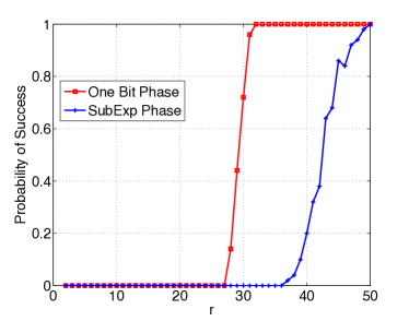
In Figure 1, we report the empirical probability of success of each algorithm for increasing number of measurements r𝑟r. We have a success if the error 1|x^r,x0|2<τ1superscriptsubscript^𝑥𝑟subscript𝑥02𝜏1-|\left\langle{\hat{x}_{r}},{x_{0}}\right\rangle|^{2}<\tau. We set n=8000,τ=0.07formulae-sequence𝑛8000𝜏0.07n=8000,\tau=0.07 in this experiment. We see that the phase transition for 1bitPhase happens earlier than the one for SubExpPhase, which confirms that One Bit Phase retrieval allows lower sample complexity for a given precision.
Refer to caption
Figure 1: Phase transition comparison of one bit Phase retrieval and SubExp phase Retrieval.

6.1.2 Robustness

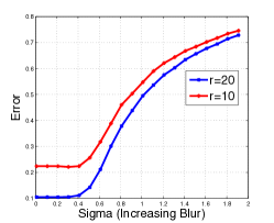
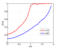
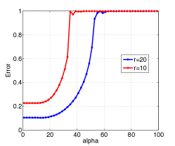
We test the robustness of Algorithm 1 to noise, distortion, and blur. For this end we generate measurements according to the noise model given in Equation (18), for increasing noise level and for r=10𝑟10r=10 and r=20𝑟20r=20. We see in Figure 2(a) that that the recovery error of One Bit Phase Retrieval increases gracefully with the level of noise and as more measurements are available the error of recovery drops down. In the setup of distorted measurements we generate CDP according to Equation (21), for different distortion levels α𝛼\alpha, for different number of measurements r=10𝑟10r=10, and r=20𝑟20r=20. We see in Figure 2(b) that the recovery is still possible thanks to the robustness of One Bit Phase Retrieval, despite the severe non linearity. Finally we test the robustness of 1bitPhase to a gaussian blur with increase aperture. We generate our CDP according to the blurry model in Equation (21), for r=10𝑟10r=10 and r=20𝑟20r=20. We see in Figure 2(c) that phase retrieval ad Super-Resolution are possible with One Bit Phase Retrieval and that the error increases gracefully also with the size of the aperture and drops as more measurements are available.
Refer to caption
(a) Robustness to Exponential noise: Error 1|x,x0|21superscript𝑥subscript𝑥021-|\left\langle{x},{x_{0}}\right\rangle|^{2} versus μ𝜇\mu the mean of the Exponential noise
Refer to caption
(b) Robustness to distortion: Error 1|x,x0|21superscript𝑥subscript𝑥021-|\left\langle{x},{x_{0}}\right\rangle|^{2} versus α𝛼\alpha the size of the clipping.
Refer to caption
(c) Robustness to blur: Error 1|x,x0|21superscript𝑥subscript𝑥021-|\left\langle{x},{x_{0}}\right\rangle|^{2} versus σ𝜎\sigma the aperture of a gaussian filter.
Figure 2: Phase transition comparison of one bit Phase retrieval and SubExp phase Retrieval.

6.1.3 One Bit Phase Retrieval and Alternating Minimization

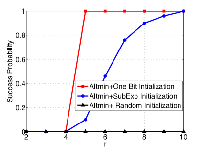
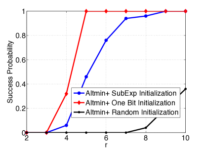
Alternating Minimization Phase Transition. As discussed in Section 2.1.2, and Section 5.3, greedy refinements of the solution of 1bitPhase and SubExpPhase, enhance the quality of the recovery and the sample complexity of the overall procedure as showed in [NJS13] for the Gaussian measurements. Extending those results to Coded Diffraction patterns is subject to future work. We conjecture on one hand that AM initialized with the one bit solution has a sample complexity of O(log3n+log1ϵloglog1ϵ)𝑂superscript3𝑛1italic-ϵ1italic-ϵO(\log^{3}n+\log\frac{1}{\epsilon}\log\log\frac{1}{\epsilon}), and on the other hand that AM initialized with SubExpPhase solution has a sample complexity of O(log5n+log1ϵloglog1ϵ)𝑂superscript5𝑛1italic-ϵ1italic-ϵO(\log^{5}n+\log\frac{1}{\epsilon}\log\log\frac{1}{\epsilon}). We show in the next section the phase transition of AM (Algorithm 3) initialized with 1bitPhase, SubExpPhase and a random initialization in the noisy and the noiseless case.
In order to highlight the effect of the initialization step in the AM Algorithm 3, we fix the number of iterations to t0=50subscript𝑡050t_{0}=50 in the noiseless and the noisy setting.
In figure 3(a) we report the empirical success probability of Algorithm 3 in the noiseless setting versus the number of pairs of modulations r𝑟r. We declare in the noiseless case a success if x^t0x^t0x0x0F<105subscriptnormsubscript^𝑥subscript𝑡0superscriptsubscript^𝑥subscript𝑡0subscript𝑥0superscriptsubscript𝑥0𝐹superscript105||\hat{x}_{t_{0}}\hat{x}_{t_{0}}^{*}-x_{0}x_{0}^{*}||_{F}<10^{-5}. We see that with that relatively small number of iterations, the phase transition of AM initialized with One Bit Phase solution happens at r=4𝑟4r=4. AM initialized with SubExpPhase with that limited number of iterations needs more samples to achieve phase transition at r=10𝑟10r=10. AM initialized at random does not achieve its phase transition with that limited number of samples and iterations. This phase transition confirms the lower sample complexity of one bit solution, and its greedy refinements.
We now turn to the noisy setting (18) where we set σ=0.04𝜎0.04\sigma=0.04. In figure 3(b) we report the empirical success probability of Algorithm 3, where we declare in this setting a success if x^t0x^t0x0x0F<0.03subscriptnormsubscript^𝑥subscript𝑡0superscriptsubscript^𝑥subscript𝑡0subscript𝑥0superscriptsubscript𝑥0𝐹0.03||\hat{x}_{t_{0}}\hat{x}_{t_{0}}^{*}-x_{0}x_{0}^{*}||_{F}<0.03. We see that at that accuracy level, the greedy refinements of one bit solutions are still robust to noise and superior to the other forth-mentioned initializations (SubExpPhase and random).
Refer to caption
(a) Alternating Minimization’s phase transition in the noiseless setting.
Refer to caption
(b) Alternating Minimization’s phase transition in the noisy setting.
Figure 3: Phase transition comparison of one bit Phase retrieval and SubExp phase Retrieval.

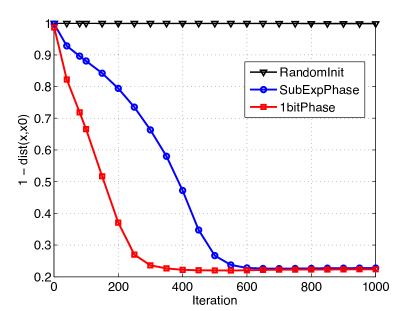
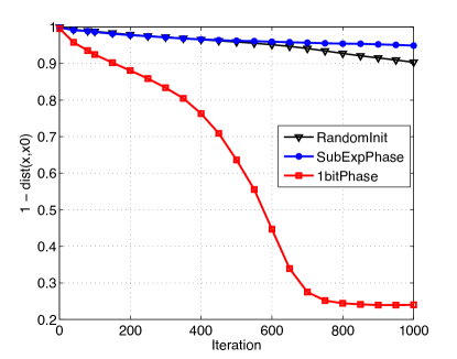
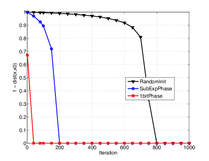
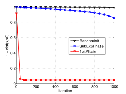
Error Decay. To illustrate the benefit of the initialization step in AM we report in the following the error decay of AM with different initializations. In figure 4(a) we see that in the noiseless setting all approaches converge, the convergence is faster for AM initialized with the one bit solution in high dimension. In figure 4(b)4(c),4(d) we see that AM initialized with one bit solution is more robust in the noisy setting .
Refer to caption
(a) Error 1|x,x0|21superscript𝑥subscript𝑥021-|\left\langle{x},{x_{0}}\right\rangle|^{2} versus Iterations of AltMinPhase, for n=8000𝑛8000n=8000, and a total measurements 8n8𝑛8n in the noiseless setting.
Refer to caption
(b) Error 1|x,x0|21superscript𝑥subscript𝑥021-|\left\langle{x},{x_{0}}\right\rangle|^{2} versus Iterations of AltMinPhase, for n=8000𝑛8000n=8000 and a total measurements 8n8𝑛8n in the noisy setting σ=0.4𝜎0.4\sigma=0.4.
Refer to caption
(c) Error 1|x,x0|21superscript𝑥subscript𝑥021-|\left\langle{x},{x_{0}}\right\rangle|^{2} versus Iterations of AltMinPhase, for n=8000𝑛8000n=8000 and a total measurements 8n8𝑛8n in the noisy setting σ=0.8𝜎0.8\sigma=0.8.
Refer to caption
(d) Error 1|x,x0|21superscript𝑥subscript𝑥021-|\left\langle{x},{x_{0}}\right\rangle|^{2} versus Iterations of AltMinPhase, for n=8000𝑛8000n=8000 and a total measurements 8n8𝑛8n in the noisy setting σ=0.8𝜎0.8\sigma=0.8
Figure 4: Alternating minimization convergence with different initializations: Random Initialization,1bitPhase,and SubExpPhase, in the noisy and noiseless setting.

In the next section we test our algorithms in imaging applications, which highlights the efficiency and the robustness of the algorithms in potential applications in microscopy, astronomy and X-ray Crystallography.

6.2 Imaging Applications

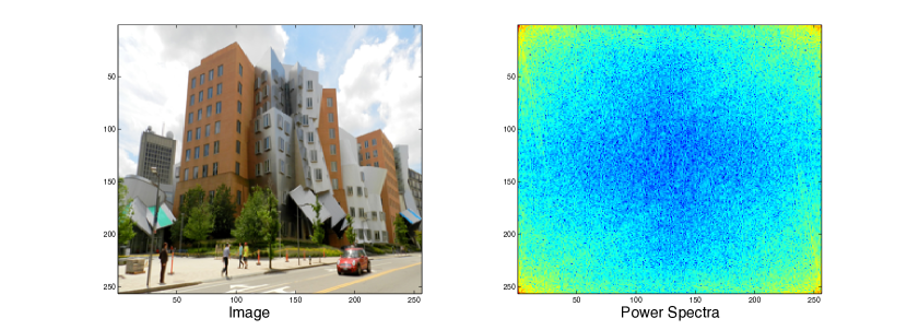
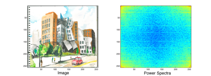
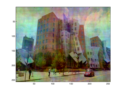
We address in this section the problem of phase recovery in imaging applications. In the following we consider two test images, and their respective power spectra. The image in Figure 5 has a dominant edge structure, and the image in Figure 6 has a dominant textured content . We show that the same algorithms presented in this paper allow the phase recovery, where we simply replace the vectors with 2D2𝐷2D arrays and the 1D1𝐷1D FFT with the 2D2𝐷2D FFT.

Refer to caption
Figure 5: An image of Stata Center (Structured) and its Power Spectra (we plot the logarithm of the power spectra of one color Channel (R for instance) ).
Refer to caption
Figure 6: A drawing of Stata Center (texture like image) and its Power Spectra (we plot the logarithm of the power spectra of one color Channel (R for instance) ).

6.2.1 One Bit Coded Diffraction Patterns

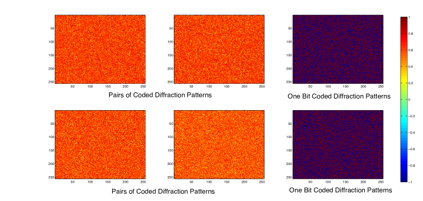
We modulate the image with a 2D2𝐷2D Gaussian array and collect 2D2𝐷2D coded diffraction patterns. We illustrate in Figure 7 the one bit coded diffraction patterns that become in this case a 2D2𝐷2D binary array. The one bit array is obtained by quantizing pairs of coded diffraction arrays. Our goal is therefore to recover robustly the image from the knowledge of One bit coded diffraction arrays using the same algorithms presented in this paper. In the next section we test the robustness of the recovery against distortion, noise and blur.
Refer to caption
Figure 7: One Bit Coded Diffraction Patterns obtained by quantizing pairs of coded diffractions patterns.

6.2.2 Phase Retrieval from Distorted Diffraction Patterns.

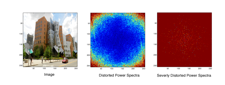
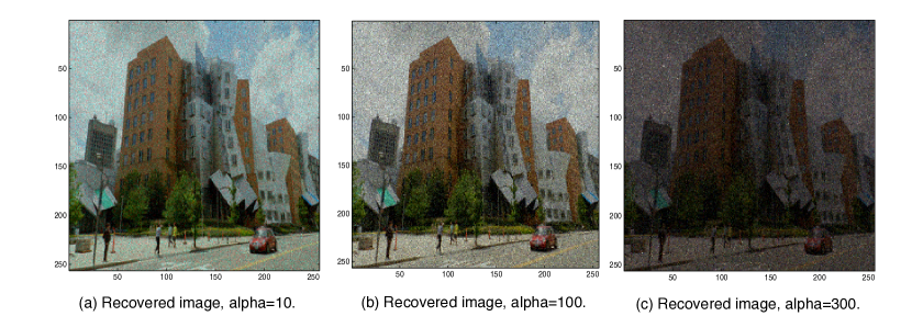
In many acquisition systems we collect the power spectra of an object of interest. This acquisition might be altered by many imperfections due to multiple scattering phenomena for instance, or distortion in the precision of the CCD. Robustness to distortion such as clipping is a desirable feature in phase retrieval. In Figure 8 we simulate distorted power spectra by applying a sigmoid (tanh(α.))(\tanh(\alpha.)) to the Fourier spectrum, for different clipping levels (α𝛼\alpha). While most of the spatial frequency information is lost, phase retrieval is still possible thanks to the robustness of One Bit Phase retrieval to distortions. We apply 2r2𝑟2r Gaussian masks to our image of interest and then collect the power spectra of each masked image. We apply to each masked power spectra a sigmoid with a clipping parameter α𝛼\alpha. We the get our One Bit CDP by quantizing pairs of distorted power spectras. In our experiment n=256×256𝑛256256n=256\times 256, r=16log(n)𝑟16𝑛r=16\lfloor\log(n)\rfloor.

Refer to caption
Figure 8: Stata Center’s power spectra undergoing a distortion such as clipping of the values tanh(α|x^(w)|)𝑡𝑎𝑛𝛼^𝑥𝑤tanh(\alpha|\hat{x}(w)|). The distorted power spectra is obtained for α=0.001𝛼0.001\alpha=0.001. The severely distorted is obtained for α=0.1𝛼0.1\alpha=0.1.
Refer to caption
Figure 9: One Bit Phase Retrieval from distorted CDP. (a) and (b) Recovery from small distortions. (c) Recovery from Severe Distortions.

We run independently the same process of acquisition on the three color channels, as well as Algorithm 1. In Figures 9 and 10 we show the output of the Algorithm 1 for various level of distortions varying from mild to sever distortion. We see that the reconstruction in both cases is still possible from one bit CDP despite the distortion that the intensities values are undergoing.

Refer to caption
Figure 10: One Bit Phase Retrieval from distorted CDP. (a) and (b) Recovery from small distortions. (c) Recovery from Severe Distortions.

6.2.3 Super-Resolution and Blind Deconvolution

We turn now to the problem of recovering an image from its lower end of power spectra. As discussed earlier this is a problem of practical interest in microscopy, as the resolution of an optical system, for instance a lens hh is limited by the Fraunhofer diffraction limit fcsubscript𝑓𝑐f_{c}. The super-resolution factor of hh is therefore defined as SRF=n2fc+1𝑆𝑅𝐹𝑛2subscript𝑓𝑐1SRF=\frac{n}{2f_{c}+1}. In our setup the modulated object diffracts through a lens characterized by a PSF hh and a cut-off frequency fcsubscript𝑓𝑐f_{c}. Hence instead of observing the power spectra of the modulated signal Diag(w)x0𝐷𝑖𝑎𝑔𝑤subscript𝑥0Diag(w)x_{0} we observe the power spectra of a lower resolution signal namely h(Diag(w)x0)𝐷𝑖𝑎𝑔𝑤subscript𝑥0h\star(Diag(w)x_{0}). We consider in this experiment hh to be an averaging filter. In Figure 11(a) we see a blurred image, obtained by convolving the original image Stata with an averaging filter of size 8×8888\times 8. In the following we simulate the diffraction patterns of the modulated image through the aperture hh by taking:(|Fh(Diag(wi1)x0)|2,|Fh(Diag(wi2)x0)|2),i=1rsuperscript𝐹𝐷𝑖𝑎𝑔subscriptsuperscript𝑤1𝑖subscript𝑥02superscript𝐹𝐷𝑖𝑎𝑔subscriptsuperscript𝑤2𝑖subscript𝑥02𝑖1𝑟(|Fh\star(Diag(w^{1}_{i})x_{0})|^{2},|Fh\star(Diag(w^{2}_{i})x_{0})|^{2}),i=1\dots r. We then obtain the one bit CDP by quantizing pairs of CDPs. In our experiment we have n=256×256𝑛256256n=256\times 256, r=10log(n)𝑟10𝑛r=10\lfloor\log(n)\rfloor.
In Figure 11(b), we show the output of Algorithm 1 given the one bit CDP collected as mentioned previously. We see that most of the missing details in Figure 11(a) are recovered. Hence one bit phase retrieval enables super-resolution and blind deconvolution as it is agnostic to the nature of the blur.
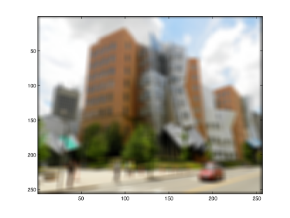
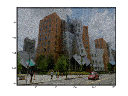
Refer to caption
(a) Image convolved with an averaging filter of size 8×8888\times 8.
Refer to caption
(b) Recovered image from One Bit CDP .
Figure 11: Super-Resolution and Blind Deconvolution via Phase Retrieval from One Bit CDP.

6.2.4 One Bit Phase Retrieval and Alternating Minimization

In this section we test the alternating minimization Algorithm 3 initialized with One Bit Phase Retrieval (Algorithm 1), in the noiseless and the Poisson noise model of equation (19). To emphasis the effect of the initialization we set the number of iterations t0subscript𝑡0t_{0} in Algorithm 3 to a relatively small number. In our experiments we set t0=50subscript𝑡050t_{0}=50, and r=4𝑟4r=4. We test our algorithms with Complex Gaussian masks and Bernoulli masks.

Gaussian masks. We start by the recovery for a noiseless acquisition of the CDP, the recovered image with alternating minimization initialized with one bit phase retrieval is given in Figure 12(a) and is indistinguishable from the original. The average SNR on the three color channels is 101.2248 dB101.2248 dB101.2248\text{ dB}. When the CDP are contaminated with a poisson noise (In Equation (19) we set η=0.1𝜂0.1\eta=0.1 ), Alternating minimization initialized with one bit phase retrieval succeeds and produces a solution with an average SNR on the three color channels of 95.625 dB95.625 dB95.625\text{ dB}. The recovered image in this setting is shown Figure 12(b).

Bernoulli masks. We repeat the same experiment with bernoulli masks , i.e each entry of the mask is a bernoulli random variable with parameter p=0.8𝑝0.8p=0.8. The Recovered image in the noiseless is given in Figure 13(a), the average SNR is 97 dB97 dB97\text{ dB}. In the poisson noise setting the recovered image is given in Figure 13(b), the average SNR is 95.0769 dB95.0769 dB95.0769\text{ dB}. We see that the quality for this fixed number of masks and iterations is lower than the Gaussian case.
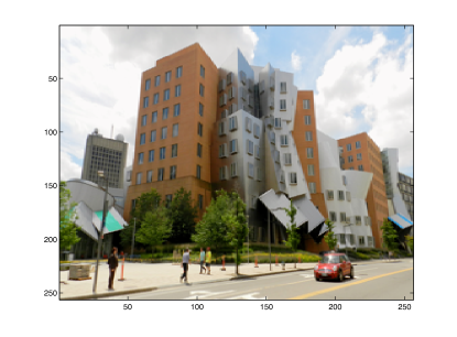
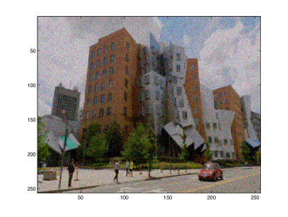
Refer to caption
(a) Recovered Image with AM initialized with the 1bitPhase solution, for a noiseless acquisition of CDP.
Refer to caption
(b) Recovered Image with AM initialized with the 1bitPhase solution, for an acquisition where the CDP are contaminated with a Poisson Noise.
Figure 12: Alternating Minimization and One Bit Phase Retrieval from Gaussian masks.
Refer to caption
(a) Recovered Image with AM initialized with the 1bitPhase solution, for a noiseless acquisition of CDP.
Refer to caption
(b) Recovered Image with AM initialized with the 1bitPhase solution, for an acquisition where the CDP are contaminated with a Poisson Noise.
Figure 13: Alternating Minimization and One Bit Phase Retrieval from Bernoulli masks.

7 Acknowledgements

I am thankful for fruitful discussions with Tomaso Poggio, Lorenzo Rosasco and Gadi Geiger. I would like also to thank Gordon Wetzstein for pointing out reference [ZHY13] and for inspiring discussions on Super-Resolution and applications in microscopy. I am also thankful to Chiyuan Zhang for providing his drawing of Stata center.

8 Proofs

In this section we give the proofs of Proposition 2, Lemma 1 and Proposition 3. We start with the following observation:

Lemma 3.

Let yn𝑦superscript𝑛y\in\mathbb{C}^{n}, and Mn×n𝑀superscript𝑛𝑛M\in\mathbb{C}^{n\times n}, we have the following equality:

y,diag(M)=Tr(Diag(y)M).𝑦𝑑𝑖𝑎𝑔𝑀𝑇𝑟𝐷𝑖𝑎𝑔superscript𝑦𝑀\left\langle{y},{diag(M)}\right\rangle=Tr(Diag(y)^{*}M). (40)

We need this result for yn𝑦superscript𝑛y\in\mathbb{R}^{n}:

y,diag(M)=Tr(Diag(y)M).𝑦𝑑𝑖𝑎𝑔𝑀𝑇𝑟𝐷𝑖𝑎𝑔𝑦𝑀\left\langle{y},{diag(M)}\right\rangle=Tr(Diag(y)M). (41)

Let v=FDiag(w)x𝑣superscript𝐹𝐷𝑖𝑎𝑔superscript𝑤𝑥v=F^{*}Diag(w^{*})x and u=FDiag(w)x0𝑢superscript𝐹𝐷𝑖𝑎𝑔superscript𝑤subscript𝑥0u=F^{*}Diag(w^{*})x_{0}. The proof of proposition 1 follows from Lemmas 4 and 5:

Lemma 4.

The modulus vector can be rewritten in the following way:

|FDiag(w)x|2=diag{FDiag(w)xxDiag(w)F}=diag(vv).superscript𝐹𝐷𝑖𝑎𝑔𝑤𝑥2𝑑𝑖𝑎𝑔superscript𝐹𝐷𝑖𝑎𝑔superscript𝑤𝑥superscript𝑥𝐷𝑖𝑎𝑔𝑤𝐹𝑑𝑖𝑎𝑔𝑣superscript𝑣|FDiag(w)x|^{2}=diag\left\{F^{*}Diag(w^{*})xx^{*}Diag(w)F\right\}=diag(vv^{*}).
Lemma 5.

The following equation holds :

y,|FDiag(w)x|2=xDiag(w)FDiag(y)FDiag(w)x.𝑦superscript𝐹𝐷𝑖𝑎𝑔𝑤𝑥2superscript𝑥𝐷𝑖𝑎𝑔𝑤𝐹𝐷𝑖𝑎𝑔𝑦superscript𝐹𝐷𝑖𝑎𝑔superscript𝑤𝑥\left\langle{y},{|FDiag(w)x|^{2}}\right\rangle=x^{*}Diag(w)FDiag(y)F^{*}Diag(w^{*})x.
Proof of Proposition 1.

By Lemma 5

x0(x)superscriptsubscript𝑥0𝑥\displaystyle\mathcal{E}^{x_{0}}(x) =\displaystyle= 𝔼(y,|FDiag(w1)x|2|FDiag(w2)x|2)𝔼𝑦superscript𝐹𝐷𝑖𝑎𝑔superscript𝑤1𝑥2superscript𝐹𝐷𝑖𝑎𝑔superscript𝑤2𝑥2\displaystyle\mathbb{E}(\left\langle{y},{|FDiag(w^{1})x|^{2}-|FDiag(w^{2})x|^{2}}\right\rangle)
=\displaystyle= xCx.superscript𝑥𝐶𝑥\displaystyle x^{*}Cx.

where C=𝔼(Diag(w1)FDiag(y)FDiag(w1,)Diag(w2)FDiag(y)FDiag(w2,))𝐶𝔼𝐷𝑖𝑎𝑔superscript𝑤1𝐹𝐷𝑖𝑎𝑔𝑦superscript𝐹𝐷𝑖𝑎𝑔superscript𝑤1𝐷𝑖𝑎𝑔superscript𝑤2𝐹𝐷𝑖𝑎𝑔𝑦superscript𝐹𝐷𝑖𝑎𝑔superscript𝑤2C=\mathbb{E}\left(Diag(w^{1})FDiag(y)F^{*}Diag(w^{1,*})-Diag(w^{2})FDiag(y)F^{*}Diag(w^{2,*})\right). ∎

Proof of Lemma 4 .
|FDiag(w)x|2[i]=jFijwjxjkF¯ikwk¯x¯k=jkFijF¯ikwk¯wjxjx¯k.superscript𝐹𝐷𝑖𝑎𝑔𝑤𝑥2delimited-[]𝑖subscript𝑗subscript𝐹𝑖𝑗subscript𝑤𝑗subscript𝑥𝑗subscript𝑘subscript¯𝐹𝑖𝑘¯subscript𝑤𝑘subscript¯𝑥𝑘subscript𝑗𝑘subscript𝐹𝑖𝑗subscript¯𝐹𝑖𝑘¯subscript𝑤𝑘subscript𝑤𝑗subscript𝑥𝑗subscript¯𝑥𝑘|FDiag(w)x|^{2}[i]=\sum_{j}F_{ij}w_{j}x_{j}\sum_{k}\bar{F}_{ik}\bar{w_{k}}\bar{x}_{k}=\sum_{jk}F_{ij}\bar{F}_{ik}\bar{w_{k}}w_{j}x_{j}\bar{x}_{k}. (42)

On the other hand:

eiFDiag(w)xxDiag(w)Fei=[F¯i1Fin¯]𝒲[Fi1Fin],superscriptsubscript𝑒𝑖superscript𝐹𝐷𝑖𝑎𝑔superscript𝑤𝑥superscript𝑥𝐷𝑖𝑎𝑔𝑤𝐹subscript𝑒𝑖delimited-[]subscript¯𝐹𝑖1¯subscript𝐹𝑖𝑛𝒲superscriptdelimited-[]subscript𝐹𝑖1subscript𝐹𝑖𝑛e_{i}^{*}F^{*}Diag(w^{*})xx^{*}Diag(w)Fe_{i}=[\bar{F}_{i1}\dots\bar{F_{in}}]\mathcal{W}[F_{i1}\dots F_{in}]^{\prime}, (43)

where 𝒲jk=wjw¯kxjx¯ksubscript𝒲𝑗𝑘subscript𝑤𝑗subscript¯𝑤𝑘subscript𝑥𝑗subscript¯𝑥𝑘\mathcal{W}_{jk}=w_{j}\bar{w}_{k}x_{j}\bar{x}_{k}. Hence :

eiFDiag(w)xxDiag(w)Fei=jkFijF¯ikwk¯wjxjx¯k.superscriptsubscript𝑒𝑖superscript𝐹𝐷𝑖𝑎𝑔superscript𝑤𝑥superscript𝑥𝐷𝑖𝑎𝑔𝑤𝐹subscript𝑒𝑖subscript𝑗𝑘subscript𝐹𝑖𝑗subscript¯𝐹𝑖𝑘¯subscript𝑤𝑘subscript𝑤𝑗subscript𝑥𝑗subscript¯𝑥𝑘e_{i}^{*}F^{*}Diag(w^{*})xx^{*}Diag(w)Fe_{i}=\sum_{jk}F_{ij}\bar{F}_{ik}\bar{w_{k}}w_{j}x_{j}\bar{x}_{k}. (44)

The lemma is proved. ∎

Proof of Lemma 5.

Using Lemma 3 and Lemma 4,we have:

y,|FDiag(w)x|2𝑦superscript𝐹𝐷𝑖𝑎𝑔𝑤𝑥2\displaystyle\left\langle{y},{|FDiag(w)x|^{2}}\right\rangle =\displaystyle= y,diag{FDiag(w)xxDiag(w)F}𝑦𝑑𝑖𝑎𝑔superscript𝐹𝐷𝑖𝑎𝑔superscript𝑤𝑥superscript𝑥𝐷𝑖𝑎𝑔𝑤𝐹\displaystyle\left\langle{y},{diag\left\{F^{*}Diag(w^{*})xx^{*}Diag(w)F\right\}}\right\rangle
=\displaystyle= Tr(Diag(y)FDiag(w)xxDiag(w)F)𝑇𝑟𝐷𝑖𝑎𝑔𝑦superscript𝐹𝐷𝑖𝑎𝑔superscript𝑤𝑥superscript𝑥𝐷𝑖𝑎𝑔𝑤𝐹\displaystyle Tr(Diag(y)F^{*}Diag(w^{*})xx^{*}Diag(w)F)
=\displaystyle= Tr(Diag(w)FDiag(y)FDiag(w)xx)𝑇𝑟𝐷𝑖𝑎𝑔𝑤𝐹𝐷𝑖𝑎𝑔𝑦superscript𝐹𝐷𝑖𝑎𝑔superscript𝑤𝑥superscript𝑥\displaystyle Tr(Diag(w)FDiag(y)F^{*}Diag(w^{*})xx^{*})
=\displaystyle= xDiag(w)FDiag(y)FDiag(w)x.superscript𝑥𝐷𝑖𝑎𝑔𝑤𝐹𝐷𝑖𝑎𝑔𝑦superscript𝐹𝐷𝑖𝑎𝑔superscript𝑤𝑥\displaystyle x^{*}Diag(w)FDiag(y)F^{*}Diag(w^{*})x.

Proof of Proposition 2.

i-Let v=FDiag(w)x𝑣superscript𝐹𝐷𝑖𝑎𝑔superscript𝑤𝑥v=F^{*}Diag(w^{*})x and u=FDiag(w)x0𝑢superscript𝐹𝐷𝑖𝑎𝑔superscript𝑤subscript𝑥0u=F^{*}Diag(w^{*})x_{0} , visubscript𝑣𝑖v_{i} and ui𝒞𝒩(0,1n),i=1nformulae-sequencesimilar-tosubscript𝑢𝑖𝒞𝒩01𝑛𝑖1𝑛u_{i}\sim\mathcal{C}\mathcal{N}(0,\frac{1}{n}),i=1\dots n. u𝑢u and v𝑣v are gaussian vectors with dependent coordinates. The expectation of dot product u,v𝑢𝑣\left\langle{u},{v}\right\rangle is given in the following:

𝔼(u,v)=𝔼(x0Diag(w)FFDiag(w)x)=x0𝔼(Diag(|w|2))x=x0,x.𝔼𝑢𝑣𝔼superscriptsubscript𝑥0𝐷𝑖𝑎𝑔𝑤𝐹superscript𝐹𝐷𝑖𝑎𝑔superscript𝑤𝑥superscriptsubscript𝑥0𝔼𝐷𝑖𝑎𝑔superscript𝑤2𝑥subscript𝑥0𝑥\mathbb{E}\left(\left\langle{u},{v}\right\rangle\right)=\mathbb{E}\left(x_{0}^{*}Diag(w)FF^{*}Diag(w^{*})x\right)=x_{0}^{*}\mathbb{E}(Diag(|w|^{2}))x=\left\langle{x_{0}},{x}\right\rangle.

since FF=I𝐹superscript𝐹𝐼FF^{*}=I, and 𝔼(Diag(|w|2))=In𝔼𝐷𝑖𝑎𝑔superscript𝑤2subscript𝐼𝑛\mathbb{E}(Diag(|w|^{2}))=I_{n}.
Hence 𝔼(u2)=𝔼(v2)=1𝔼superscriptnorm𝑢2𝔼superscriptnorm𝑣21\mathbb{E}(||u||^{2})=\mathbb{E}(||v||^{2})=1, since x𝑥x and x0subscript𝑥0x_{0} are unitary.
There exists a complex Gaussian random vector r𝑟r, such that each ri𝒞𝒩(0,1n)similar-tosubscript𝑟𝑖𝒞𝒩01𝑛r_{i}\sim\mathcal{C}\mathcal{N}(0,\frac{1}{n}) and risubscript𝑟𝑖r_{i} is independent of uisubscript𝑢𝑖u_{i}, i=1n𝑖1𝑛i=1\dots n and:

v=x0,xu+1|x,x0|2r𝑣subscript𝑥0𝑥𝑢1superscript𝑥subscript𝑥02𝑟v=\left\langle{x_{0}},{x}\right\rangle u+\sqrt{1-|\left\langle{x},{x_{0}}\right\rangle|^{2}}r

Let v1=FDiag(w1,)xsubscript𝑣1superscript𝐹𝐷𝑖𝑎𝑔superscript𝑤1𝑥v_{1}=F^{*}Diag(w^{1,*})x, u1=FDiag(w1,)x0subscript𝑢1superscript𝐹𝐷𝑖𝑎𝑔superscript𝑤1subscript𝑥0u_{1}=F^{*}Diag(w^{1,*})x_{0}, and v2=FDiag(w2,)xsubscript𝑣2superscript𝐹𝐷𝑖𝑎𝑔superscript𝑤2𝑥v_{2}=F^{*}Diag(w^{2,*})x, u2=FDiag(w2,)x0subscript𝑢2superscript𝐹𝐷𝑖𝑎𝑔superscript𝑤2subscript𝑥0u_{2}=F^{*}Diag(w^{2,*})x_{0}. By lemma 4 we have:

x0(x)superscriptsubscript𝑥0𝑥\displaystyle\mathcal{E}^{x_{0}}(x) =\displaystyle= 𝔼(y,|FDiag(w1)x|2|FDiag(w2)x|)𝔼𝑦superscript𝐹𝐷𝑖𝑎𝑔superscript𝑤1𝑥2𝐹𝐷𝑖𝑎𝑔superscript𝑤2𝑥\displaystyle\mathbb{E}\left(\left\langle{y},{|FDiag(w^{1})x|^{2}-|FDiag(w^{2})x|}\right\rangle\right)
=\displaystyle= 𝔼(y,diag(v1v1v2v2))𝔼𝑦𝑑𝑖𝑎𝑔subscript𝑣1superscriptsubscript𝑣1subscript𝑣2superscriptsubscript𝑣2\displaystyle\mathbb{E}(\left\langle{y},{diag(v_{1}v_{1}^{*}-v_{2}v_{2}^{*})}\right\rangle)

On the other hand:

vv𝑣superscript𝑣\displaystyle vv^{*} =\displaystyle= (x0,xu+1|x0,x|2r)(x0,x¯u+1|x0,x|2r)subscript𝑥0𝑥𝑢1superscriptsubscript𝑥0𝑥2𝑟¯subscript𝑥0𝑥superscript𝑢1superscriptsubscript𝑥0𝑥2superscript𝑟\displaystyle(\left\langle{x_{0}},{x}\right\rangle u+\sqrt{1-|\left\langle{x_{0}},{x}\right\rangle|^{2}}r)(\overline{\left\langle{x_{0}},{x}\right\rangle}u^{*}+\sqrt{1-|\left\langle{x_{0}},{x}\right\rangle|^{2}}r^{*})
=\displaystyle= |x0,x|2uu+(1|x,x0|2)rr+21|x0,x|2Re(x0,xur)superscriptsubscript𝑥0𝑥2𝑢superscript𝑢1superscript𝑥subscript𝑥02𝑟superscript𝑟21superscriptsubscript𝑥0𝑥2𝑅𝑒subscript𝑥0𝑥𝑢superscript𝑟\displaystyle|\left\langle{x_{0}},{x}\right\rangle|^{2}uu^{*}+(1-|\left\langle{x},{x_{0}}\right\rangle|^{2})rr^{*}+2\sqrt{1-|\left\langle{x_{0}},{x}\right\rangle|^{2}}Re(\left\langle{x_{0}},{x}\right\rangle ur^{*})

Therefore:

diag(v1v1v2v2)𝑑𝑖𝑎𝑔subscript𝑣1superscriptsubscript𝑣1subscript𝑣2superscriptsubscript𝑣2\displaystyle diag(v_{1}v_{1}^{*}-v_{2}v_{2}^{*}) =\displaystyle= |x0,x|2diag(u1u1u2u2)+(1|x,x0|2)diag(r1r1r2r2)superscriptsubscript𝑥0𝑥2𝑑𝑖𝑎𝑔subscript𝑢1subscriptsuperscript𝑢1subscript𝑢2superscriptsubscript𝑢21superscript𝑥subscript𝑥02𝑑𝑖𝑎𝑔subscript𝑟1superscriptsubscript𝑟1subscript𝑟2superscriptsubscript𝑟2\displaystyle|\left\langle{x_{0}},{x}\right\rangle|^{2}diag(u_{1}u^{*}_{1}-u_{2}u_{2}^{*})+(1-|\left\langle{x},{x_{0}}\right\rangle|^{2})diag(r_{1}r_{1}^{*}-r_{2}r_{2}^{*})
+\displaystyle+ 21|x0,x|2diag(Re(x0,x(u1r1u2r2))\displaystyle 2\sqrt{1-|\left\langle{x_{0}},{x}\right\rangle|^{2}}diag(Re(\left\langle{x_{0}},{x}\right\rangle(u_{1}r^{*}_{1}-u_{2}r_{2}^{*}))
=\displaystyle= |x0,x|2(|FDiag(w1)x0|2|FDiag(w2)x0|2)+(1|x,x0|2)diag(r1r1r2r2)superscriptsubscript𝑥0𝑥2superscript𝐹𝐷𝑖𝑎𝑔superscript𝑤1subscript𝑥02superscript𝐹𝐷𝑖𝑎𝑔superscript𝑤2subscript𝑥021superscript𝑥subscript𝑥02𝑑𝑖𝑎𝑔subscript𝑟1superscriptsubscript𝑟1subscript𝑟2superscriptsubscript𝑟2\displaystyle|\left\langle{x_{0}},{x}\right\rangle|^{2}(|FDiag(w^{1})x_{0}|^{2}-|FDiag(w^{2})x_{0}|^{2})+(1-|\left\langle{x},{x_{0}}\right\rangle|^{2})diag(r_{1}r_{1}^{*}-r_{2}r_{2}^{*})
+\displaystyle+ 21|x0,x|2diag(Re(x0,x(u1r1u2r2)).\displaystyle 2\sqrt{1-|\left\langle{x_{0}},{x}\right\rangle|^{2}}diag(Re(\left\langle{x_{0}},{x}\right\rangle(u_{1}r^{*}_{1}-u_{2}r_{2}^{*})).

Therefore, taking the expectation we have:

x0(x)=|x,x0|2𝔼(y,|FDiag(w1)x0|2|FDiag(w2)x0|2)superscriptsubscript𝑥0𝑥superscript𝑥subscript𝑥02𝔼𝑦superscript𝐹𝐷𝑖𝑎𝑔superscript𝑤1subscript𝑥02superscript𝐹𝐷𝑖𝑎𝑔superscript𝑤2subscript𝑥02\displaystyle\mathcal{E}^{x_{0}}(x)=|\left\langle{x},{x_{0}}\right\rangle|^{2}\mathbb{E}\left(\left\langle{y},{|FDiag(w^{1})x_{0}|^{2}-|FDiag(w^{2})x_{0}|^{2}}\right\rangle\right)

since 𝔼u1,u2y,𝔼r1,r2(diag(r1r1r2r2)|u1,u2)=0subscript𝔼subscript𝑢1subscript𝑢2𝑦subscript𝔼subscript𝑟1subscript𝑟2conditional𝑑𝑖𝑎𝑔subscript𝑟1superscriptsubscript𝑟1subscript𝑟2superscriptsubscript𝑟2subscript𝑢1subscript𝑢20\mathbb{E}_{u_{1},u_{2}}\left\langle{y},{\mathbb{E}_{r_{1},r_{2}}(diag(r_{1}r_{1}^{*}-r_{2}r_{2}^{*})|u_{1},u_{2})}\right\rangle=0,
and 𝔼u1,u2(y,𝔼r1,r2(diag(Re((u1r1u2r2)))|u1,u2))=0subscript𝔼subscript𝑢1subscript𝑢2𝑦subscript𝔼subscript𝑟1subscript𝑟2conditional𝑑𝑖𝑎𝑔𝑅𝑒subscript𝑢1subscriptsuperscript𝑟1subscript𝑢2superscriptsubscript𝑟2subscript𝑢1subscript𝑢20\mathbb{E}_{u_{1},u_{2}}(\left\langle{y},{\mathbb{E}_{r_{1},r_{2}}(diag(Re((u_{1}r^{*}_{1}-u_{2}r_{2}^{*})))|u_{1},u_{2})}\right\rangle)=0.
Let

λ=𝔼(y,|FDiag(w1)x0|2|FDiag(w2)x0|2).𝜆𝔼𝑦superscript𝐹𝐷𝑖𝑎𝑔superscript𝑤1subscript𝑥02superscript𝐹𝐷𝑖𝑎𝑔superscript𝑤2subscript𝑥02\lambda=\mathbb{E}\left(\left\langle{y},{|FDiag(w^{1})x_{0}|^{2}-|FDiag(w^{2})x_{0}|^{2}}\right\rangle\right).

Let Ei1~=|j=1nFijwjx0,j|2~subscriptsuperscript𝐸1𝑖superscriptsuperscriptsubscript𝑗1𝑛subscript𝐹𝑖𝑗subscript𝑤𝑗subscript𝑥0𝑗2\tilde{E^{1}_{i}}=|\sum_{j=1}^{n}F_{ij}w_{j}x_{0,j}|^{2}, since wjsubscript𝑤𝑗w_{j} is complex Gaussian , j=1nFijwjx0,jsuperscriptsubscript𝑗1𝑛subscript𝐹𝑖𝑗subscript𝑤𝑗subscript𝑥0𝑗\sum_{j=1}^{n}F_{ij}w_{j}x_{0,j} is 𝒞𝒩(0,1n)𝒞𝒩01𝑛\mathcal{C}\mathcal{N}(0,\frac{1}{n}), therefore Ei1~~subscriptsuperscript𝐸1𝑖\tilde{E^{1}_{i}} is exponential with mean 1n1𝑛\frac{1}{n} (since |Fij|2=1superscriptsubscript𝐹𝑖𝑗21|F_{ij}|^{2}=1). Let Ei1subscriptsuperscript𝐸1𝑖E^{1}_{i} be an exponential with mean 1. Ei1~=1nEi1~subscriptsuperscript𝐸1𝑖1𝑛subscriptsuperscript𝐸1𝑖\tilde{E^{1}_{i}}=\frac{1}{n}E^{1}_{i}. It follows that:

λ𝜆\displaystyle\lambda =\displaystyle= 𝔼(y,|FDiag(w1)x0|2|FDiag(w2)x0|2)𝔼𝑦superscript𝐹𝐷𝑖𝑎𝑔superscript𝑤1subscript𝑥02superscript𝐹𝐷𝑖𝑎𝑔superscript𝑤2subscript𝑥02\displaystyle\mathbb{E}\left(\left\langle{y},{|FDiag(w^{1})x_{0}|^{2}-|FDiag(w^{2})x_{0}|^{2}}\right\rangle\right)
=\displaystyle= 1ni=1n𝔼(yi(Ei1Ei2)\displaystyle\frac{1}{n}\sum_{i=1}^{n}\mathbb{E}(y_{i}(E^{1}_{i}-E^{2}_{i})
=\displaystyle= 1nn𝔼(y(E1E2))1𝑛𝑛𝔼𝑦superscript𝐸1superscript𝐸2\displaystyle\frac{1}{n}n\mathbb{E}(y(E^{1}-E^{2}))
=\displaystyle= 𝔼(y(E1E2))𝔼𝑦superscript𝐸1superscript𝐸2\displaystyle\mathbb{E}(y(E^{1}-E^{2}))

Where λ𝜆\lambda is defined for different models in Lemma 2 . ∎

Remark 1.

Similar results hold if we use instead of the DFT F𝐹F any unitary matrix U𝑈U. The value of λ𝜆\lambda would depends on |Uij|2superscriptsubscript𝑈𝑖𝑗2|U_{ij}|^{2}.

Proof of Lemma 2.

i. Noiseless:
λ=𝔼(sign(E1E2)(E1E2))=𝔼(|E1E2|)=1𝜆𝔼𝑠𝑖𝑔𝑛subscript𝐸1subscript𝐸2subscript𝐸1subscript𝐸2𝔼subscript𝐸1subscript𝐸21\lambda=\mathbb{E}(sign(E_{1}-E_{2})(E_{1}-E_{2}))=\mathbb{E}(|E_{1}-E_{2}|)=1, since E1E2Exp(1)similar-tosubscript𝐸1subscript𝐸2𝐸𝑥𝑝1E_{1}-E_{2}\sim Exp(1).
ii.Noisy:
Let y=sign((E1+ν1)(E2+ν2))𝑦𝑠𝑖𝑔𝑛subscript𝐸1subscript𝜈1subscript𝐸2subscript𝜈2y=sign\left((E_{1}+\nu_{1})-(E_{2}+\nu_{2})\right). Let L=E1E2𝐿subscript𝐸1subscript𝐸2L=E_{1}-E_{2}, L𝐿L follows a Laplace distribution with mean 0 and scale parameter 111:

LLaplace(0,1).similar-to𝐿𝐿𝑎𝑝𝑙𝑎𝑐𝑒01L\sim Laplace(0,1).

Let N=ν1ν2𝑁subscript𝜈1subscript𝜈2N=\nu_{1}-\nu_{2}, N𝑁N follows a Laplace distribution, NLaplace(0,1γ)similar-to𝑁𝐿𝑎𝑝𝑙𝑎𝑐𝑒01𝛾N\sim Laplace(0,\frac{1}{\gamma}). It follows that:

λ𝜆\displaystyle\lambda =\displaystyle= 𝔼L,N(sign(L+N)L)subscript𝔼𝐿𝑁𝑠𝑖𝑔𝑛𝐿𝑁𝐿\displaystyle\mathbb{E}_{L,N}\left(sign(L+N)L\right)
=\displaystyle= 𝔼L((12N(NL))L)subscript𝔼𝐿12subscript𝑁𝑁𝐿𝐿\displaystyle\mathbb{E}_{L}\left(\left(1-2\mathbb{P}_{N}(N\leq-L)\right)L\right)
=\displaystyle= 𝔼L((12FN(L))L)subscript𝔼𝐿12subscript𝐹𝑁𝐿𝐿\displaystyle\mathbb{E}_{L}\left((1-2F_{N}(-L))L\right)
=\displaystyle= 𝔼L{(12(12+12sign(L)(1exp(γ|L|))))L}subscript𝔼𝐿121212𝑠𝑖𝑔𝑛𝐿1𝛾𝐿𝐿\displaystyle\mathbb{E}_{L}\left\{\left(1-2\left(\frac{1}{2}+\frac{1}{2}sign(-L)\left(1-\exp(-\gamma|L|)\right)\right)\right)L\right\}
=\displaystyle= 𝔼L(sign(L)(1exp(γ|L|))L)subscript𝔼𝐿𝑠𝑖𝑔𝑛𝐿1𝛾𝐿𝐿\displaystyle\mathbb{E}_{L}(sign(L)(1-\exp(-\gamma|L|))L)
=\displaystyle= 𝔼L|L|(1exp(γ|L|))subscript𝔼𝐿𝐿1𝛾𝐿\displaystyle\mathbb{E}_{L}|L|(1-\exp(-\gamma|L|))
=\displaystyle= 10+zexp(γz)exp(z)𝑑z1superscriptsubscript0𝑧𝛾𝑧𝑧differential-d𝑧\displaystyle 1-\int_{0}^{+\infty}z\exp(-\gamma z)\exp(-z)dz
=\displaystyle= 11(1+γ)2>0.11superscript1𝛾20\displaystyle 1-\frac{1}{(1+\gamma)^{2}}>0.

Let σ=1γ2𝜎1superscript𝛾2\sigma=\frac{1}{\gamma^{2}} be the variance of the exponential noise. We conclude that:

λ=1+2σ(1+σ)2.𝜆12𝜎superscript1𝜎2\lambda=\frac{1+2\sqrt{\sigma}}{(1+\sqrt{\sigma})^{2}}.

iii. Distortion:

y𝑦\displaystyle y =\displaystyle= sign(tanh(αE1)tanh(αE2))𝑠𝑖𝑔𝑛𝛼subscript𝐸1𝛼subscript𝐸2\displaystyle sign(\tanh(\alpha E_{1})-\tanh(\alpha E_{2}))
=\displaystyle= sign(tanh(α(E1E2)))(1tanh(αE1)tanh(αE2)))\displaystyle sign(\tanh(\alpha(E_{1}-E_{2})))\left(1-\tanh(\alpha E_{1})\tanh(\alpha E_{2})\right))
=\displaystyle= sign(tanh(α(E1E2))).sign(1tanh(αE1)tanh(αE2)))\displaystyle sign(\tanh(\alpha(E_{1}-E_{2}))).sign\left(1-\tanh(\alpha E_{1})\tanh(\alpha E_{2})\right))
=\displaystyle= sign(E1E2)sign(1tanh(αE1)tanh(αE2)))\displaystyle sign(E_{1}-E_{2})sign\left(1-\tanh(\alpha E_{1})\tanh(\alpha E_{2})\right))

λ=𝔼(y(E1E2))=𝔼(sign(1tanh(αE1)tanh(αE2))|E1E2|).𝜆𝔼𝑦subscript𝐸1subscript𝐸2𝔼𝑠𝑖𝑔𝑛1𝛼subscript𝐸1𝛼subscript𝐸2subscript𝐸1subscript𝐸2\lambda=\mathbb{E}(y(E_{1}-E_{2}))=\mathbb{E}\left(sign\left(1-\tanh(\alpha E_{1})\tanh(\alpha E_{2})\right)|E_{1}-E_{2}|\right).

Proof of Lemma 1.

For xn,x=1formulae-sequence𝑥superscript𝑛norm𝑥1x\in\mathbb{C}^{n},||x||=1, let x0(x)=xCxsuperscriptsubscript𝑥0𝑥superscript𝑥𝐶𝑥\mathcal{E}^{x_{0}}(x)=x^{*}Cx, and ^x0(x)=xC^rxsuperscript^subscript𝑥0𝑥superscript𝑥subscript^𝐶𝑟𝑥\hat{\mathcal{E}}^{x_{0}}(x)=x^{*}\hat{C}_{r}x.

x0(x0)x0(x)=λλ|x0,x|2=λ2xxx0x0F2.superscriptsubscript𝑥0subscript𝑥0superscriptsubscript𝑥0𝑥𝜆𝜆superscriptsubscript𝑥0𝑥2𝜆2subscriptsuperscriptnorm𝑥superscript𝑥subscript𝑥0superscriptsubscript𝑥02𝐹\mathcal{E}^{x_{0}}(x_{0})-\mathcal{E}^{x_{0}}(x)=\lambda-\lambda|\left\langle{x_{0}},{x}\right\rangle|^{2}=\frac{\lambda}{2}||xx^{*}-x_{0}x_{0}^{*}||^{2}_{F}.

Let x^r=argmaxx,x=1^x0(x)subscript^𝑥𝑟subscriptargmax𝑥norm𝑥1superscript^subscript𝑥0𝑥\hat{x}_{r}=\operatornamewithlimits{arg\,max}_{x,||x||=1}\hat{\mathcal{E}}^{x_{0}}(x), we have:

x0(x0)x0(x^r)=x0(x0)^x0(x0)+^x0(x0)^x0(x^r)+^x0(x^r)x0(x^r).superscriptsubscript𝑥0subscript𝑥0superscriptsubscript𝑥0subscript^𝑥𝑟superscriptsubscript𝑥0subscript𝑥0superscript^subscript𝑥0subscript𝑥0superscript^subscript𝑥0subscript𝑥0superscript^subscript𝑥0subscript^𝑥𝑟superscript^subscript𝑥0subscript^𝑥𝑟superscriptsubscript𝑥0subscript^𝑥𝑟\mathcal{E}^{x_{0}}(x_{0})-\mathcal{E}^{x_{0}}(\hat{x}_{r})=\mathcal{E}^{x_{0}}(x_{0})-\hat{\mathcal{E}}^{x_{0}}(x_{0})+\hat{\mathcal{E}}^{x_{0}}(x_{0})-\hat{\mathcal{E}}^{x_{0}}(\hat{x}_{r})+\hat{\mathcal{E}}^{x_{0}}(\hat{x}_{r})-\mathcal{E}^{x_{0}}(\hat{x}_{r}).

Noticing that the term ^x0(x0)^x0(x^r)superscript^subscript𝑥0subscript𝑥0superscript^subscript𝑥0subscript^𝑥𝑟\hat{\mathcal{E}}^{x_{0}}(x_{0})-\hat{\mathcal{E}}^{x_{0}}(\hat{x}_{r}) is non-positive in light of the definition of x^rsubscript^𝑥𝑟\hat{x}_{r}, we have finally: x0(x0)x0(x^r)2supx,x=1^x0(x)x0(x)=2C^rCsuperscriptsubscript𝑥0subscript𝑥0superscriptsubscript𝑥0subscript^𝑥𝑟2subscriptsupremum𝑥norm𝑥1superscript^subscript𝑥0𝑥superscriptsubscript𝑥0𝑥2normsubscript^𝐶𝑟𝐶\mathcal{E}^{x_{0}}(x_{0})-\mathcal{E}^{x_{0}}(\hat{x}_{r})\leq 2\sup_{x,||x||=1}\hat{\mathcal{E}}^{x_{0}}(x)-\mathcal{E}^{x_{0}}(x)=2\left|\left|\hat{C}_{r}-C\right|\right|. Finally:

λ2x^rx^rx0x0F2=x0(x0)x0(x^r)2supx,x=1^x0(x)x0(x)=2C^rC𝜆2subscriptsuperscriptnormsubscript^𝑥𝑟subscriptsuperscript^𝑥𝑟subscript𝑥0superscriptsubscript𝑥02𝐹superscriptsubscript𝑥0subscript𝑥0superscriptsubscript𝑥0subscript^𝑥𝑟2subscriptsupremum𝑥norm𝑥1superscript^subscript𝑥0𝑥superscriptsubscript𝑥0𝑥2normsubscript^𝐶𝑟𝐶\frac{\lambda}{2}||\hat{x}_{r}\hat{x}^{*}_{r}-x_{0}x_{0}^{*}||^{2}_{F}=\mathcal{E}^{x_{0}}(x_{0})-\mathcal{E}^{x_{0}}(\hat{x}_{r})\leq 2\sup_{x,||x||=1}\mathcal{\hat{E}}^{x_{0}}(x)-\mathcal{E}^{x_{0}}(x)=2\left|\left|\hat{C}_{r}-C\right|\right| (45)

Proof of Proposition 3.

It follows that:

𝔼(C^r)=λx0x0𝔼subscript^𝐶𝑟𝜆subscript𝑥0superscriptsubscript𝑥0\mathbb{E}(\hat{C}_{r})=\lambda x_{0}x_{0}^{*}

Where C^r=1ri=1rAisubscript^𝐶𝑟1𝑟superscriptsubscript𝑖1𝑟subscript𝐴𝑖\hat{C}_{r}=\frac{1}{r}\sum_{i=1}^{r}A_{i} where Ai=Diag(wi1)FDiag(yi)FDiag(wi1,)Diag(wi2)FDiag(yi)FDiag(wi2,)subscript𝐴𝑖𝐷𝑖𝑎𝑔subscriptsuperscript𝑤1𝑖𝐹𝐷𝑖𝑎𝑔subscript𝑦𝑖superscript𝐹𝐷𝑖𝑎𝑔subscriptsuperscript𝑤1𝑖𝐷𝑖𝑎𝑔subscriptsuperscript𝑤2𝑖𝐹𝐷𝑖𝑎𝑔subscript𝑦𝑖superscript𝐹𝐷𝑖𝑎𝑔subscriptsuperscript𝑤2𝑖A_{i}=Diag(w^{1}_{i})FDiag(y_{i})F^{*}Diag(w^{1,*}_{i})-Diag(w^{2}_{i})FDiag(y_{i})F^{*}Diag(w^{2,*}_{i})i=1r𝑖1𝑟i=1\dots r.
By Lemma 1, it is now clear that the sample complexity is governed by the concentration of C^rsubscript^𝐶𝑟\hat{C}_{r} around its mean. Let Eβ={wn,|wj1|22βlog(n) and |wj2|22βlog(n),j=1n}.E_{\beta}=\{w\in\mathbb{C}^{n},|w^{1}_{j}|^{2}\leq 2\beta\log(n)\text{ and }|w^{2}_{j}|^{2}\leq 2\beta\log(n),j=1\dots n\}. Let (wi1,wi2),i=1rsubscriptsuperscript𝑤1𝑖subscriptsuperscript𝑤2𝑖𝑖1𝑟(w^{1}_{i},w^{2}_{i}),i=1\dots r, be 2r2𝑟2r independent iid 𝒞𝒩(0,In)𝒞𝒩0subscript𝐼𝑛\mathcal{C}\mathcal{N}(0,I_{n}). Define (w~i1,w~i2)=(wi1,wi2)subscriptsuperscript~𝑤1𝑖subscriptsuperscript~𝑤2𝑖subscriptsuperscript𝑤1𝑖subscriptsuperscript𝑤2𝑖(\tilde{w}^{1}_{i},\tilde{w}^{2}_{i})=(w^{1}_{i},w^{2}_{i}) if (wi1,wi2)Eβsubscriptsuperscript𝑤1𝑖subscriptsuperscript𝑤2𝑖subscript𝐸𝛽(w^{1}_{i},w^{2}_{i})\in E_{\beta} and (w~i1,w2~i)=(0,0)subscriptsuperscript~𝑤1𝑖subscript~superscript𝑤2𝑖00(\tilde{w}^{1}_{i},\tilde{w^{2}}_{i})=(0,0) elsewhere.
Define C~r=1ri=1rA~isubscript~𝐶𝑟1𝑟superscriptsubscript𝑖1𝑟subscript~𝐴𝑖\tilde{C}_{r}=\frac{1}{r}\sum_{i=1}^{r}\tilde{A}_{i}, where

Ai~=Diag(w~i1)FDiag(y~i)FDiag(w~i1,)Diag(w~i2)FDiag(y~i)FDiag(w~i2,),~subscript𝐴𝑖𝐷𝑖𝑎𝑔subscriptsuperscript~𝑤1𝑖𝐹𝐷𝑖𝑎𝑔subscript~𝑦𝑖superscript𝐹𝐷𝑖𝑎𝑔subscriptsuperscript~𝑤1𝑖𝐷𝑖𝑎𝑔subscriptsuperscript~𝑤2𝑖𝐹𝐷𝑖𝑎𝑔subscript~𝑦𝑖superscript𝐹𝐷𝑖𝑎𝑔subscriptsuperscript~𝑤2𝑖\tilde{A_{i}}=Diag(\tilde{w}^{1}_{i})FDiag(\tilde{y}_{i})F^{*}Diag(\tilde{w}^{1,*}_{i})-Diag(\tilde{w}^{2}_{i})FDiag(\tilde{y}_{i})F^{*}Diag(\tilde{w}^{2,*}_{i}),

and let C~=𝔼C~r~𝐶𝔼subscript~𝐶𝑟\tilde{C}=\mathbb{E}\tilde{C}_{r}. By the triangular inequality we have:

C^rCC^rC~r+C~rC~+C~Cnormsubscript^𝐶𝑟𝐶normsubscript^𝐶𝑟subscript~𝐶𝑟normsubscript~𝐶𝑟~𝐶norm~𝐶𝐶\left|\left|\hat{C}_{r}-C\right|\right|\leq\left|\left|\hat{C}_{r}-\tilde{C}_{r}\right|\right|+\left|\left|\tilde{C}_{r}-\tilde{C}\right|\right|+\left|\left|\tilde{C}-C\right|\right| (46)

Bounding C^rC~rnormsubscript^𝐶𝑟subscript~𝐶𝑟\left|\left|\hat{C}_{r}-\tilde{C}_{r}\right|\right|:
Note that C^rC~r=0normsubscript^𝐶𝑟subscript~𝐶𝑟0\left|\left|\hat{C}_{r}-\tilde{C}_{r}\right|\right|=0, if for all i=1r𝑖1𝑟i=1\dots r, (wi1,wi2)Eβsubscriptsuperscript𝑤1𝑖subscriptsuperscript𝑤2𝑖subscript𝐸𝛽(w^{1}_{i},w^{2}_{i})\in E_{\beta}. Let us get a bound on the probability of that event. Note that: (|wi|2>2βlog(n))2nβsuperscriptsubscript𝑤𝑖22𝛽𝑛2superscript𝑛𝛽\mathbb{P}(|w_{i}|^{2}>2\beta\log(n))\leq 2n^{-\beta}. To avoid cumbersome notations when we use index i𝑖i, wisubscript𝑤𝑖w_{i} refers to a modulation in nsuperscript𝑛\mathbb{C}^{n}, i=1r𝑖1𝑟i=1\dots r, and when we use index j𝑗j wjsubscript𝑤𝑗w_{j} refers to the jth𝑗𝑡j-th component of wn,j=1nformulae-sequence𝑤superscript𝑛𝑗1𝑛w\in\mathbb{C}^{n},j=1\dots n.

{i{1r} such that (wi1,wi2)Eβ}formulae-sequence𝑖1𝑟 such that subscriptsuperscript𝑤1𝑖subscriptsuperscript𝑤2𝑖subscript𝐸𝛽\displaystyle\mathbb{P}\left\{\exists i\in\{1\dots r\}\quad\text{ such that }(w^{1}_{i},w^{2}_{i})\notin E_{\beta}\right\} \displaystyle\leq r{(w1,w2)Eβ}𝑟superscript𝑤1superscript𝑤2subscript𝐸𝛽\displaystyle r\mathbb{P}\left\{(w^{1},w^{2})\notin E_{\beta}\right\}
=\displaystyle= r{j such that |wj1|2>2βlog(n) Or |wj1|2>2βlog(n)}𝑟𝑗 such that superscriptsubscriptsuperscript𝑤1𝑗22𝛽𝑛 Or superscriptsubscriptsuperscript𝑤1𝑗22𝛽𝑛\displaystyle r\mathbb{P}\left\{\exists j\text{ such that }|w^{1}_{j}|^{2}>2\beta\log(n)\text{ Or }|w^{1}_{j}|^{2}>2\beta\log(n)\right\}
\displaystyle\leq 4rnnβ.4𝑟𝑛superscript𝑛𝛽\displaystyle\frac{4rn}{n^{\beta}}.

It follows that:

C^rC~r=0 with probability at least 14rnβ1.normsubscript^𝐶𝑟subscript~𝐶𝑟0 with probability at least 14𝑟superscript𝑛𝛽1\left|\left|\hat{C}_{r}-\tilde{C}_{r}\right|\right|=0\text{ with probability at least }1-\frac{4r}{n^{\beta-1}}. (47)

Bounding C~rC~normsubscript~𝐶𝑟~𝐶\left|\left|\tilde{C}_{r}-\tilde{C}\right|\right|:

Let

X~i=A~i𝔼(A~i),subscript~𝑋𝑖subscript~𝐴𝑖𝔼subscript~𝐴𝑖\tilde{X}_{i}=\tilde{A}_{i}-\mathbb{E}(\tilde{A}_{i}),

𝔼(X~i)=0𝔼subscript~𝑋𝑖0\mathbb{E}(\tilde{X}_{i})=0. Note that

C~rC~=1ri=1rX~inormsubscript~𝐶𝑟~𝐶1𝑟normsuperscriptsubscript𝑖1𝑟subscript~𝑋𝑖\left|\left|\tilde{C}_{r}-\tilde{C}\right|\right|=\frac{1}{r}\left|\left|\sum_{i=1}^{r}\tilde{X}_{i}\right|\right|

Let us get a bound on X~inormsubscript~𝑋𝑖||\tilde{X}_{i}||. Note that 𝔼(Ai~)λnorm𝔼~subscript𝐴𝑖𝜆||\mathbb{E}(\tilde{A_{i}})||\leq\lambda. To simplify the notation we will omit in the following the indices.

A~norm~𝐴\displaystyle\left|\left|\tilde{A}\right|\right| =\displaystyle= supx,x=1y~,|FDiag(w~1)x|2|FDiag(w~2)x|2subscriptsupremum𝑥norm𝑥1~𝑦superscript𝐹𝐷𝑖𝑎𝑔superscript~𝑤1𝑥2superscript𝐹𝐷𝑖𝑎𝑔superscript~𝑤2𝑥2\displaystyle\sup_{x,||x||=1}\left\langle{\tilde{y}},{|FDiag(\tilde{w}^{1})x|^{2}-|FDiag(\tilde{w}^{2})x|^{2}}\right\rangle

Recall that v=FDiag(w~)x𝑣superscript𝐹𝐷𝑖𝑎𝑔superscript~𝑤𝑥v=F^{*}Diag(\tilde{w}^{*})x. Note that: |FDiag(w~)x|2=diag{FDiag(w~)xxDiag(w~)F}=diag(vv)superscript𝐹𝐷𝑖𝑎𝑔~𝑤𝑥2𝑑𝑖𝑎𝑔superscript𝐹𝐷𝑖𝑎𝑔superscript~𝑤𝑥superscript𝑥𝐷𝑖𝑎𝑔~𝑤𝐹𝑑𝑖𝑎𝑔𝑣superscript𝑣|FDiag(\tilde{w})x|^{2}=diag\left\{F^{*}Diag(\tilde{w}^{*})xx^{*}Diag(\tilde{w})F\right\}=diag(vv^{*}).
By holder inequality we have:

y~,|FDiag(w~1)x|2|FDiag(w~2)x|2~𝑦superscript𝐹𝐷𝑖𝑎𝑔superscript~𝑤1𝑥2superscript𝐹𝐷𝑖𝑎𝑔superscript~𝑤2𝑥2\displaystyle\left\langle{\tilde{y}},{|FDiag(\tilde{w}^{1})x|^{2}-|FDiag(\tilde{w}^{2})x|^{2}}\right\rangle =\displaystyle= y~,diag(v1v1,)diag(v2v2,)~𝑦𝑑𝑖𝑎𝑔superscript𝑣1superscript𝑣1𝑑𝑖𝑎𝑔superscript𝑣2superscript𝑣2\displaystyle\left\langle{\tilde{y}},{diag(v^{1}v^{1,*})-diag(v^{2}v^{2,*})}\right\rangle
\displaystyle\leq y~diag(v1v1,)diag(v2v2,)1.subscriptnorm~𝑦subscriptnorm𝑑𝑖𝑎𝑔superscript𝑣1superscript𝑣1𝑑𝑖𝑎𝑔superscript𝑣2superscript𝑣2subscript1\displaystyle||\tilde{y}||_{\infty}\left|\left|diag(v^{1}v^{1,*})-diag(v^{2}v^{2,*})\right|\right|_{\ell_{1}}.

Since y~~𝑦\tilde{y} is binary y~=1subscriptnorm~𝑦1||\tilde{y}||_{\infty}=1. By the triangular inequality:

diag(v1v1,)diag(v2v2,)1diag(v1v1,)1+diag(v2v2,)1.subscriptnorm𝑑𝑖𝑎𝑔superscript𝑣1superscript𝑣1𝑑𝑖𝑎𝑔superscript𝑣2superscript𝑣2subscript1subscriptnorm𝑑𝑖𝑎𝑔superscript𝑣1superscript𝑣1subscript1subscriptnorm𝑑𝑖𝑎𝑔superscript𝑣2superscript𝑣2subscript1\left|\left|diag(v^{1}v^{1,*})-diag(v^{2}v^{2,*})\right|\right|_{\ell_{1}}\leq\left|\left|diag(v^{1}v^{1,*})\right|\right|_{\ell_{1}}+\left|\left|diag(v^{2}v^{2,*})\right|\right|_{\ell_{1}}.
diag(vv)1=|FDiag(w)x|21subscriptnorm𝑑𝑖𝑎𝑔𝑣superscript𝑣subscript1subscriptnormsuperscript𝐹𝐷𝑖𝑎𝑔𝑤𝑥2subscript1\displaystyle\left|\left|diag(vv^{*})\right|\right|_{\ell_{1}}=\left|\left||FDiag(w)x|^{2}\right|\right|_{\ell_{1}} =\displaystyle= diag{FDiag(w~)xxDiag(w~)F}1subscriptnorm𝑑𝑖𝑎𝑔superscript𝐹𝐷𝑖𝑎𝑔superscript~𝑤𝑥superscript𝑥𝐷𝑖𝑎𝑔~𝑤𝐹subscript1\displaystyle||diag\left\{F^{*}Diag(\tilde{w}^{*})xx^{*}Diag(\tilde{w})F\right\}||_{\ell_{1}}
=\displaystyle= Tr(FDiag(w~)xxDiag(w~)F)𝑇𝑟superscript𝐹𝐷𝑖𝑎𝑔superscript~𝑤𝑥superscript𝑥𝐷𝑖𝑎𝑔~𝑤𝐹\displaystyle Tr(F^{*}Diag(\tilde{w}^{*})xx^{*}Diag(\tilde{w})F)
=\displaystyle= Tr(Diag(w~)FFDiag(w~)xx)𝑇𝑟𝐷𝑖𝑎𝑔~𝑤𝐹superscript𝐹𝐷𝑖𝑎𝑔superscript~𝑤𝑥superscript𝑥\displaystyle Tr(Diag(\tilde{w})FF^{*}Diag(\tilde{w}^{*})xx^{*})
=\displaystyle= Tr(Diag(|w~|2)xx)𝑇𝑟𝐷𝑖𝑎𝑔superscript~𝑤2𝑥superscript𝑥\displaystyle Tr(Diag(|\tilde{w}|^{2})xx^{*})
\displaystyle\leq Diag(|w~|2)x2.norm𝐷𝑖𝑎𝑔superscript~𝑤2superscriptnorm𝑥2\displaystyle\left|\left|Diag(|\tilde{w}|^{2})\right|\right|||x||^{2}.

We are now left with Bounding:

supx,x=1(Diag(|w~1|2)+Diag(|w~2|2))x2subscriptsupremum𝑥norm𝑥1norm𝐷𝑖𝑎𝑔superscriptsuperscript~𝑤12norm𝐷𝑖𝑎𝑔superscriptsuperscript~𝑤22superscriptnorm𝑥2\displaystyle\sup_{x,||x||=1}\left(\left|\left|Diag(|\tilde{w}^{1}|^{2})\right|\right|+\left|\left|Diag(|\tilde{w}^{2}|^{2})\right|\right|\right)||x||^{2} =\displaystyle= (Diag(|w~1|2)+Diag(|w~2|2))norm𝐷𝑖𝑎𝑔superscriptsuperscript~𝑤12norm𝐷𝑖𝑎𝑔superscriptsuperscript~𝑤22\displaystyle\left(\left|\left|Diag(|\tilde{w}^{1}|^{2})\right|\right|+\left|\left|Diag(|\tilde{w}^{2}|^{2})\right|\right|\right) (48)
=\displaystyle= maxj=1n|w~j1|2+maxj=1n|w~j2|2subscript𝑗1𝑛superscriptsubscriptsuperscript~𝑤1𝑗2subscript𝑗1𝑛superscriptsubscriptsuperscript~𝑤2𝑗2\displaystyle\max_{j=1\dots n}|\tilde{w}^{1}_{j}|^{2}+\max_{j=1\dots n}|\tilde{w}^{2}_{j}|^{2}

By definition of (w~1,w2~)superscript~𝑤1~superscript𝑤2(\tilde{w}^{1},\tilde{w^{2}}) we conclude that :

A~4βlog(n).norm~𝐴4𝛽𝑛||\tilde{A}||\leq 4\beta\log(n). (49)

It follows that

X~i4βlog(n)+λ5βlog(n):=Δ.normsubscript~𝑋𝑖4𝛽𝑛𝜆5𝛽𝑛assignΔ||\tilde{X}_{i}||\leq 4\beta\log(n)+\lambda\leq 5\beta\log(n):=\Delta.
Theorem 2 (Hoeffding Matrix Inequality [Tro12]).

Let Xi,i=1rsubscript𝑋𝑖𝑖1𝑟X_{i},i=1\dots r be a sequence of independent random n×n𝑛𝑛n\times n self adjoint matrices. Assume that each random matrix obeys:

𝔼(Xi)=0 and XiΔ almost surely.formulae-sequence𝔼subscript𝑋𝑖0 and normsubscript𝑋𝑖Δ almost surely.\mathbb{E}(X_{i})=0\quad\text{ and }||X_{i}||\leq\Delta\text{ almost surely.}

Then for all t0𝑡0t\geq 0,

{1ri=1rXit}2nexp(rt28Δ2).1𝑟normsuperscriptsubscript𝑖1𝑟subscript𝑋𝑖𝑡2𝑛𝑟superscript𝑡28superscriptΔ2\mathbb{P}\left\{\frac{1}{r}\left|\left|\sum_{i=1}^{r}X_{i}\right|\right|\geq t\right\}\leq 2n\exp\left(-\frac{rt^{2}}{8\Delta^{2}}\right).

In other words:

For rt2ϵ2Δ2log(n),1ri=1rXiϵ with probability at least 1nt2.formulae-sequenceFor 𝑟superscript𝑡2superscriptitalic-ϵ2superscriptΔ2𝑛1𝑟normsuperscriptsubscript𝑖1𝑟subscript𝑋𝑖italic-ϵ with probability at least 1superscript𝑛superscript𝑡2\text{For }r\geq\frac{t^{2}}{\epsilon^{2}}\Delta^{2}\log(n),\quad\frac{1}{r}\left|\left|\sum_{i=1}^{r}X_{i}\right|\right|\leq\epsilon\text{ with probability at least }1-n^{-t^{2}}.

We are now ready to apply the Hoeffding Matrix inequality:

For rct2ϵ2β2log3n,1ri=1rX~iϵ with probability at least 1nt2.formulae-sequenceFor 𝑟𝑐superscript𝑡2superscriptitalic-ϵ2superscript𝛽2superscript3𝑛1𝑟normsuperscriptsubscript𝑖1𝑟subscript~𝑋𝑖italic-ϵ with probability at least 1superscript𝑛superscript𝑡2\text{For }r\geq c\frac{t^{2}}{\epsilon^{2}}\beta^{2}\log^{3}n,\quad\frac{1}{r}\left|\left|\sum_{i=1}^{r}\tilde{X}_{i}\right|\right|\leq\epsilon\text{ with probability at least }1-n^{-t^{2}}.

It follows that:

For C~rC~ctβlog3nr with probability at least 1nt2.For normsubscript~𝐶𝑟~𝐶𝑐𝑡𝛽superscript3𝑛𝑟 with probability at least 1superscript𝑛superscript𝑡2\text{For }\left|\left|\tilde{C}_{r}-\tilde{C}\right|\right|\leq ct\beta\sqrt{\frac{\log^{3}n}{r}}\text{ with probability at least }1-n^{-t^{2}}. (50)

Bounding C~Cnorm~𝐶𝐶\left|\left|\tilde{C}-{C}\right|\right|:
By Jensen inequality followed by Cauchy Sharwz inequality we have:

C~Cnorm~𝐶𝐶\displaystyle\left|\left|\tilde{C}-{C}\right|\right| =\displaystyle= 𝔼(1Iw1,w2EβA)norm𝔼1subscriptIsuperscript𝑤1superscript𝑤2subscript𝐸𝛽𝐴\displaystyle\left|\left|\mathbb{E}\left(1{\hskip-2.5pt}\hbox{I}_{w^{1},w^{2}\notin E_{\beta}}A\right)\right|\right|
\displaystyle\leq 𝔼1Iw1,w2EβA𝔼1subscriptIsuperscript𝑤1superscript𝑤2subscript𝐸𝛽norm𝐴\displaystyle\mathbb{E}1{\hskip-2.5pt}\hbox{I}_{w^{1},w^{2}\notin E_{\beta}}\left|\left|A\right|\right|
\displaystyle\leq 𝔼(1Iw1,w2Eβ)E(A2)𝔼1subscriptIsuperscript𝑤1superscript𝑤2subscript𝐸𝛽𝐸superscriptnorm𝐴2\displaystyle\sqrt{\mathbb{E}(1{\hskip-2.5pt}\hbox{I}_{w^{1},w^{2}\notin E_{\beta}})}\sqrt{E(\left|\left|A\right|\right|^{2})}
\displaystyle\leq (Eβc)𝔼(maxj=1n|wj1|2+maxj=1n|wj2|2)2.subscriptsuperscript𝐸𝑐𝛽𝔼superscriptsubscript𝑗1𝑛superscriptsubscriptsuperscript𝑤1𝑗2subscript𝑗1𝑛superscriptsubscriptsuperscript𝑤2𝑗22\displaystyle\sqrt{\mathbb{P}(E^{c}_{\beta})}\sqrt{\mathbb{E}(\max_{j=1\dots n}|w^{1}_{j}|^{2}+\max_{j=1\dots n}|w^{2}_{j}|^{2})^{2}}.

The last inequality follows from equation (48).

A2(maxj=1n|wj1|2)2+(maxj=1n|wj2|2)2+2maxj=1n|wj1|2maxj=1n|wj2|2.superscriptnorm𝐴2superscriptsubscript𝑗1𝑛superscriptsubscriptsuperscript𝑤1𝑗22superscriptsubscript𝑗1𝑛superscriptsubscriptsuperscript𝑤2𝑗222subscript𝑗1𝑛superscriptsubscriptsuperscript𝑤1𝑗2subscript𝑗1𝑛superscriptsubscriptsuperscript𝑤2𝑗2||A||^{2}\leq(\max_{j=1\dots n}|w^{1}_{j}|^{2})^{2}+(\max_{j=1\dots n}|w^{2}_{j}|^{2})^{2}+2\max_{j=1\dots n}|w^{1}_{j}|^{2}\max_{j=1\dots n}|w^{2}_{j}|^{2}. (51)

Let Z=maxj=1nEj,EjExp(1)formulae-sequence𝑍subscript𝑗1𝑛subscript𝐸𝑗similar-tosubscript𝐸𝑗𝐸𝑥𝑝1Z=\max_{j=1\dots n}E_{j},\quad E_{j}\sim Exp(1) iid, therefore:

𝔼(||A||2)2(E(Z2)+(E(Z))2)=2(Var(Z))+2(E(Z))2).\mathbb{E}\left(||A||^{2}\right)\leq 2(E(Z^{2})+(E(Z))^{2})=2(Var(Z))+2(E(Z))^{2}). (52)
Lemma 6 (Maximum of Exponential [BT12]).

Let Z=maxj=1nEj,EjExp(1)formulae-sequence𝑍subscript𝑗1𝑛subscript𝐸𝑗similar-tosubscript𝐸𝑗𝐸𝑥𝑝1Z=\max_{j=1\dots n}E_{j},\quad E_{j}\sim Exp(1) iid, therefore: Var(Z)2𝔼(Z)=i=1n1ilog(n).formulae-sequence𝑉𝑎𝑟𝑍2𝔼𝑍superscriptsubscript𝑖1𝑛1𝑖𝑛Var(Z)\leq 2\quad\mathbb{E}(Z)=\sum_{i=1}^{n}\frac{1}{i}\leq\log(n).

For sufficiently large n𝑛n, there exists a constant c𝑐c such that:

𝔼(A2)2(E(Z2)+(E(Z))2)=2(2+2(log2(n)))=4(1+log2(n))c2log2(n).𝔼superscriptnorm𝐴22𝐸superscript𝑍2superscript𝐸𝑍2222superscript2𝑛41superscript2𝑛superscript𝑐2superscript2𝑛\mathbb{E}\left(||A||^{2}\right)\leq 2(E(Z^{2})+(E(Z))^{2})=2(2+2(\log^{2}(n)))=4(1+\log^{2}(n))\leq c^{2}\log^{2}(n). (53)

Note that (Eβc)4nnβsubscriptsuperscript𝐸𝑐𝛽4𝑛superscript𝑛𝛽\mathbb{P}(E^{c}_{\beta})\leq\frac{4n}{n^{\beta}}. Therefore:

C~C2cn(β1)/2log(n).norm~𝐶𝐶2𝑐superscript𝑛𝛽12𝑛\left|\left|\tilde{C}-{C}\right|\right|\leq\frac{{2}c}{n^{(\beta-1)/2}}\log(n). (54)

Putting all together:
Putting together equations (46),(47),(50) and (54) we have finally with probability at least 1nt24rnβ11superscript𝑛superscript𝑡24𝑟superscript𝑛𝛽11-n^{-t^{2}}-\frac{4r}{n^{\beta-1}}:

C^rCcβtlog3nr+2cn(β1)/2log(n).normsubscript^𝐶𝑟𝐶𝑐𝛽𝑡superscript3𝑛𝑟2𝑐superscript𝑛𝛽12𝑛||\hat{C}_{r}-C||\leq c\beta t\sqrt{\frac{\log^{3}n}{r}}+\frac{{2}c}{n^{(\beta-1)/2}}\log(n). (55)

Setting t=2,β=4formulae-sequence𝑡2𝛽4t=\sqrt{2},\beta=4 we get with probability 1O(n2)1𝑂superscript𝑛21-O(n^{-2}),

C^rC42clog3nr+2cn3/2log(n).normsubscript^𝐶𝑟𝐶42𝑐superscript3𝑛𝑟2𝑐superscript𝑛32𝑛||\hat{C}_{r}-C||\leq 4\sqrt{2}c\sqrt{\frac{\log^{3}n}{r}}+\frac{{2}c}{n^{3/2}}\log(n). (56)

It follows that there exists a numeric constant c𝑐c such that:

For rclog3nϵ2C^rCϵ, with probability at least 1O(n2).formulae-sequenceFor 𝑟𝑐superscript3𝑛superscriptitalic-ϵ2normsubscript^𝐶𝑟𝐶italic-ϵ with probability at least 1𝑂superscript𝑛2\text{For }r\geq c\frac{\log^{3}n}{\epsilon^{2}}\quad||\hat{C}_{r}-C||\leq\epsilon,\text{ with probability at least }1-O(n^{-2}). (57)

Finally by equation (45) we conclude that:

For rclog3nϵ212x^rx^rx0x0F2ϵλ, with probability at least 1O(n2).formulae-sequenceFor 𝑟𝑐superscript3𝑛superscriptitalic-ϵ212subscriptsuperscriptnormsubscript^𝑥𝑟subscriptsuperscript^𝑥𝑟subscript𝑥0superscriptsubscript𝑥02𝐹italic-ϵ𝜆 with probability at least 1𝑂superscript𝑛2\text{For }r\geq c\frac{\log^{3}n}{\epsilon^{2}}\quad\frac{1}{2}||\hat{x}_{r}\hat{x}^{*}_{r}-x_{0}x_{0}^{*}||^{2}_{F}\leq\frac{\epsilon}{\lambda},\text{ with probability at least }1-O(n^{-2}). (58)

In other words for another numeric constant c𝑐c we have:

For rclog3nϵ2λ2x^rx^rx0x0F2ϵ, with probability at least 1O(n2).formulae-sequenceFor 𝑟𝑐superscript3𝑛superscriptitalic-ϵ2superscript𝜆2subscriptsuperscriptnormsubscript^𝑥𝑟subscriptsuperscript^𝑥𝑟subscript𝑥0superscriptsubscript𝑥02𝐹italic-ϵ with probability at least 1𝑂superscript𝑛2\text{For }r\geq c\frac{\log^{3}n}{\epsilon^{2}\lambda^{2}}\quad||\hat{x}_{r}\hat{x}^{*}_{r}-x_{0}x_{0}^{*}||^{2}_{F}\leq\epsilon,\text{ with probability at least }1-O(n^{-2}). (59)

References

  • [ABFM12] B. Alexeev, A. S. Bandeira, M. Fickus, and D. G. Mixon. Phase retrieval with polarization. arXiv preprint arXiv:1210.7752, 12(4):389–434, 2012.
  • [ASBM13] Y. Chen A. S. Bandeira and D. G. Mixon. Phase retrieval from power spectra of masked signals. arXiv preprint arXiv:1303.4458, 2013.
  • [BDP+07] O. Bunk, A. Diaz, F. Pfeiffer, C. David, B. Schmitt, D.K. Satapathy, and JF Veen. Diffractive imaging for periodic samples: retrieving one-dimensional concentration profiles across microfluidic channels. Acta Crystallographica Section A: Foundations of Crystallography, 63(4):306 314, 2007.
  • [BT12] S. Boucheron and M. Thomas. Concentration inequalities for order statistics. Electronic communication in probability., 2012.
  • [CL12] E. J. Candes and X. Li. Solving quadratic equations via phaselift when there are about as many equations as unknowns. To appear in Foundations of Computational Mathematics., 2012.
  • [CLM13] E. Candes, X. Li, and M.Soltanolkotab. Phase retrieval from coded diffraction patterns. arxiv, 2013.
  • [CSV11] E. J. Candes, T. Strohmer, and V. Voroninski. Phaselift : exact and stable signal recovery from magnitude measurements via convex programming. To appear in Communications in Pure and Applied Mathematics, 2011.
  • [DH12] L. Demanet and P. Hand. Stable optimizationless recovery from phaseless linear measurements. arXiv:1208.1803, 2012.
  • [FGC12] C. Fernandez-Granda and E. J. Candes. Towards a mathematical theory of super-resolution. To appear in Communications on Pure and Applied Mathematics, 2012.
  • [Fie82] J.R. Fienup. Phase retrieval algorithms: a comparison. Applied optics,21(15):2758 2769, 1982.
  • [Fri66] D.L Fried. Optical resolution through a randomly inhomogeneous medium for very long and very short exposures. Journal of physics, J. Opt. Soc. Am. 56, 1372-1379, 1966.
  • [GL84] D. Griffin and J. Lim. Signal estimation from modified short-time fourier transform. Acoustics, Speech and Signal Processing, IEEE Transactions on, 32(2):236 243, 1984.
  • [GS72] R. Gerchberg and W. Saxtong. A practical algorithm for the determination of phase from image and diffraction plane pictures. Optik, 35:237 246, 1972.
  • [Gus00] M. G. L. Gustafsson. Surpassing the lateral resolution limit by a factor of two using structured illumination microscopy. Journal of Microscopy, 198, Pt 2, May 2000, pp. 82 87, 2000.
  • [Har93] R.W. Harrison. Phase problem in crystallography. JOSA A, 10(5):1046 1055, 1993.
  • [HKH+13] M.J. Humphry, B. Kraus, A.C. Hurst, A.M. Maiden, and J.M. Rodenburg. Ptychographic electron microscopy using high-angle dark-field scattering for sub-nanometre resolution imaging. Nature, 2013.
  • [Lea08] Y. J Liu and et al. Phase retrieval in x-ray imaging based on using structured illumination. Phys. Rev. A, 78:023817, 2008.
  • [LT91] M Ledoux and M Talagrand. Probability in banach spaces: isoperimetry and processes. Springer-Verlag, 1991.
  • [Mis73] D.L. Misell. A method for the solution of the phase problem in electron microscopy. Journal of physics, 1973.
  • [MISE08] J. Miao, T. Ishikawa, Q. Shen, and T. Earnest. Extending x-ray crystallography to allow the imaging of noncrystalline materials, cells, and single protein complexes. Annu. Rev. Phys. Chem., 59:387 410, 2008.
  • [MR13] Y. Mroueh and L. Rosasco. Quantization and greed are good: One bit phase retrieval , robustness and greedy refinements. submitted, 2013.
  • [NJS13] Praneeth Netrapalli, Prateek Jain, and Sujay Sanghavi. Phase retrieval using alternating minimization. NIPS, 2013.
  • [Rod08] J.M. Rodenburg. Ptychography and related diffractive imaging methods. Advances in Imaging and Electron Physics, vol. 150, 150:87 184, 2008.
  • [Tro12] J. A. Tropp. User-friendly tail bounds for sums of random matrices. Foundations of Computational Mathematics, 12(4):389–434, 2012.
  • [YZ97] I. Yamaguchi and T. Zhang. Phase-shifting digital holography. Opt. Lett. 22, 1268-1270, 1997.
  • [ZHY13] G. Zheng, R. Horstmeyer, and C. Yang. Wide-field, high-resolution fourier ptychographic microscopy. Nature Photonics, doi:10.1038/nphoton.2013.187, 2013.