Near-Optimal Joint Object Matching via Convex Relaxation
Abstract
Joint matching over a collection of objects aims at aggregating information from a large collection of similar instances (e.g. images, graphs, shapes) to improve maps between pairs of them. Given multiple objects and matches computed between a few object pairs in isolation, the goal is to recover an entire collection of maps that are (1) globally consistent, and (2) close to the provided maps — and under certain conditions provably the ground-truth maps. Despite recent advances on this problem, the best-known recovery guarantees are limited to a small constant barrier — none of the existing methods find theoretical support when more than 50% of input correspondences are corrupted. Moreover, prior approaches focus mostly on fully similar objects, while it is practically more demanding to match instances that are only partially similar to each other (e.g., different views of a single physical object).
In this paper, we propose an algorithm to jointly match multiple objects that exhibit only partial similarities, given a few (possibly highly incomplete) pairwise matches that are densely corrupted. By encoding a consistent partial map collection into a 0-1 semidefinite matrix, we propose to recover the ground-truth maps via a parameter-free convex program called MatchLift, following a spectral method that pre-estimates the total number of distinct elements to be matched. Numerically, this program can be efficiently solved via alternating direction methods of multipliers (ADMM) along with a greedy rounding strategy. Theoretically, MatchLift exhibits near-optimal error-correction ability, i.e. in the asymptotic regime it is guaranteed to work even when a dominant fraction of the input maps behave like random outliers. Furthermore, MatchLift succeeds with minimal input complexity, namely, perfect matching can be achieved as soon as the provided maps form a connected map graph. We evaluate the proposed algorithm on various benchmark data sets including synthetic examples and real-world examples, all of which confirm the practical applicability and usefulness of MatchLift.
Index Terms: Joint graph matching, shape mapping, cycle consistency, dense error correction, partial similarity, convex relaxation, spectral methods, robust PCA, matrix completion, graph clustering, ADMM, MatchLift
1 Introduction
Finding consistent relations across multiple objects is a fundamental scientific problem spanning many fields. A partial list includes jigsaw puzzle solving [1, 2], structure from motion [3, 4], re-assembly of fragmented objects and documents [5, 6], and DNA/RNA shotgun assembly sequencing [7]. Compared with the rich literature in pairwise matching (e.g. of graphs, images or shapes), joint matching of multiple objects has not been well explored. A naive approach for joint object matching is to pick a base object and perform pairwise matching with each of the remaining objects. However, as pairwise matching algorithms typically generate noisy results, the performance of such approaches is often far from satisfactory in practice. This gives rise to the question as to how to aggregate and exploit information from all pairwise maps that one computes, in order to improve joint object matching in a consistent and efficient manner.
In this paper, we represent each object as a discrete set of points or elements, and investigate the problem of joint matching over different sets, for which the input / observation is a collection of pairwise maps computed in isolation. A natural and popular criterion to preserve the global relational compatibility is called cycle-consistency, i.e., that composition of maps between two objects should be independent of the connecting path chosen. Such criterion has recently been invoked in many algorithms [8, 3, 9, 10, 11] to detect outliers among the pairwise input maps. These works have shown experimentally that one can use inconsistent cycles to prune outliers, provided that the corruption rate is sufficiently small.
Despite the empirical advances of these works, little is known on the theoretical side, namely, under what conditions can the underlying ground-truth maps be reliably recovered. Recent work by [12] provided the first theoretical guarantee for robust and consistent joint matching. However, there are several fundamental issues left unaddressed that must be faced in order to accommodate practical challenges.
-
1.
Dense Input Errors: The state-of-the-art results (e.g. [12]) did not provide theoretical support when more than 50% of the input matches are corrupted. This gives rise to the question regarding their applicability in the presence of highly noisy sources, in which case the majority of the input maps can be corrupted. Observe that as the number of objects to be matched increases, the amount of pairwise maps one can obtain significantly exceeds . As a result, dense error correction is information theoretically possible as long as the global consistency across pairwise maps can be appropriately exploited. While one would expect an ideal algorithm to work even when most input maps are random outliers, the challenge remains as to whether there exist computationally feasible methods that can provably detect and separate dense outliers.
-
2.
Partial Similarity: To the best of our knowledge, all prior approaches dealt only with a restricted scenario where the ground-truth maps are given by full isomorphisms (i.e. one-to-one correspondences between any two sets). In reality, a collection of objects usually exhibit only partial similarity, as in the case of images of the same scene but from different camera positions. These practical scenarios require consistent matching of multiple objects that are only partially similar to each other.
-
3.
Incomplete Input Maps: Computing pairwise maps across all object pairs are often expensive, sometimes inadmissible, and in fact unnecessary. Depending on the characteristics of input sources, one might be able to infer unobserved maps from a small sample of noisy pairwise matches. While [12] considered incomplete inputs, the tradeoff between the undersampling factor and the error-correction ability remains unknown.
All in all, practical applications require matching partially similar objects from a small fraction of densely corrupted pairwise maps — a goal this paper aims to achieve.
1.1 Contributions
This paper is concerned with joint object matching under dense input errors. Our main contributions in this regard are three-fold.
-
1.
Algorithms: Inspired by the recent evidence on the power of convex relaxation, we propose to solve the joint matching problem via a semidefinite program called MatchLift. The algorithm relaxes the binary-value constraints, and attempts to maximize the compatibility between the input and the recovered maps. The program is established upon a semidefinite conic constraint that relies on the total number of distinct elements to be matched. To this end, we propose to pre-estimate via a spectral method. Our methodology is essentially parameter free, and can be solved by scalable optimization algorithms.
-
2.
Theory: We derive performance guarantees for exact matching. Somewhat surprisingly, MatchLift admits perfect map recovery even in the presence of dense input corruptions. Our findings reveal the near-optimal error-correction ability of MatchLift, i.e. as grows, the algorithm is guaranteed to work even when a dominant fraction – more precisely, a fraction – of the inputs behave as random outliers. Besides, while the presence of partial similarity unavoidably incurs more severe types of input errors, MatchLift exhibits a strong recovery ability nearly order-wise equivalent to that in the full-similarity scenario, as long as the fraction of each object being disclosed is bounded away from zero. Finally, in many situations, MatchLift succeeds even with minimal input complexity, in the sense that it can reliably fill in all unobserved maps based on very few noisy partial inputs, as soon as the provided maps form a connected graph. This is information theoretically optimal.
-
3.
Practice: We have evaluated the performance of MatchLift on several benchmark datasets. These datasets include several synthetic examples as well as real examples from several popular benchmarks. Experimental results on synthetic examples corroborate our theoretical findings. On real datasets, the quality of the maps generated by MatchLift outperforms the state-of-the-art object matching and graph clustering algorithms.
1.2 Prior Art
There has been numerous work studying the problem of object matching, either in terms of shape mapping, graph matching, or image mapping, which is impossible to enumerate. We list below a small sample of development on joint object matching, as well as its relation and distinction to the well-renowned graph clustering problem.
-
•
Object Matching. Early work on object matching focused primarily on matching pairs of objects in isolation (e.g. [13, 14, 15]). Due to the limited and biased information present in an isolated object pair, pairwise matching techniques can easily, sometimes unavoidably, generate false correspondences. Last few years have witnessed a flurry of activity in joint object matching, e.g. [9, 11, 10, 12], which exploited the global cycle-consistency criterion to prune noisy maps. The fundamental understanding has recently been advanced by [12]. Nevertheless, none of the prior work have demonstrated provable recovery ability when the majority of input maps/correspondences are outliers, nor were they able to accommodate practical scenarios where different objects only exhibit partial similarity. Recent work [16] employed spectral methods for denoising in the full-similarity case. However, the errors considered therein are modeled as Gaussian-Wigner additive noise, which is not applicable in our setting. Another line of work [17, 18] proposed to recover global rigid transform between points via convex relaxation, where the point coordinates might only be partially observed. While this line of work is relevant, the problem considered therein is more specialized than the point-based joint matching studied in this paper; also, none of these paradigms are able to enable dense error correction.
-
•
Matrix Completion and Robust PCA. In a broader sense, our approach is inspired by the pioneering work in low-rank matrix completion [19, 20] and robust principal component analysis [21, 22, 23, 24, 25], which reveal the power of convex relaxation in recovering low-dimensional structures among high-dimensional objects. In fact, the ground truth herein is equivalent to a block-constant low-rank matrix [26], as occurred in various graph-related problems. Nevertheless, their theoretical analyses fail to provide tight bounds in our setting, as the low-rank matrix relevant in our cases is highly sparse as well. That said, additional structural assumptions need to be incorporated in order to achieve optimal performance.
-
•
Graph Clustering. The joint matching problem can be treated as a structured graph clustering (GC) problem, where graph nodes represent points on objects and the edge set encodes all correspondences. In this regard, any GC algorithm [27, 28, 29, 30, 31, 32] provides a heuristic to estimate graph matching. Nevertheless, there are several intrinsic structural properties herein that are not explored by any generic GC approaches. First, our input takes a block-matrix form, where each block is highly structured (i.e. doubly-substochastic), sparse, and inter-dependent. Second, the points belonging to the same object are mutually exclusive to each other. Third, the corruption rate for different entries can be highly non-symmetric – when translated into GC languages, this means that in-cluster edges might suffer from an order-of-magnitude larger error rate than inter-cluster edges. As a result, the findings for generic GC methods do not deliver encouraging guarantees when applied to our setting. Detailed theoretical and empirical comparisons are provided in Sections LABEL:sec:Theoretic-Guarantees and LABEL:sec:results, respectively.
1.3 Organization
The rest of the paper is organized as follows. Section LABEL:sec:Problem-Formulation formally presents the problem setup, including the input model and the expected output. Our two-step recovery procedure – a spectral method followed by a convex program called MatchLift – is described in Section LABEL:sec:Methodology. A scalable alternating direction method of multipliers (ADMM) together with a greedy rounding strategy is also introduced in Section LABEL:sec:Methodology. Section LABEL:sec:Theoretic-Guarantees presents the main theoretical performance guarantees for our method under a natural randomized model. All proofs of the main theorems are deferred to the appendices. We introduce numerical experiments demonstrating the practicability of our method in Section LABEL:sec:results, as well as empirical comparison with other best-known algorithms. Finally, Section LABEL:sec:Conclusions concludes the paper with a summary of our findings.
2 Problem Formulation and Preliminarieslabelsec:Problem-Formulation
This section presents the problem setup for matching multiple partially similar objects, and introduces an algebraic form for representing a collection of pairwise maps.
2.1 Terminology
Below we formally define several important notions that will be used throughout this paper.
-
•
Set. We represent objects to be matched as discrete sets. For example, these sets can represent the vertex sets in the graph matching problem, or encode feature points when matching images.
-
•
Partial Map. Given two discrete sets and , a subset is termed a partial map if each element of (resp. ) is paired with at most one element of (resp. ) — in particular, not all elements need to be paired.
-
•
Map Graph. A graph is called a map graph w.r.t. sets if (i) , and (ii) implies that pairwise estimates on the partial maps and between and are available.
2.2 Input and Output
The input and expected output for the joint object matching problem are described as follows.
-
•
Input (Noisy Pairwise Maps). Given sets with respective cardinality and a (possibly sparse) map graph , the input to the recovery algorithm consists of partial maps between and estimated in isolation, using any off-the-shelf pairwise matching method. Note that the input maps one obtain might not agree, partially or totally, with the ground truth.
-
•
Output (Consistent Global Matching). The main objective of this paper is to detect and prune incorrect pairwise input maps in an efficient and reliable manner. Specifically, we aim at proposing a tractable algorithm that returns a full collection of partial maps that are (i) globally consistent, and (ii) close to the provided pairwise maps – and under some conditions provably the ground-truth maps.
As will be detailed later, the key idea of our approach is to explore global consistency across all pairwise maps. In fact, points across different objects must form several clusters, and the ground-truth maps only exhibit in-cluster edges. We will introduce a novel convex relaxation tailored to the structure of the input maps (Section LABEL:sec:Methodology) and investigate its theoretical performance (Section LABEL:sec:Theoretic-Guarantees).
2.3 Joint Matching in Matrix Form
In the same spirit as most convex relaxation techniques (e.g., [30, 12]), we use matrices to encode maps between objects. Specifically, we encode a partial map as a binary matrix such that iff . Valid partial map matrices shall satisfy the following doubly sub-stochastic constraints:
| (1) |
We then use an block matrix to encode the entire collection of partial maps over :
| (6) |
where and . Note that all diagonal blocks are identity matrices, as each object is isomorphic to itself.
For notational simplicity, we will use throughout to denote the collection of pairwise input maps, i.e. each obtained pairwise estimate is encoded as a binary map matrix obeying the constraint (LABEL:eq:substochastic). Some other useful notation is summarized in Table LABEL:tab:Summary-of-Notation.
| Symbol | Description |
|---|---|
| ones vector: a vector with all entries one | |
| -th block of a block matrix . | |
| matrix inner product, i.e. . | |
| a column vector formed from the diagonal of a square matrix | |
| a diagonal matrix that puts on the main diagonal | |
| th unit vector, whose th component is 1 and all others 0 | |
| tensor product, i.e. | |
| support of , its complement support | |
| tangent space at , its orthogonal complement | |
| , | projection onto the space of matrices supported on and , respectively |
| , | projection onto and , respectively |
3 Methodologylabelsec:Methodology
This section presents a novel methodology, based on a theoretically rigorous and numerically efficient framework.
3.1 MatchLift: A Novel Two-Step Algorithmlabelsub:Convex
We start by discussing the consistency constraint on the underlying ground-truth maps. Assume that there exists a universe of elements such that i) each object is a (partial) image of ; ii) each element in is contained in at least one object . Then the ground-truth correspondences shall connect points across objects that are associated with the same element.
Formally speaking, let the binary matrix encode the underlying correspondences between each point and the universe, i.e. for any and ,
This way one can express
with , which makes clear that
This is equivalent to the graph partitioning setting with cliques. Consequently, a natural candidate is to seek a low-rank and positive semidefinite (PSD) matrix to approximate the input. However, this strategy does not effectively explore the sparsity structure underlying the map collection.
To obtain a more powerful formulation, the proposed algorithm is based on the observation that even under dense input corruption, we are often able to obtain reliable estimates on – the universe size, using spectral techniques. This motivates us to incorporate the information of into the formulation so as to develop tighter relaxation. Specifically, we lift with one more dimension and consider
| (7) |
which is strictly tighter than merely imposing . Intuitively, the formulation (LABEL:eq:X_rank_PSD) entitles us one extra degree of freedom to assist in outlier pruning, which turns out to be crucial in “debiasing” the errors. Encouragingly, this tightened constraint leads to remarkably improved theoretical guarantees, as will be shown in Section LABEL:sec:Theoretic-Guarantees. In the following, we formally present our two-step matching procedure.
-
•
Step I: Estimating . We estimate by tracking the spectrum of the input . According to common wisdom (e.g. [33]), a block-sparse matrix must first be trimmed in order to remove the undesired bias effect caused by over-represented rows / columns. One candidate trimming procedure is provided as follows.
-
–
Trimming Procedure. Set to be the smallest vertex degree of , and we say the a vertex is over-represented if its vertex degree in exceeds . Then for each overrepresented vertex , randomly sample edges incident to it and set to zero all blocks associated with the remaining edges.
With this trimming procedure, we propose to pre-estimate via Algorithm LABEL:alg:EsimateM.
Algorithm 1 Estimating the size of the universe labelalg:EsimateM
1) trim , and let be the output.2) perform eigenvalue decomposition on ; denote by the th largest eigenvalue.3) output: , where .In short, Algorithm LABEL:alg:EsimateM returns an estimate of via spectral methods, which outputs the number of dominant principal components of .
-
–
-
•
Step II: Map Recovery. Now that we have obtained an estimate on , we are in position to present our optimization heuristic that exploits the structural property (LABEL:eq:X_rank_PSD). In order to guarantee that the recovery is close to the provided maps , one alternative is to maximize correspondence agreement (i.e. the number of compatible non-zero entries) between the input and output. This results in an objective function:
Additionally, since a non-negative map matrix is inherently sparse, it is natural to add an regularization term to encourage sparsity, which in our case reduces to
Since searching over all 0-1 map matrices is intractable, we propose to relax the binary constraints. Putting these together leads to the following semidefinite program referred to as MatchLift:
subject to (10) Remark 1.
Here, represents the regularization parameter that balances the compatibility to the input and the sparsity structure. As we will show, the recovery ability of MatchLift is not sensitive to the choice of . By default, one can set
(11) which results in a parameter-free formulation.
Remark 2.
Careful readers will note that the set of doubly stochastic constraints (LABEL:eq:substochastic) can be further added into the program. Nevertheless, while enforcement of these constraints (LABEL:eq:substochastic) results in a strictly tighter relaxation, it only leads to marginal improvement when (LABEL:eq:SDP_conic) is present. As a result, we remove them for the sake of computational efficiency. We note, however, that in the scenario where is difficulty to estimate, imposing (LABEL:eq:substochastic) will “become crucial in allowing a constant fraction (e.g. 50%) of error rate, although dense error correction might not be guaranteed.
This algorithm, all at once, attempts to disentangle the ground truth and outliers as well as predict unobserved maps via convex relaxation, inspired by recent success in sparse and low-rank matrix decomposition [21, 22]. Since the ground truth matrix is simultaneously low-rank and sparse; existing methodologies, which focus on dense low-rank matrices, typically yield loose, uninformative bounds in our setting.
Finally, we note that our matching algorithm and main results are well suited for a broad class of scenarios where each pairwise input can be modeled as a (partial) permutation matrix. For instance, our setting subsumes phase correlation [34], angular synchronization [35], and multi-signal alignment [36] as special cases.
3.2 Alternating Direction Methods of Multipliers (ADMM)labelsub:ADMM
Most advanced off-the-shelf SDP solvers like SeDuMi or MOSEK are typically based on interior point methods, and such second-order methods are unable to handle problems with large dimensionality. For practical applicability, we propose a first-order optimization algorithm for approximately solving MatchLift, which is a variant of the ADMM method for semidefinite programs presented in [37]. Theoretically it is guaranteed to converge. Empirically, it is often the case that ADMM converges to modest accuracy within a reasonable amount of time, and produces desired results with the assistance of appropriate rounding procedures. This feature makes ADMM practically appealing in our case since the ground-truth matrix is known to be a 0-1 matrix, for which moderate entry-wise precision is sufficient to ensure good rounding accuracy. The details of the ADMM algorithm are deferred to Appendix LABEL:sec:ADMM-Appendix.
3.3 Rounding Strategylabelsub:Rounding
As MatchLift solves a relaxed program of the original convex problem, it may return fractional solutions. In this case, we propose a greedy rounding method to generate valid partial maps. Given the solution to MatchLift, the proposed strategy proceeds as in Algorithm LABEL:alg:Rounding. One can verify that this simple deterministic rounding strategy returns a matrix that encodes a consistent collection of partial maps. Note that denotes the th row of a matrix .
labelalg:Rounding
4 Theoretical Guarantees: Exact Recoverylabelsec:Theoretic-Guarantees
Our heuristic algorithm MatchLift recovers, under a natural randomized setting, the ground-truth maps even when only a vanishing portion of the input correspondences are correct. Furthermore, MatchLift succeeds with minimal input complexity, namely, the algorithm is guaranteed to work as soon as those input maps that coincide with the ground truth maps form a connected map graph.
4.1 Randomized Modellabelsub:Randomized-Model
In the following, we present a natural randomized model, under which the feature of MatchLift is easiest to interpret. Specifically, consider a universe . The randomized setting consider herein is generated through the following procedure.
-
•
For each set (), each point is included in independently with probability .
-
•
Each is observed / computed independently with probability .
-
•
Each observed coincides with the ground truth independently with probability .
-
•
Each observed but incorrect is independently drawn from a set of partial map matrices satisfying
(12)
Remark 3.
The above mean condition (LABEL:eq:MeanOutlier) holds, for example, when the augmented block (i.e. that obtained by enhancing and to have all elements) is drawn from the entire set of permutation matrices or other symmetric groups uniformly at random. While we impose (LABEL:eq:MeanOutlier) primarily to simplify our presentation of the analysis, we remark that this assumption can be significantly relaxed without degrading the matching performance.
Remark 4.
We also note that the outliers do not need to be generated in an i.i.d. fashion. Our main results hold as long as they are jointly independent and satisfy the mean condition (LABEL:eq:MeanOutlier).
4.2 Main Theorem: Near-Optimal Matchinglabelsub:Main-Theorem
We are now in position to state our main results, which provide theoretical performance guarantees for our algorithms.
Theorem 1 (Accurate Estimation of ).
labelthm:SpectralMethodConsider the above randomized model. There exists an absolute constant such that with probability exceeding , the estimate on returned by Algorithm LABEL:alg:EsimateM is exact as long as
| (13) |
Proof.
See Appendix LABEL:sec:Proof_thm:SpectralMethod-m.∎
Theorem LABEL:thm:SpectralMethod ensures that one can obtain perfect estimate on the universe size or, equivalently, the rank of the ground truth map matrix via spectral methods. With accurate information on , MatchLift allows perfect matching from densely corrupted inputs, as revealed below.
Theorem 2 (Exact and Robust Matching).
labelthm:RandomGraph-1Consider the randomized model described above. There exist universal constants such that for any
| (14) |
if the non-corruption rate obeys
| (15) |
then the solution to MatchLift is exact and unique with probability exceeding .
Proof.
See Appendix LABEL:sec:Proof-of-Theorem-RandomGraph.∎
Note that the performance is not sensitive to as it can be arbitrarily chosen between and . The implications of Theorem LABEL:thm:RandomGraph-1 are summarized as follows.
-
1.
Near-Optimal Recovery under Dense Errors. Under the randomized model, MatchLift succeeds in pruning all outliers and recovering the ground truth with high probability. Somewhat surprisingly, this is guaranteed to work even when the non-corrupted pairwise maps account for only a vanishing fraction of the inputs. As a result, MatchLift achieves near-optimal recovery performance in the sense that as the number of objects grows, its outlier-tolerance rate can be arbitrarily close to . Equivalently speaking, in the asymptotic regime, almost all input maps – more precisely, a fraction
(16) of inputs – can be badly corrupted by random errors without degrading the matching accuracy. This in turn highlights the significance of joint object matching: no matter how noisy the input sources are, perfect matching can be obtained as long as sufficiently many instances are available.
To the best of our knowledge, none of the prior results can support perfect recovery with more than 50% corruptions, regardless of how large can be. The only comparative performance is reported for the robust PCA setting, where semidefinite relaxation enables dense error correction [24, 25]. However, their condition cannot be satisfied in our case. Experimentally, applying RPCA on joint matching is unable to tolerate dense errors (see Section LABEL:sec:results).
-
2.
Exact Matching of Partially Similar Objects. The challenge for matching partially similar objects arises in that the overlapping ratio between each pair of objects is in the order of while the size of each object is in the order of . As correct correspondences only come from overlapping regions, it is expected that with a fixed , the matching ability degrades when decreases, which coincides with the bound in (LABEL:eq:recovery_condition). However, the order of fault-tolerance rate with is independent of as long as is bounded away from 0.
-
3.
Minimal Input Complexity. Suppose that and are both constants bounded away from 0 and 1, and that . Condition (LABEL:eq:recovery_condition) asserts that: the algorithm is able to separate outliers and fill in all missing maps reliably with no errors, as soon as the input complexity (i.e. the number of pairwise maps provided) is about the order of . Recall that the connectivity threshold for an Erdős–Renyi graph is (see [38]). This implies that MatchLift allows exact recovery nearly as soon as the input complexity exceeds the information theoretic limits.
4.3 Comparison with Prior Approacheslabelsub:Comparison-Prior-Approaches
Our exact recovery condition significantly outperforms the best-known performance guarantees, including various SDP heuristics for matching problems, as well as general graph clustering approaches when applied to object matching, detailed below.
-
•
Semidefinite Programming: The SDP formulation proposed by Wang and Singer [17] admits exact recovery in the full-similarity setting when for some absolute constant in the asymptotic regime. One might also attempt recovery by minimizing a weighted sum of nuclear norm and norm as suggested in matrix completion [19] and robust PCA [21, 22]. In order to enable dense error correction, robust PCA requires the sparse components (which is here with denoting the ground truth) to exhibit random signs [24, 25]. This cannot be satisfied in our setting since the sign pattern of is highly biased (i.e. all non-negative entries of lying in the support of have negative signs, while all non-negative entries of outside the support of have positive signs).
-
•
Graph Clustering: Various approaches for general graph clustering have been proposed with theoretical guarantees under different randomized settings [29, 31, 28]. These results typically operate under the assumption that in-cluster and inter-cluster correspondences are independently corrupted, which does not apply in our model. Due to the block structure input model, these two types of corruptions are highly correlated and usually experience order-of-magnitude difference in corruption rate (i.e. for in-cluster edges and for inter-cluster edges). To facilitate comparison, we evaluate the most recent deterministic guarantees obtained by [31]. The key metric therein can be easily bounded by due to a significant degree of in-cluster edge errors. The recovery condition therein requires
which does not deliver encouraging guarantees compared with achieved by MatchLift.
5 Experimental Evaluation
labelsec:results
In this section, we evaluate the performance of MatchLift and compare it against [29] and other graph matching methods. We consider both synthetic examples, which are used to verify the exact recovery conditions described above, as well as popular benchmark datasets for evaluating the practicability on real-world images.
5.1 Synthetic Examples
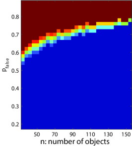
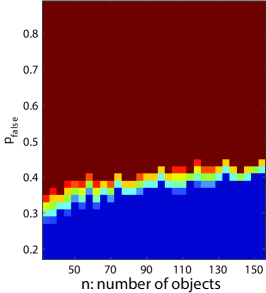
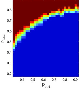
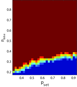
We follow the randomized model described in Section LABEL:sec:Theoretic-Guarantees to generate synthetic examples. For simplicity, we only consider the full observation mode, which establishes input maps between all pairs of objects. In all examples, we fix the universe size such that it consists of points. We then vary the remaining parameters, i.e., , and , to assess the performance of an algorithm. We evaluate sets of parameters for each scenario, where each parameter configuration is simulated by 10 Monte Carlo trials. The empirical success probability is reflected by the color of each cell. Blue denotes perfect recovery in all experiments, and red denotes failure for all trials.
 |
 |
| (a) | (b) |
 |
 |
| (c) | (d) |
labelFig:PT
Figure LABEL:Fig:PT(a) illustrates the phase transition for , when the number of objects and vary. We can see that MatchLift is exact even when the majority of the input correspondences are incorrect (e.g., when ). This is consistent with the theoretical result that the lower bound on for exact recovery is .
Figure LABEL:Fig:PT(c) shows the phase transition for , when and vary. We can see that MatchLift tolerates more noise when is large. This is also consistent with the result that the error-correction ability improves with .
5.2 Real-World Examples
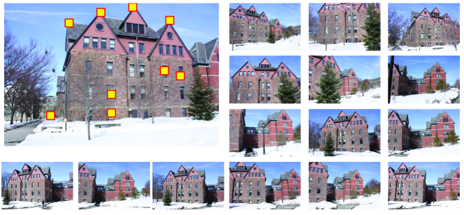
labelFig:Benchmark-building
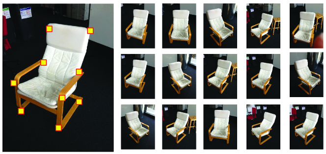
labelFig:Benchmark-chair
We have applied our algorithm on six benchmark datasets, i.e., CMU-House, CMU-Hotel, two datasets (Graf and Bikes) from [39]111available online: robots.ox.ac.uk/ vgg/research/affine and two new datasets (referred as Chair and Building, respectively) designed for evaluating joint partial object matching. As shown in Figures LABEL:Fig:Benchmark-building and LABEL:Fig:Benchmark-chair, the Building data set contains images taken around a building [4], while the Chair data set contains images of a chair model from different viewpoints. In the following, we first discuss the procedure for generating the input to our algorithm, i.e., the input sets and the initial maps. We then present the evaluation setup and analyze the results.
-
•
Feature points and initial maps. To make fair comparisons with previous techniques on CMU-House and CMU-Hotel, we use the features points provided in [15] and apply the spectral matching algorithm described in [40] to establish initial maps between features points. To assess the performance of the proposed algorithm with sparse input maps, we only match each image with random neighboring images.
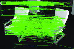
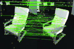
(a) (b) Figure 4: A map between dense SIFT feature points (a) is converted into a map between sampled feature points (b. labelFig:Downsampling
-
•
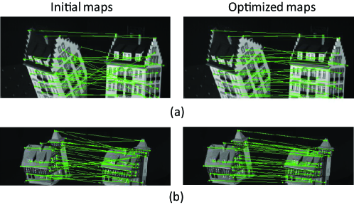
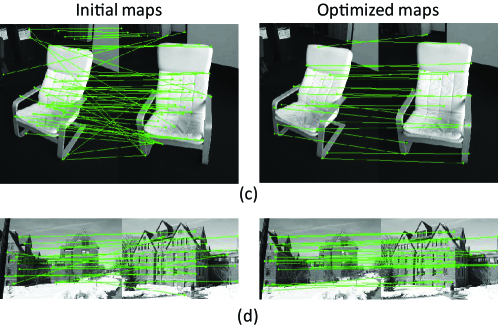
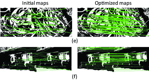
Figure 5: Comparisons between the input maps and the output of MatchLift on six benchmark datasets: (a) CMU Hotel, (b) CMU House, (c) Chair, (d) Building, (e) Graf, and (f) Bikes. The optimized maps not correct incorrect correspondences as well as fill in missing correspondences (generated by paths through intermediate shapes). One representative pair from each dataset is shown here. labelFig:Comparison-CMU
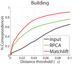
To handle raw images in Chair, Building, Graf and Bikes, we apply a different strategy to build feature points and initial maps. We first detect dense SIFT feature points [41] on each image. We then apply RANSAC [42] to obtain correspondences between each pair of images. As SIFT feature points are over-complete, many of them do not appear in the resulting feature correspondences between pairs of views. Thus, we remove all feature points that have less than appearances in all pair-wise maps. We further apply farthest point sampling on the feature points until the sampling density is above , where is the width of the input images. The remaining feature points turn out to be much more distinct and thus are suitable for joint matching (See Figure LABEL:Fig:Downsampling). For the experiments we have tested, we obtain about features points per image.
-
•
Evaluation protocol. On CMU-House and CMU-Hotel, we count the percentage of correct feature correspondences produced by each algorithm. On Chair, Building, Graf and Bikes, we apply the metric described in [43], which evaluates the deviations of manual feature correspondences. As the feature points computed on each image do not necessarily align with the manual features, we apply [44] to interpolate feature level correspondences into pixel-wise correspondences for evaluation.
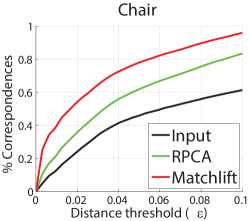
(a) (b) 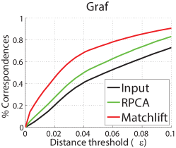
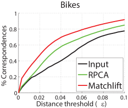
(c) (d) Figure 6: Percentages of ground-truth correspondences, whose distances to a map collection are below a varying threshold . labelFig:Benchmark1
Input MatchLift RPCA LearnI LearnII House 68.2% 100% 92.2% 99.8% 96% Hotel 64.1% 100% 90.1% 99.8% 90% Table 2: Matching performance on the hotel and house datasets. We compare the proposed MatchLift algorithm with Robust PCA (RPCA) and two learning based graph matching methods: LearnI [45] and LearnII [15]. labelTable:CMU
-
•
Results. Table LABEL:Table:CMU shows the results of various algorithms on CMU-House and CMU-Hotel. We can see that even with moderate initial maps, MatchLift recovers all ground-truth correspondences. In contrast, the method of [29] can only recover and ground-truth correspondences on CMU-House and CMU-Hotel, respectively. Note that, MatchLift also outperforms state-of-the-art learning based graph matching algorithms [15, 45]. This shows the the advantage of joint object matching.
Figure LABEL:Fig:Comparison-CMU and Figure LABEL:Fig:Benchmark1 illustrate the results of MatchLift on Chair, Building, Graf and Bikes. As these images contain noisy background information, the quality of the input maps is lower than those on House and Hotel. Encouragingly, MatchLift still recovers almost all manual correspondences. Moreover, MatchLift significantly outperforms [29], as the fault-tolerance rate of [29] is limited by a small constant barrier.
Another interesting observation is that the improvements on Graf and Bikes (each has 6 images) are lower than those on Chair and Building (each has 16 images). This is consistent with the common knowledge of data-driven effect, where large object collections possess stronger self-correction power than small object collections.
6 Conclusionslabelsec:Conclusions
This paper delivers some encouraging news: given a few noisy object matches computed in isolation, a collection of partially similar objects can be accurately matched via semidefinite relaxation – an approach which provably works under dense errors. The proposed algorithm is essentially parameter-free, and can be solved by ADMM achieving remarkable efficiency and accuracy, with the assistance of a greedy rounding strategy.
The proposed algorithm achieves near-optimal error-correction ability, as it is guaranteed to work even when a dominant fraction of inputs are corrupted. This in turn underscore the importance of joint object matching: however low the quality of input sources is, perfect matching is achievable as long as we obtain sufficiently many instances. Also, while partial matching may incur much more severe input errors than those occurring in full-similarity matching, in many situations, the recovery ability of our algorithm is nearly the same as that in the full-similarity case (up to some constant factor). In a broader sense, our findings suggest that a large class of combinatorial / integer programming problems might be solved perfectly by semidefinite relaxation.
Appendix A Alternating Direction Method of Multipliers (ADMM)labelsec:ADMM-Appendix
This section presents the procedure for the ADMM algorithm. For notational simplicity, we represent the convex program as follows:
| dual variable | ||||
| subject to | ||||
where we denote . The matrices and operators are defined as follows
(i) encapsulate all block coefficient matrices for all ;
(ii) represents the constraint that () and the constraint ;
(iii) The variables on the right hand, i.e., and , represent dual variables associated with respective constraints.
The Lagrangian associated with the convex program can be given as follows
where denotes the conjugate operator w.r.t. an operator . The augmented Lagrangian for the convex program can now be written as
Here, the linear terms above represent the negative standard Lagrangian, whereas the quadratic parts represent the augmenting terms. is the penalty parameter that balances the standard Lagrangian and the augmenting terms. The ADMM then proceeds by alternately optimizing each primal and dual variable with others fixed, which results in closed-form solution for each subproblem. Denote by superscript the iteration number, then we can present the ADMM iterative update procedures as follows
| (17) | ||||
| (18) | ||||
| (19) |
Here, the operator (resp. ) denotes the projection onto the positive (resp. negative) semidefinite cone, and operator projects all entries of a vector / matrix to non-negative values. Within a reasonable amount of time, ADMM typically returns moderately acceptable results.
Appendix B Proof of Theorem LABEL:thm:SpectralMethodlabelsec:Proof_thm:SpectralMethod-m
The key step to the proof of Theorem LABEL:thm:SpectralMethod is to show that the set of outliers, even when they account for a dominant portion of the input matrix, behave only as a small perturbation to the spectrum of the non-corrupted components. Under the randomized model described in Section LABEL:sub:Randomized-Model, it can be easily seen that the trimming procedure is not invoked with high probability. Consequently, Theorem LABEL:thm:SpectralMethod can be established through the following lemma.
Lemma 1.
labellemma:SpectralMethod-mGiven any set of permutation matrices (), generate a random matrix via the following procedure.
-
1.
Generate a symmetric block matrix such that
and for all ,
(20) where and are independent binary variables, and are independent random permutation matrices obeying .
-
2.
is a principal minor of from rows / columns at indices from a set , where each is contained in independently with probability .
Then there exist absolute constants such that if , one has
| (21) |
with probability exceeding . Here, represents the th largest eigenvalue of .
Proof of Lemma LABEL:lemma:SpectralMethod-m.
Without loss of generality, we assume that for all , since rearranging rows / columns of does not change its eigenvalues. For convenience of presentation, we write such that
and for all :
| (22) |
This means that
| (23) |
Apparently, is a block diagonal matrix satisfying
| (24) |
which is only a mild perturbation of . This way we have reduced to the case where all blocks (including diagonal blocks) are i.i.d., which is slightly more convenient to analyze.
Decompose into 2 components such that
| (25) |
| (26) |
and
| (27) |
In other words, represents the mean component of , while comprises all variations around the mean component. It is straightforward to check that
If we denote by the principal minor coming from the rows and columns of at indices from , then from Weyl’s inequality one can easily see that
| (28) |
and
| (29) |
In light of this, it suffices to evaluate as well as the eigenvalues of .
We are now in position to quantify the eigenvalues of . Without affecting its eigenvalue distribution, one can rearrange the rows / columns of so that
| (30) |
Here, () denotes the cardinality of a set generated by independently sampling elements each with probability , and we set for simplicity. From Bernstein inequality, there exist universal constants such that if , then
| (31) |
holds with probability exceeding .
Since is positive semidefinite, from (LABEL:eq:Ymean_rearrange) one can easily check that all non-zero eigenvalues of are also eigenvalues of the following matrix
| (44) | ||||
| (50) | ||||
| (59) |
where
and
which satisfies .
By Schur complement condition for positive definite matrices [46], if , then and . Applying this condition to suggests that can only hold when
which however cannot be satisfied since . Thus, is rank deficient.
In fact, all non-zero eigenvalues of can be quantified as well. Specifically, for any vector
one can compute
| (60) |
That said, is an eigenvalue of with multiplicity . On the other hand, we have
| (61) |
indicating that is another eigenvalue of . Putting these together yields
| (62) |
Furthermore, the residual component can be bounded as follows
where the last inequality follows from (LABEL:eq:Concentration-ni). This taken collectively with (LABEL:eq:Yi_mean_decomposition) and (LABEL:eq:evalue_Yi0) yields that: when or, equivalently, when , one has
| (63) |
Furthermore, observe that , , and . When , Lemma LABEL:lemma:MomentMethod yields that
| (64) |
with probability at least . Hence, if for some constant .
Finally, the claim follows by substituting (LABEL:eq:EvalueYiMeanBound) and (LABEL:eq:Yvar_UB) into (LABEL:eq:Evalue-M-LB) and (LABEL:eq:Evalue-M-UB).∎
Appendix C Proof of Theorem LABEL:thm:RandomGraph-1 labelsec:Proof-of-Theorem-RandomGraph
To prove Theorem LABEL:thm:RandomGraph-1, we first analyze the Karush–Kuhn–Tucker (KKT) condition for exact recovery, which provides a sufficient and almost necessary condition for uniqueness and optimality. Valid dual certificates are then constructed to guarantee exact recovery.
C.1 Preliminaries and Notationslabelsec:Prelim
Without loss of generality, we can treat as a sub-matrix of an augmented square matrix such that
| (65) |
and
| (66) |
where the matrices are defined such that denotes the submatrix of coming from its rows at indices from . For instance, if , then one has
With this notation, represents a submatrix of coming from the rows at indices from and columns at indices from . Conversely, for any matrix , the matrix converts to an matrix space via zero padding.
With this notation, we can represent as a submatrix of , which is a corrupted version of and obeys
| (67) |
For notational simplicity, we set
| (68) |
Before continuing to the proof, it is convenient to introduce some notations that will be used throughout. Denote by and the support of and its complement support, respectively, and let and represent the orthogonal projection onto the linear space of matrices supported on and its complement support , respectively. Define to be the tangent space at w.r.t. all symmetric matrices of rank at most , i.e. the space of symmetric matrices of the form
| (69) |
and denote by its orthogonal complement. We then denote by (resp. ) the orthogonal projection onto (resp. ). In passing, if we define
| (70) |
then the columns of
| (71) |
form the set of eigenvectors of , and for any symmetric matrix ,
| (72) |
Furthermore, we define a vector to be
| (73) |
Put another way, if any row index of is associated with the element , then . One can then easily verify that
| (74) |
In fact, when ’s are sufficiently close to each other, is a good approximation of , as claimed in the following lemma.
Lemma 2.
labellemma:MeanApproxConsider a set of Bernoulli random variables (), and set . Let () be independent copies of , and denote . If , then the matrix
| (75) |
satisfies
| (76) |
and
| (77) |
with probability exceeding , where are some universal constants.
Proof.
See Appendix LABEL:sec:Proof_lemma:SpectralGapTight-1.∎
Since is equivalent to defined in (LABEL:eq:DefnA) up to row / column permutation, Lemma LABEL:lemma:MeanApprox reveals that
with high probability.
The following bound on the operator norm of a random block matrix is useful for deriving our main results.
Lemma 3.
labellemma:MomentMethodLet be a symmetric block matrix, where ’s are jointly independent matrices satisfying
| (78) |
Besides, holds for all . Then there exists an absolute constant such that
holds with probability exceeding .
Proof.
See Appendix LABEL:sec:Proof_lemma:MomentMethod.∎
Additionally, the second smallest eigenvalue of the Laplacian matrix of a random Erdős–Rényi graph can be bounded below by the following lemma.
Lemma 4.
labellemma:SpectralGapTightConsider an Erdős–Rényi graph and any positive integer , and let represent its (unnormalized) Laplacian matrix. There exist absolute constants such that if , then the algebraic connectivity of (i.e. the second smallest eigenvalue of ) satisfies
| (79) |
with probability exceeding .
Proof.
See Appendix LABEL:sec:Proof_lemma:SpectralGapTight.∎
Finally, if we denote by (resp. ) the number of sets () containing the element (resp. containing and simultaneously), then these quantities sharply concentrate around their mean values, as stated in the following lemma.
Lemma 5.
labellemma:ConcentrationThere are some universal constants such that if , then
hold with probability exceeding .
Proof.
In passing, the claim follows immediately from the Bernstein inequality that
where are i.i.d. random variables. Interested readers are referred to [47] for a tutorial.∎
C.2 Optimality and Uniqueness Conditionlabelsec:Duality
Recall that denotes the number of sets containing the element . The convex relaxation is exact if one can construct valid dual certificates, as summarized in the following lemma.
Lemma 6.
labellemma:KKTSuppose that there exist dual certificates , and obeying
| (80) | ||||
| (81) | ||||
| (82) | ||||
| (83) |
Then is the unique solution to MatchLift if either of the following two conditions is satisfied:
i) All entries of () within the support are strictly positive;
ii) For all satisfying ,
| (84) |
and, additionally,
| (85) |
Proof.
See Appendix LABEL:sec:Proof_lemma:KKT.∎
That said, to prove Theorem LABEL:thm:RandomGraph-1, it is sufficient (under the hypotheses of Theorem LABEL:thm:RandomGraph-1) to generate, with high probability, valid dual certificates , and obeying the optimality conditions of Lemma LABEL:lemma:KKT. This is the objective of the next subsection.
C.3 Construction of Dual Certificateslabelsec:DualConstruction
Decompose the input into two components , where
| (86) |
That said, (resp. ) consists of all correct (resp. incorrect) correspondences (i.e. non-zero entries) encoded in . This allows us to write
| (87) |
where and are defined to be
| (88) |
We propose constructing the dual certificate by producing three symmetric matrix components , , and separately, as follows.
-
1.
Construction of and . For any , define to be
(89) By setting , we produce and as follows
(90) and
(91) for some sufficiently large constant .
-
2.
Construction of and . We set
and
-
3.
Construction of and via an iterative procedure. Next, we generate via the following iterative procedure. Here, for any matrix , we let represent the entry in the block that encodes the correspondence from to .
Construction of a dual certificate . 1. initialize: Set the symmetric matrix such that and start with . 2. for each non-zero entry : 3. Set , and . 4. for each set : perform 5. output: . -
4.
Construction of and : define and such that
(92) (93)
Remark 5.
Below is a toy example to illustrate the proposed procedure for constructing . Consider three sets , , , and . Suppose that only contains two non-zero entries that incorrectly maps elements to in , as illustrated in Fig. LABEL:fig:BadPointExample(a). The resulting is shown in Fig. LABEL:fig:BadPointExample(b). Clearly, obeys .
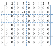 |
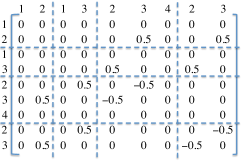 |
| (a) Input | (b) |
With the above construction procedure, one can easily verify that:
(1) , and are all contained in the space ;
(2) ;
(3) If we set , then for any ,
| (94) |
Furthermore, from Lemma LABEL:lemma:MeanApprox one can obtain
This taken collectively with (LABEL:eq:DefnMm) and the assumption (LABEL:eq:Lambda_Range) ensures that
| (95) |
as long as for some constant .
Consequently, we will establish that and are valid dual certificates if they satisfy
| (96) |
Such conditions will be established through the following lemmas.
Lemma 7.
labellemma:BoundYl_ZlThere are some universal constants such that
and
with probability exceeding .
Proof.
See Appendix LABEL:sec:Proof_lemma:BoundYl_Zl.∎
Lemma 8.
labellemma:BoundYtrueThere are some universal constants such that if and , then with probability exceeding , one has
and
for all unit vector satisfying .
Proof.
See Appendix LABEL:sec:Proof_lemma:BoundYtrue.∎
Combining Lemmas LABEL:lemma:BoundYl_Zl and LABEL:lemma:BoundYtrue yields that there exists an absolute constant such that if
then
On the other hand, observe that all entries of the non-negative matrix lying in the index set are bounded below in magnitude by . For sufficiently large , one can conclude that all entries of outside are strictly positive.
So far we have justified that and satisfy (LABEL:eq:RemainingCondition), thereby certifying that the proposed algorithm correctly recovers the ground-truth matching.
Appendix D Proofs of Auxiliary Lemmaslabelsec:ProofAuxiliaryLemmas
D.1 Proof of Lemma LABEL:lemma:MeanApproxlabelsec:Proof_lemma:SpectralGapTight-1
Denote by . From Bernstein inequality, sharply concentrates around such that if
| (97) |
with probability exceeding , where are some absolute constants.
The bound (LABEL:eq:ni_np_gap) also implies that
Similarly, one has
with probability exceeding , which implies that
Rewrite as
This allows us to bound the deviation of from as follows
for some universal constant .
On the other hand, it follows immediately from (LABEL:eq:ni_np_gap) that
for some absolute constant .
D.2 Proof of Lemma LABEL:lemma:MomentMethodlabelsec:Proof_lemma:MomentMethod
The norm of can be bounded via the moment method, which attempts to control for some even integer . See [48, Section 2.3.4] for a nice introduction.
Specifically, observe that can be expanded as follows
a trace sum over all -cycles in the vertex set . Note that are also treated as valid edges. For each term , if there exists an edge occurring exactly once, then the term vanishes due to the independence assumption. Thus, it suffices to examine the terms in which each edge is repeated at least twice. Consequently, there are at most relevant edges, which span at most distinct vertices. We also need to assign vertices to edges, which adds up to no more than different choices.
By following the same procedure and notation as adopted in [48, Page 119], we divide all non-vanishing -cycles into classes based on the above labeling order; each class is associated with () edges with multiplicities , where determines the class of cycles and . Since there are at most distinct vertices, one can see that no more than cycles falling within this particular class. For notational simplicity, set , and hence . By assumption (LABEL:eq:M_block_assumption), one has
Thus, the total contribution of this class does not exceed
By summing over all classes one obtains the crude bound
which follows that
If we set , then from Markov’s inequality we have
Since , there exists a constant such that
which completes the proof.
D.3 Proof of Lemma LABEL:lemma:SpectralGapTightlabelsec:Proof_lemma:SpectralGapTight
When , the adjacency matrix consists of independent Bernoulli components (except for diagonal entries), each with mean and variance . Lemma LABEL:lemma:MomentMethod immediately implies that if , then
| (98) |
with probability at least . That said, there exists an absolute constant such that
| (99) |
with probability exceeding .
On the other hand, from Bernstein inequality, the degree of each vertex exceeds
| (100) |
with probability at least , where is some constant. When , is connected, and hence the least eigenvalue of is zero with the eigenvector . This taken collectively with (LABEL:eq:AdjMatrixGnp) and (LABEL:eq:DegreeMatrixGnp) suggests that when , one has
with high probability.
D.4 Proof of Lemma LABEL:lemma:KKTlabelsec:Proof_lemma:KKT
Suppose that is the solution to MatchLift for some perturbation . By Schur complement condition for positive definiteness, the feasibility constraint is equivalent to
which immediately yields
| (101) |
and
| (102) |
The above inequalities follow from the facts and .
From Assumption (LABEL:eq:Y-tangent-space), one can derive
| (103) |
This allows us to bound
| (104) | ||||
| (105) | ||||
| (106) |
where the first inequality follows from (LABEL:eq:PSD_dd_H), and the last equality follows from Assumption (LABEL:eq:S_construction).
In order to preclude the possibility that is the solution to MatchLift, we need to show that . From (LABEL:eq:InnerProductYH) it suffices to establish that
| (107) |
for any feasible . In fact, since and are both positive semidefinite, one must have
| (108) |
On the other hand, the constraints
taken together imply that
| (109) |
Putting (LABEL:eq:YdH_non-neg) and (LABEL:eq:ZH_non-neg) together gives
Comparing this with (LABEL:eq:ZH_positive_Y), we only need to establish either or .
i) Suppose first that all entries of () in the support are strictly positive. If the identity holds, then the strict positivity assumption of on as well as the constraint immediately leads to
Besides, the feasibility constraint requires that . If , then all non-zero entries of are negative, and hence
which follows since all entries of are strictly positive. This contradicts with (LABEL:eq:PSD_dd_H). Consequently, we must either have or . This together with (LABEL:eq:ZH_positive_Y) establishes the claim.
ii) Next, we prove the claim under Assumptions (LABEL:eq:S_psd_Null) and (LABEL:eq:IiIj_constraint-KKTlemma). In fact, Assumption (LABEL:eq:S_psd_Null) together with (LABEL:eq:PSD_Pnm_H) asserts that can only occur if . This necessarily leads to , as claimed by Lemma LABEL:lemma:PgtH_H.
Lemma 9.
labellemma:PgtH_HSuppose that is feasible for MatchLift, and assume that
| (110) |
If , then one has .
Proof.
See Appendix LABEL:sec:Proof_lemma:PgtH_H.∎
In summary, we can conclude that is the unique optimizer in both cases.
D.5 Proof of Lemma LABEL:lemma:BoundYl_Zllabelsec:Proof_lemma:BoundYl_Zl
First, we would like to bound the operator norm of . Since each random matrix is independently drawn with mean , it is straightforward to see that
By observing that is constructed as a linear transform of , one can also obtain
Thus, it suffices to examine the deviation of incurred by the uncertainty of .
Denote by the component of generated due to the block , which clearly satisfies
For each non-zero entry of , if it encodes an incorrect correspondence between elements and , then it will affect no more than entries in , where each of these entries are affected in magnitude by an amount at most . Recall that represents the number of sets () containing and simultaneously, which sharply concentrates within as asserted in Lemma LABEL:lemma:Concentration. As a result, the sum of squares of these affected entries is bounded by
| (111) |
Moreover, since each row / column of can have at most one non-zero entry, we can rearrange with row / column permutation such that becomes a block-diagonal matrix, where the components affected by different entries of are separated into distinct diagonal blocks. This together with (LABEL:eq:FroNorm_Aij) leads to
and hence
for some absolute constant , where the last inequality follows from Lemma LABEL:lemma:Concentration.
Observe that are independently generated with mean zero, whose operator norm is bounded above by . Applying the matrix Bernstein inequality [49, Theorem 1.4] suggests that there exist universal constants such that for any ,
Put in another way, there exists a universal constant such that
| (112) |
holds with probability exceeding . This follows from Lemma LABEL:lemma:Concentration.
Additionally, observe that and
as long as . Applying Lemma LABEL:lemma:MomentMethod suggests that
with probability at least . This combined with (LABEL:eq:A_bound) yields
with probability at least , where is some universal constant.
On the other hand, for each entry of (), it can only be affected by those observed blocks (or ) satisfying (or ). Consequently, each entry of can be expressed as a sum of zero-mean independent variables, each of them being bounded in magnitude by . From Hoeffding’s inequality one can derive
for some constants , indicating that
with probability exceeding .
D.6 Proof of Lemma LABEL:lemma:BoundYtruelabelsec:Proof_lemma:BoundYtrue
By construction of , one can see that all non-zero entries lie within the support . One important feature of is that it can be converted, via row / column permutation, into a block diagonal matrix that consists of all-one blocks, where the block is of size (). From Lemma LABEL:lemma:Concentration, one has
with high probability. Thus, can also be rearranged such that its non-zero entries form disjoint diagonal blocks. We will quantify the eigenvalues of by bounding the spectrum of each of these matrix blocks.
We first decompose the matrix into two parts and such that
and
That said, consists of all non-corrupted components, while consists of all “debiased” random outliers.
By Lemma LABEL:lemma:SpectralGapTight, one can verify that for all unit vector such that ,
| (113) |
for some absolute constant , where the second inequality follows from the concentration result stated in Lemma LABEL:lemma:Concentration.
In addition, each entry of () lying in the support has mean zero and variance . Lemma LABEL:lemma:MomentMethod then suggests that the norm of each non-zero block of (the ones with size ) is bounded above by . As a result,
This taken collectively with (LABEL:eq:BoundYtrue) yields that
| (114) |
On the other hand, we know from the construction procedure and Lemma LABEL:lemma:MeanApprox that
for some constants . Since , we can also rearrange into diagonal blocks each of size (). Hence, a crude upper bound yields
for some universal constant .
D.7 Proof of Lemma LABEL:lemma:PgtH_Hlabelsec:Proof_lemma:PgtH_H
Define an augmented matrix such that
| (115) |
Recall that denotes the number of sets containing element , and that
The assumption that can be translated into
We can easily compute that
where
This combined with the identity (and hence ) yields
Summing over all leads to
Expanding it yields
From our assumption that , we can derive
| (116) |
Due to the feasibility constraint, all diagonal entries of are non-positive, and all off-diagonal entries of are non-negative. These conditions together with (LABEL:eq:H_avg_zero) establish that .
References
- [1] T. S. Cho, S. Avidan, and W. T. Freeman, “A probabilistic image jigsaw puzzle solver,” in IEEE Conference on Computer Vision and Pattern Recognition (CVPR), 2010, pp. 183–190.
- [2] D. Goldberg, C. Malon, and M. Bern, “A global approach to automatic solution of jigsaw puzzles,” Comput. Geom. Theory Appl., vol. 28, pp. 165–174, June 2004.
- [3] C. Zach, M. Klopschitz, and M. Pollefeys, “Disambiguating visual relations using loop constraints,” in IEEE Conference on Computer Vision and Pattern Recognition (CVPR), 2010, pp. 1426–1433.
- [4] D. Crandall, A. Owens, N. Snavely, and D. Huttenlocher, “Discrete-continuous optimization for large-scale structure from motion,” in IEEE Conference on Computer Vision and Pattern Recognition (CVPR), 2011, pp. 3001–3008.
- [5] Q.-X. Huang, S. Flöry, N. Gelfand, M. Hofer, and H. Pottmann, “Reassembling fractured objects by geometric matching,” in ACM Transactions on Graphics (TOG), vol. 25, no. 3. ACM, 2006, pp. 569–578.
- [6] L. Zhu, Z. Zhou, and D. Hu, “Globally consistent reconstruction of ripped-up documents,” IEEE Transactions on Pattern Analysis and Machine Intelligence, vol. 30, no. 1, pp. 1–13, 2008.
- [7] W. Marande and G. Burger, “Mitochondrial DNA as a genomic jigsaw puzzle,” Science, vol. 318, no. 5849, pp. 415–415, 2007.
- [8] R. Roberts, S. N. Sinha, R. Szeliski, and D. Steedly, “Structure from motion for scenes with large duplicate structures,” in IEEE Conference on Computer Vision and Pattern Recognition (CVPR), 2011, pp. 3137–3144.
- [9] A. Nguyen, M. Ben-Chen, K. Welnicka, Y. Ye, and L. Guibas, “An optimization approach to improving collections of shape maps,” in Computer Graphics Forum, vol. 30, no. 5. Wiley Online Library, 2011, pp. 1481–1491.
- [10] Q. Huang, G. Zhang, L. Gao, S. Hu, A. Butscher, and L. Guibas, “An optimization approach for extracting and encoding consistent maps in a shape collection,” ACM Transactions on Graphics, vol. 31, no. 6, p. 167, 2012.
- [11] V. Kim, W. Li, N. Mitra, S. DiVerdi, and T. Funkhouser, “Exploring collections of 3d models using fuzzy correspondences,” in ACM SIGGRAPH, 2012.
- [12] Q. Huang and L. Guibas, “Consistent shape maps via semidefinite programming,” Computer Graphics Forum, vol. 32, no. 5, pp. 177–186, 2013.
- [13] C. Schellewald and C. Schnörr, “Probabilistic subgraph matching based on convex relaxation,” in Energy minimization methods in computer vision and pattern recognition. Springer, 2005, pp. 171–186.
- [14] T. Cour, P. Srinivasan, and J. Shi, “Balanced graph matching,” Advances in Neural Information Processing Systems (NIPS), 2007.
- [15] T. S. Caetano, J. J. McAuley, L. Cheng, Q. V. Le, and A. J. Smola, “Learning graph matching,” IEEE Transactions on Pattern Analysis and Machine Intelligence, vol. 31, no. 6, pp. 1048–1058, 2009.
- [16] D. Pachauri, R. Kondor, and V. Singh, “Solving the multi-way matching problem by permutation synchronization.” in Advanced in Neural Information Processing Systems (NIPS), 2013.
- [17] L. Wang and A. Singer, “Exact and stable recovery of rotations for robust synchronization,” arxiv:1211.2441, 2013.
- [18] K. Chaudhury, Y. Khoo, A. Singer, and D. Cowburn, “Global registration of multiple point clouds using semidefinite programming,” arXiv:1306.5226, 2013.
- [19] E. J. Candes and B. Recht, “Exact matrix completion via convex optimization,” Foundations of Computational Mathematics, vol. 9, no. 6, pp. 717–772, April 2009.
- [20] R. H. Keshavan, A. Montanari, and S. Oh, “Matrix completion from a few entries,” IEEE Transactions on Information Theory, vol. 56, no. 6, pp. 2980–2998, 2010.
- [21] E. J. Candès, X. Li, Y. Ma, and J. Wright, “Robust principal component analysis?” Journal of ACM, vol. 58, no. 3, pp. 11:1–11:37, Jun 2011.
- [22] V. Chandrasekaran, S. Sanghavi, P. Parrilo, and A. S. Willsky, “Rank-sparsity incoherence for matrix decomposition,” SIAM Journal on Optimization, vol. 21, no. 2, 2011.
- [23] H. Xu, C. Caramanis, and S. Sanghavi, “Robust pca via outlier pursuit,” Advances on Neural Information Processing Systems (NIPS), 2010.
- [24] A. Ganesh, J. Wright, X. Li, E. J. Candes, and Y. Ma, “Dense error correction for low-rank matrices via principal component pursuit,” in IEEE International Symposium on Information Theory Proceedings (ISIT), 2010, pp. 1513–1517.
- [25] Y. Chen, A. Jalali, S. Sanghavi, and C. Caramanis, “Low-rank matrix recovery from errors and erasures,” IEEE Transactions on Information Theory, vol. 59, no. 7, pp. 4324–4337, July 2013.
- [26] J. Xu, R. Wu, K. Zhu, B. Hajek, R. Srikant, and L. Ying, “Jointly clustering rows and columns of binary matrices: Algorithms and trade-offs,” arxiv:1310.0512, 2013.
- [27] N. Bansal, A. Blum, and S. Chawla, “Correlation clustering,” Machine Learning, vol. 56, no. 1-3, pp. 89–113, 2004.
- [28] C. Mathieu and W. Schudy, “Correlation clustering with noisy input,” in ACM-SIAM SODA, 2010, pp. 712–728.
- [29] A. Jalali, Y. Chen, S. Sanghavi, and H. Xu, “Clustering partially observed graphs via convex optimization,” International Conf. on Machine Learning (ICML), 2011.
- [30] Y. Chen, S. Sanghavi, and H. Xu, “Clustering sparse graphs,” Advances in Neural Information Processing Systems (NIPS), 2012.
- [31] A. Jalali and N. Srebro, “Clustering using max-norm constrained optimization,” International Conference on Machine Learning (ICML), June 2012.
- [32] N. Ailon, Y. Chen, and X. Huan, “Breaking the small cluster barrier of graph clustering,” International Conference on Machine Learning (2013), 2013.
- [33] R. H. Keshavan, A. Montanari, and S. Oh, “Matrix completion from noisy entries,” Journal of Machine Learning Research, vol. 99, pp. 2057–2078, 2010.
- [34] J. L. Horner and P. D. Gianino, “Phase-only matched filtering,” Applied optics, vol. 23, no. 6, pp. 812–816, 1984.
- [35] A. Singer, “Angular synchronization by eigenvectors and semidefinite programming,” Applied and computational harmonic analysis, vol. 30, no. 1, pp. 20–36, 2011.
- [36] A. S. Bandeira, M. Charikar, A. Singer, and A. Zhu, “Multireference alignment using semidefinite programming,” in Conference on Innovations in Theoretical Computer Science, 2014, pp. 459–470.
- [37] Z. Wen, D. Goldfarb, and W. Yin, “Alternating direction augmented lagrangian methods for semidefinite programming,” Mathematical Programming Computation, vol. 2, no. 3-4, pp. 203–230, 2010.
- [38] R. Durrett, Random graph dynamics. Cambridge university press, 2007, vol. 20.
- [39] K. Mikolajczyk and C. Schmid, “A performance evaluation of local descriptors,” IEEE Transactions on Pattern Analysis and Machine Intelligence, vol. 27, no. 10, pp. 1615–1630, 2005.
- [40] M. Leordeanu and M. Hebert, “A spectral technique for correspondence problems using pairwise constraints,” in IEEE International Conference on Computer Vision (ICCV), vol. 2, 2005, pp. 1482–1489.
- [41] D. G. Lowe, “Distinctive image features from scale-invariant keypoints,” International journal of computer vision, vol. 60, no. 2, pp. 91–110, 2004.
- [42] M. A. Fischler and R. C. Bolles, “Random sample consensus: a paradigm for model fitting with applications to image analysis and automated cartography,” Commun. ACM, vol. 24, no. 6, pp. 381–395, Jun. 1981.
- [43] Y. HaCohen, E. Shechtman, D. Goldman, and D. Lischinski, “Non-rigid dense correspondence with applications for image enhancement,” ACM Trans. Graph., vol. 30, no. 4, pp. 70:1–70:10, Jul. 2011.
- [44] N. Ahmed, C. Theobalt, C. Rossl, S. Thrun, and H. Seidel, “Dense correspondence finding for parametrization-free animation reconstruction from video.” in CVPR, 2008.
- [45] M. Leordeanu, R. Sukthankar, and M. Hebert, “Unsupervised learning for graph matching,” International journal of computer vision, vol. 96, no. 1, pp. 28–45, 2012.
- [46] S. P. Boyd and L. Vandenberghe, Convex optimization. Cambridge university press, 2004.
- [47] N. Alon and J. H. Spencer, The probabilistic method (3rd Edition). Wiley, 2008.
- [48] T. Tao, Topics in random matrix theory. AMS Bookstore, 2012, vol. 132.
- [49] J. A. Tropp, “User-friendly tail bounds for sums of random matrices,” Foundations of Computational Mathematics, vol. 12, no. 4, pp. 389–434, 2012.