Adaptive ABC model choice and geometric summary statistics for hidden Gibbs random fields

Abstract

Selecting between different dependency structures of hidden Markov random field can be very challenging, due to the intractable normalizing constant in the likelihood. We answer this question with approximate Bayesian computation (ABC) which provides a model choice method in the Bayesian paradigm. This comes after the work of Grelaud et al. (2009) who exhibited sufficient statistics on directly observed Gibbs random fields. But when the random field is latent, the sufficiency falls and we complement the set with geometric summary statistics. The general approach to construct these intuitive statistics relies on a clustering analysis of the sites based on the observed colors and plausible latent graphs. The efficiency of ABC model choice based on these statistics is evaluated via a local error rate which may be of independent interest. As a byproduct we derived an ABC algorithm that adapts the dimension of the summary statistics to the dataset without distorting the model selection.

Keywords: Approximate Bayesian Computation, model choice, hidden Gibbs random fields, summary statistics, misclassification rate, $k$-nearest neighbors

1 Introduction

Gibbs random fields are polymorphous statistical models, that are useful to analyse different types of spatially correlated data, with a wide range of applications, including image analysis (Hurn et al., 2003), disease mapping (Green and Richardson, 2002), genetic analysis (François et al., 2006) among others. The autobinomial model (Besag, 1974) which encompasses the Potts model, is used to describe the spatial dependency of discrete random variables (e.g., shades of grey or colors) on the vertices of an undirected graph (e.g., a regular grid of pixels). See for example Alfò et al. (2008) and Moores, Hargrave, Harden, and Mengersen (2014) who performed image segmentation with the help of the above modeling. Despite their popularity, these models present major difficulties from the point of view of either parameter estimation (Friel et al., 2009, Friel, 2012, Everitt, 2012) or model choice (Grelaud et al., 2009, Friel, 2013, Cucala and Marin, 2013), due to an intractable normalizing constant. Remark the exception of small latices on which we can apply the recursive algorithm of Reeves and Pettitt (2004), Friel and Rue (2007) and obtain a reliable approximation of the normalizing constant. However, the complexity in time of the above algorithm grows exponentially and is thus helpless on large lattices.

The present paper deals with the challenging problem of selecting a dependency structure of an hidden Potts model in the Bayesian paradigm and explores the opportunity of approximate Bayesian computation (ABC, Tavaré et al., 1997, Pritchard et al., 1999, Marin et al., 2012, Baragatti and Pudlo, 2014) to answer the question. Up to our knowledge, this important question has not yet been addressed in the Bayesian literature. Alternatively we could have tried to set up a reversible jump Markov chain Monte Carlo, but follows an important work for the statistician to adapt the general scheme, as shown by Caimo and Friel (2011, 2013) in the context of exponential random graph models where the observed data is a graph. Cucala and Marin (2013) addressed the question of inferring the number of latent colors with an ICL criterion but their complex algorithm cannot be extended easily to choose the dependency structure. Other approximate methods have also been tackled in the literature such as pseudo-likelihoods (Besag, 1975), mean field approximations (Forbes and Peyrard, 2003) but lacks theoretical support.

Approximate Bayesian computation (ABC) is a simulation based approach that can addresses the model choice issue in the Bayesian paradigm. The algorithm compares the observed data $y^{\text{obs}}$ with numerous simulations $y$ through summary statistics $S(y)$ in order to supply a Monte Carlo approximation of the posterior probabilities of each model. The choice of such summary statistics presents major difficulties that have been especially highlighted for model choice (Robert et al., 2011, Didelot et al., 2011). Beyond the seldom situations where sufficient statistics exist and are explicitly known (Gibbs random fields are surprising examples, see Grelaud et al., 2009), Marin et al. (2013) provide conditions which ensure the consistency of ABC model choice. The present work has thus to answer the absence of available sufficient statistics for hidden Potts fields as well as the difficulty (if not the impossibility) to check the above theoretical conditions in practice.

Recent articles have proposed automatic schemes to construct theses statistics (rarely from scratch but based on a large set of candidates) for Bayesian parameter inference and are meticulously reviewed by Blum et al. (2013) who compare their performances in concrete examples. But very few has been accomplished in the context of ABC model choice apart from the work of Prangle et al. (2013). The statistics $S(y)$ reconstructed by Prangle et al. (2013) have good theoritical properties (those are the posterior probabilities of the models in competition) but are poorly approximated with a pilot ABC run (Robert et al., 2011), which is also time consuming.

The paper is organized as follows: Section 2 presents ABC model choice as a $k$-nearest neighbor classifier, and defines a local error rate which is the first contribution of the paper. We also provide an adaptive ABC algorithm based on the local error to select automatically the dimension of the summary statistics. The second contribution is the introduction of a general and intuitive approach to produce geometric summary statistics for hidden Potts model in Section 3. We end the paper with numerical results in that framework.

2 Local error rates and adpative ABC model choice

When dealing with models whose likelihood cannot be computed analytically, Bayesian model choice becomes challenging since the evidence of each model writes as the integral of the likelihood over the prior distribution of the model parameter. ABC provides a method to escape from the intractability problem and relies on many simulated datasets from each model either to learn the model that fits the observed data $y^{\text{obs}}$ or to approximate the posterior probabilities. We refer the reader to reviews on ABC (Marin et al., 2012, Baragatti and Pudlo, 2014) to get a wider presentation and will focus here on the model choice procedure.

2.1 Background on Approximate Bayesian computation for model choice

Assume we are given $M$ stochastic models with respective paramater spaces embedded into Euclidean spaces of various dimensions. The joint Bayesian distribution sets

• a prior on the model space, $\pi(1),\ldots,\pi(M)$,

• for each model, a prior on its parameter space, whose density with respect to a reference measure (often the Lebesgue measure of the Euclidean space) is $\pi_{m}(\theta_{m})$ and

• the likelihood of the data $y$ within each model, namely $f_{m}(y|\theta_{m})$.

The evidence of model $m$ is then defined as

$$e(m,y):=\int f_{m}(y|\theta_{m})\pi_{m}(\theta_{m})\mathrm{d}\theta_{m}$$

and the posterior probability of model $m$ as

$$\pi(m|y)=\frac{\pi(m)e(m,y)}{\sum_{m^{\prime}}\pi(m^{\prime})e(m^{\prime},y)}.$$ (1)

When the goal of the Bayesian analysis is the selection of the model that best fits the observed data $y^{\text{obs}}$, it is performed through the maximum a posteriori (MAP) defined by

$$\widehat{m}_{\text{MAP}}(y^{\text{obs}})=\operatorname{arg\,max}_{m}\pi(m|y^{\text{obs}}).$$ (2)

The latter can be seen as a classification problem predicting the model number given the observation of $y$. From this standpoint, $\widehat{m}_{\text{MAP}}$ is the Bayes classifier, well known to minimize the 0-1 loss (Devroye et al., 1996). One might argue that $\widehat{m}_{\text{MAP}}$ is an estimator defined as the mode of the posterior probabilities which form the density of the posterior with respect to the counting measure. But the counting measure, namely $\delta_{1}+\cdots+\delta_{M}$, is a canonical reference measure, since it is invariant to any permutation of $\{1,\ldots,M\}$ whereas no such canonical reference measure (invariant to one-to-one transformation) exists on compact subset of the real line. Thus (2) does not suffer from the drawbacks of posterior mode estimators (Druilhet and Marin, 2007).

To approximate $\widehat{m}_{\text{MAP}}$, ABC starts by simulating numerous triplets $(m,\theta_{m},y)$ from the joint Bayesian model. Afterwards, the algorithm mimics the Bayes classifier (2): it approximates the posterior probabilities by the frequency of each model number associated with simulated $y$’s in a neighborhood of $y^{\text{obs}}$. If required, we can eventually predict the best model with the most frequent model in the neighborhood, or, in other words, take the final decision by plugging in (2) the approximations of the posterior probabilities.

If directly applied, this first, naive algorithm faces the curse of dimensionality, as simulated datasets $y$ can be complex objects and lie in a space of high dimension (e.g., numerical images). Indeed, finding a simulated dataset in the vicinity of $y^{\text{obs}}$ is almost impossible when the ambient dimension is high. The ABC algorithm performs therefore a (non linear) projection of the observed and simulated datasets onto some Euclidean space of reasonable dimension via a function $S$, composed of summary statistics. Moreover, due to obvious reasons regarding computer memory, instead of keeping track of the whole simulated datasets, one commonly saves only the simulated vectors of summary statistics, which leads to a table composed of iid replicates $(m,\theta_{m},S(y))$, often called the reference table in the ABC literature, see Algorithm 1.

Output: A reference table of size $n_{\text{REF}}$

for $j\leftarrow 1$ to $n_{\text{REF}}$ do

       draw $m$ from the prior $\pi$;

       draw $\theta$ from the prior $\pi_{m}$;

       draw $y$ from the likelihood $f_{m}(\cdot|\theta)$;

       compute $S(y)$;

       save $(m_{j},\theta_{j},S(y_{j}))\leftarrow(m,\theta,S(y))$;

      

end for

return the table of $(m_{j},\theta_{j},S(y_{j}))$, $j=1,\ldots,n_{\text{REF}}$

Algorithm 1 Simulation of the ABC reference table

From the standpoint of machine learning, the reference table serves as a training database composed of iid replicates drawn from the distribution of interest, namely the joint Bayesian model. The regression problem of estimating the posterior probabilities or the classification problem of predicting a model number are both solved with nonparametric methods. The neighborhood of $y^{\text{obs}}$ is thus defined as simulations whose distances to the observation measured in terms of summary statistics, i.e., $\rho(S(y),S(y^{\text{obs}}))$, fall below a threshold $\varepsilon$ commonly named the tolerance level. The calibration of $\varepsilon$ is delicate, but had been partly neglected in the papers dealing with ABC that first focused on decreasing the total number of simulations via the recourse to Markov chain Monte Carlo (Marjoram et al., 2003) or sequential Monte Carlo methods (Beaumont et al., 2009, Del Moral et al., 2012) whose common target is the joint Bayesian distribution conditioned by $\rho(S(y),S(y^{\text{obs}}))\leq\varepsilon$ for a given $\varepsilon$. By contrast, the simple setting we adopt here reveals the calibration question. In accepting the machine learning viewpoint, we can consider the ABC algorithm as a $k$-nearest neighbor (knn) method, see Biau et al. (2013); the calibration of $\varepsilon$ is thus transformed into the calibration of $k$. The Algorithm we have to calibrate is given in Algorithm 2.

Output: A sample of size $k$ distributed according to the ABC approximation of the posterior

simulate the reference table $\mathscr{T}$ according to Algorithm 1;

sort the replicates of $\mathscr{T}$ according to $\rho(S(y_{j}),S(y^{\text{obs}}))$;

keep the $k$ first replicates;

return the relative frequencies of each model among the $k$ first replicates and the most frequent model;

Algorithm 2 Uncalibrated ABC model choice

Before entering into the tuning of $k$, we highlight that the projection via the summary statistics generates a difference with the standard knn methods. Under mild conditions, knn are consistent nonparametric methods. Consequently, as the size of the reference table tends to infinity, the relative frequency of model $m$ returned by Algorithm 2 converges to

$$\pi(m|S(y^{\text{obs}})).$$

Unfortunately, when the summary statistics are not sufficient for the model choice problem, Didelot et al. (2011) and Robert et al. (2011) found that the above probability can greatly differ from the genuine $\pi(m|y^{\text{obs}})$. Afterwards Marin et al. (2013) provide necessary and sufficient conditions on $S(\cdot)$ for the consistency of the MAP based on $\pi(m|S(y^{\text{obs}}))$ when the information included in the dataset $y^{\text{obs}}$ increases, i.e. when the dimension of $y^{\text{obs}}$ tends to infinity. Consequently, the problem that ABC addresses with reliability is classification, and the mentioned theoretical results requires a shift from the approximation of posterior probabilities. Practically the frequencies returned by Algorithm 2 should solely be used to order the models with respect to their fits to $y^{\text{obs}}$ and construct a knn classifier $\widehat{m}$ that predicts the model number.

It becomes therefore obvious that the calibration of $k$ should be done by minimizing the misclassification error rate of the resulting classifier $\widehat{m}$. This indicator is the expected value of the 0-1 loss function, namely $\mathbf{1}\{\widehat{m}(y)\neq m\}$, over a random $(m,y)$ distributed according to the marginal (integrated in $\theta_{m}$) of the joint Bayesian distribution, whose density in $(m,y)$ writes

$$\pi(m)\int f_{m}(y|\theta_{m})\pi_{m}(\theta_{m})\mathrm{d}\theta_{m}.$$ (3)

Ingenious solutions have been already proposed and are now well established to fullfil this minimization goal and bypass the overfitting problem, based on cross-validation on the learning database. But, for the sake of clarity, particularly in the following sections, we decided to take advantage of the fact that ABC aims at learning on simulated databases, and we will use a validation reference table, simulated also with Algorithm 1, but independently of the training reference table, to evaluate the misclassification rate with the averaged number of differences between the true model numbers $m_{j}$ and the predicted values $\widehat{m}(y_{j})$ by knn (i.e. by ABC) on the validation reference table.

2.2 Local error rates

The misclassification rate $\tau$ of the knn classifier $\hat{m}$ at the core of Algorithm 2 provides consistant evidence of its global accuracy. It supplies indeed a well-known support to calibrate $k$ in Algorithm 2. The purpose of ABC model choice methods though is the analyse of an observed dataset $y^{\text{obs}}$ and this first indicator is irrelevant to assess the accuracy of the classifier at this precise point of the data space, since it is by nature a prior gauge. We propose here to disintegrate this indicator, and to rely on conditional expected value of the misclassification loss $\mathbf{1}\{\widehat{m}(y)\neq m\}$ knowing $y$ as an evaluation of the efficiency of the classifier at $y$. We recall the following proposition whose proof is easy, but might help clarifying matters when applied to the joint distribution (3).

Proposition 1.

Consider a classifier $\hat{m}$ that aims at predicting $m$ given $y$ on data drawn from the joint distribution $f(m,y)$. Let $\tau$ be the misclassification rate of $\hat{m}$, defined by $\mathbb{P}(\hat{m}(Y)\neq\mathscr{M})$, where $(\mathscr{M},Y)$ is a random pair with distribution $f$ under the probability measure $\mathbb{P}$. Then, (i) the expectation of the loss function is

$$\tau=\sum_{m}\int_{y}\mathbf{1}\{\widehat{m}(y)\neq m\}f(m,y)\,\mathrm{d}y.$$

Additionally, (ii), the conditional expectation knowing $y$, namely $\tau(y)=\mathbb{P}\big{(}\hat{m}(Y)\neq\mathscr{M}\big{|}Y=y\big{)}$, is

$$\tau(y)=\sum_{m}\mathbf{1}\{\widehat{m}(y)\neq m\}f(m|y)$$ (4)

and $\tau=\int_{y}f(y)\tau(y)\,\mathrm{d}y$, where $f(y)$ denotes the marginal distribution of $f$ (integrated over $m$) and $f(m|y)=f(m,y)/f(y)$ the conditional probability of $m$ given $y$. Furthermore, we have

$$\tau(y)=1-f(\widehat{m}(y)\,|\,y).$$ (5)

The last result (5) suggests that a conditional expected value of the misclassification loss is a valuable indicator of the error at $y$ since it is admitted that the posterior probability of the predicted model reveals the accuracy of the decision at $y$. Nevertheless, the whole simulated datasets are not saved into the ABC reference table but solely some numerical summaries $S(y)$ per simulated dataset $y$, as explained above. Thus the disintegration process of $\tau$ is practically limited to the conditional expectation of the loss knowing some non one-to-one function of $y$. Its definition becomes thereforemuch more subtle than the basic (4). Actually, the ABC classifier can be trained on a subset $S_{1}(y)$ of the summaries $S(y)$ saved in the training reference table, or on some deterministic function (we still write $S_{1}(y)$) of $S(y)$ that reduces the dimension, such as the projection on the LDA axes proposed by Estoup et al. (2012). To highlight this fact, the ABC classifier is denoted by $\widehat{m}(S_{1}(y))$ in what follows. It is worth noting here that the above setting encompasses any dimension reduction technique presented in the review of Blum et al. (2013), though the review in oriented on parameter inference. Furthermore we might want to disintegrate the misclassification rate with respect to another projection $S_{2}(y)$ of the simulated data that can or cannot be related to the summaries $S_{1}(y)$ used to train the ABC classifier, albeit $S_{2}(y)$ is also limited to be a deterministic function of $S(y)$. This yields the following.

Definition 2.

The local error rate of the $\widehat{m}(S_{1}(y))$ classifier with respect to $S_{2}(y)$ is

$$\tau_{S_{1}}(S_{2}(y)):=\mathbb{P}\big{(}\widehat{m}(S_{1}(Y))\neq\mathscr{M}\,\big{|}\,S_{2}(Y)=S_{2}(y)\big{)},$$

where $(\mathscr{M},Y)$ is a random variable with distribution given in (3).

The purpose of the local misclassification rate in the present paper is twofold and requires to play with the distinction between $S_{1}$ and $S_{2}$, as the last part will show on numerical examples. The first goal is the construction of a prospective tool that aims at checking whether a new statistic $S^{\prime}(y)$ carries additional information regarding the model choice, beyond a first set of statistics $S_{1}(y)$. In the latter case, it can be useful to localize the misclassification error of $\widehat{m}(S_{1}(y))$ with respect to the concatenated vector $S_{2}(y)=(S_{1}(y),S^{\prime}(y))$. Indeed, this local error rate can reveal concentrated areas of the data space, characterized in terms of $S_{2}(y)$, in which the local error rate rises above $(M-1)/M$, the averaged (local) amount of errors of the random classifier among $M$ models, so as to approach $1$. The interpretation of the phenomenon is as follows: errors committed by $\widehat{m}(S_{1}(y))$, that are mostly spread on the $S_{1}(y)$-space, might gather in particular areas of subspaces of the support of $S_{2}(y)=(S_{1}(y),S^{\prime}(y))$. This peculiarity is due to the dimension reduction of the summary statistics in ABC before the training of the classifier and represents a concrete proof of the difficulty of ABC model choice already raised by Didelot et al. (2011) and Robert et al. (2011).

The second goal of the local error rate given in Definition 2 is the evaluation of the confidence we may concede in the model predicted at $y^{\text{obs}}$ by $\widehat{m}(S_{1}(y))$, in which case we set $S_{2}(y)=S_{1}(y)$. And, when both sets of summaries agree, the results of Proposition 1 extend to

$$\tau_{S_{1}}(S_{1}(y)) =\sum_{m}\pi(m|S_{1}(y))\mathbf{1}\{\widehat{m}(S_{1}(y))=m\}$$

$$=1-\pi(\widehat{m}(S_{1}(y))\,|\,S_{1}(y)).$$ (6)

Besides the local error rate we propose in Definition 2 is an upper bound of the Bayes classifier if we admit the loss of information committed by replacing $y$ with the summaries.

Proposition 3.

Consider any classifier $\widehat{m}(S_{1}(y))$. The local error rate of this classifier satisfies

$$\tau_{S_{1}}(s_{2}) =\mathbb{P}\left(\widehat{m}(S_{1}(Y))\neq\mathscr{M}\,\middle|\,S_{2}(Y)=s_{2}\right)$$

$$\geq\mathbb{P}\left(\widehat{m}_{\text{\rm MAP}}(Y)\neq\mathscr{M}\,\middle|\,S_{2}(Y)=s_{2}\right),$$ (7)

where $\widehat{m}_{\text{\rm MAP}}$ is the Bayes classifier defined in (2) and $s_{2}$ any value in the support of $S_{2}(Y)$. Consequently,

$$\mathbb{P}\left(\widehat{m}(S_{1}(Y))\neq\mathscr{M}\right)\geq\mathbb{P}\left(\widehat{m}_{\text{\rm MAP}}(Y)\neq\mathscr{M}\right).$$ (8)

Proof.

Proposition 1, in particular (5), implies that $\widehat{m}_{\text{MAP}}(y)$ is the ideal classifier that minimizes the conditional $0$-$1$ loss knowing $y$. Hence, we have

$$\mathbb{P}\left(\widehat{m}(S_{1}(Y))\neq\mathscr{M}\,\middle|\,Y=y\right)\\ \geq\mathbb{P}\left(\widehat{m}_{\text{\rm MAP}}(Y)\neq\mathscr{M}\,\middle|\,Y=y\right).$$

Integrating the above with respect to the distribution of $Y$ knowing $S_{2}(Y)$ leads to (7), and a last integral to (8).∎

Proposition 3 shows that the introduction of new summary statistics cannot distort the model selection insofar as the risk of the resulting classifier cannot decrease below the risk of the Bayes classifier $\widehat{m}_{\text{MAP}}$. We give here a last flavor of the results of Marin et al. (2013) and mention that, if $S_{1}(y)=S_{2}(y)=S(y)$ and if the classifiers are perfect (i.e., trained on infinite reference tables), we can rephrase part of their results as providing mild conditions on $S$ under which the local error $\tau_{S}(S(y))$ tends to $0$ when the size of the dataset $y$ tends to infinity.

2.3 Estimation algorithm of the local error rates

The numerical estimation of the local error rate $\tau_{S_{1}}(S_{2}(y))$, as a surface depending on $S_{2}(y)$, is therefore paramount to assess the difficulty of the classification problem at any $s_{2}=S_{S}(y)$, and the local accuracy of the classifier. Naturally, when $S_{1}(y)=S_{2}(y)$ for all $y$, the local error can be evaluated at $S_{2}(y^{\text{obs}})$ by plugging in (6) the ABC estimates of the posterior probabilities (the relative frequencies of each model among the particles returned by Algorithm 2) as substitute for $\pi(m|S(y^{\text{obs}}))$. This estimation procedure is restricted to the above mentioned case where the set of statistics used to localize the error rate agrees with the set of statistics used to train the classifier. Moreover, the approximation of the posterior probabilities returned by Algorithm 2, i.e., a knn method, might not be trustworthy: the calibration of $k$ performed by minimizing the prior error rate $\tau$ does not provide any certainty on the estimated posterior probabilities beyond a ranking of these probabilities that yields the best classifier in terms of misclassification. In other words, the knn method calibrated to answer the classification problem of discriminating among models does not produce a reliable answer to the regression problem of estimating posterior probabilities. Certainly, the value of $k$ must be increased to face this second kind of issue, at the price of a larger bias that might even swap the model ranking (otherwise, the empirical prior error rate would not depend on $k$, see the numerical result section).

For all these reasons, we propose here an alternative estimate of the local error. The core idea of our proposal is the recourse to a nonparametric method to estimate conditional expected values based on the calls to the classifier $\widehat{m}$ on a validation reference table, already simulated to estimate the global error rate $\tau$. Nadaraya-Watson kernel estimators of the conditional expected values

$$\tau_{S_{1}}(S_{2}(y))=\\ \mathbb{E}\left(\mathbf{1}\{\widehat{m}(S_{1}(Y))\neq\mathscr{M}\}\,\middle|\,S_{2}(Y)=S_{2}(y)\right)$$ (9)

rely explicitly on the regularity of this indicator, as a function of $s_{2}=S_{2}(y)$, which contrasts with the ABC plug-in estimate described above. We thus hope improvements in the accuracy of error estimate and a more reliable approximation of the whole function $\tau_{S_{1}}(S_{2}(y))$. Additionally, we are not limited anymore to the special case where $S_{1}(y)=S_{2}(y)$ for all $y$. It is worth stressing here that the bandwidth of the kernels must be calibrated by minimizing the $L^{2}$-loss, since the target is a conditional expected value.

Input: A validation or test reference table and a classifier $\widehat{m}(S_{1}(y))$ fitted with a first reference table

Output: Estimations of (9) at each point of the second reference table

for each $(m_{j},y_{j})$ in the test table do

       compute $\delta_{j}=\{\widehat{m}(S_{1}(y_{j}))\neq m_{j}\}$;

      

end for

calibrate the bandwidth $\mathbf{h}$ of the Nadaraya-Watson estimator predicting $\delta_{j}$ knowing $S_{2}(y_{j})$ via cross-validation on the test table;

for each $(m_{j},y_{j})$ in the test table do

       evaluate the Nadaraya-Watson estimator with bandwidth $\mathbf{h}$ at $S_{2}(y_{j})$;

      

end for

Algorithm 3 Estimation of $\tau_{S_{1}}(S_{2}(y))$ given an classifier $\widehat{m}(S_{1}(y))$ on a validation or test reference table

Practically, this leads to Algorithm 3 which requires a validation or test reference table independent of the training database that constitutes the ABC reference table. We can bypass the requirement by resorting to cross validation methods, as for the computation of the global prior misclassification rate $\tau$. But the ensued algorithm is complex and it induces more calls to the classifier (consider, e.g,. a ten-fold cross validation algorithm computed on more than one random grouping of the reference table) than the basic Algorithm 3, whereas the training database can always be supplemented by a validation database since ABC, by its very nature, is a learning problem on simulated databases. Moreover, to display the whole surface $\tau_{S_{1}}(S_{2}(y))$, we can interpolate values of the local error between points $S_{2}(y)$ of the second reference table with the help of a Kriging algorithm. We performed numerical experiments (not detailed here) concluding that the resort to a Kriging algorithm provides results comparable to the evaluation of Nadaraya-Watson estimator at any point of the support of $S_{2}(y)$, and can reduce computation times.

2.4 Adaptive ABC

The local error rate can also represent a valuable way to adjust the summary statistics to the data point $y$ and to build an adaptive ABC algorithm achieving a local trade off that increases the dimension of the summary statistics at $y$ only when the additional coordinates add information regarding the classification problem. Assume that we have at our disposal a collection of ABC classifiers, $\widehat{m}_{\lambda}(y):=\widehat{m}_{\lambda}(S_{\lambda}(y))$, $\lambda=1,\ldots,\Lambda$, trained on various projections of $y$, namely the $S_{\lambda}(y)$’s, and that all these vectors, sorted with respect to their dimension, depend only on the summary statistics registered in the reference tables. Sometimes low dimensional statistics may suffice for the classification (of models) at $y$, whereas other times we may need to examine statistics of larger dimension. The local adaptation of the classifier is accomplished through the disintegration of the misclassification rates of the initial classifiers with respect to a common statistic $S_{0}(y)$. Denoting $\tau_{\lambda}(S_{0}(y))$ the local error rate of $\widehat{m}_{\lambda}(y)$ knowing $S_{0}(y)$, this reasoning yields the adaptive classifier defined by

$$\widetilde{m}(S(y)):=\widehat{m}_{\,\widehat{\lambda}(y)}(y),\\ \text{where }\widehat{\lambda}(y):=\operatorname{arg\,min}_{\lambda=1,\ldots,\Lambda}\tau_{\lambda}(S_{0}(y)).$$ (10)

This last classifier attempts to avoid bearing the cost of the potential curse of dimensionality from which all knn classifiers suffer and can help reduce the error of the initial classifiers, although the error of the ideal classifier (2) remains an absolute lower bound, see Proposition 3. From a different perspective, (10) represents a way to tune the similarity $\rho(S(y),S(y^{\text{obs}}))$ of Algorithm 2 that locally includes or excludes components of $S(y)$ to assess the proximity between $S(y)$ and $S(y^{\text{obs}})$. Practically, we rely on the following algorithm to produce the adaptive classifier, that requires a validation reference table independent of the reference table used to fit the initial classifiers.

Input: A collection of classifiers $\widehat{m}_{\lambda}(y)$, $\lambda=1,\ldots,\Lambda$ and a validation reference table

Output: An adaptive classifier $\widetilde{m}(y)$

for each $\lambda\in\{1,\ldots,\Lambda\}$ do

       estimate the local error of $\widehat{m}_{\lambda}(y)$ knowing $S_{0}(y)$ with the help of Algorithm 3;

      

end for

return the adaptive classifier $\widetilde{m}$ as a function computing (10);

Algorithm 4 Adaptive ABC model choice

The local error surface estimated within the loop of Algorithm 4 must contrast the errors of the collection of classifiers. Our advice is thus to build a projection $S_{0}(y)$ of the summaries $S(y)$ registered in the reference tables as follow. Add to the validation reference table a qualitative trait which groups the replicates of the table according to their differences between the predicted numbers by the initial classifiers and the model numbers $m_{j}$ registered in the database. For instance, when the collection is composed of $\Lambda=2$ classifiers, the qualitative trait takes three values: value $0$ when both classifiers $\widehat{m}_{\lambda}(y_{j})$ agree (whatever the value of $\widehat{m}_{j}$), value $1$ when the first classifier only returns the correct number, i.e., $\widehat{m}_{1}(y_{j})=m_{j}\neq\widehat{m}_{2}(y_{j})$, and value $2$ when the second classifier only returns the correct number, i.e., $\widehat{m}_{1}(y_{j})\neq m_{j}=\widehat{m}_{2}(y_{j})$. The axes of the linear discriminant analysis (LDA) predicting the qualitative trait knowing $S(y)$ provide a projection $S_{0}(y)$ which contrasts the errors of the initial collection of classifiers.

Finally it is important to note that the local error rates are evaluated in Algorithm 4 with the help of a validation reference table. Therefore, a reliable estimation of the accuracy of the adaptive classifier cannot be based on the same validation database because of the optimism bias of the training error. Evaluating the accuracy requires the simulation of a test reference table independently of the two first databases used to train and adapt the predictor, as is usually performed in the machine learning community.

3 Hidden random fields

Our primary intent with the ABC methodology exposed in Section 2 was the study of new summary statistics to discriminate between hidden random fields models. The following materials numerically illustrate how ABC can choose the dependency structure of latent Potts models among two possible neighborhood systems, both described with undirected graphs, whilst highlighting the generality of the approach.

3.1 Hidden Potts model

This numerical part of the paper focuses on hidden Potts models, that are representative of the general level of difficulty while at the same time being widely used in practice (see for example Hurn et al., 2003, Alfò et al., 2008, François et al., 2006, Moores et al., 2014). we recall that the latent random field $x$ is a family of random variables $x_{i}$ indexed by a finite set $\mathscr{S}$, whose elements are called sites, and taking values in a finite state space $\mathscr{X}:=\{0,\ldots,K-1\}$, interpreted as colors. When modeling a digital image, the sites are lying on a regular 2D-grid of pixels, and their dependency is given by an undirected graph $\mathscr{G}$ which defines an adjacency relationship on the set of sites $\mathscr{S}$: by definition, both sites $i$ and $j$ are adjacent if and only if the graph $\mathscr{G}$ includes an edge that links directly $i$ and $j$. A Potts model sets a probability distribution on $x$, parametrized by a scalar $\beta$ that adjusts the level of dependency between adjacent sites. The latter class of models differs from the auto-models of Besag (1974), that allow variations on the level of dependencies between edges and introduce potential anisotropy on the graph. But the difficulty of all these models arises from the intractable normalizing constant, called the partition function, as illustrated in the distribution of Potts models defined by

$$\pi(x|\mathscr{G},\beta)=\frac{1}{Z(\mathscr{G},\beta)}\exp\left(\beta\sum_{i\stackrel{{\scriptstyle\mathscr{G}}}{{\sim}}j}\mathds{1}\{x_{i}=x_{j}\}\right).$$

The above sum $i\stackrel{{\scriptstyle\mathscr{G}}}{{\sim}}j$ ranges the set of edges of the graph $\mathscr{G}$ and the normalizing constant $Z(\mathscr{G},\beta)$ writes as

$$Z(\mathscr{G},\beta)=\sum_{x\in\mathscr{X}}\exp\left(\beta\sum_{i\stackrel{{\scriptstyle\mathscr{G}}}{{\sim}}j}\mathds{1}\{x_{i}=x_{j}\}\right),$$ (11)

namely a summation over the numerous possible realizations of the random field $x$, that cannot be computed directly (except for small grids and small number of colors $K$). In the statistical physic literature, $\beta$ is interpreted as the inverse of a temperature, and when the temperature drops below a fixed threshold, values $x_{i}$ of a typical realization of the field are almost all equal (due to important dependency between all sites). These peculiarities of Potts models are called phase transitions.

(a)

(b)

Figure 1: Neighborhood graphs $\mathscr{G}$ of hidden Potts model. (a) The four closest neighbour graph $\mathscr{G}_{4}$ defining model $\text{HPM}(\mathscr{G}_{4},\alpha,\beta)$. (b) The eight closest neighbour graph $\mathscr{G}_{8}$ defining model $\text{HPM}(\mathscr{G}_{8},\alpha,\beta)$

In hidden Markov random fields, the latent process is observed indirectly through another field; this permits the modeling of a noise that may be encountered in many concrete situations. Precisely, given the realization $x$ of the latent field, the observation $y$ is a family of random variables indexed by the set of sites, and taking values in a set $\mathscr{Y}$, i.e., $y=\left(y_{i};{i\in\mathscr{S}}\right)$, and are commonly assumed as independent draws that form a noisy version of the hidden fields. Consequently, we set the conditional distribution of $y$ knowing $x$ as the product $\pi(y|x,\alpha)=\prod_{i\in\mathscr{S}}P(y_{i}|x_{i},\alpha)$, where $P$ is the marginal noise distribution parametrized by some scalar $\alpha$. Hence the likelihood of the hidden Potts model with parameter $\beta$ on the graph $\mathscr{G}$ and noise distribution $P_{\alpha}$, denoted $\text{HPM}(\mathscr{G},\alpha,\beta)$, is given by

$$f(y|\alpha,\beta,\mathscr{G})=\sum_{x\in\mathscr{X}}\pi\left(x|\mathscr{G},\beta\right)\pi_{\alpha}(y|x)$$

and faces a double intractable issue as neither the likelihood of the latent field, nor the above sum can be computed directly: the cardinality of the range of the sum is of combinatorial complexity. The following numerical experiments are based on two classes of noises, producing either observations in $\{0,1,\ldots,K-1\}$, the set of latent colors, or continuous observations that take values in $\mathbb{R}$.

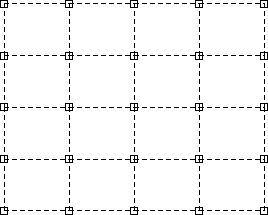
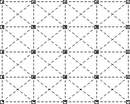
The common point of our examples is to select the hidden Gibbs model that better fits a given $y^{\text{obs}}$ composed of $N=100\times 100$ pixels within different neighborhood systems represented as undirected graphs $\mathscr{G}$. We considered the two widely used adjacency structures in our simulations, namely the graph $\mathscr{G}_{4}$ (respectively $\mathscr{G}_{8}$) in which the neighborhood of a site is composed of the four (respectively eight) closest sites on the two-dimensional lattice, except on the boundaries of the lattice, see Fig. 1. The prior probabilities of both models were set to $1/2$ in all experiments. The Bayesian analysis of the model choice question adds another integral beyond the two above mentioned sums that cannot be calculated explicitly or numerically either and the problem we illustrate are said triple intractable. Up to our knowledge the choice of the latent neighborhood structure has never been seriously tackled in the Bayesian literature. We mentioned here the mean field approximation of Forbes and Peyrard (2003) whose software can estimate paramaters of such models, and compare models fitness via a BIC criterion. But the first results we try to obtain with this tool were worse than with ABC, except for very low values of $\beta$. This means that either we did not manage to run the software properly, or that the mean field approximation is not appropriate to discriminate between neighborhood structures. The detailed settings of our three experiments are as follows.

First experiment.

We considered Potts models with $K=2$ colors and a noise process that switches each pixel independently with probability

$$\exp(-\alpha)/(\exp(\alpha)+\exp(-\alpha)),$$

following the proposal of Everitt (2012). The prior on $\alpha$ was uniform over $(0.42;2.3)$, where the bounds of the interval were determined to switch a pixel with a probability less than $30\%$. Regarding the dependency parameter $\beta$, we set prior distributions below the phase transition which occurs at different levels depending on the neighborhood structure. Precisely we used a uniform distribution over $(0;1)$ when the adjacency is given by $\mathscr{G}_{4}$ and a uniform distribution over $(0;0.35)$ with $\mathscr{G}_{8}$.

Second experiment.

We increased the number of colors in the Potts models and set $K=16$. Likewise, we set a noise that changes the color of each pixel with a given probability parametrized by $\alpha$, and conditionally on a change at site $i$, we rely on the least favorable distribution, which is a uniform draw within all colors except the latent one. To extend the parametrization of Everitt (2012), the marginal distribution of the noise is defined by

$$P_{\alpha}(y_{i}|x_{i})=\frac{\exp\Big{\{}\alpha\big{(}2\mathds{1}\{x_{i}=y_{i}\}-1\big{)}\Big{\}}}{\exp(\alpha)+(K-1)\exp(-\alpha)}$$

and a uniform prior on $\alpha$ over the interval $(1.78;4.8)$ ensures that the probability of changing a pixel with the noise process is at most $30\%$. The uniform prior on the Potts parameter $\beta$ was also tuned to stay below the phase transition. Hence $\beta$ ranges the interval $(0;2.4)$ with a $\mathscr{G}_{4}$ structure and the interval $(0;1)$ with a $\mathscr{G}_{8}$ structure.

Third experiment.

We introduced a homoscedastic Gaussian noise whose marginal distribution is characterized by

$$y_{i}\leavevmode\nobreak\ |\leavevmode\nobreak\ x_{i}=c\sim\mathcal{N}(c,\sigma^{2})\quad c\in\{0;1\}$$

over bicolor Potts models. And both prior distributions on parameter $\beta$ are similar to the ones on the latent fields of the first experiment. The standard deviation $\sigma=0.39$ was set so that the probability of a wrong prediction of the latent color with a marginal MAP rule on the Gaussian model is about $15\%$.

3.2 Geometric summary statistics

$\Gamma(\mathscr{G}_{4},y)$

$\Gamma(\mathscr{G}_{8},y)$

Figure 2: The induced graph $\Gamma(\mathscr{G}_{4},y)$ and $\Gamma(\mathscr{G}_{8},y)$ on a given bicolor image $y$ of size $5\times 5$. The six summary statistics on $y$ are thus $R(\mathscr{G}_{4},y)=22$, $T(\mathscr{G}_{4},y)=7$, $U(\mathscr{G}_{4},y)=12$, $R(\mathscr{G}_{8},y)=39$, $T(\mathscr{G}_{8},y)=4$ and $U(\mathscr{G}_{8},y)=16$

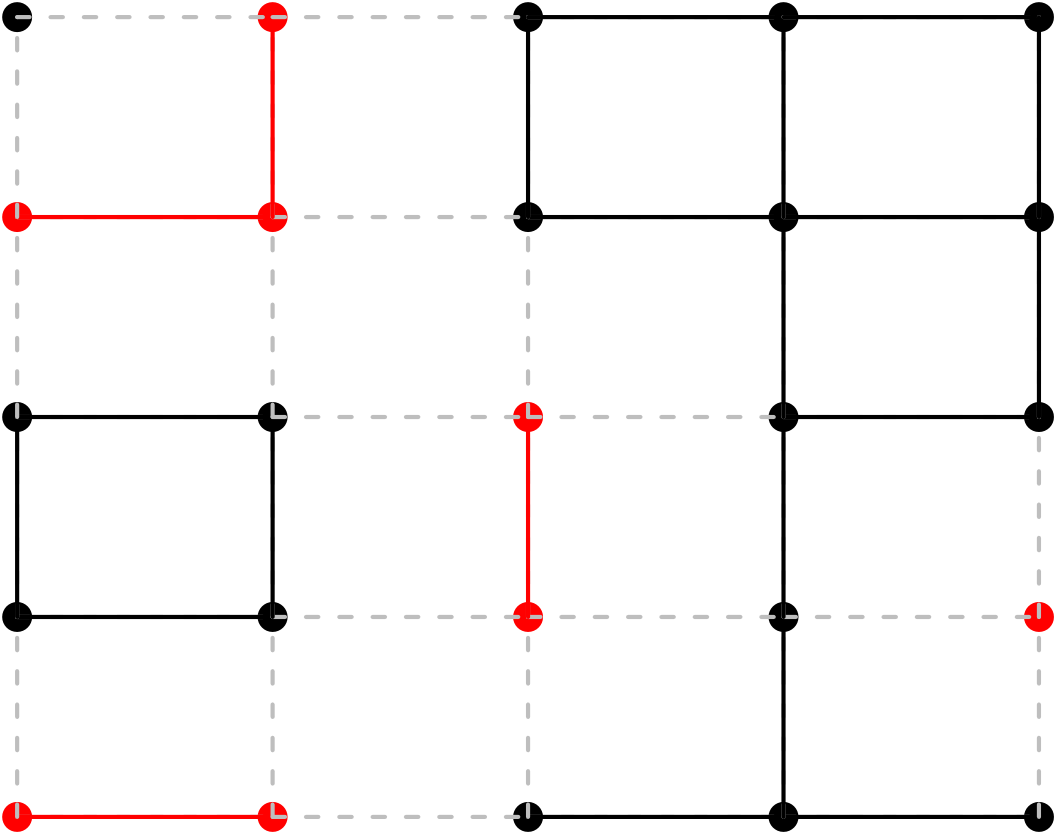
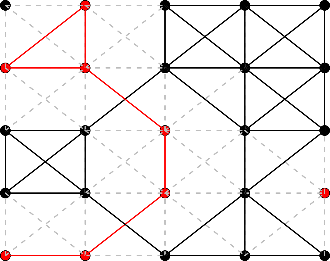
Performing a Bayesian model choice via ABC algorithms requires summary statistics that capture the relevant information from the observation $y^{\text{obs}}$ to discriminate among the competing models. When the observation is noise-free, Grelaud et al. (2009) noted that the joint distribution resulting from the Bayesian modeling falls into the exponential family, and they obtained consecutively a small set of summary statistics, depending on the collection of considered models, that were sufficient. In front of noise, the situation differs substantially as the joint distribution lies now outside the exponential family, and the above mentioned statistics are not sufficient anymore, whence the urge to bring forward other concrete and workable statistics. The general approach we developed reveals geometric features of a discrete field $y$ via the recourse to colored graphs attached to $y$ and their connected components. Consider an undirected graph $\mathscr{G}$ whose set of vertices coincides with $\mathscr{S}$, the set of sites of $y$.

Definition 4.

The graph induced by $\mathscr{G}$ on the field $y$, denoted $\Gamma(\mathscr{G},y)$, is the undirected graph whose set of edges gathers the edges of $\mathscr{G}$ between sites of $y$ that share the same color, i.e.,

$$i\stackrel{{\scriptstyle\Gamma(\mathscr{G},y)}}{{\sim}}j\quad\iff\quad i\stackrel{{\scriptstyle\mathscr{G}}}{{\sim}}j\text{ and }y_{i}=y_{j}.$$

We believe that the connected components of such induced graphs capture major parts of the geometry of $y$. Recall that a connected component of an undirected graph $\Gamma$ is a subgraph of $\Gamma$ in which any two vertices are connected to each other by a path, and which is connected to no other vertices of $\Gamma$. And the connected components form a partition of the vertices. Since ABC relies on the computation of the summary statistics on many simulated datasets, it is also worth noting that the connected components can be computed efficiently with the help of famous graph algorithms in linear time based on a breadth-first search or depth-first search over the graph. The empirical distribution of the sizes of the connected components represents an important source of geometric informations, but cannot be used as a statistic in ABC because of the curse of dimensionality. The definition of a low dimensional summary statistic derived from these connect components should be guided by the intuition on the model choice we face.

Our numerical experiments discriminate between a $\mathscr{G}_{4}$- and a $\mathscr{G}_{8}$-neighborhood structure and we considered two induced graphs on each simulated $y$, namely $\Gamma(\mathscr{G}_{4},y)$ and $\Gamma(\mathscr{G}_{8},y)$. Remark that the two-dimensional statistics proposed by Grelaud et al. (2009), which are sufficient in the noise-free context, are the total numbers of edges in both induced graphs. After very few trials without success, we fixed ourselves on four additional summary statistics, namely the size of the largest component of each induced graph, as well as the total number of connect components in each graph. See Fig. 2 for an example on a bicolor picture $y$. To fix the notations, for any induced graph $\Gamma(\mathscr{G},y)$, we define

• $R(\mathscr{G},y)$ as the total number of edges in $\Gamma(\mathscr{G},y)$,

• $T(\mathscr{G},y)$ as the number of connected components in $\Gamma(\mathscr{G},y)$ and

• $U(\mathscr{G},y)$ as the size of the largest connected component of $\Gamma(\mathscr{G},y)$.

And to sum up the above, the set of summary statistics that where registered in the reference tables for each simulated field $y$ is

$$S(y)=\Big{(}R(\mathscr{G}_{4},y);R(\mathscr{G}_{8},y);T(\mathscr{G}_{4},y);\\ T(\mathscr{G}_{8},y);U(\mathscr{G}_{4},y);U(\mathscr{G}_{8},y)\Big{)}$$

in the first and second experiments.

In the third experiment, the observed field $y$ takes values in $\mathbb{R}$ and we cannot apply directly the approach based on induced graphes because no two pixels share the same color. All of the above statistics are meaningless, including the statistics $R(\mathscr{G},y)$ used by Grelaud et al. (2009) in the noise-free case. We rely on a quantization preprocessing performed via a kmeans algorithm on the observed colors that forgets the spatial structure of the field. The algorithm was tuned to uncover the same number of groups of colors as the number of latent colors, namely $K=2$. If $q_{2}(y)$ denotes the resulting field, the set of summary statistics becomes

$$S(y)=\Big{(}R\big{(}\mathscr{G}_{4},q_{2}(y)\big{)};R\big{(}\mathscr{G}_{8},q_{2}(y)\big{)};T\big{(}\mathscr{G}_{4},q_{2}(y)\big{)};\\ T\big{(}\mathscr{G}_{8},q_{2}(y)\big{)};U\big{(}\mathscr{G}_{4},q_{2}(y)\big{)};U\big{(}\mathscr{G}_{8},q_{2}(y)\big{)}\Big{)}.$$

We have assumed here that the number of latent colors is known to keep the same purpose of selecting the correct neighborhood structure. Indeed Cucala and Marin (2013) have already proposed a (complex) Bayesian method to infer the appropriate number of hidden colors. But more generally, we can add statistics based on various quantizations $q_{k}(y)$ of $y$ with $k$ groups.

3.3 Numerical results

Table 1: Evaluation of the prior error rate on a test reference table of size $30,000$ in the first experiment.

Prior error rates

Train size	$\bf 5,000$	$\bf 100,000$
2D statistics	$8.8\%$	$7.9\%$
4D statistics	$6.5\%$	$6.1\%$
6D statistics	$7.1\%$	$7.1\%$
Adaptive ABC	$6.2\%$	$5.5\%$

(a)                                                             (b)                             

(c)

Figure 3: First experiment results. (a) Prior error rates (vertical axis) of ABC with respect to the number of nearest neighbors (horizontal axis) trained on a reference table of size $100,000$ (solid lines) or $50,000$ (dashed lines), based on the 2D, 4D and 6D summary statistics. (b) Prior error rates of ABC based on the 2D summary statistic compared with 4D and 6D summary statistics including additional ancillary statistics. (c) Evaluation of the local error on a 2D surface

In all three experiments, we compare three nested sets of summary statistics $S_{2D}(y)$, $S_{4D}(y)$ and $S_{6D}(y)$ of dimension 2, 4 and 6 respectively. They are defined as the projection onto the first two (respectively four and six) axes of $S(y)$ described in the previous section. We stress here that $S_{2D}(y)$, which is composed of the summaries given by Grelaud et al. (2009), are used beyond the noise-free setting where they are sufficient for model choice. In order to study the information carried by the connected components, we add progressively our geometric summary statistics to the first set, beginning by the $T(\mathscr{G},y)$-type of statistics in $S_{4D}(y)$. Finally, remark that, before evaluating the Euclidean distance in ABC algorithms, we normalize the statistics in each reference tables with respect to an estimation of their standard deviation since all these summaries take values on axis of different scales. Simulated images have been drawn thanks to the Swendsen and Wang (1987) algorithm. In the least favorable experiment, simulations of one hundred pictures (on pixel grid of size $100\times 100$) via $20,000$ iterations of this Markovian algorithm when parameters drawn from our prior requires about one hour of computation on a single CPU with our optimized C++ code. Hence the amount of time required by ABC is dominated by the simulations of $y$ via the Swedsen-Wang algorithm. This motivated Moores, Mengersen, and Robert (2014) to propose a cut down on the cost of running an ABC experiment by removing the simulation of an image from hidden Potts model, and replacing it by an approximate simulation of the summary statistics. Another alternative is the clever sampler of Mira et al. (2001) that provides exact simulations of Ising models and can be extended to Potts models.

First experiment.

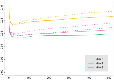
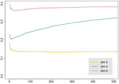
Fig. 3(a) illustrates the calibration of the number of nearest neighbors (parameter $k$ of Algorithm 2) by showing the evolution of the prior error rates (evaluated on a validation reference table including $20,000$ simulations) when $k$ increases. We compared the errors of six classifiers to inspect the differences between the three sets of summary statistics (in yellow, green and magenta) and the impact of the size of the training reference table ($100,000$ simulations in solid lines; $50,000$ simulations in dashed lines). The numerical results exhibit that a good calibration of $k$ can reduce the prior misclassification error. Thus, without really degrading the performance of the classifiers, we can reduce the amount of simulations required in the training reference table, whose computation cost (in time) represents the main obstacle of ABC methods, see also Table 1. Moreover, as can be guessed from Fig. 3(a), the sizes of the largest connected components of induced graphs (included only in $S_{6D}(y)$) do not carry additional information regarding the model choice and Table 1 confirms this results through evaluations of the errors on a test reference table of $30,000$ simulations drawn independently of both training and validation reference tables.

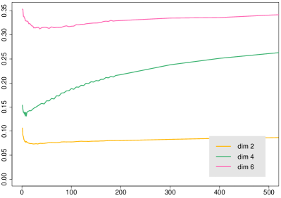
One can argue that the curse of dimensionality does not occur with such low dimensional statistics and sizes of the training set, but this intuition is wrong, as shown in Fig. 3(b). The latter plot shows indeed the prior misclassification rate as a function of $k$ when we replace the last four summaries by ancillary statistics drawn independently of $m$ and $y$. We can conclude that, although the three sets of summary statistics carry then the same information in this artificial setting, the prior error rates increase substantially with the dimension (classifiers are not trained on infinite reference tables!). This conclusion shed new light on the results of Fig. 3(a): the $U(\mathscr{G},y)$-type summaries, based on the size of the largest component, are not concretely able to help discriminate among models, but are either highly correlated with the first four statistics; or the resolution (in terms of size of the training reference table) does not permit the exploitation of the possible information they add.

Table 2: Evaluation of the prior error rate on a test reference table of size $20,000$ in the second experiment.

Prior error rates

Train size	$\bf 50,000$	$\bf 100,000$
2D statistics	$4.5\%$	$4.4\%$
4D statistics	$4.6\%$	$4.1\%$
6D statistics	$4.6\%$	$4.3\%$

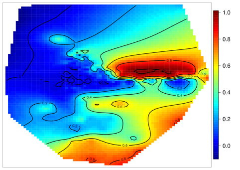
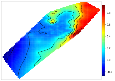
Fig. 3(c) displays the local error rate with respect to a projection of the image space on a plan. We have taken here $S_{1}(y)=S_{2D}(y)$ in Definition 2. And $S_{2}(y)$ ranges a plan given by a projection of the full set of summaries that has been tuned empirically in order to gather the errors committed by calls of $\widehat{m}(S_{2D}(y))$ on the validation reference table. The most striking fact is that the local error rises above $0.9$ in the oval, reddish area of Fig. 3(c). Other reddish areas of Fig. 3(c) in the bottom of the plot correspond to parts of the space with very low probability, and may be a dubious extrapolation of the Kriging algorithm. We can thus conclude that the information of the new geometric summaries depends highly on the position of $y$ in the image space and have confidence in the interest of Algorithm 4 (adaptive ABC) in this framework. As exhibited in Table 1(d), this last classifier does not decrease dramatically the prior misclassification rates. But the errors of the non-adaptive classifiers are already low and the error of any classifier is bounded from below, as explained in Proposition 3. Interestingly though, the adaptive classifier relies on $\widehat{m}(S_{2D}(y))$ (instead of the most informative $\widehat{m}(S_{6D}(y))$) to take the final decision at about $60\%$ of the images of our test reference table of size $30,000$.

Second experiment.

The framework was designed here to study the limitations of our approach based on the connected components of induced graphs. The number of latent colors is indeed relatively high and the noise process do not rely on any ordering of the colors to perturbate the pixels. Table 2 indicates the difficulty of capturing relevant information with the geometric summaries we propose. Only the sharpness introduced by a training reference table composed of $100,000$ simulations distinguishes $\widehat{m}(S_{4D}(y))$ and $\widehat{m}(S_{6D}(y))$ from the basic classifier $\widehat{m}(S_{2D}(y))$. This conclusion is reinforced by the low value of number of neighbors after the calibration process, namely $k=16,5$ and $5$ for $\widehat{m}(S_{2D}(y))$, $\widehat{m}(S_{4D}(y))$ and $\widehat{m}(S_{6D}(y))$ respectively. Hence we do not display in the paper other diagnosis plots based on the prior error rates or the conditional error rates, which led us to the same conclusion. The adaptive ABC algorithm did not improve any of these results.

Table 3: Evaluation of the prior error rate on a test reference table of size $30,000$ in the third experiment.

Prior error rates

Train size	$\bf 5,000$	$\bf 100,000$
2D statistics	$14.2\%$	$13.8\%$
4D statistics	$10.8\%$	$9.8\%$
6D statistics	$8.6\%$	$6.9\%$
Adaptive ABC	$8.2\%$	$6.7\%$

(a)                                                             (b)

(c)

Figure 4: Third experiment results. (a) Prior error rates (vertical axis) of ABC with respect to the number of nearest neighbors (horizontal axis) trained on a reference table of size $100,000$ (solid lines) or $50,000$ (dashed lines), based on the 2D, 4D and 6D summary statistics. (b) Prior error rates of ABC based on the 2D summary statistics compared with 4D and 6D summary statistics including additional ancillary statistics. (c) Evaluation of the local error on a 2D surface

Third experiment.

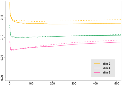
The framework here includes a continuous noise process as described at the end of Section 3.1. We reproduced the entire diagnosis process performed in the first experiment and we obtained the results given in Fig. 4 and Table 3. The most noticeable difference is the extra information carried by the $U(\mathscr{G},y)$-statistics, representing the size of the largest connected component, and the adaptive ABC relie on the simplest $\widehat{m}(S_{2D}(y))$ in about $30\%$ of the data space (measured with the prior marginal distribution in $y$). Likewise, the gain in misclassification errors is not spectacular, albeit positive.

4 Conclusion and perspective

In the present article, we considered ABC model choice as a classification problem in the framework of the Bayesian paradigm (Section 2.1) and provided a local error in order to assess the accuracy of the classifier at $y^{\text{obs}}$ (Sections 2.2 and 2.3). We derived then an adaptive classifier (Section 2.4) which is an attempt to fight against the curse of dimensionality locally around $y^{\text{obs}}$. This method contrasts with most projection methods which are focused on parameter estimation (Blum et al., 2013). Additionally, most of them perform a global trade off between the dimension and the information of the summary statistics over the whole prior domain, while our proposal adapts the dimension with respect to $y^{\text{obs}}$ (see also the discussion about the posterior loss approach in Blum et al., 2013). Besides the inequalities of Proposition 3 complement modestly the analysis of Marin et al. (2013) on ABC model choice. Principles of our proposal are well founded by avoiding the well-known optimism of the training error rates and by resorting to validation and test reference tables in order to evaluate the error practically. And, finally, the machine learning viewpoint gives an efficient way to calibrate the threshold of ABC (Section 2.1).

Regarding latent Markov random fields, the proposed method of constructing summary statistics based on the induced graphs (Section 3.2) yields a promising route to construct relevant summary statistics in this framework. This approach is very intuitive and can be reproduced in other settings. For instance, if the goal of the Bayesian analysis is to select between isotropic latent Gibbs models and anisotropic models, the averaged ratio between the width and the length of the connect components or the ratio of the width and the length of the largest connected components can be relevant numerical summaries. We have also explained how to adapt the method to a continuous noise by performing a quantization of the observed values at each site of the fields (Section 3.2). And the detailed analysis of the numerical results demonstrates that the approach is promising. However the results on the $16$ color example with a completely disordered noise indicate the limitation of the induced graph approach. We believe that there exists a road we did not explore above with an induced graph that add weights on the edges of the graph according to the proximity of the colors, but the grouping of sites on such weighted graph is not trivial.

The numerical results (Section 3.3) highlighted that the calibration of the number of neighbors in ABC provides better results (in terms of misclassification) than a threshold set as a fixed quantile of the distances between the simulated and the observed datasets (as proposed in Marin et al., 2012). Consequently, we can reduce significantly the number of simulations in the reference table without increasing the misclassification error rates. This represents an important conclusion since the simulation of a latent Markov random field requires a non-negligible amount of time. The gain in misclassification rates of the new summaries is real but not spectacular and the adaptive ABC algorithm was able to select the most performant classifier.

References

- Alfò et al. [2008] M. Alfò, L. Nieddu, and D. Vicari. A finite mixture model for image segmentation. Statistics and Computing, 18(2):137–150, 2008.
- Baragatti and Pudlo [2014] M. Baragatti and P. Pudlo. An overview on Approximate Bayesian Computation. ESAIM: Proc., 44:291–299, 2014.
- Beaumont et al. [2009] M. A. Beaumont, J.-M. Cornuet, J.-M. Marin, and C. P. Robert. Adaptive approximate Bayesian computation. Biometrika, page asp052, 2009.
- Besag [1974] J. Besag. Spatial interaction and the statistical analysis of lattice systems (with Discussion). Journal of the Royal Statistical Society. Series B (Methodological), 36(2):192–236, 1974.
- Besag [1975] J. Besag. Statistical Analysis of Non-Lattice Data. The Statistician, 24:179–195, 1975.
- Biau et al. [2013] G. Biau, F. Cérou, and A. Guyader. New insights into Approximate Bayesian Computation. Annales de l’Institut Henri Poincaré (B) Probabilit s et Statistiques, in press, 2013.
- Blum et al. [2013] M. G. B. Blum, M. A. Nunes, D. Prangle, and S. A. Sisson. A Comparative Review of Dimension Reduction Methods in Approximate Bayesian Computation. Statistical Science, 28(2):189–208, 2013.
- Caimo and Friel [2011] A. Caimo and N. Friel. Bayesian inference for exponential random graph models. Social Networks, 33(1):41–55, 2011.
- Caimo and Friel [2013] A. Caimo and N. Friel. Bayesian model selection for exponential random graph models. Social Networks, 35(1):11 – 24, 2013.
- Cucala and Marin [2013] L. Cucala and J.-M. Marin. Bayesian Inference on a Mixture Model With Spatial Dependence. Journal of Computational and Graphical Statistics, 22(3):584–597, 2013.
- Del Moral et al. [2012] P. Del Moral, A. Doucet, and A. Jasra. An adaptive sequential monte carlo method for approximate bayesian computation. Statistics and Computing, 22(5):1009–1020, 2012.
- Devroye et al. [1996] L. Devroye, L. Györfi, and G. Lugosi. A probabilistic theory of pattern recognition, volume 31 of Applications of Mathematics (New York). Springer-Verlag, New York, 1996.
- Didelot et al. [2011] X. Didelot, R. G. Everitt, A. M. Johansen, and D. J. Lawson. Likelihood-free estimation of model evidence. Bayesian Analysis, 6(1):49–76, 2011.
- Druilhet and Marin [2007] P. Druilhet and J.-M. Marin. Invariant HPD credible sets and MAP estimators. Bayesian Analysis, 2(4):681–691, 2007.
- Estoup et al. [2012] A. Estoup, E. Lombaert, J.-M. Marin, C. Robert, T. Guillemaud, P. Pudlo, and J.-M. Cornuet. Estimation of demo-genetic model probabilities with Approximate Bayesian Computation using linear discriminant analysis on summary statistics. Molecular Ecology Ressources, 12(5):846–855, 2012.
- Everitt [2012] R. G. Everitt. Bayesian Parameter Estimation for Latent Markov Random Fields and Social Networks. Journal of Computational and Graphical Statistics, 21(4):940–960, 2012.
- Forbes and Peyrard [2003] F. Forbes and N. Peyrard. Hidden Markov random field model selection criteria based on mean field-like approximations. Pattern Analysis and Machine Intelligence, IEEE Transactions on, 25(9):1089–1101, 2003.
- François et al. [2006] O. François, S. Ancelet, and G. Guillot. Bayesian Clustering Using Hidden Markov Random Fields in Spatial Population Genetics. Genetics, 174(2):805–816, 2006.
- Friel [2012] N. Friel. Bayesian inference for Gibbs random fields using composite likelihoods. In Simulation Conference (WSC), Proceedings of the 2012 Winter, pages 1–8, 2012.
- Friel [2013] N. Friel. Evidence and Bayes Factor Estimation for Gibbs Random Fields. Journal of Computational and Graphical Statistics, 22(3):518–532, 2013.
- Friel and Rue [2007] N. Friel and H. Rue. Recursive computing and simulation-free inference for general factorizable models. Biometrika, 94(3):661–672, 2007.
- Friel et al. [2009] N. Friel, A. N. Pettitt, R. Reeves, and E. Wit. Bayesian Inference in Hidden Markov Random Fields for Binary Data Defined on Large Lattices. Journal of Computational and Graphical Statistics, 18(2):243–261, 2009.
- Green and Richardson [2002] P. J. Green and S. Richardson. Hidden Markov Models and Disease Mapping. Journal of the American Statistical Association, 97(460):1055–1070, 2002.
- Grelaud et al. [2009] A. Grelaud, C. P. Robert, J.-M. Marin, F. Rodolphe, and J.-F. Taly. ABC likelihood-free methods for model choice in Gibbs random fields. Bayesian Analysis, 4(2):317–336, 2009.
- Hurn et al. [2003] M. A. Hurn, O. K. Husby, and H. Rue. A Tutorial on Image Analysis. In Spatial Statistics and Computational Methods, volume 173 of Lecture Notes in Statistics, pages 87–141. Springer New York, 2003. ISBN 978-0-387-00136-4.
- Marin et al. [2012] J.-M. Marin, P. Pudlo, C. P. Robert, and R. J. Ryder. Approximate Bayesian Computational methods. Statistics and Computing, 22(6):1167–1180, 2012.
- Marin et al. [2013] J.-M. Marin, N. S. Pillai, C. P. Robert, and J. Rousseau. Relevant statistics for Bayesian model choice. Journal of the Royal Statistical Society: Series B (Statistical Methodology), 2013.
- Marjoram et al. [2003] P. Marjoram, J. Molitor, V. Plagnol, and S. Tavaré. Markov chain Monte Carlo without likelihoods. Proceedings of the National Academy of Sciences, 100(26):15324–15328, 2003.
- Mira et al. [2001] A. Mira, J. Møller, and G. O. Roberts. Perfect slice samplers. Journal of the Royal Statistical Society: Series B (Statistical Methodology), 63(3):593–606, 2001.
- Moores et al. [2014] M. T. Moores, C. E. Hargrave, F. Harden, and K. Mengersen. Segmentation of cone-beam CT using a hidden Markov random field with informative priors. Journal of Physics : Conference Series, 489, 2014.
- Moores et al. [2014] M. T. Moores, K. Mengersen, and C. P. Robert. Pre-processing for approximate Bayesian computation in image analysis. ArXiv e-prints, March 2014.
- Prangle et al. [2013] D. Prangle, P. Fearnhead, M. P. Cox, P. J. Biggs, and N. P. French. Semi-automatic selection of summary statistics for ABC model choice. Statistical Applications in Genetics and Molecular Biology, pages 1–16, 2013.
- Pritchard et al. [1999] J. K. Pritchard, M. T. Seielstad, A. Perez-Lezaun, and M. W. Feldman. Population growth of human Y chromosomes: a study of Y chromosome microsatellites. Molecular Biology and Evolution, 16(12):1791–1798, 1999.
- Reeves and Pettitt [2004] R. Reeves and A. N. Pettitt. Efficient recursions for general factorisable models. Biometrika, 91(3):751–757, 2004.
- Robert et al. [2011] C. P. Robert, J.-M. Cornuet, J.-M. Marin, and N. S. Pillai. Lack of confidence in approximate Bayesian computation model choice. Proceedings of the National Academy of Sciences, 108(37):15112–15117, 2011.
- Swendsen and Wang [1987] R. H. Swendsen and J.-S. Wang. Nonuniversal critical dynamics in Monte Carlo simulations. Physical Review Letters, 58(2):86–88, 1987.
- Tavaré et al. [1997] S. Tavaré, D. J. Balding, R. C. Griffiths, and P. Donnelly. Inferring Coalescence Times From DNA Sequence Data. Genetics, 145(2):505–518, 1997.