Adapted Basis for Non-Local
Reconstruction of Missing Spectrum
Abstract
The object of this work is to design an adequate regularization for the problem of recovering missing Fourier coefficients, particularly in some non standard situations were low frequency coefficients are lost. In the framework of non-local regularization, we propose a technique to build an original patchwise similarity measure that is adapted to the missing spectrum. Then, a simple Non-Local quadratic energy is minimized. By construction, the similarity criterion is invariant under the corruption process so that the distance between two patches of the corrupted image is almost exactly equal to the one computed on the clean image. We illustrate our method with experiments which show its efficiency, both in terms of speed and quality of the results, with respect to other common approaches. We show that the method is practical on synthetic examples which are built upon models of inverse scattering problems, synthetic aperture mirrors for spatial imaging or also medical imaging.
1 Introduction
In this paper, we consider the problem of retrieving missing Fourier coefficients of a raw data. This problem has important applications in various fields:
-
•
The zooming problem in image processing where one has to construct high frequency data from a low-resolution sample. This is of some importance nowadays for the transition of SD videos to HD ones.
- •
-
•
The tomography problem for medical imaging or seismic imaging. In this case Fourier coefficients usually lie on straight lines that are either parallel or that cross at the origin.
-
•
The inverse scattering problem where one is interested in recovering the shape of an hidden object using electromagnetic or acoustic waves.
Let us consider the latter example (see [7] for details). Let an incident acoustic plane wave propagate in the direction of the unit vector in an isotropic medium. Here is the wave number. In case there is an inhomogeneity (the hidden object), the wave will be “scattered” and give rise to another wave . The latter has an asymptotic behavior
| (1) |
where is known as the far field pattern and gives an idea of the behavior of the scattered wave at large distance. Here, is the observation direction and is the incident wave direction. The direct problem amounts to find whereas the nonlinear inverse problem takes the direct method as a starting point and asks what is the nature of the scatterer that gave rise to such a farfield. In what follows, we assume that is sufficiently small so that the Born approximation implies that
| (2) |
This means that can be interpreted as Fourier coefficients in the ball of radius . In practice, having only limited incident waves and measurements we end up with a sampling of the spectrum of that is depicted in Fig. 2.

In general non regular sampling of the spectrum is a difficult problem (see for instance [23]). Though if is bounded, its Fourier transform is a function that can be interpolated on a uniform grid. This allows to use the fft.
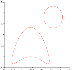
In [14, 24], the authors consider the Total Variation (henceforth denoted ) to recover missing Fourier coefficients. Let us compare the performance of this approach with that of the factorization method [21] thanks to a numerical test. We consider the object that is bounded by the red curves in Fig. 2. The inverse problem is then solved given 32 incident waves and 32 measurement directions. The wave number is . The factorization method, which performs quite well for small values of , yields quite poor results in this extreme case:
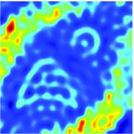
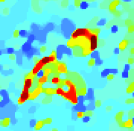
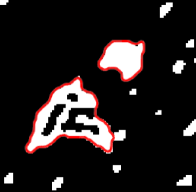
The -based method yields really good results in this case. Indeed, from partial and noisy measurements, we were able to distinguish two objects that are merely separated by where is the wavelength. This value is close to the theoretical diffraction limit that is . Note also it is not necessary to tune a Lagrange multiplier as it is usually done. Indeed, if one denotes the discrete set of points where is known, one can simply minimize the constrained problem
| (3) |
to get the restoration shown in Fig. 3.
Total Variation was already used for solving the nonlinear inverse scattering problem in [29]. The idea of considering the inverse problem within the Born approximation as an inpainting problem in the Fourier domain is discussed in [10].
This example shows that using variational methods for the general spectrum interpolation problem may yield quite satisfactory results. We should also mention the not so different problem of restoring missing wavelet coefficients which is treated in [5, 30]. For such problems, can we do better than using ? Some recent papers address the problem of solving general inverse problems in imaging by means of non-local methods. These methods obviously apply to the problem of retrieving missing Fourier coefficients.
2 Prior Works
Traditional methods in image processing are based on local properties of images (Wavelets, Total Variation). Recently, state of the art results were achieved for the denoising problem by Non-Local methods that exploit redundancies in images. The idea of using self-similarities in images was first exploited in [3]. They proposed a filter that averages similar patterns of a noisy image defined on even though these self-similarities occur at large distance. The filter reads as follows
| (4) |
where are patches of and determines the selectivity of the similarity measure. Many modifications of this filter were considered for denoising purposes (adaptive , adaptive window [19], shape adaptive patches [9]).
The use of patches has been widely adopted in the image processing community and in the recent years, these non-local methods were extended to the study of general inverse problems (see [20, 13, 12, 26, 1]). Such a general inverse problem can be modeled as follows Here is the original image defined on , is a linear transformation and is a white Gaussian noise. The classical local methods were adapted by considering a pointwise Non-Local regularization as introduced in [13]
| (5) |
for some and where is the weight function used in the NLMeans filter and is based on the Sum of Squared Differences (henceforth called SSD distance). As for , it is a function of compact support centered at the origin. It indicates that patches that are too far from each other should not be taken into account. Indeed, it was observed that the Non-Local methods yield much better results if one seeks for similar patches in the support of , referred to as the search window (see also assumption in Section 7).
Peyré et al. proposed in [27] (see also [1]) a patchwise Non-Local regularization
| (6) |
To get a restored image one then has to minimize the following Non-Local energy
| (7) |
It is further remarked that one can enhance the restoration by recomputing the weight regularly. In [1, 27], the authors proposed a general framework where the weight is interpreted up to renormalization as a density of probability and is an unknown of the problem. Then the energy to be minimized involves the potential energy of , used to infer unknown probability distributions. The resulting energy is not convex in and an alternate coordinate descent gives back the SSD-based weight but computed this time on the being processed. This actually corresponds to the aforementioned weight recomputation procedure.
3 Contribution
In this paper, we deal with the problem of restoring missing Fourier coefficients of an image. In particular we propose a technique to build a distance insensitive to the degradation of an image. The corruption process is supposed to be known. We show that using this distance between patches gives very good reconstruction results by solving a simple quadratic energy.
In the classical Non-Local approaches, a critical step is to compute the SSD distance between two patches of the corrupted image. This strategy dates back to the NLMeans [3].We explain how to replace this step by the computation of a simpler -type distance that is really adapted to the problem of spectrum reconstruction and does not incorporate spurious information. The idea is to define atoms similar to Gabor filters to test whether two regions of the corrupted image are similar. These atoms should be as concentrated as possible and should not depend on the corruption process. This way two patches that are close in the clean image will be close in the corrupted image. We now first introduce our variational framework, which is relatively standard.
4 A Non-Local Energy for the Problem
Henceforth, we work in which will is equipped with the norm so that “balls” are in fact squares.
In this section, we first formalize the problem of reconstructing unknown coefficients of a Fourier series. Let us call the finite mask of points where the Fourier coefficients are known. We shall assume that it is symmetric with respect to the origin. Assuming that the image is periodic and defined on , one thus considers respectively the clean image and the corrupted images
| (8) |
We assume that not only the high frequencies but also middle range frequencies are lost in the corruption process. In other words, we keep the Fourier coefficients corresponding to the white areas of the mask . The typical we will consider here is the following

for which usual local TV-based reconstruction techniques totally fail at recovering the middle-range frequencies, see for instance Fig. 5, right.
In the sequel, we introduce the two subsets of : and its complement where in both cases runs over all sequences in , which are even in . Let us denote the orthogonal projection on . We recall that the Fourier transform on the torus is an isometry and thus invertible so the corrupted data that one has to interpolate is obtained by
| (9) |
We shall call patch centered at , denoted , the image where is a test function with support and is the patch size.
For the moment let us assume that the original image is such that there are two distinct with This is to say that two patches are similar in the original image. Then clearly, the part of the image corresponding to the missing frequencies is among the solutions of
| (10) |
where is smooth and such that , and is fixed. This means that knowing that and are similar one can hope to get a restored spectrum by minimizing (10). The reconstruction is obviously not unique since modifying out of does not change the energy (and numerical simulations actually show that the reconstructed has the same support as ). Thus, we have to take into account all the patches in the image to get a global reconstruction.
We are therefore led to consider the following problem
| (11) |
where and , that is going to be defined in the sequel, should tell us from the corrupted image whether one had for the original image
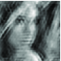
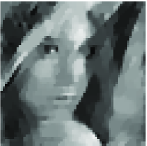
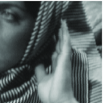
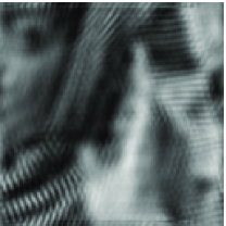
There are two interesting values for , namely and . Our first experiment (Fig. 5) shows that the reconstruction with (11) for both these choices is almost perfect if the weights are derived from the “oracle” distance given by the SSD distance of the patches of the (normally unknown) original image .
| Original image | Corrupted image |
 |
 |
| PSNR=20.0dB |
| Oracle () | Oracle () | TV restored |
 |
 |
 |
| PSNR=25.6dB | PSNR=26.2dB | PSNR=20.9dB |
| Original image | Corrupted image |
 |
 |
| PSNR=24.1dB |
| Oracle () | Oracle () | TV restored |
 |
 |
 |
| PSNR=28.9dB | PSNR=29.5dB | PSNR=24.5dB |
From these experiments, it seems clear that both values of allowed us to produce a cleaner image. Due to the huge size of our problems, we will stick in general to the case of the exponent which de facto excludes the case of standard Non-Local Total Variation. We will see that this choice leads to computationally tractable problems with excellent results, for some masks (such as the one in Fig. 4), provided the distance between similar patches is correctly estimated. For the considered mask (Fig. 4), standard Total Variation yield low quality reconstructions (right).
5 Construction of Atoms Adapted to the Corruption
Our aim is to define a similarity measure for patches that is not modified through the corruption process . This way, if two points are close in the original image they will remain close in the perturbed image.
To do so, our idea is to find a family of test functions dense in , that do not depend on and such that
| (12) |
The atoms should obviously depend on the mask . Indeed, for any ,
| (13) |
which means that and therefore for any . From the uncertainty principle (see [22]), one knows that is not of compact support (since M is) but one could still expect it to be localized in space. This can be ensured by defining these functions as minimizers of the following parameterized problems
| (14) |
where we minimize the -moments of , for some .
We can then consider a measure of similarity that is of the form
| (15) |
where sets how localized the considered atoms are. Now, by definition, the similarity measure is invariant under the corruption process . In other words, two patches that were identical in the original image may not necessarily match according to the SSD but will match according to the atom-based distance, provided that the atoms are well localized.
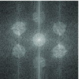
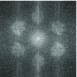
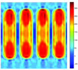
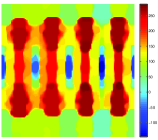
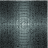
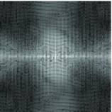
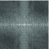
For the mask of Fig. 4, the first atoms are actually really localized and can be used as test functions. Let us have a closer look at the 7 first atoms, computed for , with their respective spectra:


These atoms adapted to the mask may recall the reader of the Gabor atoms (see [22]). However, they have the advantage of having a prescribed spectrum and being as localized as possible. They are in a sense the optimal functions satisfying these two conditions (see Section 7 for a discussion on the numerical algorithms that can be used in the discrete setting to compute these atoms.)
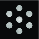
Let us now consider the following synthetic image:


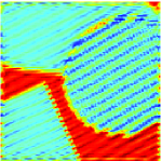
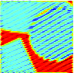
In Fig. 8, we can see that these atoms behave as Gabor atoms by capturing different patterns in the corrupted image. The different regions of can thus be distinguished by analyzing the filtered .

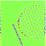

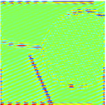
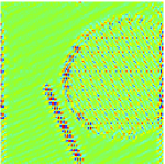
The previous atoms were computed for the mask considered in Fig. 4. However, our approach is quite general and can be adapted to any other corruption mask. As an example, here follow the atoms we get if we consider the mask that comes into play in the scattering problem:


These atoms are also really localized and are about the same size as a classical image patch (about 10 pixels wide) which therefore allows us to correlate local features of an image within a Non-Local approach.
6 Distance Map Comparison
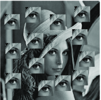
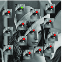
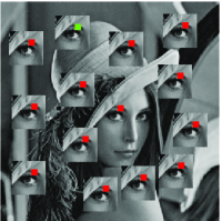
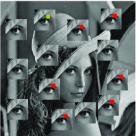
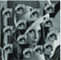
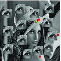
We are going to compare the performance of the different similarity measures considered so far by fixing one patch of the corrupted image (indicated in green in the clean image) and identify the best matches in the corrupted image (and indicated in red in the clean image) according to
-
The atom-based distance .
-
The ideal distance based on the clean .
-
The SSD .
| Original and corrupted | Atom-based | Oracle | SSD |
|---|---|---|---|
 |
 |
 |
 |
 |
 |
 |
 |
The two lines correspond to two different choices for the patch or reference (first line: a small square on the eyebrow from the second large eye patch, second line: the edge of the hat towards the middle) The second and fourth columns are computed using the corrupted image . The results are displayed on the clean image. In the third column we depicted the results obtained with the SSD computed with the clean image.
These two examples suggest that the atom-based distance we designed performs better than the SSD in some cases: indeed, the atom based results are closer to the “oracle” than the SSD which looses more matches.
7 Numerical Experiment
From now on, we are going to make important assumptions that let us drastically improve the complexity of the minimization problem (11) and save memory:
-
Two patches are unlikely to be the same if they are far from each other thus we can assume that for any fixed , is a candidate if for some fixed . This defines a neighborhood of candidates (also called window).
-
Once computed, we can for any fixed pixel keep only the best matches (see Fig. 10).
Weight computation:
Notice that for a fixed mask , the atoms can be computed in advance and stored. Then can be readily, computed once for all, using the fft. Now, we recall that
| (16) | ||||
| (17) |
From the previous definitions, it is readily seen that if or pixels is the patch size, then, as far as 111which will always be the case, otherwise it means that all atoms are essentially compactly supported which is possible only if the mask is full, it is faster to compute . In practice, this can result in an acceleration of order 10. Such a gain in complexity will be observed numerically in the sequel.
Algorithmic issues: An interesting feature of our work is that most optimization problems which are solved are constrained quadratic minimizations. Thus, the best choice (which we used) is the conjugate gradient. We also used Beck-Teboulles’s algorithm [2] in some instances, since our same program was optionally implementing an additional TV-regularization, with no real difference. The assumptions allow us to accelerate the computation.
Numerical results: In the following tests we consider three different energies:
- •
-
•
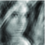
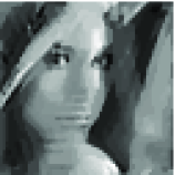
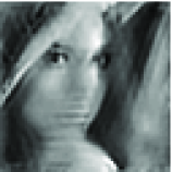
The constrained minimization problem (11) where we consider the SSD measure of similarity . In the simulations of Fig. 12 and Fig. 13, we take the window size pixels, the patch size pixels and pixels. For a fixed patch, we only keep the best matches and . For the tests of Fig. 14-18, we set , , , , . For the smaller example of Fig. 11 we chose , , , , . In Fig. 19 we chose , , , , .
-
•
The constrained minimization problem (11) where the weight is computed with the atom-based distance . In the tests of Fig. 12 and Fig. 13, we consider the first atoms with a moment . As above we take pixels, and for a fixed patch, we only consider the best matches. For Fig. 14-17, we set , , , , , . To produce Fig. 19 we took , , , , , . For the small image of Fig. 11 we picked , , , , , .
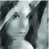
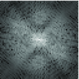
| Original | Corrupted |
 |
 |
| PSNR=20.0dB |
| SSD - | SSD - | NL-Atom - | NL-Atom - | |
| TV restored | ||||
 |
 |
 |
 |
 |
| PSNR=21.1dB | PSNR=20.7dB | PSNR=21.3dB | PSNR=21.1dB | PSNR=20.9dB |
 |
 |
 |
 |
 |
For this first example, both choices for the parameter provide improved results. The minimization is possible either by approximating the norm or by using modern splitting algorithms as introduced in [28, 8].
In this experiment, it is interesting to observe that the robust choice is particularly useful with the SSD distance which is likely to produce outliers (spurious matches), and almost useless with the oracle distance (see Fig. 5) which produces perfect matches. Our distance seems to lie in-between, in a region where the choice is apparently less decisive.
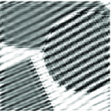
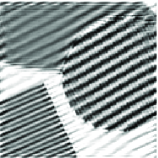
Henceforth, we shall only consider the exponent which is numerically tractable for larger images (the case being in practice, as expected, quite slower than the quadratic case). The experiment that follows (Fig. 12) is a simple but larger toy example.
| Original | Corrupted | SSD - | NL-Atom - | TV restored |
 |
 |
 |
 |
 |
| PSNR=8.5dB | PSNR=9.2dB | PSNR=10.6dB | PSNR=8.4dB | |
 |
 |
 |
 |
 |
| Original | Corrupted | SSD - | NL-Atom - | TV restored |
 |
 |
 |
 |
 |
| PSNR=24.0dB | PSNR=24.6dB | PSNR=24.7dB | PSNR=24.1dB | |
 |
 |
 |
 |
 |
Fig. 12 and 13 show an example with the
Mask of Fig. 4. In this case, the best results
are obtained with the atom-based distance. In particular in Fig. 12,
the oscillations with frequencies in the mask are almost perfectly
recovered and the spurious contamination is very low.
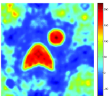
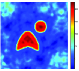
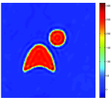
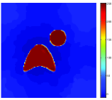
Let us see how these methods perform for the acoustic scattering problem of Section 1. To do so, we consider the mask introduced in Fig. 2.
| Original | Corrupted | SSD - | NL-Atom - | TV restored |
 |
 |
 |
 |
 |
| PSNR=14.4dB | PSNR=18dB | PSNR=24.5dB | PSNR=29.1dB | |
 |
 |
 |
 |
 |
In this case the best results are obtained with the standard Total Variation: this is consistent with the fact that the object to recover is piecewise constant and the loss is mostly in the high frequencies (for further details on these qualitative properties see [15, 16, 17]).
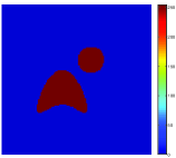
In the next simulation, we are going to assume that the Fourier coefficients that we kept are contaminated by a Gaussian noise of magnitude .
| Original | Corrupted | SSD - | NL-Atom - | TV restored |
 |
 |
 |
 |
 |
| PSNR=13.4dB | PSNR=13.6dB | PSNR=17.1dB | PSNR=14.4dB | |
 |
 |
 |
 |
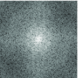 |
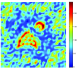
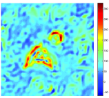
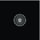
In this case, the Total Variation based optimization find it much harder to recover the data and the Atom-based distance yields satisfactory results. Now considering the Born approximation (2), let us use the data that comes out of the direct problem. In a sense, this amounts to adding to the Fourier coefficients a noise whose distribution is unknown. Our method is able to get rid of all the spurious objects.
| Original | Corrupted | SSD - | NL-Atom - | TV restored |
 |
 |
 |
 |
 |
| PSNR=9.24dB | PSNR=9.25dB | PSNR=9.81dB | PSNR=9.42dB | |
 |
 |
 |
 |
 |
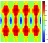
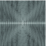
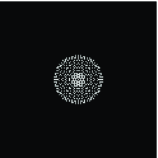
In this kind of problems it is usually important to distinguish objects that are very close. Let us consider such a situation:
| Original | Corrupted | SSD - | NL-Atom - | TV restored |
 |
 |
 |
 |
 |
| PSNR=8.2dB | PSNR=8.4dB | PSNR=14.5dB | PSNR=9.6dB | |
 |
 |
 |
 |
 |
Actually, in the latter experiment, we were able to distinguish objects that are separated by which is quite close to the theoretical limit . We were able to achieve this result since, we recall, two identical patches in the original image do not necessarily match according to the SSD but do match according to the atom-based distance. This explains why in Fig. 17, the atom-based distance improves the matching step (as in Fig. 10) and provides logically better results as observed in the different tests. In this case, there is to our knowledge no method but the one we propose to improve the results over the raw data.
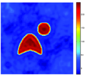
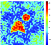
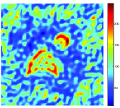
Weight recomputation: In [11, 12, 26, 27, 1], it was pointed out that one can get improved results (especially for inpainting problems) by allowing recomputation of the SSD-based weight on the being restored image. We depict in Fig. 18 the restorations one can expect after several recomputations.
 |
 |
 |
| PSNR=12.1dB | PSNR=24.9dB | PSNR=22.3 dB |
 |
 |
 |
| PSNR=14.6dB | PSNR=9.27dB | PSNR=8.9dB |
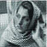
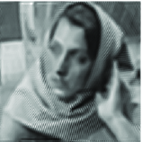
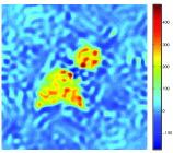
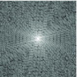
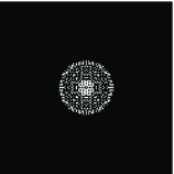
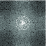
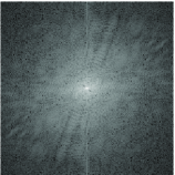
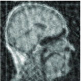
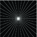
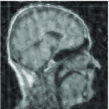
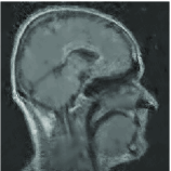
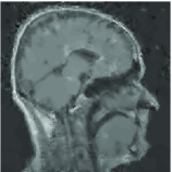
This procedure is really cumbersome and does not always improve results over the atom-based method. The weight recomputation is not possible for the atom-based distance we introduced since the distance computed on the restored image is exactly the same as the one computed on the corrupted image. However, our method can be used as an initialization for the classical weight recomputation to improve results further. This is the strategy we adopt in the following tomography problem where the Fourier coefficients got corrupted by a Gaussian noise of magnitude :
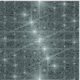
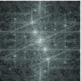
| Original | Spectrum of | Corrupted | Spectrum of |
 |
 |
 |
 |
| PSNR=22.4dB |
| then one | recomputed | |||
| SSD - | NL-Atom - | computation of | 20 times | TV restored |
 |
 |
 |
 |
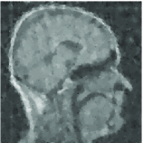 |
| PSNR= 23.8dB | PSNR=24.9dB | PSNR=25.8dB | PSNR=24.8dB | PSNR=23.6dB |
Computation Times: As we claimed previously in our discussion on complexity, the computation time with our approach (which in a first step reduces the dimensionality to retain only the information which is useful for the matching) is quite reduced. For instance, in Fig. 19 we observed the following computation times
| Approach | Computation time |
|---|---|
| SSD - | 83s (dist) + 15s (iter) = 98s |
| NL-Atom - | 8s (dist) + 25s (iter) = 33s |
| then one | 143s |
| recomputed 20 times | 30min |
| restored | 82s |
We performed our experiments in Matlab, so the absolute CPU times are not really relevant.
8 Conclusion
In this paper, we have considered the problem of reconstructing an image with a known pattern of missing Fourier coefficients, by means of a non-local method which assumes and exploits some spatial redundancy of the original image. In order to detect similar patches on the original image, we have introduced an original similarity criterion which is different from a standard quadratic distance, and is insensitive to the image degradation. This distance is based on precomputed atoms which are then used to filter out the degradation of the image, without destroying the local features.
Then, by minimizing a simple variational model (based on a quadratic energy, which we claim would produce the exact solution if the similar patches were exactly known—and in large enough quantity), we have experimentally shown the efficiency of this non-local framework, for some Fourier pattern. If the loss of coefficients is only in the high frequencies, then our approach does not produce any improvement over standard zooming techniques (local or nonlocal). On the other hand, for more complex masks which miss low frequency Fourier coefficients, our results are far superior to results obtained with more usual measures of redundancy.
References
- [1] P. Arias, G. Facciolo, V. Caselles, and G. Sapiro, A variational framework for exemplar-based image inpainting, International journal of computer vision, (2011).
- [2] Amir Beck and Marc Teboulle, A fast iterative shrinkage-thresholding algorithm for linear inverse problems, SIAM J. Imaging Sci., 2 (2009), pp. 183–202.
- [3] A. Buades, B. Coll, and Jean-Michel Morel, A non-local algorithm for image denoising, in CVPR 2005, vol. 2, IEEE, 2005.
- [4] Antonin Chambolle and Thomas Pock, A first-order primal-dual algorithm for convex problems with applications to imaging, J. Math. Imaging Vision, 40 (2011), pp. 120–145.
- [5] Tony Chan, Jianhong Shen, and Hao-Min Zhou, Total variation wavelet inpainting, J. Math. Imaging Vision, 25 (2006), pp. 107–125.
- [6] T. Chan and L.A. Vese, Active contours without edges, Image Processing, IEEE Transactions on, 10 (2001), pp. 266–277.
- [7] David Colton, Inverse acoustic and electromagnetic scattering theory, in Inside out: inverse problems and applications, vol. 47 of Math. Sci. Res. Inst. Publ., Cambridge Univ. Press, Cambridge, 2003, pp. 67–110.
- [8] Patrick L Combettes and Jean-Christophe Pesquet, Proximal splitting methods in signal processing, in Fixed-Point Algorithms for Inverse Problems in Science and Engineering, Springer, 2011, pp. 185–212.
- [9] Kostadin Dabov, Alessandro Foi, Vladimir Katkovnik, Karen Egiazarian, et al., BM3D image denoising with shape-adaptive principal component analysis, in SPARS’09-Signal Processing with Adaptive Sparse Structured Representations, 2009.
- [10] AJ Devaney, Inversion formula for inverse scattering within the born approximation, Optics Letters, 7 (1982), pp. 111–112.
- [11] G. Gilboa, J. Darbon, S. Osher, and T. Chan, Nonlocal convex functionals for image regularization, UCLA CAM Report, (2006), pp. 06–57.
- [12] Guy Gilboa and Stanley Osher, Nonlocal operators with applications to image processing, Multiscale Model. Simul., 7 (2008), pp. 1005–1028.
- [13] G. Gilboa, N. Sochen, and Y.Y. Zeevi, Variational denoising of partly textured images by spatially varying constraints, IEEE Transactions, 15 (2006), pp. 2281–2289.
- [14] F. Guichard and F. Malgouyres, Total variation based interpolation, in Proceedings of the European signal processing conference, vol. 3, 1998, pp. 1741–1744.
- [15] Khalid Jalalzai, Discontinuities of the minimizers of the weighted or anisotropic total variation for image reconstruction, (2012).
- [16] , Some remarks on the staircasing phenomenon in total-variation based image denoising, (2012).
- [17] , Regularization of inverse problems in image processing, PhD Thesis, École Polytechnique, Palaiseau, (March 2012).
- [18] A.M. Johnson, RJ Eastwood, and AH Greenaway, Optical aperture synthesis, in 3rd Electro Magnetic Remote Sensing Defence Technology Centre (EMRS DTC) Technical Conference, Edinburgh, Scotland, July, 2006, pp. 13–14.
- [19] C. Kervrann and J. Boulanger, Optimal spatial adaptation for patch-based image denoising, Image Processing, IEEE Transactions on, 15 (2006), pp. 2866–2878.
- [20] Stefan Kindermann, Stanley Osher, and Peter W Jones, Deblurring and denoising of images by nonlocal functionals, Multiscale Modeling & Simulation, 4 (2005), pp. 1091–1115.
- [21] A. Kirsch, Characterization of the shape of a scattering obstacle using the spectral data of the far field operator, Inverse problems, 14 (1998), p. 1489.
- [22] Stéphane Mallat, A wavelet tour of signal processing, Elsevier/Academic Press, Amsterdam, third ed., 2009. The sparse way, With contributions from Gabriel Peyré.
- [23] Y. Meyer, Du nouveau sur l’échantillonnage ou comment tricher avec shanon, (2009).
- [24] Lionel Moisan, Extrapolation de spectre et variation totale pondérée, in 18ème Colloque sur le traitement du signal et des images, FRA, 2001, GRETSI, Groupe d’Etudes du Traitement du Signal et des Images, 2001.
- [25] Yurii Nesterov, Gradient methods for minimizing composite objective function, ReCALL, 76 (2007).
- [26] G. Peyré, S. Bougleux, and L. Cohen, Non-local regularization of inverse problems, Computer Vision–ECCV 2008, (2008), pp. 57–68.
- [27] Gabriel Peyré, Sébastien Bougleux, Laurent D Cohen, et al., Non-local regularization of inverse problems, Inverse Problems and Imaging, 5 (2011), pp. 511–530.
- [28] Hugo Raguet, Jalal Fadili, and Gabriel Peyré, Generalized forward-backward splitting, arXiv preprint arXiv:1108.4404, (2011).
- [29] P.M. Van den Berg and RE Kleinman, A total variation enhanced modified gradient algorithm for profile reconstruction, Inverse Problems, 11 (1995), p. L5.
- [30] X. Zhang and T.F. Chan, Wavelet inpainting by nonlocal total variation, CAM Report (09-64), (2009).