aainstitutetext: Theory Group, Department of Physics and Texas Cosmology Center
The University of Texas at Austin, Austin, TX
bbinstitutetext: Theoretical Physics Group, The Blackett Laboratory, Imperial College London
London, United Kingdom
ccinstitutetext: Perimeter Institute for Theoretical Physics
Waterloo, ON
ddinstitutetext: Theory Group, Physics Department, CERN
Geneva, Switzerland

Mirror Symmetry in Three Dimensions via Gauged Linear Quivers

Anindya Dey b    Amihay Hanany c    Peter Koroteev d    and Noppadol Mekareeya anindya@physics.utexas.edu a.hanany@imperial.ac.uk pkoroteev@perimeterinstitute.ca noppadol.mekareeya@cern.ch
Abstract

Starting from mirror pairs consisting only of linear (framed A-type) quivers, we demonstrate that a wide class of three-dimensional quiver gauge theories with 𝒩=4𝒩4{\cal N}=4 supersymmetry and their mirror duals can be obtained by suitably gauging flavor symmetries. Infinite families of mirror pairs including various quivers of D𝐷D and E𝐸E-type and their affine extensions, star-shaped quivers, and quivers with symplectic gauge groups may be generated in this fashion. We present two different computational strategies to perform the aforementioned gauging procedure – one of them involves 𝒩=2𝒩superscript2\mathcal{N}=2^{*} classical parameter space description, while the other one uses partition functions of the 𝒩=4𝒩4\mathcal{N}=4 theories on S3superscript𝑆3S^{3}. The partition function, in particular, turns out to be an extremely efficient tool for implementing this gauging procedure as it readily generalizes to arbitrary size of the quiver and arbitrary rank of the gauge group at each node. For most examples of mirror pairs obtained via this procedure, we perform additional checks of mirror symmetry using the Hilbert series.

preprint: UTTG-36-13, TCC-031-13, CERN-PH-TH/2013-279

1 Introduction and Main Results

In this work we discuss mirror symmetry Intriligator:1996ex ; deBoer:1996mp ; Hanany:1996ie for 𝒩=4𝒩4\mathcal{N}=4 three-dimensional quiver gauge theories. These theories have been extensively studied in the literature for various types of quivers Hanany:1996ie ; Hanany:1997gh ; Hanany:1999sj ; Gaiotto:2008ak ; Dey:2013nf ; Gaiotto:2013bwa . Among other interesting things, such theories provide a rich laboratory for studying dualities in supersymmetric QFTs. For three dimensional 𝒩=4𝒩4\mathcal{N}=4 theories mirror symmetry is a particularly important duality, which involves two or more theories with completely different UV description flowing to the same superconformal point in the IR. Our aim in this paper is to demonstrate that mirror symmetry for a wide class of 𝒩=4𝒩4\mathcal{N}=4 quiver gauge theories is connected in a very interesting fashion to mirror symmetry in linear quivers.

Three-dimensional mirror symmetry interchanges Coulomb and Higgs branches of the theory. Clearly this is a very nontrivial mapping. The Higgs branch, where the gauge group is generically broken completely, is a hyper-Kähler quotient given by the zero locus of the triplet of 𝒩=4𝒩4\mathcal{N}=4 D-terms divided by the gauge group. The metric on the Higgs branch is protected against quantum corrections. On the Coulomb branch, where the gauge group is broken to its maximal torus, a generic classical point is characterized by the scalar vevs of the triplet of scalars in a 𝒩=4𝒩4\mathcal{N}=4 vector multiplet and the dual scalar. It is a hyper-Kähler manifold whose metric receives large quantum corrections. The equivalence of the Higgs branch of theory A with the Coulomb branch of theory B under mirror symmetry immediately implies that the FI parameters of theory A must be linearly related to the 𝒩=4𝒩4\mathcal{N}=4 mass parameters of theory B deBoer:1996mp . This linear relation between the two sets of quantities is known as the “mirror map” and constitutes one of the fundamental pieces of information associated with a given mirror pair.

It was pointed out fairly early Hanany:1996ie that mirror symmetry is a direct consequence of S-duality. Therefore reading off the data of the dual of a theory which admits a Hanany-Witten description (branes plus perturbative objects like orbifolds, orientifolds etc.) is, in principle, a solved problem. However, even in this category of examples, the answer may not be very satisfactory – the S-dual configuration may give rise to a so-called “bad” or “ugly” quiver which, if treated naively, does not flow to a unitary theory in the infrared. For “bad” theories there is however a resolution: the RG flow organizes itself in such a way that a proper number of matter fields acquire minimal R-charges and therefore become effectively free. The theory with those matter multiplets removed is no longer “bad”. Note, however, that a “good” dual of a “bad” theory (3d version of the Seiberg duality Aharony:1997gp ; Giveon:2008zn ; Yaakov:2013fza ) may also be problematic to identify. For the large class of quiver gauge theories, which do not admit any brane description Gaiotto:2008ak , the identification of the mirror dual becomes much more intricate.

The main players in our story are parameter spaces of their supersymmetric vacua {\cal L} Nekrasov:2009uh ; Dimofte:2011ju ; Dimofte:2011py and their “quantizations” – three-sphere partition function 𝒵S3subscript𝒵superscript𝑆3{\cal Z}_{S^{3}} Kapustin:2009kz ; Kapustin:2010xq ; Hosomichi:2010vh ; Hama:2011ea ; Hama:2010av and Hilbert series H(t)𝐻𝑡H(t) Gadde:2011uv ; Hanany:2010qu ; Benvenuti:2010pq ; Cremonesi:2013lqa on the Coulomb branch and the Higgs branch of a given theory.

In Gaiotto:2013bwa , mirror symmetry in 𝒩=4𝒩4\mathcal{N}=4 quiver gauge theories of the linear ALsubscript𝐴𝐿A_{L} type was analyzed after mass-deforming the original theories to 𝒩=2𝒩superscript2\mathcal{N}=2^{*} (by turning on mass deformations conjugate to the diagonal U(1) subgroup of the SU(2)L×SU(2)R𝑆𝑈subscript2𝐿𝑆𝑈subscript2𝑅SU(2)_{L}\times SU(2)_{R} R-symmetry) and compactifying on a circle. The parameter spaces of the supersymmetric vacua {\cal L}, which can be thought of as symplectic Lagrangian submanifolds inside the complex vector space of all canonical mass parameters, were identified for all linear quiver theories and their mirror duals.

The parameter space {\cal L} of massive vacua is one of the basic protected quantities of a theory. There are certainly more sophisticated gadgets which are extensively used in the literature, namely partition functions on various 3-manifolds Kapustin:2009kz ; Hama:2011ea and superconformal indices of different kinds Kim:2009wb ; Imamura:2011su ; Krattenthaler:2011da ; Kapustin:2011jm . In particular, partition function on a round sphere turn out to be an extremely effective tool for studying dualities in three dimensions. For example, mirror symmetry in a large class of affine D-type quiver gauge theories was analyzed in Dey:2013nf ; Dey:2011pt using partition functions of such theories on round sphere.

Another important object that can be used to check three dimensional dualities like mirror symmetry is the Hilbert series – a generating function which counts chiral operators on the moduli spaces of gauge theories with respect to some specific U(1)𝑈1U(1) charge. Explicit formulae for Hilbert Series on the Higgs branch have been known for quite sometime Hanany:2010qu ; Benvenuti:2010pq . Recently, analogous formulae for the Coulomb branch of 𝒩=4𝒩4\mathcal{N}=4 theories were found Cremonesi:2013lqa . Comparison of the Higgs branch Hilbert series of a given theory and the Coulomb branch Hilbert series of the mirror gives yet another way to check the mirror symmetry.

The theme of this paper, however, is slightly different from the body of work Kapustin:2010xq ; Dey:2013nf ; Dey:2011pt ; Cremonesi:2013lqa where much emphasis was placed on checking mirror symmetry for various families of quiver gauge theories. In this work we demonstrate that a large class of quiver gauge theories and their mirror duals, including various avatars of D𝐷D and E𝐸E type quivers and their affine extensions, star-shaped quivers and quivers with Sp(N)𝑆𝑝𝑁Sp(N) gauge groups, may be constructed by starting from a mirror pair of linear quivers and gauging appropriate global symmetries on one side of the duality. The operation of gauging flavor symmetries in a linear quiver to obtain a more complicated quiver is relatively straightforward. However, one needs to understand the resultant “ungauging” on the other side of the duality to derive the correct mirror using this procedure. We present two concrete computational strategies for implementing this gauging/ungauging procedure - one of them uses the 𝒩=2𝒩superscript2\mathcal{N}=2^{*} classical moduli space description while the other uses partition functions of the 𝒩=4𝒩4\mathcal{N}=4 theories on S3superscript𝑆3S^{3}. The method which uses the S3superscript𝑆3S^{3} partition function is particularly convenient since it generalizes easily to arbitrary size of the quiver and arbitrary rank of the gauge group. In addition, the partition function method gives a straightforward recipe to derive the mirror map for a given pair of mirror duals obtained via this gauging procedure. For most examples of mirror pairs constructed in the fashion described above, we perform additional checks of mirror symmetry using Hilbert series.

The paper is organized as follows. In Section 2 we shall review how several families of three-dimensional linear quiver gauge theories with 𝒩=4𝒩4{\cal N}=4 supersymmetry arise from brane constructions and how the mirror symmetry acts on them via the S-duality. We shall also review the parameter space of massive vacua for ALsubscript𝐴𝐿A_{L} quivers with canonical mass deformations including the 𝒩=4𝒩4{\cal N}=4 supersymmetry breaking mass parameter. Finally, we shall introduce the basics of S3superscript𝑆3S^{3} partition function and Hilbert series that will be needed in the rest of the paper. Some key illustrative examples of the gauging method will be presented in Section 3. The reader who is familiar with the basics of mirror symmetry in three dimensions may start reading the paper directly from Sec. 3. The rest of the manuscript from Section 4 through Section 6 consists of detailed derivations of the corresponding mirror pairs using the gauging procedure.

1.1 Open Questions

Some aspects of the 3d mirror symmetry were left beyond the scope of the present paper. We would like to name a few of them below. We hope to address some of these problems in the near future.

One important class of theories missing from our analysis are quiver gauge theories which follow from brane constructions involving O3𝑂3O3 planes. The present paper only deals with O5𝑂5O5 mirrors. Including O3𝑂3O3 planes will allow us to study quivers with orthogonal/symplectic gauge groups in addition to the examples we have covered here. Embeddings of SO𝑆𝑂SO groups inside unitary groups should be realized on the level of the parameter space of supersymmetric vacua and the partition function, very much along the lines of Sec. 6, where the analogous embedding for symplectic groups was discussed.

Our computations of Coulomb branch Hilbert series in this paper are performed along the lines of Cremonesi:2013lqa . There is, however another form of the Coulomb branch series, namely the one involving Hall-Littlewood polynomials. These two methods together provide an efficient way to compute the Coulomb branch Hilbert series for a large class of theories including those with non-Lagrangian mirrors. These computations will be addressed elsewhere.

We also leave the discussion of implementations of gauging/ungauging to the dual integrable models for future work. Recall that each 3d quiver with 𝒩=2𝒩superscript2{\cal N}=2^{*} supersymmetry corresponds to a XXZ spin chain of certain length with certain number of Bethe roots at each level of nesting Nekrasov:2009uh . In Sec. 6 we show that upon a non-Abelian gauging the Coulomb branch of the mirror theory changes dramatically, in particular a quiver ‘tail’ shrinks down to a single node. It would be nice to interpret this phenomenon using the spin chain language, i.e. what happens with the higher level excitations and with the spin chain S-matrix.

In this work we only regard quiver theories with 𝒩=4𝒩4{\cal N}=4 supersymmetry, which is softly broken to 𝒩=2𝒩superscript2{\cal N}=2^{*}. It would be interesting to consider more generic 𝒩=2𝒩2{\cal N}=2 quiver theories. Hopefully, some of the results can be easily obtained from our construction by taking certain degenerate limits such that some matter fields will get decoupled. Another modification of our scenario may be carried out by introducing (untwisted) superpotential couplings in the UV Lagrangian of the quiver theory. We do believe that for specific superpotential deformations our results can be applied almost directly without significant changes.

1.2 Summary Tables

Here we present a summary of some of the important quivers we discuss in this paper together with their mirror duals. We refer the reader to the main text for the details on notations and conventions.

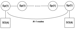
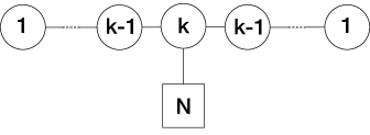
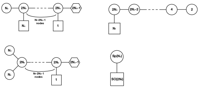
There are several tables below: Tab. 1 and Tab. 2 list star-shaped quivers and D-type quivers, Tab. 3 lists E-type and uneven star-shaped quivers111One of the quivers in the second table does not have any global symmetry; we thereby assume that its Coulomb branch is defined as a U(1)𝑈1U(1) quotient of the products of all its gauge groups., and Tab. 4 shows mirrors for Sp(Nc)𝑆𝑝subscript𝑁𝑐Sp(N_{c}) theories. Some notations: numbers inside circle nodes denote ranks of unitary gauge groups, numbers inside box nodes denote ranks of global symmetry groups, ‘A’ in rows four and five designate matter transforming in antisymmetric power of the fundamental representation of the group it is charged under.

We refer to mirror duals in these table as ‘A-model’ and ‘B-model’ which should be simply understood as a way of labeling the dual theories. We emphasize that this terminology is in no way connected to the 2d (homological) mirror symmetry.

Note that most of the mirror duals from the table below are already known.222The newly discovered “good” mirrors for double framed D^^𝐷\hat{D} quivers are displayed in Tab. 2. In this work we focus more on viewing the physics of these quivers through the prism of linear quivers and their mirrors rather than establishing new mirror pairs. As we show later in the text that for each quiver from the table there is a direct connection between its BPS protected quantities (parameter space of SUSY vacua and S3superscript𝑆3S^{3} partition function) and similar BPS objects for some linear quivers. We however admit that we do not possess an exhaustive classification of all quivers of this type (which can be obtained by gauging global symmetries of some linear quiver). It is a challenging task to provide such classification.

A-model B-model Location in the text
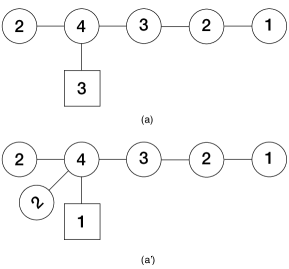
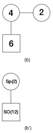
[Uncaptioned image] [Uncaptioned image] Sec. 4.1, Fig. 7
[Uncaptioned image] [Uncaptioned image] Sec. 4.3
[Uncaptioned image] [Uncaptioned image] Sec. 4.3, Fig. 15
[Uncaptioned image] [Uncaptioned image] Sec. 4.3, Fig. 16
[Uncaptioned image] [Uncaptioned image] Sec. 4.1, Fig. 22, (c)
[Uncaptioned image] [Uncaptioned image] Sec. 4.1, Fig. 22, (b)
Table 1: Summary table of star and D-shaped quivers and their mirrors.
A-model B-model Location in the text
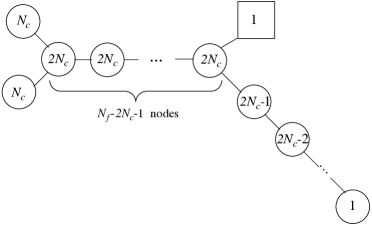
[Uncaptioned image] [Uncaptioned image] Sec. 4.4, Fig. 19
[Uncaptioned image] [Uncaptioned image] Sec. 4.4, Fig. 21
Table 2: Summary table of D-shaped quivers and their mirrors (continued).
A-model B-model Location in the text
[Uncaptioned image] [Uncaptioned image] Sec. 5, Fig. 27
[Uncaptioned image] [Uncaptioned image] Sec. 5, Fig. 28
[Uncaptioned image] [Uncaptioned image] Sec. 5, Fig. 30
Table 3: Summary table of star and E-shaped quivers and their mirrors.
A-model B-model Location in the text
[Uncaptioned image] [Uncaptioned image] Sec. 6, Fig. 35
Table 4: Sp(Nc)𝑆𝑝subscript𝑁𝑐Sp(N_{c}) gauge theory on the right with its mirror dual quiver.

2 𝒩=4𝒩4{\cal N}=4 Quivers, Mass Deformations and Mirror Symmetry

Our goal is to understand infrared physics of 𝒩=4𝒩4{\cal N}=4 and 𝒩=2𝒩superscript2{\cal N}=2^{\ast} three dimensional quiver theories which are formulated for quivers of every allowed shape. Recall that in three dimensions there is more freedom than, say, in four dimensions, where, in the subclass of balanced quivers, only (extended) ADE𝐴𝐷𝐸ADE-shaped quivers are allowed. Such quivers describe asymptotically conformal theories in the IR; integrating out matter multiplets one can easily obtain asymptotically free theories. However, in three dimensions the corresponding inequality for the linking numbers has the opposite sign. For example, 3d SQCD with gauge group Ncsubscript𝑁𝑐N_{c} and Nfsubscript𝑁𝑓N_{f} fundamental hypermultiples has to obey Nf2Ncsubscript𝑁𝑓2subscript𝑁𝑐N_{f}\geq 2N_{c} (so-called “good” quiver) in order to prevent the runaway of the vacua. Actually, theories with NcNf2Ncsubscript𝑁𝑐subscript𝑁𝑓2subscript𝑁𝑐N_{c}\leq N_{f}\leq 2N_{c} are also admissible, but their infrared physics is the same as the theory with NfNcsubscript𝑁𝑓subscript𝑁𝑐N_{f}-N_{c} colors and Nfsubscript𝑁𝑓N_{f} flavors. In what follows, unless otherwise specified we will assume that the stronger constraint Nf2Ncsubscript𝑁𝑓2subscript𝑁𝑐N_{f}\geq 2N_{c} is satisfied.

We start our analysis with linear ALsubscript𝐴𝐿A_{L} quiver theories (see Gaiotto:2008ak ; Gaiotto:2013bwa for details, here we provide only a minimal review) and then we shall develop an approach to study quivers of other shapes. The “goodness” condition for linear ALsubscript𝐴𝐿A_{L} quiver Fig. 1 with color labels Nisubscript𝑁𝑖N_{i} and flavor labels (framings) Misubscript𝑀𝑖M_{i} reads

Δi:=Ni+1+Ni1+Mi2Ni0.assignsubscriptΔ𝑖subscript𝑁𝑖1subscript𝑁𝑖1subscript𝑀𝑖2subscript𝑁𝑖0\Delta_{i}:=N_{i+1}+N_{i-1}+M_{i}-2N_{i}\geq 0\,. (1)

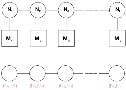
Several notations for quiver varieties are currently used in the literature. In Fig. 1 we list two of them which will be used in our paper interchangeably. These are so-called quanternionic representations of quivers. Each link corresponds to a hypermultiplet in (bi)fundamental representation of the gauge groups it connects. Complex quiver representations reflect each chiral multiplet separately.
Refer to caption
Figure 1: Two different notations of linear quiver ALsubscript𝐴𝐿A_{L} with labels (N1,M1)1(N2,M2)2(NL,ML)Lsubscriptsubscript𝑁1subscript𝑀11subscriptsubscript𝑁2subscript𝑀22subscriptsubscript𝑁𝐿subscript𝑀𝐿𝐿(N_{1},M_{1})_{1}(N_{2},M_{2})_{2}\dots(N_{L},M_{L})_{L}. Nisubscript𝑁𝑖N_{i} and Misubscript𝑀𝑖M_{i} are color and flavor labels of the i𝑖i-th node respectively.

A Nakajima quiver variety zbMATH00727829 is defined as a cotangent bundle to the space of the above quanternionic quiver representation followed by a hyper-Kähler quotient with respect to the gauge group action. In physics language this construction describes Higgs branches of quiver theories. In the above example of the U(Nc)𝑈subscript𝑁𝑐U(N_{c}) SQCD with Nfsubscript𝑁𝑓N_{f} fundamental hypermultiplets the quiver variety (Higgs branch) is isomorphic to the contingent bundle of the complex Grassmannian

Higgs=T(U(Nf)//U(Nc))=TGNf,Nc.\text{Higgs}=T^{\ast}(U(N_{f})//U(N_{c}))=T^{\ast}G_{N_{f},N_{c}}\,. (2)

Its quanternionic dimension is Nc(NfNc)subscript𝑁𝑐subscript𝑁𝑓subscript𝑁𝑐N_{c}(N_{f}-N_{c}).

In the infrared, moduli space of the theory has a Higgs branch and a Coulomb branch. On the Coulomb branch, one has an Abelian theory whose gauge group is the maximal torus of original gauge group of the quiver U(1)Ni𝑈superscript1subscript𝑁𝑖U(1)^{\sum N_{i}} while on the Higgs branch the gauge group is generically broken completely. The description of its moduli space depends on the amount of supersymmetry the theory possesses. In an 𝒩=4𝒩4{\cal N}=4 theory both the Higgs and the Coulomb branch are singular varieties and the type of singularity can be understood from the quiver itself. For example, it is well-known that the Higgs branch for affine ADE quivers has the corresponding ADE singularity. Since mirror symmetry exchanges Coulomb and Higgs branches, the Coulomb branch of the mirror dual of such quivers will also have the corresponding singularity.

For instance, consider a U(1)𝑈1U(1) gauge theory with M𝑀M electrons which is mirror dual to a AMsubscript𝐴𝑀A_{M} quiver. The Higgs branch of the latter is the Abelian orbifold 2/Msuperscript2subscript𝑀\mathbb{C}^{2}/\mathbb{Z}_{M} and therefore from mirror symmetry one expects the Coulomb branch of the former to be 2/Msuperscript2subscript𝑀\mathbb{C}^{2}/\mathbb{Z}_{M}. Using Hilbert Series analysis, one can readily check that this is indeed the case Cremonesi:2013lqa . The analysis is certainly more involved for non-Abelian gauge groups, but there is a canonical way to derive the representation content of the chiral ring on the Coulomb branchCremonesi:2013lqa . As we have just mentioned, Coulomb branches of such theories are singular and for Hilbert Series computation one does not need to consider the resolutions of these singularities. For S3superscript𝑆3S^{3} partition function computations, on the other hand, we require that these singularities are at least partially resolved. Therefore for each framing and for each node of the quiver one has to turn on resolution parameters (real masses and Fayet-Iliopoulos parameters respectively) compatible with 𝒩=4𝒩4{\cal N}=4 supersymmetry. On top of that, in order to make the parameter space of vacua of the theory (this is another variety we still need to define) nonsingular, we shall introduce another mass which will break the supersymmetry from 𝒩=4𝒩4{\cal N}=4 to 𝒩=2𝒩superscript2{\cal N}=2^{*} Gaiotto:2013bwa .

2.1 Brane Construction and Mirror Symmetry

Linear quiver theories can be conveniently formulated using brane constructions of Hanany-Witten type Hanany:1996ie . Hanany-Witten type brane setups have been extensively used in string theory and there are many detailed reviews in the literature; here we merely provide a prompt summary. The setup involves D3, NS5 and D5 branes which coincide in the worldvolume directions of the three-dimensional theory and are oriented in the complementary seven directions of Type IIB string theory such that the system preserves eight real supercharges- see the table below.

0 1 2 3 4 5 6 7 8 9
NS5 x x x x x x
D5 x x x x x x
D3 x x x x

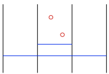
For example for quiver with labels (1,0)(2,2)(1,0)102210(1,0)(2,2)(1,0), which we will be using in the next section (see Fig. 7), we can draw brane diagram shown in Fig. 2.
Refer to caption
Figure 2: Brane construction for (1,0)(2,2)(1,0)102210(1,0)(2,2)(1,0) quiver. In this figure and later on, red ovals denote D5 branes, horizontal blue lines show D3 branes and vertical black lines designate NS5 branes. In a configuration where none of D3 branes end on D5 branes, the number of D3 branes contained in a given NS5 chamber gives the rank of the corresponding gauge group.

Let us now look at the field theory content in more details. Scalar fields parametrizing Higgs and Coulomb branches of the theory form a pair of SU(2)𝑆𝑈2SU(2) triplets. 𝒩=4𝒩4{\cal N}=4 SCFTs admit canonical mass deformations for flavor symmetries of Higgs and Coulomb branches. Therefore there are two types of mass deformations, also SU(2)𝑆𝑈2SU(2) triplets – real masses miAsubscriptsuperscript𝑚𝐴𝑖m^{A}_{i} on the Higgs branch of the theory and Fayet-Iliopoulos (FI) parameters taZsubscriptsuperscript𝑡𝑍𝑎t^{Z}_{a} on the Coulomb branch of the theory, here A,Z=1,2,3formulae-sequence𝐴𝑍123A,Z=1,2,3. The SU(2)𝑆𝑈2SU(2) symmetry is in fact geometrical, indeed the two symmetry algebras 𝔰𝔲(2)𝔰𝔬(3)similar-to𝔰𝔲2𝔰𝔬3\mathfrak{su}(2)\sim\mathfrak{so}(3) are represented via rotations of 456456456 directions for the Higgs branch R-symmetry and 789789789 directions for the Coulomb branch R-symmetry. For each i𝑖i the values of miA,A=4,5,6formulae-sequencesuperscriptsubscript𝑚𝑖𝐴𝐴456m_{i}^{A},\,A=4,5,6 and taZ,Z=7,8,9formulae-sequencesuperscriptsubscript𝑡𝑎𝑍𝑍789t_{a}^{Z},\,Z=7,8,9 give the coordinates of i𝑖ith D5 brane inside 4563subscriptsuperscript3456\mathbb{R}^{3}_{456} and i𝑖ith NS5 brane inside 7893subscriptsuperscript3789\mathbb{R}^{3}_{789}. Because of the translational symmetry of 3superscript3\mathbb{R}^{3} all coordinates should be counted modulo the overall shift. In fact, only the differences taZta1Zsubscriptsuperscript𝑡𝑍𝑎subscriptsuperscript𝑡𝑍𝑎1t^{Z}_{a}-t^{Z}_{a-1} have actual physical meaning as FI parameters for the corresponding gauge groups in the linear quiver. Sometimes it is convenient to impose a center of mass constraint on them as well as on the masses for each gauge node of the quiver but we shall refrain from doing so in this paper. It will turn out, somewhat surprisingly, that keeping all the mass deformations unconstrained has some advantage when one works with S-duality and mirror symmetry.

The mirror symmetry in three dimensions can be easily understood via S-duality of the above brane construction. Under S-duality NS5 branes turn into D5 branes and vice versa, D3 branes remain self dual. To read off the dual gauge theory from the S-dual brane system, one needs to move the D5 and NS5 branes appropriately with possible creation/annihilation of D3 branes required to keep the linking numbers of the individual 5-branes invariant Hanany:1996ie ; Gaiotto:2008ak . Because Dirichlet and Neveu-Schwarz branes are interchanged Higgs and Coulomb branches are to be swapped together with the SU(2)𝑆𝑈2SU(2) R-symmetries. In the following sections of the paper we will be using various examples of mirror dual quiver theories, but for now let us consider the mirror for the theory depicted in Fig. 2. It is an A1subscript𝐴1A_{1} quiver with labels (2,4)24(2,4) or 3d U(2)𝑈2U(2) SQCD with four fundamental hypermultiplets. Indeed, if we switch the NS5 and D5 branes in Fig. 2 and move NS5 branes to the boundaries of the picture, invariance of linking numbers for various 5-branes will dictate that the four D5 branes lie inside the NS5 chamber and two D3 branes end on these NS5 branes. This is clearly the Type IIB description for the A1subscript𝐴1A_{1} quiver (2,4)24(2,4).

Note that we can easily generalize the prescription of obtaining mirror duals to theories given by affine A^Nsubscript^𝐴𝑁\hat{A}_{N} quivers. Circular D3 branes which wrap around all the NS5 branes are selfdual, so it is straightforward to read off the data of the mirror quiver. Later in Sec. 4.4 we shall consider a framed A^3subscript^𝐴3\hat{A}_{3} quiver and its mirror.

2.2 Parameter Space of Vacua for ALsubscript𝐴𝐿A_{L} Quivers

We need to introduce one more ingredient – the space of mass parameters of supersymmetric vacua {\cal L} for quiver gauge theories in question. However, in order to define {\cal L} we need to deform the setup twofold (see Gaiotto:2013bwa for details): First, we compactify the theory on 2×S1superscript2superscript𝑆1\mathbb{R}^{2}\times S^{1}, and, second, we turn on another mass deformation which breaks the supersymmetry down to 𝒩=2𝒩2{\cal N}=2. Both modifications are absolutely necessary in order to transform {\cal L} into a complex symplectic manifold with symplectic form

Ω=idpmidmi+adptadta,Ωsubscript𝑖𝑑superscriptsubscript𝑝𝑚𝑖𝑑subscript𝑚𝑖subscript𝑎𝑑superscriptsubscript𝑝𝑡𝑎𝑑subscript𝑡𝑎\Omega=\sum_{i}dp_{m}^{i}\wedge dm_{i}+\sum_{a}dp_{t}^{a}\wedge dt_{a}\,, (3)

where the conjugate momenta pt,msubscript𝑝𝑡𝑚p_{t,m} to (now complexified) coordinates misubscript𝑚𝑖m_{i} and tasubscript𝑡𝑎t_{a} are defined through the following generating function

pmi=𝒲(s,m,t)mi,pta=𝒲(s,m,t)ta.formulae-sequencesuperscriptsubscript𝑝𝑚𝑖𝒲𝑠𝑚𝑡subscript𝑚𝑖superscriptsubscript𝑝𝑡𝑎𝒲𝑠𝑚𝑡subscript𝑡𝑎p_{m}^{i}=\frac{\partial{\cal W}(s,m,t)}{\partial m_{i}}\,,\quad p_{t}^{a}=\frac{\partial{\cal W}(s,m,t)}{\partial t_{a}}\,. (4)

The generating function 𝒲(s,m,t)𝒲𝑠𝑚𝑡{\cal W}(s,m,t) is nothing but the twisted effective superpotential which describes the massive vacua of the 𝒩=2𝒩2{\cal N}=2 theory. The twisted superpotential can be derived straightforwardly from the UV description of the theory by integrating out all chiral multiplets Nekrasov:2009uh . As is explained in Gaiotto:2013bwa , 𝒲𝒲{\cal W} serves as a generating function on the parameter space of vacua, which represents itself as a symplectic Lagrangian submanifold {\cal L}\subset{\cal M} inside the complex vector space of all coordinates (masses and FI terms) and the corresponding conjugate momenta.

The 𝒩=2𝒩superscript2{\cal N}=2^{*} deformation is implemented by the canonical embedding of the 𝒩=2𝒩2{\cal N}=2 supersymmetry algebra inside the 𝒩=4𝒩4{\cal N}=4 supersymmetry algebra, namely, the U(1)𝑈1U(1) R-symmetry generator of the 𝒩=2𝒩2{\cal N}=2 subalgebra is given by the sum of two Cartan generators of SU(2)Higgs×SU(2)Coulomb𝑆𝑈subscript2Higgs𝑆𝑈subscript2CoulombSU(2)_{\text{Higgs}}\times SU(2)_{\text{Coulomb}} 𝒩=4𝒩4{\cal N}=4 algebra R-symmetry 𝔧R=𝔧Higgs3+𝔧Coulomb3subscript𝔧𝑅subscriptsuperscript𝔧3Higgssubscriptsuperscript𝔧3Coulomb\mathfrak{j}_{R}=\mathfrak{j}^{3}_{\text{Higgs}}+\mathfrak{j}^{3}_{\text{Coulomb}}. The orthogonal Cartan generator 𝔧ϵ=𝔧Higgs3𝔧Coulomb3subscript𝔧italic-ϵsubscriptsuperscript𝔧3Higgssubscriptsuperscript𝔧3Coulomb\mathfrak{j}_{\epsilon}=\mathfrak{j}^{3}_{\text{Higgs}}-\mathfrak{j}^{3}_{\text{Coulomb}} commutes with the 𝒩=2𝒩2{\cal N}=2 subalgebra and generates U(1)ϵ𝑈subscript1italic-ϵU(1)_{\epsilon} flavor symmetry with ϵitalic-ϵ\epsilon being the corresponding twisted mass.

Finally, the circle compactification provides us with complex mass parameters which are obtained by combining real masses and FI terms with the corresponding flavor Wilson lines. Due to the periodicity along the compact direction it is convenient to replace tuple (mi,ta,ϵ)subscript𝑚𝑖subscript𝑡𝑎italic-ϵ(m_{i},t_{a},\epsilon) by its trigonometric version

μi=e2πRmi,τa=e2πRta,η=e4πRϵ,formulae-sequencesubscript𝜇𝑖superscript𝑒2𝜋𝑅subscript𝑚𝑖formulae-sequencesubscript𝜏𝑎superscript𝑒2𝜋𝑅subscript𝑡𝑎𝜂superscript𝑒4𝜋𝑅italic-ϵ\mu_{i}=e^{2\pi Rm_{i}}\,,\quad\tau_{a}=e^{2\pi Rt_{a}}\,,\quad\eta=e^{4\pi R\epsilon}\,, (5)

where the numerical factors in the exponential are conventions. Analogously to (4) we introduce exponentiated momenta

pμi=e2πRpmi,pτa=e2πRpta,pη=e4πR𝒲ϵ,formulae-sequencesuperscriptsubscript𝑝𝜇𝑖superscript𝑒2𝜋𝑅superscriptsubscript𝑝𝑚𝑖formulae-sequencesuperscriptsubscript𝑝𝜏𝑎superscript𝑒2𝜋𝑅superscriptsubscript𝑝𝑡𝑎subscript𝑝𝜂superscript𝑒4𝜋𝑅𝒲italic-ϵp_{\mu}^{i}=e^{2\pi Rp_{m}^{i}}\,,\quad p_{\tau}^{a}=e^{2\pi Rp_{t}^{a}}\,,\quad p_{\eta}=e^{4\pi R\frac{\partial{\cal W}}{\partial\epsilon}}\,, (6)

where in the end we have introduced the momentum conjugate to ϵitalic-ϵ\epsilon, which can also be treated an independent coordinate.

The twisted superpotential 𝒲(s,m,t,ϵ)𝒲𝑠𝑚𝑡italic-ϵ{\cal W}(s,m,t,\epsilon) is to be minimized with respect to the adjoint scalar s𝑠s of the 𝒩=2𝒩2\mathcal{N}=2, 3d vector superfield, which can also be exponentiated

σi=e2πRsi.subscript𝜎𝑖superscript𝑒2𝜋𝑅subscript𝑠𝑖\sigma_{i}=e^{2\pi Rs_{i}}\,. (7)

In the same symplectic fashion we introduce canonical momenta which are conjugate to s𝑠s The condition for supersymmetric vacua is thus precisely the extrema of 𝒲𝒲{\cal W}

pσi:=exp2πR𝒲si=1.assignsuperscriptsubscript𝑝𝜎𝑖2𝜋𝑅𝒲subscript𝑠𝑖1p_{\sigma}^{i}:=\exp 2\pi R\frac{\partial{\cal W}}{\partial s_{i}}=1\,. (8)

Therefore algebraically vacua moduli space {\cal L} is a Lagrangian submanifold in {\cal M} given by specifying the conjugate momenta to the full set of variables: s,mi,ta,ϵ𝑠subscript𝑚𝑖superscript𝑡𝑎italic-ϵs,m_{i},t^{a},\epsilon.

The mirror symmetry in three dimensions interchanges FI terms and masses, hence it should also interchange the corresponding conjugate momenta. In particular it implies that pμisuperscriptsubscript𝑝𝜇𝑖p_{\mu}^{i} of one model should coincide with pτasuperscriptsubscript𝑝𝜏𝑎p_{\tau}^{a} of the mirror dual model up to (possibly) some identifications of the mass deformations on both sides. On top of that the mirror symmetry flips the sign of ϵitalic-ϵ\epsilon since it negates the action of the U(1)ϵ𝑈subscript1italic-ϵU(1)_{\epsilon} generator we introduced above.

2.3 The Partition Function on S3superscript𝑆3S^{3}

Localization methods have emerged as a powerful toolbox for computing various observables exactly in QFTs with enough supersymmetryPestun:2007rz ; Kapustin:2009kz ; Hama:2011ea ; Festuccia:2011ws . The study of localization for 𝒩2𝒩2{\cal N}\geq 2 quiver gauge theories on S3superscript𝑆3S^{3} was initiated in Kapustin:2009kz and in recent years such computations have been carried out extensively for various three-manifolds including the squashed sphere Sb3subscriptsuperscript𝑆3𝑏S^{3}_{b} Hama:2011ea . In the b0𝑏0b\to 0 limit the squashed sphere partition function simplifies dramatically, namely it becomes the exponential of the twisted effective superpotential 𝒵Sb3ei𝒲similar-tosubscript𝒵subscriptsuperscript𝑆3𝑏superscript𝑒𝑖𝒲\mathcal{Z}_{S^{3}_{b}}\sim e^{-i{\cal W}}. Therefore we recover the classical parameter space of the mass deformations {\cal L} in this limit. On the other hand, b1similar-to𝑏1b\sim 1 value corresponds to an intrinsic quantum regime333The radius of the sphere coincides with b𝑏b in this limit.

The computations of the squashed sphere partition function are slightly cumbersome due to the presence of special functions constructed from double infinite products. However, those functions reduce to exponentials for the round sphere when b=1𝑏1b=1. The partition function on round sphere is therefore a particularly convenient object for studying dualities in 3d quiver gauge theories. Explicit computations of S3superscript𝑆3S^{3} partition functions as tools to check three dimensional mirror symmetry for 𝒩=4𝒩4{\cal N}=4 quiver gauge theories was discussed in Kapustin:2010xq . This approach was also taken in Dey:2011pt ; Dey:2013nf where mirror symmetry for a large class of affine D𝐷D-type quivers was discussed.

Given an 𝒩=4𝒩4{\cal N}=4 quiver gauge theory, the rules for writing down the S3superscript𝑆3S^{3} partition function may be summarized in the following fashion. Localization ensures that the partition function of the theory reduces to a matrix integral over the Cartan of the gauge group. Since S3superscript𝑆3S^{3} does not have any instantons, any such partition function may be schematically represented as

𝒵=dks|𝒲|αα(s)expScl[s]𝒵1-loop[s],𝒵superscript𝑑𝑘𝑠𝒲subscriptproduct𝛼𝛼𝑠subscript𝑆cldelimited-[]𝑠subscript𝒵1-loopdelimited-[]𝑠{\cal Z}=\int\frac{d^{k}s}{|\mathcal{W}|}\prod_{\alpha}\alpha(s)\exp{S_{\text{cl}}[s]}\,{\cal Z}_{\text{1-loop}}[s]\,, (9)

where s𝑠s is the real adjoint scalar that sits inside a 3d 𝒩=2𝒩2\mathcal{N}=2 vector multiplet. One can use a constant gauge transformation to make s𝑠s lie in the Cartan subalgebra of the gauge group. In the above formula αα(s)subscriptproduct𝛼𝛼𝑠\prod_{\alpha}\alpha(s) is the Vandermonte determinant where the product is over all roots of the gauge group. This factor appears in the measure as a result of gauge fixing the matrix model such that s𝑠s lies in the Cartan of the gauge group. |𝒲|𝒲|\mathcal{W}| represents the order of the Weyl group - the 1|𝒲|1𝒲\frac{1}{|\mathcal{W}|} factor is needed to account for the residual gauge symmetry after s𝑠s is gauge-fixed to lie in the Cartan subalgebra.

The contribution of vectors and hypers in the 𝒩=4𝒩4{\cal N}=4 theory to the above partition are as follows. For every U(1)𝑈1U(1) factor in the gauge group, one obtains the following classical contribution

SclFI=2πiηTr(s),subscriptsuperscript𝑆FIcl2𝜋𝑖𝜂Tr𝑠S^{\text{FI}}_{\text{cl}}=2\pi i\eta\,\text{Tr}(s)\,, (10)

where η𝜂\eta is a FI parameter. Each 𝒩=4𝒩4\mathcal{N}=4 vector multiplet contributes with

Z1-loopv=αsinh2πα(s)πα(s),subscriptsuperscript𝑍𝑣1-loopsubscriptproduct𝛼superscript2𝜋𝛼𝑠𝜋𝛼𝑠Z^{v}_{\text{1-loop}}=\prod_{\alpha}\frac{\sinh^{2}{\pi\alpha(s)}}{\pi\alpha(s)}\,, (11)

where the product extends over all the roots of the Lie algebra of G. In fact, this is precisely the contribution of an 𝒩=2𝒩2\mathcal{N}=2 vector multiplet since contribution of the adjoint chiral which is part of the 𝒩=4𝒩4\mathcal{N}=4 vector multiplet is trivial Kapustin:2010xq .

Finally, each 𝒩=4𝒩4\mathcal{N}=4 hypermultiplet contributes with

𝒵1-looph=ρ1coshπρ(s+m),subscriptsuperscript𝒵1-loopsubscriptproduct𝜌1𝜋𝜌𝑠𝑚{\cal Z}^{h}_{\text{1-loop}}=\prod_{\rho}\frac{1}{\cosh{\pi\rho(s+m)}}\,, (12)

where the product extends over all the weights of the representation R of the gauge group G and m𝑚m is a real mass parameter.

Note that the Vandermonte factor in the measure exactly cancels with the denominator of the 1-loop contribution of the vector multiplet for each factor in the gauge group and we can therefore ignore this contribution in the matrix integral.

Now let us illustrate how S3superscript𝑆3S^{3} partition function may be useful in studying mirror symmetry of 𝒩=4𝒩4\mathcal{N}=4 quiver gauge theories. Consider the linear quiver pair which we have already discussed in this section: the A-model quiver with labels (1,0)(2,2)(1,0)102210(1,0)(2,2)(1,0) (see Fig. 2) and its mirror, the B-model which has labels (2,4)24(2,4). The A-model partition function is given by

𝒵A=α=12dsαd2s02!α=12e2πisαηαi=12e2πis0iη0sinh2π(s01s02)i=12coshπ(s1s0i)a=12coshπ(s0i+ma)coshπ(s2s0i)=e2πim1(t1+t2)e2πim2(t3+t4)12sinhπ(t1t2)sinhπ(t3t4)sinh2π(m1m2)×[(e2πit4(m1m2)e2πit1(m1m2))(e2πit3(m1m2)e2πit2(m1m2))sinhπ(t2t3)sinhπ(t1t4)(e2πit3(m1m2)e2πit1(m1m2))(e2πit4(m1m2)e2πit2(m1m2))sinhπ(t1t3)sinhπ(t2t4)],subscript𝒵𝐴subscriptsuperscriptproduct2𝛼1𝑑subscript𝑠𝛼superscript𝑑2subscript𝑠02subscriptsuperscriptproduct2𝛼1superscript𝑒2𝜋𝑖subscript𝑠𝛼subscript𝜂𝛼subscriptsuperscriptproduct2𝑖1superscript𝑒2𝜋𝑖subscriptsuperscript𝑠𝑖0subscript𝜂0superscript2𝜋subscriptsuperscript𝑠10subscriptsuperscript𝑠20subscriptsuperscriptproduct2𝑖1𝜋subscript𝑠1subscriptsuperscript𝑠𝑖0subscriptsuperscriptproduct2𝑎1𝜋subscriptsuperscript𝑠𝑖0subscript𝑚𝑎𝜋subscript𝑠2subscriptsuperscript𝑠𝑖0superscript𝑒2𝜋𝑖subscript𝑚1subscript𝑡1subscript𝑡2superscript𝑒2𝜋𝑖subscript𝑚2subscript𝑡3subscript𝑡412𝜋subscript𝑡1subscript𝑡2𝜋subscript𝑡3subscript𝑡4superscript2𝜋subscript𝑚1subscript𝑚2delimited-[]superscript𝑒2𝜋𝑖subscript𝑡4subscript𝑚1subscript𝑚2superscript𝑒2𝜋𝑖subscript𝑡1subscript𝑚1subscript𝑚2superscript𝑒2𝜋𝑖subscript𝑡3subscript𝑚1subscript𝑚2superscript𝑒2𝜋𝑖subscript𝑡2subscript𝑚1subscript𝑚2𝜋subscript𝑡2subscript𝑡3𝜋subscript𝑡1subscript𝑡4superscript𝑒2𝜋𝑖subscript𝑡3subscript𝑚1subscript𝑚2superscript𝑒2𝜋𝑖subscript𝑡1subscript𝑚1subscript𝑚2superscript𝑒2𝜋𝑖subscript𝑡4subscript𝑚1subscript𝑚2superscript𝑒2𝜋𝑖subscript𝑡2subscript𝑚1subscript𝑚2𝜋subscript𝑡1subscript𝑡3𝜋subscript𝑡2subscript𝑡4\begin{split}&{\cal Z}_{A}=\int\prod^{2}_{\alpha=1}ds_{\alpha}\frac{d^{2}s_{0}}{2!}\frac{\prod^{2}_{\alpha=1}e^{2\pi is_{\alpha}\eta_{\alpha}}\prod^{2}_{i=1}e^{2\pi is^{i}_{0}\eta_{0}}\sinh^{2}{\pi(s^{1}_{0}-s^{2}_{0})}}{\prod^{2}_{i=1}\cosh{\pi(s_{1}-s^{i}_{0})}\prod^{2}_{a=1}\cosh{\pi(s^{i}_{0}+m_{a})}\cosh{\pi(s_{2}-s^{i}_{0})}}\\ &=e^{-2\pi im_{1}(t_{1}+t_{2})}e^{2\pi im_{2}(t_{3}+t_{4})}\frac{1}{2\sinh{\pi(t_{1}-t_{2})}\sinh{\pi(t_{3}-t_{4})}\sinh^{2}{\pi(m_{1}-m_{2})}}\\ \times&\Big{[}\frac{(e^{2\pi it_{4}(m_{1}-m_{2})}-e^{2\pi it_{1}(m_{1}-m_{2})})(e^{2\pi it_{3}(m_{1}-m_{2})}-e^{2\pi it_{2}(m_{1}-m_{2})})}{\sinh{\pi(t_{2}-t_{3})}\sinh{\pi(t_{1}-t_{4})}}\\ &-\frac{(e^{2\pi it_{3}(m_{1}-m_{2})}-e^{2\pi it_{1}(m_{1}-m_{2})})(e^{2\pi it_{4}(m_{1}-m_{2})}-e^{2\pi it_{2}(m_{1}-m_{2})})}{\sinh{\pi(t_{1}-t_{3})}\sinh{\pi(t_{2}-t_{4})}}\Big{]}\,,\end{split} (13)

where m1subscript𝑚1m_{1} and m4subscript𝑚4m_{4} are the masses of the fundamental hypermultiplets in the middle node. We have also defined η1=t1t2,η0=t2t3,η2=t3t4formulae-sequencesubscript𝜂1subscript𝑡1subscript𝑡2formulae-sequencesubscript𝜂0subscript𝑡2subscript𝑡3subscript𝜂2subscript𝑡3subscript𝑡4\eta_{1}=t_{1}-t_{2},\eta_{0}=t_{2}-t_{3},\eta_{2}=t_{3}-t_{4} which are the Abelian coupling constants for the three gauge groups in the quiver.

The partition function of the B-model (2,4)24(2,4) is

𝒵B=d2s2!i=12e2πisi(t~1t~2)sinh2π(s1s2)i=12a=14coshπ(si+Ma)=12sinhπ(M1M2)sinhπ(M3M4)sinh2π(t~1t~2)×[(e2πiM1(t~1t~2)e2πiM4(t~1t~2))(e2πiM2(t~1t~2)e2πiM3(t~1t~2))sinhπ(M1M4)sinhπ(M2M3)(e2πiM1(t~1t~2)e2πiM3(t~1t~2))(e2πiM2(t~1t~2)e2πiM4(t~1t~2))sinhπ(M1M3)sinhπ(M2M4)].subscript𝒵𝐵superscript𝑑2𝑠2subscriptsuperscriptproduct2𝑖1superscript𝑒2𝜋𝑖superscript𝑠𝑖subscript~𝑡1subscript~𝑡2superscript2𝜋superscript𝑠1superscript𝑠2subscriptsuperscriptproduct2𝑖1subscriptsuperscriptproduct4𝑎1𝜋superscript𝑠𝑖subscript𝑀𝑎12𝜋subscript𝑀1subscript𝑀2𝜋subscript𝑀3subscript𝑀4superscript2𝜋subscript~𝑡1subscript~𝑡2delimited-[]superscript𝑒2𝜋𝑖subscript𝑀1subscript~𝑡1subscript~𝑡2superscript𝑒2𝜋𝑖subscript𝑀4subscript~𝑡1subscript~𝑡2superscript𝑒2𝜋𝑖subscript𝑀2subscript~𝑡1subscript~𝑡2superscript𝑒2𝜋𝑖subscript𝑀3subscript~𝑡1subscript~𝑡2𝜋subscript𝑀1subscript𝑀4𝜋subscript𝑀2subscript𝑀3superscript𝑒2𝜋𝑖subscript𝑀1subscript~𝑡1subscript~𝑡2superscript𝑒2𝜋𝑖subscript𝑀3subscript~𝑡1subscript~𝑡2superscript𝑒2𝜋𝑖subscript𝑀2subscript~𝑡1subscript~𝑡2superscript𝑒2𝜋𝑖subscript𝑀4subscript~𝑡1subscript~𝑡2𝜋subscript𝑀1subscript𝑀3𝜋subscript𝑀2subscript𝑀4\begin{split}&{\cal Z}_{B}=\int\frac{d^{2}s}{2!}\frac{\prod^{2}_{i=1}e^{2\pi is^{i}(\widetilde{t}_{1}-\widetilde{t}_{2})}\sinh^{2}{\pi(s^{1}-s^{2})}}{\prod^{2}_{i=1}\prod^{4}_{a=1}\cosh{\pi(s^{i}+M_{a})}}\\ &=\frac{1}{2\sinh{\pi(M_{1}-M_{2})}\sinh{\pi(M_{3}-M_{4})}\sinh^{2}{\pi(\widetilde{t}_{1}-\widetilde{t}_{2})}}\\ &\times\Big{[}\frac{(e^{2\pi iM_{1}(\widetilde{t}_{1}-\widetilde{t}_{2})}-e^{2\pi iM_{4}(\widetilde{t}_{1}-\widetilde{t}_{2})})(e^{2\pi iM_{2}(\widetilde{t}_{1}-\widetilde{t}_{2})}-e^{2\pi iM_{3}(\widetilde{t}_{1}-\widetilde{t}_{2})})}{\sinh{\pi(M_{1}-M_{4})}\sinh{\pi(M_{2}-M_{3})}}\\ &-\frac{(e^{2\pi iM_{1}(\widetilde{t}_{1}-\widetilde{t}_{2})}-e^{2\pi iM_{3}(\widetilde{t}_{1}-\widetilde{t}_{2})})(e^{2\pi iM_{2}(\widetilde{t}_{1}-\widetilde{t}_{2})}-e^{2\pi iM_{4}(\widetilde{t}_{1}-\widetilde{t}_{2})})}{\sinh{\pi(M_{1}-M_{3})}\sinh{\pi(M_{2}-M_{4})}}\Big{]}\,.\end{split} (14)

For convenience we impose the following constraints on mass parameters and FI parameters: t~2+t~1=0subscript~𝑡2subscript~𝑡10\widetilde{t}_{2}+\widetilde{t}_{1}=0 and M1+M2+M3+M4=0subscript𝑀1subscript𝑀2subscript𝑀3subscript𝑀40M_{1}+M_{2}+M_{3}+M_{4}=0.

From the formulae for 𝒵Asubscript𝒵𝐴{\cal Z}_{A} and 𝒵Bsubscript𝒵𝐵{\cal Z}_{B}, it is evident that they are equivalent under the mirror map

tiMi,mat~a,subscript𝑡𝑖subscript𝑀𝑖subscript𝑚𝑎subscript~𝑡𝑎t_{i}\leftrightarrow M_{i}\,,\quad m_{a}\leftrightarrow\widetilde{t}_{a}\,, (15)

up to a phase factor e2πim1(t1+t2)e2πim2(t3+t4)superscript𝑒2𝜋𝑖subscript𝑚1subscript𝑡1subscript𝑡2superscript𝑒2𝜋𝑖subscript𝑚2subscript𝑡3subscript𝑡4e^{2\pi im_{1}(t_{1}+t_{2})}e^{-2\pi im_{2}(t_{3}+t_{4})} which vanishes when one imposes the constraints m1+m2=0,t1+t2+t3+t4=0formulae-sequencesubscript𝑚1subscript𝑚20subscript𝑡1subscript𝑡2subscript𝑡3subscript𝑡40m_{1}+m_{2}=0,\;t_{1}+t_{2}+t_{3}+t_{4}=0.

In the following sections, we shall make extensive use of the S3superscript𝑆3S^{3} partition function to obtain various quiver gauge theories from linear quiver pairs using the technique of abelian/non-abelian gauging.

2.4 The Hilbert Series of the Coulomb Branch

In this section we review a general formula for the Hilbert series of the Coulomb branch of a 3d3𝑑3d 𝒩=4𝒩4\mathcal{N}=4 theory discussed in Cremonesi:2013lqa .

It is convenient to use the 3d3𝑑3d 𝒩=2𝒩2{\cal N}=2 formalism, in which the 𝒩=4𝒩4{\cal N}=4 vector multiplet decomposes into a 𝒩=2𝒩2{\cal N}=2 vector multiplet and a chiral multiplet ΦΦ\Phi in the adjoint representation of the gauge group. On a generic point of the Coulomb moduli space, the triplet of scalars in the 𝒩=4𝒩4{\cal N}=4 vector multiplets acquires a vacuum expectation value, and the gauge fields that remain massless are abelian and can be dualized to scalar fields. The classical Coulomb branch is parametrized by the collection of such massless scalar fields. The Coulomb branch, however, receives many quantum corrections. The asymptotic hyperkähler metric in the weak coupling region of the Coulomb branch can be computed at one loop. Yet this method does not provide a suitable description for the strongly coupled region.

It is shown in Borokhov:2002ib that there is a description of the quantum Coulomb branch that bypasses the dualization of free abelian vector multiplets. This realization involves ’t Hooft monopole operators, which are local disorder operators that can be defined directly in the infrared CFT. The magnetic charges 𝒎𝒎\bm{m} of the monopole operators are labelled by the weight lattice ΓGsubscriptsuperscriptΓsuperscript𝐺\Gamma^{*}_{G^{\vee}} of the GNO (Langlands) dual gauge group Gsuperscript𝐺G^{\vee} Goddard:1976qe . The GNO monopole charges 𝒎𝒎\bm{m} breaks the gauge group G𝐺G to a residual gauge group H𝒎subscript𝐻𝒎H_{\bm{m}}, which is the commutant of 𝒎𝒎\bm{m} inside G𝐺G. The components of the complex scalar ϕitalic-ϕ\phi that are moduli of the BPS monopole configuration reside in the Lie algebra of the group H𝒎subscript𝐻𝒎H_{\bm{m}} and are left unbroken by the monopole flux Cremonesi:2013lqa . The monopoles can be dressed with the scalar components ϕitalic-ϕ\phi of the chiral multiplet ΦΦ\Phi that preserves some amount of supersymmetry. The residual gauge symmetry in the monopole background contains continuous part H𝒎subscript𝐻𝒎H_{\bm{m}} and a discrete part, namely Weyl group WGsubscript𝑊superscript𝐺W_{G^{\vee}} of Gsuperscript𝐺G^{\vee}; they act on 𝒎𝒎\bm{m} and ϕitalic-ϕ\phi. The gauge invariant operators are labelled by 𝒎ΓG/WG𝒎subscriptsuperscriptΓsuperscript𝐺subscript𝑊superscript𝐺\bm{m}\in\Gamma^{*}_{G^{\vee}}/W_{G^{\vee}}, i.e.  a Weyl chamber of weight lattice ΓGsubscriptsuperscriptΓsuperscript𝐺\Gamma^{*}_{G^{\vee}}. Such operators are dressed by all possible products of ϕitalic-ϕ\phi which are invariant under the action of the residual group H𝒎subscript𝐻𝒎H_{\bm{m}}.

The Hilbert series is the generating function of the chiral ring that counts gauge invariant BPS operators parametrizing the Coulomb branch, graded according to their dimension and quantum numbers under global symmetries. From the above discussion, the general formula for the Coulomb branch Hilbert series reads

HG(t,z)=𝒎ΓG/WGtΔ(𝒎)PG(t,𝒎)zJ(𝒎),subscript𝐻𝐺𝑡𝑧subscript𝒎subscriptsuperscriptΓsuperscript𝐺subscript𝑊superscript𝐺superscript𝑡Δ𝒎subscript𝑃𝐺𝑡𝒎superscript𝑧𝐽𝒎\displaystyle H_{G}(t,z)=\sum_{\bm{m}\,\in\,\Gamma^{*}_{G^{\vee}}/W_{G^{\vee}}}t^{\Delta(\bm{m})}P_{G}(t,\bm{m})z^{J(\bm{m})}\;, (16)

where the notation is explained as follows:

  • The sum is taken over a Weyl Chamber of the weight lattice ΓGsubscriptsuperscriptΓsuperscript𝐺\Gamma^{*}_{G^{\vee}},

  • The function PG(t,m)subscript𝑃𝐺𝑡𝑚P_{G}(t,m) counts Casimir gauge invariants of the residual gauge group H𝒎subscript𝐻𝒎H_{\bm{m}} made with the adjoint ϕitalic-ϕ\phi, according to their dimension; it is given by

    PG(t;𝒎)=i=1r11tdi(𝒎),subscript𝑃𝐺𝑡𝒎superscriptsubscriptproduct𝑖1𝑟11superscript𝑡subscript𝑑𝑖𝒎\displaystyle P_{G}(t;\bm{m})=\prod_{i=1}^{r}\frac{1}{1-t^{d_{i}(\bm{m})}}\;, (17)

    where di(𝒎)subscript𝑑𝑖𝒎d_{i}(\bm{m}), i=1,,rankH𝒎𝑖1ranksubscript𝐻𝒎i=1,\dots,{\rm rank}\;H_{\bm{m}} are the degrees of the Casimir invariants of the residual gauge group H𝒎subscript𝐻𝒎H_{\bm{m}} left unbroken by the GNO magnetic flux 𝒎𝒎\bm{m}.

  • The factor tΔ(m)superscript𝑡Δ𝑚t^{\Delta(m)} takes into account quantum dimensions of monopole operators which is given by Borokhov:2002cg ; Gaiotto:2008ak ; Benna:2009xd ; Bashkirov:2010kz

    Δ(𝒎)=𝜶Δ+(G)|α(𝒎)|+12i=1n𝝆iRi|𝝆i(𝒎)|,Δ𝒎subscript𝜶subscriptΔ𝐺𝛼𝒎12superscriptsubscript𝑖1𝑛subscriptsubscript𝝆𝑖subscript𝑅𝑖subscript𝝆𝑖𝒎\displaystyle\Delta(\bm{m})=-\sum_{\bm{\alpha}\in\Delta_{+}(G)}|\alpha(\bm{m})|+\frac{1}{2}\sum_{i=1}^{n}\sum_{\bm{\rho}_{i}\in R_{i}}|\bm{\rho}_{i}(\bm{m})|\;, (18)

    where the first sum over positive roots 𝜶Δ+(G)𝜶subscriptΔ𝐺\bm{\alpha}\in\Delta_{+}(G) of G𝐺G is the contribution of 𝒩=4𝒩4\mathcal{N}=4 vector multiplets and the second sum over the weights 𝝆isubscript𝝆𝑖\bm{\rho}_{i} of the matter field representation Risubscript𝑅𝑖R_{i} under the gauge group is the contribution of the i𝑖i-th 𝒩=4𝒩4\mathcal{N}=4 hypermultiplet.

  • For a non-simple connected group G𝐺G, there is a non-trivial topological symmetry under which the monopole operators are charged. J(𝒎)𝐽𝒎J(\bm{m}) denotes the topological charge of the monopole operator of GNO charges 𝒎𝒎\bm{m}, and z𝑧z is the fugacity associated with the topological charge.

We refer to (16) as the monopole formula of the Coulomb branch Hilbert series.

3 Gauging Quivers: A Basic Example

Let us describe a simple example which illustrates the main idea of the gauging method. In this section we shall only discuss Abelian gauging by which we shall mean gauging a single, or several U(1) factors. In later sections we shall address non-Abelian gauging, which will result in a nontrivial deformation of the Coulomb branch of the mirror model.

3.1 Parameter Space Approach

In this work we shall be repeatedly using the embedding of parameter spaces of various quiver gauge theories {\cal L} into larger parameter spaces of some linear ALsubscript𝐴𝐿A_{L} quivers whose mirrors can be easily constructed. Using the results of Gaiotto:2013bwa we can approach the desired parameter space by taking some singular limit of the ALsubscript𝐴𝐿A_{L} mirror pair. Each 𝒩=2𝒩2\mathcal{N}=2 ALsubscript𝐴𝐿A_{L} quiver theory has a fairly large parameter space of masses μi(I)subscriptsuperscript𝜇𝐼𝑖\mu^{(I)}_{i} (I𝐼I corresponds to I𝐼I-th gauge node) and FI couplings τasubscript𝜏𝑎\tau_{a}. Similar set of parameters exists on the mirror side μi(I)subscriptsuperscript𝜇𝐼𝑖\mu^{\vee\,(I)}_{i} and τasubscriptsuperscript𝜏𝑎\tau^{\vee}_{a}. For the ALsubscript𝐴𝐿A_{L} quivers the mirror map simply interchanges the masses and the FI terms. For other quivers a more complicated mapping is expected.

Let us look at one of the simplest examples of quivers which are not linear, say the D^4subscript^𝐷4\hat{D}_{4} quiver. Its mirror is known and is described as Sp(1)𝑆𝑝1Sp(1) (or SU(2)𝑆𝑈2SU(2)) gauge theory with eight fundamental half-hypermultiplets with SO(8)𝑆𝑂8SO(8) global symmetry. Below we shall describe how to reproduce this result using the gauging method starting from another mirror pair of linear quivers.

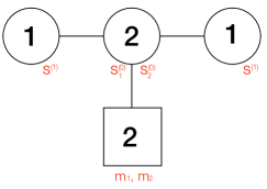
Coincidentally, the proper mirror pair consists of the two theories which we have already described in the previous section: A-models with labels (1,0)(2,2)(1,0)102210(1,0)(2,2)(1,0) (see Fig. 2, 3) and B-model, which is U(2)𝑈2U(2) theory with 4 flavors.

Refer to caption
Figure 3: A3subscript𝐴3A_{3} quiver with labels (1,0)1(2,2)0(1,2)2subscript101subscript220subscript122(1,0)_{1}(2,2)_{0}(1,2)_{2} together with all Coulomb branch parameters and masses.

We have concluded that these two theories are mirror dual to each other by applying the S-duality to their brane descriptions. Now we shall look at these two models more carefully by studying their supersymmetric vacua.

The vacua of the A quiver are governed by the following Bethe-type equations444We shall be using two terms – “Bethe equations” and “SUSY vacua equations” in the paper interchangeably.

τ2τ1a=12ησ(1)σa(0)ησa(0)σ(1)subscript𝜏2subscript𝜏1superscriptsubscriptproduct𝑎12𝜂superscript𝜎1subscriptsuperscript𝜎0𝑎𝜂subscriptsuperscript𝜎0𝑎superscript𝜎1\displaystyle\frac{\tau_{2}}{\tau_{1}}\prod_{a=1}^{2}\frac{\eta\sigma^{(1)}-\sigma^{(0)}_{a}}{\eta\sigma^{(0)}_{a}-\sigma^{(1)}} =1,absent1\displaystyle=1\,,
τ4τ3a=12ησ(2)σa(0)ησa(0)σ(2)subscript𝜏4subscript𝜏3superscriptsubscriptproduct𝑎12𝜂superscript𝜎2subscriptsuperscript𝜎0𝑎𝜂subscriptsuperscript𝜎0𝑎superscript𝜎2\displaystyle\frac{\tau_{4}}{\tau_{3}}\prod_{a=1}^{2}\frac{\eta\sigma^{(2)}-\sigma^{(0)}_{a}}{\eta\sigma^{(0)}_{a}-\sigma^{(2)}} =1,absent1\displaystyle=1\,,
τ3τ2I=12ησ1(0)σ(I)ησ(I)σ1(0)a=12ησ1(0)μa(0)ημa(0)σ1(0)η1σ1(0)ησ2(0)η1σ2(0)ησ1(0)subscript𝜏3subscript𝜏2superscriptsubscriptproduct𝐼12𝜂subscriptsuperscript𝜎01superscript𝜎𝐼𝜂superscript𝜎𝐼subscriptsuperscript𝜎01superscriptsubscriptproduct𝑎12𝜂subscriptsuperscript𝜎01subscriptsuperscript𝜇0𝑎𝜂subscriptsuperscript𝜇0𝑎subscriptsuperscript𝜎01superscript𝜂1subscriptsuperscript𝜎01𝜂subscriptsuperscript𝜎02superscript𝜂1subscriptsuperscript𝜎02𝜂subscriptsuperscript𝜎01\displaystyle\frac{\tau_{3}}{\tau_{2}}\prod_{I=1}^{2}\frac{\eta\sigma^{(0)}_{1}-\sigma^{(I)}}{\eta\sigma^{(I)}-\sigma^{(0)}_{1}}\cdot\prod_{a=1}^{2}\frac{\eta\sigma^{(0)}_{1}-\mu^{(0)}_{a}}{\eta\mu^{(0)}_{a}-\sigma^{(0)}_{1}}\cdot\frac{\eta^{-1}\sigma^{(0)}_{1}-\eta\sigma^{(0)}_{2}}{\eta^{-1}\sigma^{(0)}_{2}-\eta\sigma^{(0)}_{1}} =1,absent1\displaystyle=1\,, (19)
τ3τ2I=12ησ2(0)σ(I)ησ(I)σ2(0)a=12ησ2(0)μa(0)ημa(0)σ2(0)η1σ2(0)ησ1(0)η1σ1(0)ησ2(0)subscript𝜏3subscript𝜏2superscriptsubscriptproduct𝐼12𝜂subscriptsuperscript𝜎02superscript𝜎𝐼𝜂superscript𝜎𝐼subscriptsuperscript𝜎02superscriptsubscriptproduct𝑎12𝜂subscriptsuperscript𝜎02subscriptsuperscript𝜇0𝑎𝜂subscriptsuperscript𝜇0𝑎subscriptsuperscript𝜎02superscript𝜂1subscriptsuperscript𝜎02𝜂subscriptsuperscript𝜎01superscript𝜂1subscriptsuperscript𝜎01𝜂subscriptsuperscript𝜎02\displaystyle\frac{\tau_{3}}{\tau_{2}}\prod_{I=1}^{2}\frac{\eta\sigma^{(0)}_{2}-\sigma^{(I)}}{\eta\sigma^{(I)}-\sigma^{(0)}_{2}}\cdot\prod_{a=1}^{2}\frac{\eta\sigma^{(0)}_{2}-\mu^{(0)}_{a}}{\eta\mu^{(0)}_{a}-\sigma^{(0)}_{2}}\cdot\frac{\eta^{-1}\sigma^{(0)}_{2}-\eta\sigma^{(0)}_{1}}{\eta^{-1}\sigma^{(0)}_{1}-\eta\sigma^{(0)}_{2}} =1.absent1\displaystyle=1\,.

These four equations are to be solved with respect to four A-model Coulomb branch parameters: σ(1),σ1(0),σ2(0)superscript𝜎1subscriptsuperscript𝜎01subscriptsuperscript𝜎02\sigma^{(1)},\sigma^{(0)}_{1},\sigma^{(0)}_{2} and σ(2)superscript𝜎2\sigma^{(2)}, where upper indices designate the corresponding gauge groups in the quiver (see Fig. 3). Recall that FI terms t1subscript𝑡1t_{1} through t4subscript𝑡4t_{4} denote the coordinates of the NS5 branes along the x3superscript𝑥3x^{3} direction (see Fig. 2) and their differences t2t1,t3t2,t4t3subscript𝑡2subscript𝑡1subscript𝑡3subscript𝑡2subscript𝑡4subscript𝑡3t_{2}-t_{1},t_{3}-t_{2},t_{4}-t_{3} give the FI couplings. Note also that (3.1) contains all these variables in a trigonometric form, see (5) and (7). The first and the second equations of (3.1) arise from minimizing the effective twisted superpotential of the theory with respect to s(1)superscript𝑠1s^{(1)} and s(2)superscript𝑠2s^{(2)} respectively. These two Coulomb coordinates only appear in the bifundamental hypermultiplets (chiral parts inside those hypers contribute to the numerators, anti-chiral parts give the denominators) which connect nodes (1) and (0) and nodes (2) and (0); that is why the corresponding Bethe equations are fairly simple. At the middle node (0), however, there are more contributions. First, there are two variables s1(0)subscriptsuperscript𝑠01s^{(0)}_{1} and s2(0)subscriptsuperscript𝑠02s^{(0)}_{2} for each Cartan generator of U(2)𝑈2U(2), so there is a contribution from the adjoint field, and second, in addition to the bifundamental fields there are two more fundamental hypers with masses m1(0)subscriptsuperscript𝑚01m^{(0)}_{1} and m2(0)subscriptsuperscript𝑚02m^{(0)}_{2}. Note that 𝒩=2𝒩superscript2{\cal N}=2^{*} mass ϵitalic-ϵ\epsilon enters differently in the expressions for chiral and vector fields due to the special R-charge assignments: chiral fields have charge 111 and vectors fields have charge 22-2. We refer the reader to Gaiotto:2013bwa for more details.

In order to fully describe the parameter space {\cal L} in addition to writing Bethe equations (8), which can be viewed as

pσi(I)=1,i=1,NI,I=1,,L,formulae-sequencesuperscriptsubscript𝑝𝜎𝑖𝐼1formulae-sequence𝑖1subscript𝑁𝐼𝐼1𝐿p_{\sigma\,i}^{(I)}=1\,,\quad i=1,\dots N_{I}\,,\quad I=1,\dots,L\,, (20)

we specify the momenta conjugate to the mass parameters and FI parameters. For the case in hand we have for the middle node555For this example we omit the (0)0(0) superscript for the masses.

pμa=τ1τ2j=12ημaσj(0)ησj(0)μa,superscriptsubscript𝑝𝜇𝑎subscript𝜏1subscript𝜏2superscriptsubscriptproduct𝑗12𝜂subscript𝜇𝑎subscriptsuperscript𝜎0𝑗𝜂subscriptsuperscript𝜎0𝑗subscript𝜇𝑎p_{\mu}^{a}=\tau_{1}\tau_{2}\prod_{j=1}^{2}\frac{\eta\mu_{a}-\sigma^{(0)}_{j}}{\eta\sigma^{(0)}_{j}-\mu_{a}}\,, (21)

together with the corresponding formulae for pτsubscript𝑝𝜏p_{\tau}.

Already at this point we can make an interesting observation. Let us treat one of the equations (say for m1subscript𝑚1m_{1}) in (21) as a new Bethe equation (we shall now formally relabel m1subscript𝑚1m_{1} into σ(3)superscript𝜎3\sigma^{(3)}) as if the momentum pμ1superscriptsubscript𝑝𝜇1p_{\mu}^{1} is fixed to some constant value. One can now rewrite this equation as follows

τ1τ2pμ3j=12ησ(3)σj(0)ησj(0)σ(3)=1.subscript𝜏1subscript𝜏2superscriptsubscript𝑝𝜇3superscriptsubscriptproduct𝑗12𝜂superscript𝜎3subscriptsuperscript𝜎0𝑗𝜂subscriptsuperscript𝜎0𝑗superscript𝜎31\frac{\tau_{1}\tau_{2}}{p_{\mu}^{3}}\prod_{j=1}^{2}\frac{\eta\sigma^{(3)}-\sigma^{(0)}_{j}}{\eta\sigma^{(0)}_{j}-\sigma^{(3)}}=1\,. (22)

We now add this equation to (3.1) in order to form a new set of Bethe equations with respect to five variables: four Coulomb coordinates of the A3subscript𝐴3A_{3} quiver we have started with and σ(3)superscript𝜎3\sigma^{(3)}. One recognizes in this set of five equations the vacua equations for D4subscript𝐷4D_{4} quiver with U(2)𝑈2U(2) gauge group in the middle (label (0)0(0)) node, three U(1)𝑈1U(1) gauge nodes labeled by (1)(3)13(1)-(3), and one global U(1)𝑈1U(1) symmetry Fig. 4.

Refer to caption
Refer to caption
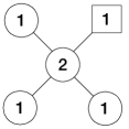
Figure 4: D4subscript𝐷4D_{4} quiver and its mirror dual obtained from the mirror pair of linear quivers with labels (1,0)(2,2)(1,2)102212(1,0)(2,2)(1,2) and (2,4)24(2,4).

From the point of view of the parameter space of the mirror theory fixing the momentum in (22), which is equivalent to losing mass parameter m1subscript𝑚1m_{1} (because we now need to solve the new set of equations with respect to it) corresponds to (up to some rescaling, which we shall fix promptly) eliminating one of the FI parameters. Indeed, according to the mirror map in the linear quivers FI parameters and masses get interchanged, as well as their conjugate momenta; so removing m1subscript𝑚1m_{1} on the A-side corresponds to eliminating, say, τ1subscriptsuperscript𝜏1\tau^{\vee}_{1} on the B-side. An exact expression for m1subscript𝑚1m_{1} as a solution of the A model Bethe equations may be quite cumbersome, and requires the knowledge of the solution of some high-degree polynomial equations. However, in order to identify the content of the B model after fixing pμ1superscriptsubscript𝑝𝜇1p_{\mu}^{1} we can use the expression for the momentum conjugate to τ1subscriptsuperscript𝜏1\tau^{\vee}_{1}. Recall that in our case the mirror quiver is A1subscript𝐴1A_{1} with labels (2,4)24(2,4), so it has two FI parameters: τ1subscriptsuperscript𝜏1\tau^{\vee}_{1} and τ2subscriptsuperscript𝜏2\tau^{\vee}_{2} and two Coulomb parameters σ1subscriptsuperscript𝜎1\sigma^{\vee}_{1} and σ2subscriptsuperscript𝜎2\sigma^{\vee}_{2}. According to Gaiotto:2013bwa we have

pτ 1=1σ1σ2.subscriptsuperscript𝑝1𝜏1subscriptsuperscript𝜎1subscriptsuperscript𝜎2p^{\vee\,1}_{\tau}=\frac{1}{\sigma^{\vee}_{1}\sigma^{\vee}_{2}}\,. (23)

We recall that under the mirror map μa=τasubscriptsuperscript𝜇𝑎subscript𝜏𝑎\mu^{\vee}_{a}=\tau_{a}. Our prescription now requires to us to fix pτ 1=1subscriptsuperscript𝑝1𝜏1p^{\vee\,1}_{\tau}=1, therefore we impose a constraint for σ1subscriptsuperscript𝜎1\sigma^{\vee}_{1} and σ2subscriptsuperscript𝜎2\sigma^{\vee}_{2}, namely that one variable is inversely proportional to another, or, in terms of rational coordinates, s1=s2subscriptsuperscript𝑠1subscriptsuperscript𝑠2s^{\vee}_{1}=-s^{\vee}_{2}. This constraint yields us SU(2)=Sp(1)𝑆𝑈2𝑆𝑝1SU(2)=Sp(1) gauge theory with four flavors. Therefore we have shown how the parameter spaces of the two mirror quivers in Fig. 4 can be embedded inside the parameter spaces of two linear quivers.

The statement will become obvious upon proper identification of the momentum (21) with the twist parameters of the A quiver. It works as follows

τ1τ2pμ1=τ2τ1,subscript𝜏1subscript𝜏2superscriptsubscript𝑝𝜇1subscript𝜏2subscript𝜏1\frac{\tau_{1}\tau_{2}}{p_{\mu}^{1}}=\frac{\tau_{2}}{\tau_{1}}\,, (24)

therefore pμ1=τ12superscriptsubscript𝑝𝜇1superscriptsubscript𝜏12p_{\mu}^{1}=\tau_{1}^{2}. In order to match it with pτ 1=1subscriptsuperscript𝑝1𝜏1p^{\vee\,1}_{\tau}=1, which we just used to derive the Sp(1)𝑆𝑝1Sp(1) theory we need to assume τ12=1subscriptsuperscript𝜏211\tau^{2}_{1}=1 or t1=0subscript𝑡10t_{1}=0, which in terms of the brane construction of Fig. 2 fixes the location of the location of the leftmost NS fivebrane to the origin in the x3superscript𝑥3x^{3} direction.

In a moment we shall demonstrate how the procedure we have just performed (also known as gauging of an Abelian symmetry, or merely Abelian gauging) can also be carried out at the level of partition functions of the A and B models (13), (14). This computation will turn out to be very effective in deriving mirror pairs via Abelian gauging as well as obtaining exact relationships between the mass parameters/FI parameters of the dual theories (so called mirror maps).

The dimensions of the Coulomb and Higgs branches of the A-model quiver before the gauging Fig. 3 were 444 and 222 respectively (correspondingly these numbers give the dimensions of the Higgs and Coulomb branches of the B-model before the gauging). After gauging these dimensions on the A-side (see Fig. 4) have become 555 and 111 respectively, which agrees with the dimensions of the Higgs and Coulomb branches of the Sp(1)𝑆𝑝1Sp(1) theory with four flavors. Therefore we can see that by gauging a U(1)𝑈1U(1) subgroup of the U(2)𝑈2U(2) node on the left in Fig. 6 we increase the dimension of the Coulomb branch by one and decrease the dimension of the Higgs branch by one.

As we have already mentioned before, the mirror map (exact correspondence of the mass/FI parameters on both sides of the duality) for linear quivers is very simple. Indeed, one simply interchanges the roles of twisted masses and FI parameters. However, after the gauging has been implemented, the mirror map will change as well. In order to derive the exact form of this map, as well as verify the proposed mirror pair using exact localization methods, we appeal to the computations of partition function on a three-sphere.

3.2 Partition Function Approach

For gauging the U(2)𝑈2U(2) flavor symmetry we have to treat m1subscript𝑚1m_{1} and m2subscript𝑚2m_{2} as independent parameters, without imposing any constraints. Note that from (13) and (14) we have

𝒵A=e2πim1(t1+t2)e2πim2(t3+t4)𝒵B.subscript𝒵𝐴superscript𝑒2𝜋𝑖subscript𝑚1subscript𝑡1subscript𝑡2superscript𝑒2𝜋𝑖subscript𝑚2subscript𝑡3subscript𝑡4subscript𝒵𝐵{\cal Z}_{A}=e^{-2\pi im_{1}(t_{1}+t_{2})}e^{2\pi im_{2}(t_{3}+t_{4})}{\cal Z}_{B}\,. (25)

Now let us implement the gauging by m1(t~1)s3subscript𝑚1subscript~𝑡1subscript𝑠3m_{1}(\widetilde{t}_{1})\to-s_{3}. Since we are gauging a single U(1)𝑈1U(1) flavor symmetry, the partition function of gauged A-model (which we denote by 𝒵~Asubscript~𝒵𝐴\widetilde{{\cal Z}}_{A}) may be simply obtained by multiplying 𝒵Asubscript𝒵𝐴{\cal Z}_{A} with the appropriate FI contribution e2πiη3s3superscript𝑒2𝜋𝑖subscript𝜂3subscript𝑠3e^{-2\pi i{\eta}_{3}s_{3}} and integrating over s3subscript𝑠3s_{3}. Therefore,

𝒵~A(1)=𝑑s3e2πiη3s3𝒵A=α=12dsαds3d2s02!e2πiη3s3α=12e2πisαηαi=12e2πis0iη0sinh2π(s01s02)i=12coshπ(s1s0i)coshπ(s0is3)coshπ(s2s0i)coshπ(s0i+m2)=e2πim2(t3+t4)𝑑s3e2πis3(t1+t2)e2πiη3s3𝒵B=e2πim2(t3+t4)𝑑s3e2πis3(t1+t2)e2πiη3s3d2s2!i=12e2πisiηsinh2π(s1s2)i=12a=14coshπ(si+Ma).subscriptsuperscript~𝒵1𝐴differential-dsubscript𝑠3superscript𝑒2𝜋𝑖subscript𝜂3subscript𝑠3subscript𝒵𝐴subscriptsuperscriptproduct2𝛼1𝑑subscript𝑠𝛼𝑑subscript𝑠3superscript𝑑2subscript𝑠02superscript𝑒2𝜋𝑖subscript𝜂3subscript𝑠3subscriptsuperscriptproduct2𝛼1superscript𝑒2𝜋𝑖subscript𝑠𝛼subscript𝜂𝛼subscriptsuperscriptproduct2𝑖1superscript𝑒2𝜋𝑖subscriptsuperscript𝑠𝑖0subscript𝜂0superscript2𝜋subscriptsuperscript𝑠10subscriptsuperscript𝑠20subscriptsuperscriptproduct2𝑖1𝜋subscript𝑠1subscriptsuperscript𝑠𝑖0𝜋subscriptsuperscript𝑠𝑖0subscript𝑠3𝜋subscript𝑠2subscriptsuperscript𝑠𝑖0𝜋subscriptsuperscript𝑠𝑖0subscript𝑚2superscript𝑒2𝜋𝑖subscript𝑚2subscript𝑡3subscript𝑡4differential-dsubscript𝑠3superscript𝑒2𝜋𝑖subscript𝑠3subscript𝑡1subscript𝑡2superscript𝑒2𝜋𝑖subscript𝜂3subscript𝑠3subscript𝒵𝐵superscript𝑒2𝜋𝑖subscript𝑚2subscript𝑡3subscript𝑡4differential-dsubscript𝑠3superscript𝑒2𝜋𝑖subscript𝑠3subscript𝑡1subscript𝑡2superscript𝑒2𝜋𝑖subscript𝜂3subscript𝑠3superscript𝑑2𝑠2subscriptsuperscriptproduct2𝑖1superscript𝑒2𝜋𝑖superscript𝑠𝑖𝜂superscript2𝜋superscript𝑠1superscript𝑠2subscriptsuperscriptproduct2𝑖1subscriptsuperscriptproduct4𝑎1𝜋superscript𝑠𝑖subscript𝑀𝑎\begin{split}\widetilde{{\cal Z}}^{(1)}_{A}&=\int ds_{3}e^{-2\pi i{\eta}_{3}s_{3}}{\cal Z}_{A}\\ &=\int\prod^{2}_{\alpha=1}ds_{\alpha}ds_{3}\frac{d^{2}s_{0}}{2!}\frac{e^{-2\pi i{\eta}_{3}s_{3}}\prod^{2}_{\alpha=1}e^{2\pi is_{\alpha}\eta_{\alpha}}\prod^{2}_{i=1}e^{2\pi is^{i}_{0}\eta_{0}}\sinh^{2}{\pi(s^{1}_{0}-s^{2}_{0})}}{\prod^{2}_{i=1}\cosh{\pi(s_{1}-s^{i}_{0})}\cosh{\pi(s^{i}_{0}-s_{3})}\cosh{\pi(s_{2}-s^{i}_{0})}\cosh{\pi(s^{i}_{0}+m_{2})}}\\ &=e^{2\pi im_{2}(t_{3}+t_{4})}\int ds_{3}e^{-2\pi is_{3}(t_{1}+t_{2})}e^{-2\pi i{\eta}_{3}s_{3}}{\cal Z}_{B}\\ &=e^{2\pi im_{2}(t_{3}+t_{4})}\int ds_{3}e^{-2\pi is_{3}(t_{1}+t_{2})}e^{-2\pi i{\eta}_{3}s_{3}}\frac{d^{2}s}{2!}\frac{\prod^{2}_{i=1}e^{2\pi is^{i}\eta}\sinh^{2}{\pi(s^{1}-s^{2})}}{\prod^{2}_{i=1}\prod^{4}_{a=1}\cosh{\pi(s^{i}+M_{a})}}\,.\end{split} (26)

The partition function 𝒵~A(1)subscriptsuperscript~𝒵1𝐴\widetilde{{\cal Z}}^{(1)}_{A} corresponds to the gauged A-model quiver which, from the second line, is a U(1)3×U(2)𝑈superscript13𝑈2U(1)^{3}\times U(2) gauge theory with one fundamental hyper (Fig. 4). To determine the mirror of this quiver, one needs to consider the formula on the third line, which essentially rewrites the partition function of the gauged A-model quiver in terms of the partition function of the original B-model. One may then identify the dual theory by computing 𝒵~A(1)subscriptsuperscript~𝒵1𝐴\widetilde{{\cal Z}}^{(1)}_{A} using the third/fourth line of the above equation.

𝒵~A(1)=e2πim2(t3+t4)𝑑s3d2s2!sinh2π(s1s2)i=12a=14coshπ(si+Ma)i=12e2πisi(m2+s3)e2πis3(t1t2η3)=e2πim2(t3+t4)d2s2!sinh2π(s1s2)δ(s1+s2t1t2η3)i=12a=14coshπ(si+Ma)e2πim2(s1+s2)=e2πim2(t1t2η3+t3+t4)d2s2!sinh2π(s1s2)δ(s1+s2)i=12a=14coshπ(si+(t1+t2+η3)/2+Ma).subscriptsuperscript~𝒵1𝐴superscript𝑒2𝜋𝑖subscript𝑚2subscript𝑡3subscript𝑡4differential-dsubscript𝑠3superscript𝑑2𝑠2superscript2𝜋superscript𝑠1superscript𝑠2subscriptsuperscriptproduct2𝑖1subscriptsuperscriptproduct4𝑎1𝜋superscript𝑠𝑖subscript𝑀𝑎subscriptsuperscriptproduct2𝑖1superscript𝑒2𝜋𝑖superscript𝑠𝑖subscript𝑚2subscript𝑠3superscript𝑒2𝜋𝑖subscript𝑠3subscript𝑡1subscript𝑡2subscript𝜂3superscript𝑒2𝜋𝑖subscript𝑚2subscript𝑡3subscript𝑡4superscript𝑑2𝑠2superscript2𝜋superscript𝑠1superscript𝑠2𝛿superscript𝑠1superscript𝑠2subscript𝑡1subscript𝑡2subscript𝜂3subscriptsuperscriptproduct2𝑖1subscriptsuperscriptproduct4𝑎1𝜋superscript𝑠𝑖subscript𝑀𝑎superscript𝑒2𝜋𝑖subscript𝑚2superscript𝑠1superscript𝑠2superscript𝑒2𝜋𝑖subscript𝑚2subscript𝑡1subscript𝑡2subscript𝜂3subscript𝑡3subscript𝑡4superscript𝑑2𝑠2superscript2𝜋superscript𝑠1superscript𝑠2𝛿superscript𝑠1superscript𝑠2subscriptsuperscriptproduct2𝑖1subscriptsuperscriptproduct4𝑎1𝜋superscript𝑠𝑖subscript𝑡1subscript𝑡2subscript𝜂32subscript𝑀𝑎\begin{split}&\widetilde{{\cal Z}}^{(1)}_{A}=e^{2\pi im_{2}(t_{3}+t_{4})}\int ds_{3}\frac{d^{2}s}{2!}\frac{\sinh^{2}{\pi(s^{1}-s^{2})}}{\prod^{2}_{i=1}\prod^{4}_{a=1}\cosh{\pi(s^{i}+M_{a})}}\prod^{2}_{i=1}e^{2\pi is^{i}(-m_{2}+s_{3})}e^{2\pi is_{3}(-t_{1}-t_{2}-{\eta}_{3})}\\ &=e^{2\pi im_{2}(t_{3}+t_{4})}\int\frac{d^{2}s}{2!}\frac{\sinh^{2}{\pi(s^{1}-s^{2})}\delta\left(s^{1}+s^{2}-t_{1}-t_{2}-{\eta}_{3}\right)}{\prod^{2}_{i=1}\prod^{4}_{a=1}\cosh{\pi(s^{i}+M_{a})}}e^{-2\pi im_{2}(s^{1}+s^{2})}\\ &=e^{2\pi im_{2}(-t_{1}-t_{2}-{\eta}_{3}+t_{3}+t_{4})}\int\frac{d^{2}s}{2!}\frac{\sinh^{2}{\pi(s^{1}-s^{2})}\delta\left(s^{1}+s^{2}\right)}{\prod^{2}_{i=1}\prod^{4}_{a=1}\cosh{\pi(s^{i}+(t_{1}+t_{2}+{\eta}_{3})/2+M_{a})}}\,.\end{split} (27)

Therefore, up to the prefactor (a pure phase) indicated above, one can easily identify the above as the S3superscript𝑆3S^{3} partition function of a SU(2)𝑆𝑈2SU(2) gauge theory with 4 hypers. Note that the masses of the fundamental hypers are shifted as MaMa+(t1+t2+η3)/2subscript𝑀𝑎subscript𝑀𝑎subscript𝑡1subscript𝑡2subscript𝜂32M_{a}\to M_{a}+(t_{1}+t_{2}+{\eta}_{3})/2 as we gauge the flavor in the A-model. The mirror map for the mirror dual pair in Fig. 4 is therefore

Ma(1)=Ma+(t1+t2+η3)/2=ta+(t1+t2+η3)/2subscriptsuperscript𝑀1𝑎subscript𝑀𝑎subscript𝑡1subscript𝑡2subscript𝜂32subscript𝑡𝑎subscript𝑡1subscript𝑡2subscript𝜂32M^{(1)}_{a}=M_{a}+(t_{1}+t_{2}+{\eta}_{3})/2=t_{a}+(t_{1}+t_{2}+{\eta}_{3})/2 (28)

The mirror map is very similar to that of the original linear quiver pairs - each mass just gets shifted by the same factor. For the new mirror pair, the A-model has four independent FI parameters, namely tasubscript𝑡𝑎t_{a}s (a=1,2,3,4𝑎1234a=1,2,3,4) with one constraint and η3subscript𝜂3\eta_{3} -which matches the four independent masses in the B-model. Note that the masses of the B-model no longer satisfy the constraint of zero sum - in fact aMa(1)=2(t1+t2+η3)0subscript𝑎subscriptsuperscript𝑀1𝑎2subscript𝑡1subscript𝑡2subscript𝜂30\sum_{a}M^{(1)}_{a}=2(t_{1}+t_{2}+{\eta}_{3})\neq 0.

One can gauge the remaining U(1)𝑈1U(1) flavor in exactly the same way. In this case, one obtains,

𝒵~A(2)=δ(t1+t2+η3+η4t3t4)d2s2!sinh2π(s1s2)δ(s1+s2)i=12a=14coshπ(si+(t1+t2+η3)/2+ta)=δ(η1+η2+η3+η4+2η0)d2s2!sinh2π(s1s2)δ(s1+s2)i=12a=14coshπ(si+(t1+t2+η3)/2+ta).subscriptsuperscript~𝒵2𝐴𝛿subscript𝑡1subscript𝑡2subscript𝜂3subscript𝜂4subscript𝑡3subscript𝑡4superscript𝑑2𝑠2superscript2𝜋superscript𝑠1superscript𝑠2𝛿superscript𝑠1superscript𝑠2subscriptsuperscriptproduct2𝑖1subscriptsuperscriptproduct4𝑎1𝜋superscript𝑠𝑖subscript𝑡1subscript𝑡2subscript𝜂32subscript𝑡𝑎𝛿subscript𝜂1subscript𝜂2subscript𝜂3subscript𝜂42subscript𝜂0superscript𝑑2𝑠2superscript2𝜋superscript𝑠1superscript𝑠2𝛿superscript𝑠1superscript𝑠2subscriptsuperscriptproduct2𝑖1subscriptsuperscriptproduct4𝑎1𝜋superscript𝑠𝑖subscript𝑡1subscript𝑡2subscript𝜂32subscript𝑡𝑎\begin{split}\widetilde{{\cal Z}}^{(2)}_{A}=&\delta\left(t_{1}+t_{2}+{\eta}_{3}+{\eta}_{4}-t_{3}-t_{4}\right)\int\frac{d^{2}s}{2!}\frac{\sinh^{2}{\pi(s^{1}-s^{2})}\delta\left(s^{1}+s^{2}\right)}{\prod^{2}_{i=1}\prod^{4}_{a=1}\cosh{\pi(s^{i}+(t_{1}+t_{2}+{\eta}_{3})/2+t_{a})}}\\ =&\delta\left(\eta_{1}+\eta_{2}+{\eta}_{3}+{\eta}_{4}+2\eta_{0}\right)\int\frac{d^{2}s}{2!}\frac{\sinh^{2}{\pi(s^{1}-s^{2})}\delta\left(s^{1}+s^{2}\right)}{\prod^{2}_{i=1}\prod^{4}_{a=1}\cosh{\pi(s^{i}+(t_{1}+t_{2}+{\eta}_{3})/2+t_{a})}}\,.\end{split} (29)

The B-model is therefore the same, but the A-model will be D^4subscript^𝐷4\hat{D}_{4} quiver with an overall U(1)𝑈1U(1) removed as imposed by the delta function constraint in the previous equation.

η1+η2+2η0+η3+η4=0.subscript𝜂1subscript𝜂22subscript𝜂0subscript𝜂3subscript𝜂40\eta_{1}+\eta_{2}+2\eta_{0}+{\eta}_{3}+{\eta}_{4}=0\,. (30)

Note that the form of the constraint is of the form iηili=0subscript𝑖subscript𝜂𝑖subscript𝑙𝑖0\sum_{i}\eta_{i}l_{i}=0, where the sum runs over the nodes of the D^4subscript^𝐷4\hat{D}_{4} quiver while lisubscript𝑙𝑖l_{i} denotes the Dynkin label of the i𝑖i-th node.
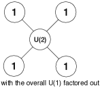
One therefore has a quiver with the gauge group U(1)4×U(2)//U(1)U(1)^{4}\times U(2)//U(1). On the B-model side, this simply amounts to imposing the constraint (30). The mirror map formally remains the same, subject to this extra constraint, see Fig. 5.
Refer to caption
Figure 5: D^4subscript^𝐷4\hat{D}_{4} with U(2)𝑈2U(2) gauge group in the middle node and overall U(1)𝑈1U(1) factored out. It may be considered as a result of two Abelian gaugings which were implemented on the middle node of the linear (2,0)(2,2)(2,0)202220(2,0)(2,2)(2,0) quiver.

One may wonder however if there is a preferred choice in imposing extra constraint (30). For instance, one could try to consider D^4subscript^𝐷4\hat{D}_{4} quiver with SU(2)𝑆𝑈2SU(2) node in the middle instead of the U(2)𝑈2U(2). As it turns out, this choice, as well as all the other U(1)𝑈1U(1) quotients, except for S(U(1)4×U(2))𝑆𝑈superscript14𝑈2S(U(1)^{4}\times U(2)) or the configuration presented in Fig. 4 where an overall U(1)𝑈1U(1) factor is decoupled, does not give a correct mirror description. Below we demonstrate this fact by computing the Hilbert series on the Coulomb branches Cremonesi:2013lqa of the corresponding D^4subscript^𝐷4\hat{D}_{4} quivers.

3.3 Checking mirror symmetry: The Hilbert series of D^4subscript^𝐷4\hat{D}_{4} quiver

The Hilbert series of D^4subscript^𝐷4\hat{D}_{4} quiver in Fig. 5 can be obtained via formula (16); the result is as follows:

H[D^4](t,𝒙)𝐻delimited-[]subscript^𝐷4𝑡𝒙\displaystyle H[\widehat{D}_{4}](t,\bm{x}) =m1,,m4n1n2=0tΔ(𝒎,𝒏)(z0n1+n2i=14zimi)×\displaystyle=\sum_{m_{1},\ldots,m_{4}\in\mathbb{Z}}\;\sum_{n_{1}\geq n_{2}=0}t^{\Delta(\bm{m},\bm{n})}\left(z_{0}^{n_{1}+n_{2}}\prod_{i=1}^{4}{z_{i}^{m_{i}}}\right)\times
[PU(1)(t)]4(1t)PU(2)(t,𝒏).superscriptdelimited-[]subscript𝑃𝑈1𝑡41𝑡subscript𝑃𝑈2𝑡𝒏\displaystyle\qquad\left[P_{U(1)}(t)\right]^{4}(1-t)P_{U(2)}(t,\bm{n})\,. (31)

Let us explain each part of the above formula as follows. The dimension formula of monopole operators is given by

Δ(𝒎,𝒏)=|n1n2|+12i=14j=12|minj|,Δ𝒎𝒏subscript𝑛1subscript𝑛212superscriptsubscript𝑖14superscriptsubscript𝑗12subscript𝑚𝑖subscript𝑛𝑗\displaystyle\Delta(\bm{m},\bm{n})=-|n_{1}-n_{2}|+\frac{1}{2}\sum_{i=1}^{4}\sum_{j=1}^{2}|m_{i}-n_{j}|~{}, (32)

where m1,,m4subscript𝑚1subscript𝑚4m_{1},\dots,m_{4} are monopole charges associated with each U(1)𝑈1U(1) group, and n1,n2subscript𝑛1subscript𝑛2n_{1},n_{2} are monopole charges associated with U(2)𝑈2U(2) in the center of the quiver. The product in the brackets in the first line of (3.3) corresponds to the refinement of various global charges: each fugacity zisubscript𝑧𝑖z_{i} keeps track of the charge misubscript𝑚𝑖m_{i} for each U(1)𝑈1U(1) and the fugacity z0subscript𝑧0z_{0} keeps track of the topological charge n1+n2subscript𝑛1subscript𝑛2n_{1}+n_{2} of U(2)𝑈2U(2). Functions PU(1)(t)subscript𝑃𝑈1𝑡P_{U(1)}(t) and PU(2)(t,𝒏)subscript𝑃𝑈2𝑡𝒏P_{U(2)}(t,\bm{n}) are contributions from the Casimir invariants of U(1)𝑈1U(1) and U(2)𝑈2U(2) gauge groups given by (17):

PU(1)(t)=11t,PU(2)(t,𝒏)={1(1t)(1t2),n1=n21(1t)2,n1n2.formulae-sequencesubscript𝑃𝑈1𝑡11𝑡subscript𝑃𝑈2𝑡𝒏cases11𝑡1superscript𝑡2subscript𝑛1subscript𝑛21superscript1𝑡2subscript𝑛1subscript𝑛2\displaystyle P_{U(1)}(t)=\frac{1}{1-t}~{},\qquad P_{U(2)}(t,\bm{n})=\begin{cases}\frac{1}{(1-t)(1-t^{2})}~{},&\qquad n_{1}=n_{2}\\ \frac{1}{(1-t)^{2}}~{},&\qquad n_{1}\neq n_{2}~{}.\end{cases} (33)

An overall U(1)𝑈1U(1) in the quiver Fig. 5 is factored out from the U(2)𝑈2U(2) middle node via the following steps:

  1. 1.

    fixing the charge n2subscript𝑛2n_{2} associated with U(2)𝑈2U(2) gauge group to zero, as stated in the second summation;

  2. 2.

    multiplying the factor (1t)1𝑡(1-t) in front of PU(2)(t,𝒏)subscript𝑃𝑈2𝑡𝒏P_{U(2)}(t,\bm{n}), and

  3. 3.

    by imposing the condition

    z02z1z2z3z4=1.superscriptsubscript𝑧02subscript𝑧1subscript𝑧2subscript𝑧3subscript𝑧41\displaystyle z_{0}^{2}z_{1}z_{2}z_{3}z_{4}=1~{}. (34)

Note that this procedure of gauge fixing is not unique. One can instead, for example, take any of the U(1)𝑈1U(1) nodes in Fig. 5 to be a flavour node (see e.g., section 3.4 of Cremonesi:2013lqa ) and obtain the same answer.

In order to make the SU(2)𝑆𝑈2SU(2) associated to each leg manifest and to fix the overall U(1)𝑈1U(1), we write

z0=x1x2x3x4,zi=xi2,formulae-sequencesubscript𝑧0subscript𝑥1subscript𝑥2subscript𝑥3subscript𝑥4subscript𝑧𝑖superscriptsubscript𝑥𝑖2\displaystyle z_{0}=x_{1}x_{2}x_{3}x_{4},\qquad z_{i}=x_{i}^{-2}~{}, (35)

where xisubscript𝑥𝑖x_{i} (with i=1,2,3,4𝑖1234i=1,2,3,4) are the SU(2)𝑆𝑈2SU(2) fugacities corresponding to each leg.

Since SU(2)𝑆𝑈2SU(2) gauge theory with 444 flavors has an SO(8)𝑆𝑂8SO(8) flavour symmetry, it is expected that the Hilbert series should be written in terms of characters of SO(8)𝑆𝑂8SO(8) representations. In order to do so, we may use the following fugacity map666This is the same as (4.5) of Hanany:2010qu

y1=x1x2,y2=x22,y3=x3x2,y4=x4x2,formulae-sequencesubscript𝑦1subscript𝑥1subscript𝑥2formulae-sequencesubscript𝑦2superscriptsubscript𝑥22formulae-sequencesubscript𝑦3subscript𝑥3subscript𝑥2subscript𝑦4subscript𝑥4subscript𝑥2\displaystyle y_{1}=x_{1}x_{2},\quad y_{2}=x_{2}^{2},\quad y_{3}=x_{3}x_{2},\quad y_{4}=x_{4}x_{2}~{}, (36)

where y1,y2,y3,y4subscript𝑦1subscript𝑦2subscript𝑦3subscript𝑦4y_{1},y_{2},y_{3},y_{4} are the SO(8)𝑆𝑂8SO(8) fugacities and x1,x2,x3,x4subscript𝑥1subscript𝑥2subscript𝑥3subscript𝑥4x_{1},x_{2},x_{3},x_{4} are the SU(2)4𝑆𝑈superscript24SU(2)^{4} fugacities. To make a connection with the fugacities z0,z1,,z4subscript𝑧0subscript𝑧1subscript𝑧4z_{0},z_{1},\ldots,z_{4}, we have

z0=y1y21y3y4,z1=y12y21,z2=y2,z3=y21y32,z4=y21y42.formulae-sequencesubscript𝑧0subscript𝑦1superscriptsubscript𝑦21subscript𝑦3subscript𝑦4formulae-sequencesubscript𝑧1superscriptsubscript𝑦12superscriptsubscript𝑦21formulae-sequencesubscript𝑧2subscript𝑦2formulae-sequencesubscript𝑧3superscriptsubscript𝑦21superscriptsubscript𝑦32subscript𝑧4superscriptsubscript𝑦21superscriptsubscript𝑦42\displaystyle z_{0}=y_{1}y_{2}^{-1}y_{3}y_{4}~{},\quad z_{1}=y_{1}^{2}y_{2}^{-1},\quad z_{2}=y_{2},\quad z_{3}=y_{2}^{-1}y_{3}^{2},\quad z_{4}=y_{2}^{-1}y_{4}^{2}~{}. (37)

In terms of y1,,y4subscript𝑦1subscript𝑦4y_{1},\ldots,y_{4}, the power series of (3.3) in t𝑡t is given by

H[D^4](t,𝒚)=k=0[0,k,0,0]𝒚tk,𝐻delimited-[]subscript^𝐷4𝑡𝒚superscriptsubscript𝑘0subscript0𝑘00𝒚superscript𝑡𝑘\displaystyle H[\widehat{D}_{4}](t,\bm{y})=\sum_{k=0}^{\infty}[0,k,0,0]_{\bm{y}}t^{k}~{}, (38)

where [0,k,0,0]𝒚subscript0𝑘00𝒚[0,k,0,0]_{\bm{y}} denotes the character of representation [0,k,0,0]0𝑘00[0,k,0,0] of SO(8)𝑆𝑂8SO(8) written in terms of y1,,y4subscript𝑦1subscript𝑦4y_{1},\ldots,y_{4}. Henceforth, we use a square bracket []𝒚subscriptdelimited-[]𝒚[\ldots]_{\bm{y}} to denote the character of our representation written in terms of the variables in the subscript, which is 𝒚𝒚\bm{y} in this case.777The characters can be computed using Weyl’s character formula or using LiE online service in the following link: http://young.sp2mi.univ-poitiers.fr/cgi-bin/form-prep/marc/LiE_form.act?action=character&type=D&rank=4&highest_rank=8. To avoid the cumbersome notation, we drop the subscript when there is no potential confusion.

Setting yi=1subscript𝑦𝑖1y_{i}=1, which amounts to taking the dimension of the representations in (38), we obtain the unrefined Hilbert series

H[D^4](t,{yi=1})𝐻delimited-[]subscript^𝐷4𝑡subscript𝑦𝑖1\displaystyle H[\widehat{D}_{4}](t,\{y_{i}=1\}) =k=0dim[0,k,0,0]tkabsentsuperscriptsubscript𝑘0dimension0𝑘00superscript𝑡𝑘\displaystyle=\sum_{k=0}^{\infty}\dim~{}[0,k,0,0]t^{k}
=k=0(k+1)(k+2)3(k+3)3(k+4)(2k+5)4320tkabsentsuperscriptsubscript𝑘0𝑘1superscript𝑘23superscript𝑘33𝑘42𝑘54320superscript𝑡𝑘\displaystyle=\sum_{k=0}^{\infty}\frac{(k+1)(k+2)^{3}(k+3)^{3}(k+4)(2k+5)}{4320}t^{k}
=(1+t)(1+17t+48t2+17t3+t4)(1t)10absent1𝑡117𝑡48superscript𝑡217superscript𝑡3superscript𝑡4superscript1𝑡10\displaystyle=\frac{(1+t)(1+17t+48t^{2}+17t^{3}+t^{4})}{(1-t)^{10}}
=1+28t+300t2+1925t3+8918t4+.absent128𝑡300superscript𝑡21925superscript𝑡38918superscript𝑡4\displaystyle=1+28t+300t^{2}+1925t^{3}+8918t^{4}+\ldots~{}. (39)
A remark on gauge fixing.

We emphasize that the gauge fixing procedure described above is different from taking the middle node of Fig. 5 to be SU(2)𝑆𝑈2SU(2). Let us compare (3.3) with the Hilbert series of the same quiver with the central node taken to be SU(2)𝑆𝑈2SU(2). The latter is given by

H~(t,𝒙)~𝐻𝑡𝒙\displaystyle\widetilde{H}(t,\bm{x}) =m1,,m4n=0tΔ~(𝒎,𝒏)(i=14xi2mi)×\displaystyle=\sum_{m_{1},\ldots,m_{4}\in\mathbb{Z}}\;\sum_{n=0}^{\infty}t^{\widetilde{\Delta}(\bm{m},\bm{n})}\left(\prod_{i=1}^{4}{x_{i}^{-2m_{i}}}\right)\times
[PU(1)(t)]4(1t)PU(2)(t,n,n),superscriptdelimited-[]subscript𝑃𝑈1𝑡41𝑡subscript𝑃𝑈2𝑡𝑛𝑛\displaystyle\qquad\left[P_{U(1)}(t)\right]^{4}(1-t)P_{U(2)}(t,n,-n)~{}, (40)

where

Δ~(𝒎,n)=|2n|+12i=14j=12(|min|+|mi+n|).~Δ𝒎𝑛2𝑛12superscriptsubscript𝑖14superscriptsubscript𝑗12subscript𝑚𝑖𝑛subscript𝑚𝑖𝑛\displaystyle\widetilde{\Delta}(\bm{m},n)=-|2n|+\frac{1}{2}\sum_{i=1}^{4}\sum_{j=1}^{2}(|m_{i}-n|+|m_{i}+n|)~{}. (41)

Indeed, the summand of (3.3) is equal to that of (3.3) with n1=n2=nsubscript𝑛1subscript𝑛2𝑛n_{1}=n_{2}=-n. However, after taking the summations into account, we see that this is not compatible with the gauge fixing described above, where we fixed n2=0subscript𝑛20n_{2}=0 rather than taking n2subscript𝑛2n_{2} to be n1subscript𝑛1-n_{1}. For reference, we present a few terms of (3.3):

H~(t,{xi=1})~𝐻𝑡subscript𝑥𝑖1\displaystyle\widetilde{H}(t,\{x_{i}=1\}) =1+12t+156t2+949t3+4486t4+.absent112𝑡156superscript𝑡2949superscript𝑡34486superscript𝑡4\displaystyle=1+12t+156t^{2}+949t^{3}+4486t^{4}+\ldots~{}. (42)

This is different from (3.3).

In the following section, while discussing a balanced or any generic flavorless 3d quiver, we will implicitly assume that an overall U(1)𝑈1U(1) vector multiplet decouples from the theory. Note that in the classical analysis of the parameter space of vacua {\cal L} there is a notion of the “center of mass” for twisted masses and FI terms, which is naturally associated with the translational symmetry of the system of D5 and NS5 branes. Therefore one can gauge the entire global symmetry of the quiver on the level of {\cal L}, except for a single U(1)𝑈1U(1) factor. This is the reason why in the A model quiver in Fig. 4 one global U(1)𝑈1U(1) symmetry is present. However, as we have shown above, the Hilbert series for this quiver and for balanced flavorless D^4subscript^𝐷4\hat{D}_{4} from Fig. 5 are identical. Classically the statement boils down to the fact that a linear rank-L𝐿L quiver has L+1𝐿1L+1 NS5 branes and therefore L+1𝐿1L+1 NS5 positions. However, the FI parameters appearing in the 𝒩=4𝒩4\mathcal{N}=4 Lagrangian correspond to the differences ηi=ti+1tisubscript𝜂𝑖subscript𝑡𝑖1subscript𝑡𝑖\eta_{i}=t_{i+1}-t_{i}. In the remainder of the paper we shall be using this observation – by specifying a proper submanifold in {\cal L} and obtaining a quiver with a single global U(1)𝑈1U(1) symmetry we will automatically arrive at the corresponding flavorless quiver and its mirror description.

The rest of the paper consists of the analysis of 3d mirror pairs involving quivers of different shapes: generic D^Nsubscript^𝐷𝑁\hat{D}_{N} and star-shaped quivers in the next section, exceptional E6,7,8subscript𝐸678E_{6,7,8} quivers and their extensions in Sec. 5, and framed A1subscript𝐴1A_{1} Sp(Nc)𝑆𝑝subscript𝑁𝑐Sp(N_{c}) quivers in Sec. 6.

4 D^Nsubscript^𝐷𝑁\hat{D}_{N} and Star-shaped Quivers

In this section, we analyze various examples of the framed D^Nsubscript^𝐷𝑁\hat{D}_{N} quivers shown in Tab. 1 and closely related star-shaped quivers using the Abelian gauging technique.

A straightforward generalization of the D^4subscript^𝐷4\hat{D}_{4} quiver from Fig. 5 is a star-shaped quiver with more than four nodes with U(1)𝑈1U(1) gauge groups on those nodes. Later we shall also discuss star quivers with longer legs.

4.1 Star-shaped Quivers via Abelian Gauging

Let us consider an obvious generalization of the example from Fig. 4.

Consider a mirror pair of linear quivers (Fig. 6) where the A-model is (1,0)(2,N)(1,0)102𝑁10(1,0)(2,N)(1,0) quiver and the B-model is (2,2)1(2,0)2(2,0)N2(2,2)N1subscript221subscript202subscript20𝑁2subscript22𝑁1(2,2)_{1}(2,0)_{2}\cdots(2,0)_{N-2}(2,2)_{N-1} – the subscript denotes that there are N1𝑁1N-1 nodes in the latter quiver .

Refer to caption
Refer to caption
Figure 6: Linear quivers which are mirror dual to each other. For the quiver on the right there are N1𝑁1N-1 U(2)𝑈2U(2) gauge groups in the chain.

We can now see how the ‘gauging’ trick works, namely, it splits a flavor node Misubscript𝑀𝑖M_{i} in an ALsubscript𝐴𝐿A_{L} quiver with U(Ni)𝑈subscript𝑁𝑖U(N_{i}) gauge group on its i𝑖i-th node into a maximum of Misubscript𝑀𝑖M_{i} U(1)𝑈1U(1) gauge group factors which leads us to more generic constructions of mirrors, as shown for example in Fig. 7.
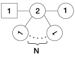
Refer to caption
Refer to caption
Figure 7: New mirror pair obtained from linear quivers Fig. 6. For the quiver on the right there are N1𝑁1N-1 Sp(1)𝑆𝑝1Sp(1) gauge groups in the chain.

Now, let us demonstrate how the gauging procedure may be performed at the level of partition functions. For a generic N𝑁N, the partition function on a round 3-sphere for the A-model is

𝒵A=α=12dsαd2s02!α=12e2πisαηαi=12e2πis0iη0sinh2π(s01s02)i=12coshπ(s1s0i)a=1Ncoshπ(s0i+Ma)coshπ(s2s0i)=d2s02!i=12e2πis0i(t2t3)(e2πis01(t1t2)e2πis02(t1t2))(e2πis01(t3t4)e2πis02(t3t4))4sinhπ(t1t2)sinhπ(t3t4)a=1Ni=12coshπ(s0i+Ma)subscript𝒵𝐴subscriptsuperscriptproduct2𝛼1𝑑subscript𝑠𝛼superscript𝑑2subscript𝑠02subscriptsuperscriptproduct2𝛼1superscript𝑒2𝜋𝑖subscript𝑠𝛼subscript𝜂𝛼subscriptsuperscriptproduct2𝑖1superscript𝑒2𝜋𝑖subscriptsuperscript𝑠𝑖0subscript𝜂0superscript2𝜋subscriptsuperscript𝑠10subscriptsuperscript𝑠20subscriptsuperscriptproduct2𝑖1𝜋subscript𝑠1subscriptsuperscript𝑠𝑖0subscriptsuperscriptproduct𝑁𝑎1𝜋subscriptsuperscript𝑠𝑖0subscript𝑀𝑎𝜋subscript𝑠2subscriptsuperscript𝑠𝑖0superscript𝑑2subscript𝑠02subscriptsuperscriptproduct2𝑖1superscript𝑒2𝜋𝑖subscriptsuperscript𝑠𝑖0subscript𝑡2subscript𝑡3superscript𝑒2𝜋𝑖subscriptsuperscript𝑠10subscript𝑡1subscript𝑡2superscript𝑒2𝜋𝑖subscriptsuperscript𝑠20subscript𝑡1subscript𝑡2superscript𝑒2𝜋𝑖subscriptsuperscript𝑠10subscript𝑡3subscript𝑡4superscript𝑒2𝜋𝑖subscriptsuperscript𝑠20subscript𝑡3subscript𝑡44𝜋subscript𝑡1subscript𝑡2𝜋subscript𝑡3subscript𝑡4subscriptsuperscriptproduct𝑁𝑎1subscriptsuperscriptproduct2𝑖1𝜋subscriptsuperscript𝑠𝑖0subscript𝑀𝑎\begin{split}&{\cal Z}_{A}=\int\prod^{2}_{\alpha=1}ds_{\alpha}\frac{d^{2}s_{0}}{2!}\frac{\prod^{2}_{\alpha=1}e^{2\pi is_{\alpha}\eta_{\alpha}}\prod^{2}_{i=1}e^{2\pi is^{i}_{0}\eta_{0}}\sinh^{2}{\pi(s^{1}_{0}-s^{2}_{0})}}{\prod^{2}_{i=1}\cosh{\pi(s_{1}-s^{i}_{0})}\prod^{N}_{a=1}\cosh{\pi(s^{i}_{0}+M_{a})}\cosh{\pi(s_{2}-s^{i}_{0})}}\\ &=-\int\frac{d^{2}s_{0}}{2!}\frac{\prod^{2}_{i=1}e^{2\pi is^{i}_{0}(t_{2}-t_{3})}\left(e^{2\pi is^{1}_{0}(t_{1}-t_{2})}-e^{2\pi is^{2}_{0}(t_{1}-t_{2})}\right)\left(e^{2\pi is^{1}_{0}(t_{3}-t_{4})}-e^{2\pi is^{2}_{0}(t_{3}-t_{4})}\right)}{4\sinh{\pi(t_{1}-t_{2})}\sinh{\pi(t_{3}-t_{4})}\prod^{N}_{a=1}\prod^{2}_{i=1}\cosh{\pi(s^{i}_{0}+M_{a})}}\end{split} (43)

where we have defined η1=t1t2,η0=t2t3,η2=t3t4formulae-sequencesubscript𝜂1subscript𝑡1subscript𝑡2formulae-sequencesubscript𝜂0subscript𝑡2subscript𝑡3subscript𝜂2subscript𝑡3subscript𝑡4\eta_{1}=t_{1}-t_{2},\eta_{0}=t_{2}-t_{3},\eta_{2}=t_{3}-t_{4}, with the constraint t1+t2+t3+t4=0subscript𝑡1subscript𝑡2subscript𝑡3subscript𝑡40t_{1}+t_{2}+t_{3}+t_{4}=0. The masses obey the constraint a=1NMa=0subscriptsuperscript𝑁𝑎1subscript𝑀𝑎0\sum^{N}_{a=1}M_{a}=0. To obtain the second line, we have simply integrated out the two boundary U(1)𝑈1U(1) nodes in the integral.

The partition function for the B-model (2,2)1(2,0)2(2,0)N2(2,2)N1subscript221subscript202subscript20𝑁2subscript22𝑁1(2,2)_{1}(2,0)_{2}\ldots(2,0)_{N-2}(2,2)_{N-1} is

𝒵B=α=1N1d2sα2!α=1N1i=12e2πisαiη~αsinh2π(sα1sα2)i=12a=12coshπ(s1i+ma)coshπ(sN1i+m¯a)α=1N2i,jcoshπ(sαisα+1j)subscript𝒵𝐵subscriptsuperscriptproduct𝑁1𝛼1superscript𝑑2subscript𝑠𝛼2subscriptsuperscriptproduct𝑁1𝛼1subscriptsuperscriptproduct2𝑖1superscript𝑒2𝜋𝑖subscriptsuperscript𝑠𝑖𝛼subscript~𝜂𝛼superscript2𝜋subscriptsuperscript𝑠1𝛼subscriptsuperscript𝑠2𝛼subscriptsuperscriptproduct2𝑖1subscriptsuperscriptproduct2𝑎1𝜋subscriptsuperscript𝑠𝑖1subscript𝑚𝑎𝜋subscriptsuperscript𝑠𝑖𝑁1subscript¯𝑚𝑎subscriptsuperscriptproduct𝑁2𝛼1subscriptproduct𝑖𝑗𝜋subscriptsuperscript𝑠𝑖𝛼subscriptsuperscript𝑠𝑗𝛼1\begin{split}&{\cal Z}_{B}=\int\prod^{N-1}_{\alpha=1}\frac{d^{2}s_{\alpha}}{2!}\frac{\prod^{N-1}_{\alpha=1}\prod^{2}_{i=1}e^{2\pi is^{i}_{\alpha}\widetilde{\eta}_{\alpha}}\sinh^{2}{\pi(s^{1}_{\alpha}-s^{2}_{\alpha})}}{\prod^{2}_{i=1}\prod^{2}_{a=1}\cosh{\pi(s^{i}_{1}+{m}_{a})}\cosh{\pi(s^{i}_{N-1}+\bar{m}_{a})}\prod^{N-2}_{\alpha=1}\prod_{i,j}\cosh{\pi(s^{i}_{\alpha}-s^{j}_{\alpha+1})}}\end{split} (44)

where we again set η~α=t~αt~α+1subscript~𝜂𝛼subscript~𝑡𝛼subscript~𝑡𝛼1\widetilde{\eta}_{\alpha}=\widetilde{t}_{\alpha}-\widetilde{t}_{\alpha+1} with the constraint α=1Nt~α=0subscriptsuperscript𝑁𝛼1subscript~𝑡𝛼0\sum^{N}_{\alpha=1}\widetilde{t}_{\alpha}=0. As shown in the case for N=2𝑁2N=2, one can show that 𝒵Asubscript𝒵𝐴{\cal Z}_{A} and 𝒵Bsubscript𝒵𝐵{\cal Z}_{B} merely differ by a phase. Using Cauchy determinant formula and the associated tool-box for manipulating S3superscript𝑆3S^{3} partition functions, as explained for example in Dey:2013nf , we obtain,

𝒵B(ma,m¯a;t~α)=e2πit~1(t1+t2)2πit~N(t3+t4)𝒵A(Mα;ti)𝒵A(Mα;ti)=e2πit~1(t1+t2)+2πit~N(t3+t4)𝒵B(ma,m¯a;t~α)subscript𝒵𝐵subscript𝑚𝑎subscript¯𝑚𝑎subscript~𝑡𝛼superscript𝑒2𝜋𝑖subscript~𝑡1subscript𝑡1subscript𝑡22𝜋𝑖subscript~𝑡𝑁subscript𝑡3subscript𝑡4subscript𝒵𝐴subscript𝑀𝛼subscript𝑡𝑖subscript𝒵𝐴subscript𝑀𝛼subscript𝑡𝑖superscript𝑒2𝜋𝑖subscript~𝑡1subscript𝑡1subscript𝑡22𝜋𝑖subscript~𝑡𝑁subscript𝑡3subscript𝑡4subscript𝒵𝐵subscript𝑚𝑎subscript¯𝑚𝑎subscript~𝑡𝛼\begin{split}{\cal Z}_{B}(m_{a},\bar{m}_{a};\widetilde{t}_{\alpha})=&e^{2\pi i\widetilde{t}_{1}(t_{1}+t_{2})-2\pi i\widetilde{t}_{N}(t_{3}+t_{4})}{\cal Z}_{A}(M_{\alpha};t_{i})\\ \implies{\cal Z}_{A}(M_{\alpha};t_{i})=&e^{-2\pi i\widetilde{t}_{1}(t_{1}+t_{2})+2\pi i\widetilde{t}_{N}(t_{3}+t_{4})}{\cal Z}_{B}(m_{a},\bar{m}_{a};\widetilde{t}_{\alpha})\end{split} (45)

The mirror map is simply given by

Mαt~αt1,t2m1,m2t3,t4m¯1,m¯2.subscript𝑀𝛼subscript~𝑡𝛼subscript𝑡1subscript𝑡2subscript𝑚1subscript𝑚2subscript𝑡3subscript𝑡4subscript¯𝑚1subscript¯𝑚2\begin{split}&M_{\alpha}\leftrightarrow\widetilde{t}_{\alpha}\\ &t_{1},t_{2}\leftrightarrow m_{1},m_{2}\\ &t_{3},t_{4}\leftrightarrow\bar{m}_{1},\bar{m}_{2}.\end{split} (46)

One can now gauge the Cartan of the U(N)𝑈𝑁U(N) flavor symmetry labeled by Mα(=t~α)annotatedsubscript𝑀𝛼absentsubscript~𝑡𝛼M_{\alpha}(=\widetilde{t}_{\alpha}) in N𝑁N steps starting with M1(=t~1)annotatedsubscript𝑀1absentsubscript~𝑡1M_{1}(=\widetilde{t}_{1}). As before, in the gauging procedure, we treat the Mα(=t~α)annotatedsubscript𝑀𝛼absentsubscript~𝑡𝛼M_{\alpha}(=\widetilde{t}_{\alpha})s as independent complex parameters without any constraint. Therefore, gauging the first U(1)𝑈1U(1) in the A-model, which in the dual theory corresponds to one of the nodes with fundamental matter, we have

𝒵~A(1)(M2,.MN;ti,η3)=e2πit~N(t3+t4t1t2η3)α=1N1d2sα2!i=12α=2N1e2πisαi(t~αt~α+1)×δ(s11+s12)α=1N1sinh2π(sα1sα2)i=12a=12coshπ(s1i+ta+t1+t2+η32)coshπ(sN1i+t2+a+t1+t2+η32)α=1N2i,jcoshπ(sαisα+1j)\begin{split}&\widetilde{{\cal Z}}^{(1)}_{A}(M_{2},\ldots.M_{N};t_{i},\eta_{3})=e^{2\pi i\widetilde{t}_{N}(t_{3}+t_{4}-t_{1}-t_{2}-\eta_{3})}\int\prod^{N-1}_{\alpha=1}\frac{d^{2}s_{\alpha}}{2!}\prod^{2}_{i=1}\int\prod^{N-1}_{\alpha=2}e^{2\pi is^{i}_{\alpha}\left(\widetilde{t}_{\alpha}-\widetilde{t}_{\alpha+1}\right)}\\ &\times\frac{\delta(s^{1}_{1}+s^{2}_{1})\prod^{N-1}_{\alpha=1}\sinh^{2}{\pi(s^{1}_{\alpha}-s^{2}_{\alpha})}}{\prod^{2}_{i=1}\prod^{2}_{a=1}\cosh{\pi(s^{i}_{1}+{t}_{a}+\frac{t_{1}+t_{2}+\eta_{3}}{2})}\cosh{\pi(s^{i}_{N-1}+{t}_{2+a}+\frac{t_{1}+t_{2}+\eta_{3}}{2})}\prod^{N-2}_{\alpha=1}\prod_{i,j}\cosh{\pi(s^{i}_{\alpha}-s^{j}_{\alpha+1})}}\end{split} (47)

where η3subscript𝜂3\eta_{3} is the FI parameter corresponding to the gauged U(1)𝑈1U(1). The dual theory can be immediately read off from the above partition function - it is the same quiver as the B-model in Fig. 6 with the first U(2)𝑈2U(2) replaced by a Sp(1)𝑆𝑝1Sp(1). The mirror map is also obvious from the above formula- the A-model has (N1)𝑁1(N-1) mass parameters matching the number of remaining t~αsubscript~𝑡𝛼\widetilde{t}_{\alpha} parameters for the B-model. In addition, the 4 independent mass parameters of the B-model are related to the 4 independent FI parameters (tisubscript𝑡𝑖t_{i}s with one constraint and η3subscript𝜂3\eta_{3}) in the A-model in the following fashion:

t~α=Mα(α=2,,N)ma=ta+t1+t2+η32(a=1,2)m¯a=t2+a+t1+t2+η32(a=1,2)subscript~𝑡𝛼subscript𝑀𝛼𝛼2𝑁subscript𝑚𝑎subscript𝑡𝑎subscript𝑡1subscript𝑡2subscript𝜂32𝑎12subscript¯𝑚𝑎subscript𝑡2𝑎subscript𝑡1subscript𝑡2subscript𝜂32𝑎12\begin{split}&\widetilde{t}_{\alpha}=M_{\alpha}\;(\alpha=2,\ldots,N)\\ &m_{a}={t}_{a}+\frac{t_{1}+t_{2}+\eta_{3}}{2}\;(a=1,2)\\ &\bar{m}_{a}={t}_{2+a}+\frac{t_{1}+t_{2}+\eta_{3}}{2}\;(a=1,2)\end{split} (48)

Carrying on with gauging the second U(1)𝑈1U(1), one gets

𝒵~A(2)(M3,.MN;ti,η3,η4)=e2πit~N(t3+t4t1t2η3η4)α=1N1d2sα2!i=12α=3N1e2πisαi(t~αt~α+1)×δ(s11+s12)δ(s21+s22)α=1N1sinh2π(sα1sα2)a,icoshπ(s1i+ta+t1+t2+η32)coshπ(sN1i+t2+a+t1+t2+η3+η42)α=2N2i,jcoshπ(sαisα+1j)×1i,jcoshπ(s1is2jη42)\begin{split}&\widetilde{{\cal Z}}^{(2)}_{A}(M_{3},\ldots.M_{N};t_{i},\eta_{3},\eta_{4})=e^{2\pi i\widetilde{t}_{N}(t_{3}+t_{4}-t_{1}-t_{2}-\eta_{3}-\eta_{4})}\int\prod^{N-1}_{\alpha=1}\frac{d^{2}s_{\alpha}}{2!}\prod^{2}_{i=1}\int\prod^{N-1}_{\alpha=3}e^{2\pi is^{i}_{\alpha}\left(\widetilde{t}_{\alpha}-\widetilde{t}_{\alpha+1}\right)}\\ &\times\frac{\delta(s^{1}_{1}+s^{2}_{1})\delta(s^{1}_{2}+s^{2}_{2})\prod^{N-1}_{\alpha=1}\sinh^{2}{\pi(s^{1}_{\alpha}-s^{2}_{\alpha})}}{\prod_{a,i}\cosh{\pi(s^{i}_{1}+{t}_{a}+\frac{t_{1}+t_{2}+\eta_{3}}{2})}\cosh{\pi(s^{i}_{N-1}+{t}_{2+a}+\frac{t_{1}+t_{2}+\eta_{3}+\eta_{4}}{2})}\prod^{N-2}_{\alpha=2}\prod_{i,j}\cosh{\pi(s^{i}_{\alpha}-s^{j}_{\alpha+1})}}\\ &\times\frac{1}{\prod_{i,j}\cosh{\pi(s^{i}_{1}-s^{j}_{2}-\frac{\eta_{4}}{2})}}\end{split} (49)

The mirror theory is now given by the B-model in Fig. 6 with the first two U(2)𝑈2U(2)s replaced by Sp(1)𝑆𝑝1Sp(1)s and the mirror map in this case can be read off as follows:

t~α=Mα(α=3,,N)ma=ta+t1+t2+η32(a=1,2)m¯a=t2+a+t1+t2+η3+η42(a=1,2)m1bif=η42subscript~𝑡𝛼subscript𝑀𝛼𝛼3𝑁subscript𝑚𝑎subscript𝑡𝑎subscript𝑡1subscript𝑡2subscript𝜂32𝑎12subscript¯𝑚𝑎subscript𝑡2𝑎subscript𝑡1subscript𝑡2subscript𝜂3subscript𝜂42𝑎12subscriptsuperscript𝑚𝑏𝑖𝑓1subscript𝜂42\begin{split}&\widetilde{t}_{\alpha}=M_{\alpha}\;(\alpha=3,\ldots,N)\\ &m_{a}={t}_{a}+\frac{t_{1}+t_{2}+\eta_{3}}{2}\;(a=1,2)\\ &\bar{m}_{a}={t}_{2+a}+\frac{t_{1}+t_{2}+\eta_{3}+\eta_{4}}{2}\;(a=1,2)\\ &m^{bif}_{1}=\frac{\eta_{4}}{2}\end{split} (50)

Note that there is a non-zero mass for the hypermultiplet in the bifundamental representation of Sp(1)×Sp(1)𝑆𝑝1𝑆𝑝1Sp(1)\times Sp(1) in addition to the four fundamental masses. The number of FI parameters in the A-model therefore agrees with the number of mass parameters of the B-model.

Gauging (N1)𝑁1(N-1) of the N𝑁N U(1)𝑈1U(1)s in a manner outlined above, one obtains the desired A-model of Fig. 7 . The resultant partition function

𝒵~A(N1)(MN;ti,η3,η4,,ηN+1)=d2sα2!e2πit~N(t3+t4t1t2η3ηN+1)α=1N2i,jcoshπ(sαisα+1jmαbif)×α=1Nδ(sα1+sα2)α=1N1sinh2π(sα1sα2)a,icoshπ(s1i+ta+t1+t2+η32)coshπ(sN1i+t2+a+t1+t2+η3+η4++ηN+12)subscriptsuperscript~𝒵𝑁1𝐴subscript𝑀𝑁subscript𝑡𝑖subscript𝜂3subscript𝜂4subscript𝜂𝑁1superscript𝑑2subscript𝑠𝛼2superscript𝑒2𝜋𝑖subscript~𝑡𝑁subscript𝑡3subscript𝑡4subscript𝑡1subscript𝑡2subscript𝜂3subscript𝜂𝑁1subscriptsuperscriptproduct𝑁2𝛼1subscriptproduct𝑖𝑗𝜋subscriptsuperscript𝑠𝑖𝛼subscriptsuperscript𝑠𝑗𝛼1subscriptsuperscript𝑚𝑏𝑖𝑓𝛼subscriptsuperscriptproduct𝑁𝛼1𝛿subscriptsuperscript𝑠1𝛼subscriptsuperscript𝑠2𝛼subscriptsuperscriptproduct𝑁1𝛼1superscript2𝜋subscriptsuperscript𝑠1𝛼subscriptsuperscript𝑠2𝛼subscriptproduct𝑎𝑖𝜋subscriptsuperscript𝑠𝑖1subscript𝑡𝑎subscript𝑡1subscript𝑡2subscript𝜂32𝜋subscriptsuperscript𝑠𝑖𝑁1subscript𝑡2𝑎subscript𝑡1subscript𝑡2subscript𝜂3subscript𝜂4subscript𝜂𝑁12\begin{split}&\widetilde{{\cal Z}}^{(N-1)}_{A}(M_{N};t_{i},\eta_{3},\eta_{4},\ldots,\eta_{N+1})=\int\frac{d^{2}s_{\alpha}}{2!}\frac{e^{2\pi i\widetilde{t}_{N}(t_{3}+t_{4}-t_{1}-t_{2}-\eta_{3}-\ldots-\eta_{N+1})}}{\prod^{N-2}_{\alpha=1}\prod_{i,j}\cosh{\pi(s^{i}_{\alpha}-s^{j}_{\alpha+1}-m^{bif}_{\alpha})}}\\ &\times\frac{\prod^{N}_{\alpha=1}\delta(s^{1}_{\alpha}+s^{2}_{\alpha})\prod^{N-1}_{\alpha=1}\sinh^{2}{\pi(s^{1}_{\alpha}-s^{2}_{\alpha})}}{\prod_{a,i}\cosh{\pi(s^{i}_{1}+{t}_{a}+\frac{t_{1}+t_{2}+\eta_{3}}{2})}\cosh{\pi(s^{i}_{N-1}+{t}_{2+a}+\frac{t_{1}+t_{2}+\eta_{3}+\eta_{4}+\ldots+\eta_{N+1}}{2})}}\end{split} (51)

Therefore, up to a field-independent phase, one obtains the expected dual theory of Fig. 7. The masses of the B-model are related to the FI-parameters of the A-model in the following way,

ma=ta+t1+t2+η32(a=1,2)m¯a=t2+a+t1+t2+η3+η4++ηN+12(a=1,2)mαbif=ηα+32(α=1,2,,N2)subscript𝑚𝑎subscript𝑡𝑎subscript𝑡1subscript𝑡2subscript𝜂32𝑎12subscript¯𝑚𝑎subscript𝑡2𝑎subscript𝑡1subscript𝑡2subscript𝜂3subscript𝜂4subscript𝜂𝑁12𝑎12subscriptsuperscript𝑚𝑏𝑖𝑓𝛼subscript𝜂𝛼32𝛼12𝑁2\begin{split}&m_{a}={t}_{a}+\frac{t_{1}+t_{2}+\eta_{3}}{2}\;\;(a=1,2)\\ &\bar{m}_{a}={t}_{2+a}+\frac{t_{1}+t_{2}+\eta_{3}+\eta_{4}+\ldots+\eta_{N+1}}{2}\;\;(a=1,2)\\ &m^{bif}_{\alpha}=\frac{\eta_{\alpha+3}}{2}\;\;(\alpha=1,2,\ldots,N-2)\end{split} (52)

One can further gauge the remaining mass MNsubscript𝑀𝑁M_{N}. The partition function of the gauged theory is

𝒵~A(N)(ti,η3,η4,,ηN+1)=d2sα2!δ(t3t4+t1+t2+η3++ηN+1+ηN+2)α=1N2i,jcoshπ(sαisα+1j)×α=1Nδ(sα1+sα2)α=1N1sinh2π(sα1sα2)a,icoshπ(s1i+ta+t1+t2+η32)coshπ(sN1i+t2+a+t1+t2+η3+η4++ηN+12)subscriptsuperscript~𝒵𝑁𝐴subscript𝑡𝑖subscript𝜂3subscript𝜂4subscript𝜂𝑁1superscript𝑑2subscript𝑠𝛼2𝛿subscript𝑡3subscript𝑡4subscript𝑡1subscript𝑡2subscript𝜂3subscript𝜂𝑁1subscript𝜂𝑁2subscriptsuperscriptproduct𝑁2𝛼1subscriptproduct𝑖𝑗𝜋subscriptsuperscript𝑠𝑖𝛼subscriptsuperscript𝑠𝑗𝛼1subscriptsuperscriptproduct𝑁𝛼1𝛿subscriptsuperscript𝑠1𝛼subscriptsuperscript𝑠2𝛼subscriptsuperscriptproduct𝑁1𝛼1superscript2𝜋subscriptsuperscript𝑠1𝛼subscriptsuperscript𝑠2𝛼subscriptproduct𝑎𝑖𝜋subscriptsuperscript𝑠𝑖1subscript𝑡𝑎subscript𝑡1subscript𝑡2subscript𝜂32𝜋subscriptsuperscript𝑠𝑖𝑁1subscript𝑡2𝑎subscript𝑡1subscript𝑡2subscript𝜂3subscript𝜂4subscript𝜂𝑁12\begin{split}&\widetilde{{\cal Z}}^{(N)}_{A}(t_{i},\eta_{3},\eta_{4},\ldots,\eta_{N+1})=\int\frac{d^{2}s_{\alpha}}{2!}\frac{\delta(-t_{3}-t_{4}+t_{1}+t_{2}+\eta_{3}+\ldots+\eta_{N+1}+\eta_{N+2})}{\prod^{N-2}_{\alpha=1}\prod_{i,j}\cosh{\pi(s^{i}_{\alpha}-s^{j}_{\alpha+1})}}\\ &\times\frac{\prod^{N}_{\alpha=1}\delta(s^{1}_{\alpha}+s^{2}_{\alpha})\prod^{N-1}_{\alpha=1}\sinh^{2}{\pi(s^{1}_{\alpha}-s^{2}_{\alpha})}}{\prod_{a,i}\cosh{\pi(s^{i}_{1}+{t}_{a}+\frac{t_{1}+t_{2}+\eta_{3}}{2})}\cosh{\pi(s^{i}_{N-1}+{t}_{2+a}+\frac{t_{1}+t_{2}+\eta_{3}+\eta_{4}+\ldots+\eta_{N+1}}{2})}}\end{split} (53)

The mirror map remains unchanged. As we saw in the case for N=2𝑁2N=2, gauging the final U(1)𝑈1U(1) imposes an extra constraint on the FI parameters of the A-model, namely

η1+η2+η3++ηN+1+ηN+2+2η0=0.subscript𝜂1subscript𝜂2subscript𝜂3subscript𝜂𝑁1subscript𝜂𝑁22subscript𝜂00\eta_{1}+\eta_{2}+\eta_{3}+\ldots+\eta_{N+1}+\eta_{N+2}+2\eta_{0}=0\,. (54)

The A-model is therefore a Star-shaped quiver with the gauge group U(1)N+2×U(2)//U(1)U(1)^{N+2}\times U(2)//U(1) with U(2)𝑈2U(2) being the central node.

At this point it is easy to propose a higher-rank generalization of the mirror pair from Fig. 7. If we start off with the following linear quiver

(k,k)1(k,0)2(k,0)N2(k,k)N1,subscript𝑘𝑘1subscript𝑘02subscript𝑘0𝑁2subscript𝑘𝑘𝑁1(k,k)_{1}(k,0)_{2}\dots(k,0)_{N-2}\dots(k,k)_{N-1}\,, (55)

then its mirror will be a U(k)𝑈𝑘U(k) theory with N𝑁N flavors and two T[U(k1)]𝑇delimited-[]𝑈𝑘1T[U(k-1)] tails attached to it (see Fig. 8).

Refer to caption
Figure 8: Linear A2k1subscript𝐴2𝑘1A_{2k-1} quiver with two T[U(k1)]𝑇delimited-[]𝑈𝑘1T[U(k-1)] with framing at the middle node which is used to derive the mirror dual for star shaped quivers.

We can now gauge the maximal torus of the U(N)𝑈𝑁U(N) flavor symmetry on the middle node. This gauging imposes a simple constraint on the Cartan of each U(k)𝑈𝑘U(k) gauge group in the dual quiver (55) (and a constraint on the FI parameters if the Cartan of U(N)𝑈𝑁U(N) is fully gauged) which amounts to removing a U(1)𝑈1U(1) subgroup from each U(k)𝑈𝑘U(k) gauge group. This leads us to the mirror pair presented in the first line of Tab. 1.

4.2 Flavorless D^Nsubscript^𝐷𝑁\hat{D}_{N} Quivers

The D^Nsubscript^𝐷𝑁\hat{D}_{N} quiver and its mirror may be obtained by starting from the same pair of linear quivers as we used to obtain the Star-shaped quiver and its mirror dual in Sec. 4.1. The brane constructions of such quivers using ON𝑂superscript𝑁ON^{-} planes are depicted in Fig. 9. In Lindstrom:1999pz several of them are considered and interesting global symmetries of the quivers are discussed.
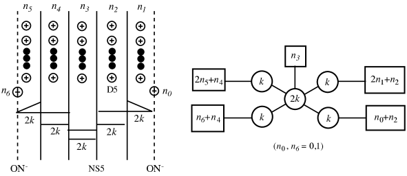
Refer to caption
Figure 9: Brane construction of a generic flavored D^4subscript^𝐷4\hat{D}_{4} quiver. The labels indicate that there are 2k2𝑘2k D3 branes in each interval, i.e.  k𝑘k copies of the D3 branes drawn in the diagram. The numbers n1,,n5subscript𝑛1subscript𝑛5n_{1},\ldots,n_{5} label the numbers of D5-branes at each interval, and the numbers n0,n6=0,1formulae-sequencesubscript𝑛0subscript𝑛601n_{0},n_{6}=0,1 labels the numbers of D5-branes stuck on each ON𝑂superscript𝑁ON^{-} plane.

Start with the following mirror pair of linear quivers (see Fig. 6, with NN2𝑁𝑁2N\to N-2)
A-model: (2,2)1(2,0)2(2,0)N4(2,2)N3subscript221subscript202subscript20𝑁4subscript22𝑁3(2,2)_{1}(2,0)_{2}\ldots(2,0)_{N-4}(2,2)_{N-3}
B-model: (1,0)(2,N2)(1,0)102𝑁210(1,0)(2,N-2)(1,0).

From our computation in the previous section one can readily see that (note that what we called B-model there is the A-model in the present case)

𝒵A(ma,m¯a;t~α)=e2πit~1(t1+t2)2πit~N2(t3+t4)𝒵B(Mα;ti).subscript𝒵𝐴subscript𝑚𝑎subscript¯𝑚𝑎subscript~𝑡𝛼superscript𝑒2𝜋𝑖subscript~𝑡1subscript𝑡1subscript𝑡22𝜋𝑖subscript~𝑡𝑁2subscript𝑡3subscript𝑡4subscript𝒵𝐵subscript𝑀𝛼subscript𝑡𝑖\begin{split}{\cal Z}_{A}(m_{a},\bar{m}_{a};\widetilde{t}_{\alpha})=e^{2\pi i\widetilde{t}_{1}(t_{1}+t_{2})-2\pi i\widetilde{t}_{N-2}(t_{3}+t_{4})}{\cal Z}_{B}(M_{\alpha};t_{i})\,.\end{split} (56)

The mirror map is the same as before and can be read off from the above equation.

Mαt~αt1,t2m1,m2t3,t4m¯1,m¯2.subscript𝑀𝛼subscript~𝑡𝛼subscript𝑡1subscript𝑡2subscript𝑚1subscript𝑚2subscript𝑡3subscript𝑡4subscript¯𝑚1subscript¯𝑚2\begin{split}&M_{\alpha}\leftrightarrow\widetilde{t}_{\alpha}\\ &t_{1},t_{2}\leftrightarrow m_{1},m_{2}\\ &t_{3},t_{4}\leftrightarrow\bar{m}_{1},\bar{m}_{2}.\end{split} (57)

In the example of the Star-shaped quiver, we gauged the U(N)𝑈𝑁U(N) flavor symmetry of the linear quiver (1,0)(2,N)(1,0)102𝑁10(1,0)(2,N)(1,0) as U(1)N𝑈superscript1𝑁U(1)^{N} to obtain the SU(2)×U(1)N𝑆𝑈2𝑈superscript1𝑁SU(2)\times U(1)^{N} Star-shaped quiver. To obtain the D^Nsubscript^𝐷𝑁\hat{D}_{N} quiver, we gauge each of the two U(2)𝑈2U(2) flavor symmetries of the linear quiver (2,2)1(2,0)2(2,0)(2,2)N3subscript221subscript20220subscript22𝑁3(2,2)_{1}(2,0)_{2}\ldots(2,0)(2,2)_{N-3} as U(1)2𝑈superscript12U(1)^{2}. The partition function of the gauged theory is given as

𝒵~A(ζj;t~α)=α=12dsαd2s02!j=14dtje2πiζjtje2πit~1(t1+t2)2πit~N2(t3+t4)e2πis1(t1t2)e2πis2(t3t4)×i=12e2πis0i(t2t3)sinh2π(s01s02)i=12coshπ(s1s0i)a=1N2coshπ(s0i+t~a)coshπ(s2s0i)subscript~𝒵𝐴subscript𝜁𝑗subscript~𝑡𝛼subscriptsuperscriptproduct2𝛼1𝑑subscript𝑠𝛼superscript𝑑2subscript𝑠02subscriptsuperscriptproduct4𝑗1𝑑subscript𝑡𝑗superscript𝑒2𝜋𝑖subscript𝜁𝑗subscript𝑡𝑗superscript𝑒2𝜋𝑖subscript~𝑡1subscript𝑡1subscript𝑡22𝜋𝑖subscript~𝑡𝑁2subscript𝑡3subscript𝑡4superscript𝑒2𝜋𝑖subscript𝑠1subscript𝑡1subscript𝑡2superscript𝑒2𝜋𝑖subscript𝑠2subscript𝑡3subscript𝑡4subscriptsuperscriptproduct2𝑖1superscript𝑒2𝜋𝑖subscriptsuperscript𝑠𝑖0subscript𝑡2subscript𝑡3superscript2𝜋subscriptsuperscript𝑠10subscriptsuperscript𝑠20subscriptsuperscriptproduct2𝑖1𝜋subscript𝑠1subscriptsuperscript𝑠𝑖0subscriptsuperscriptproduct𝑁2𝑎1𝜋subscriptsuperscript𝑠𝑖0subscript~𝑡𝑎𝜋subscript𝑠2subscriptsuperscript𝑠𝑖0\begin{split}\widetilde{{\cal Z}}_{A}(\zeta_{j};\widetilde{t}_{\alpha})=&\int\prod^{2}_{\alpha=1}ds_{\alpha}\frac{d^{2}s_{0}}{2!}\prod^{4}_{j=1}dt_{j}e^{2\pi i\zeta_{j}t_{j}}e^{2\pi i\widetilde{t}_{1}(t_{1}+t_{2})-2\pi i\widetilde{t}_{N-2}(t_{3}+t_{4})}e^{2\pi is_{1}(t_{1}-t_{2})}e^{2\pi is_{2}(t_{3}-t_{4})}\\ &\times\frac{\prod^{2}_{i=1}e^{2\pi is^{i}_{0}(t_{2}-t_{3})}\sinh^{2}{\pi(s^{1}_{0}-s^{2}_{0})}}{\prod^{2}_{i=1}\cosh{\pi(s_{1}-s^{i}_{0})}\prod^{N-2}_{a=1}\cosh{\pi(s^{i}_{0}+\widetilde{t}_{a})}\cosh{\pi(s_{2}-s^{i}_{0})}}\\ \end{split} (58)

Integrating over the tjsubscript𝑡𝑗t_{j}s, we get

𝒵~A(ζj;t~α)=α=12dsαd2s02!δ(s1+ζ1+t~1)δ(s2ζ4+t~N2)δ(s01+s02s1+t~1+ζ2)×δ(s01+s02s2+t~N2ζ3)sinh2π(s01s02)i=12coshπ(s1s0i)a=1N2coshπ(s0i+t~a)coshπ(s2s0i)=d2s02!δ(s01+s02+ζ1+2t~1+ζ2)δ(s01+s02ζ4+2t~N2ζ3)×sinh2π(s01s02)i=12coshπ(s0i+ζ1+t~1)a=1N2coshπ(s0i+t~a)coshπ(s0iζ4+t~N2)subscript~𝒵𝐴subscript𝜁𝑗subscript~𝑡𝛼subscriptsuperscriptproduct2𝛼1𝑑subscript𝑠𝛼superscript𝑑2subscript𝑠02𝛿subscript𝑠1subscript𝜁1subscript~𝑡1𝛿subscript𝑠2subscript𝜁4subscript~𝑡𝑁2𝛿subscriptsuperscript𝑠10subscriptsuperscript𝑠20subscript𝑠1subscript~𝑡1subscript𝜁2𝛿subscriptsuperscript𝑠10subscriptsuperscript𝑠20subscript𝑠2subscript~𝑡𝑁2subscript𝜁3superscript2𝜋subscriptsuperscript𝑠10subscriptsuperscript𝑠20subscriptsuperscriptproduct2𝑖1𝜋subscript𝑠1subscriptsuperscript𝑠𝑖0subscriptsuperscriptproduct𝑁2𝑎1𝜋subscriptsuperscript𝑠𝑖0subscript~𝑡𝑎𝜋subscript𝑠2subscriptsuperscript𝑠𝑖0superscript𝑑2subscript𝑠02𝛿subscriptsuperscript𝑠10subscriptsuperscript𝑠20subscript𝜁12subscript~𝑡1subscript𝜁2𝛿subscriptsuperscript𝑠10subscriptsuperscript𝑠20subscript𝜁42subscript~𝑡𝑁2subscript𝜁3superscript2𝜋subscriptsuperscript𝑠10subscriptsuperscript𝑠20subscriptsuperscriptproduct2𝑖1𝜋subscriptsuperscript𝑠𝑖0subscript𝜁1subscript~𝑡1subscriptsuperscriptproduct𝑁2𝑎1𝜋subscriptsuperscript𝑠𝑖0subscript~𝑡𝑎𝜋subscriptsuperscript𝑠𝑖0subscript𝜁4subscript~𝑡𝑁2\begin{split}\widetilde{{\cal Z}}_{A}(\zeta_{j};\widetilde{t}_{\alpha})=&\int\prod^{2}_{\alpha=1}ds_{\alpha}\frac{d^{2}s_{0}}{2!}\delta(s_{1}+\zeta_{1}+\widetilde{t}_{1})\delta(s_{2}-\zeta_{4}+\widetilde{t}_{N-2})\delta(s^{1}_{0}+s^{2}_{0}-s_{1}+\widetilde{t}_{1}+\zeta_{2})\\ &\times\frac{\delta(s^{1}_{0}+s^{2}_{0}-s_{2}+\widetilde{t}_{N-2}-\zeta_{3})\sinh^{2}{\pi(s^{1}_{0}-s^{2}_{0})}}{\prod^{2}_{i=1}\cosh{\pi(s_{1}-s^{i}_{0})}\prod^{N-2}_{a=1}\cosh{\pi(s^{i}_{0}+\widetilde{t}_{a})}\cosh{\pi(s_{2}-s^{i}_{0})}}\\ =&\int\frac{d^{2}s_{0}}{2!}\delta(s^{1}_{0}+s^{2}_{0}+\zeta_{1}+2\widetilde{t}_{1}+\zeta_{2})\delta(s^{1}_{0}+s^{2}_{0}-\zeta_{4}+2\widetilde{t}_{N-2}-\zeta_{3})\\ &\times\frac{\sinh^{2}{\pi(s^{1}_{0}-s^{2}_{0})}}{\prod^{2}_{i=1}\cosh{\pi(s^{i}_{0}+\zeta_{1}+\widetilde{t}_{1})}\prod^{N-2}_{a=1}\cosh{\pi(s^{i}_{0}+\widetilde{t}_{a})}\cosh{\pi(s^{i}_{0}-\zeta_{4}+\widetilde{t}_{N-2})}}\end{split} (59)

Finally, shifting the integration variables appropriately, we obtain the final form of the partition function for the flavorless D^Nsubscript^𝐷𝑁\hat{D}_{N} quiver.

𝒵~A(ζj;t~α)=δ(ζ1+2t~1+ζ2+ζ42t~N2+ζ3)d2s02!δ(s01+s02)sinh2π(s01s02)×1i=12coshπ(s0i+(ζ1ζ2)2)a=1N2coshπ(s0iζ1+ζ22t~1+t~a)coshπ(s0i+ζ3ζ42)subscript~𝒵𝐴subscript𝜁𝑗subscript~𝑡𝛼𝛿subscript𝜁12subscript~𝑡1subscript𝜁2subscript𝜁42subscript~𝑡𝑁2subscript𝜁3superscript𝑑2subscript𝑠02𝛿subscriptsuperscript𝑠10subscriptsuperscript𝑠20superscript2𝜋subscriptsuperscript𝑠10subscriptsuperscript𝑠201subscriptsuperscriptproduct2𝑖1𝜋subscriptsuperscript𝑠𝑖0subscript𝜁1subscript𝜁22subscriptsuperscriptproduct𝑁2𝑎1𝜋subscriptsuperscript𝑠𝑖0subscript𝜁1subscript𝜁22subscript~𝑡1subscript~𝑡𝑎𝜋subscriptsuperscript𝑠𝑖0subscript𝜁3subscript𝜁42\begin{split}&\widetilde{{\cal Z}}_{A}(\zeta_{j};\widetilde{t}_{\alpha})=\delta(\zeta_{1}+2\widetilde{t}_{1}+\zeta_{2}+\zeta_{4}-2\widetilde{t}_{N-2}+\zeta_{3})\int\frac{d^{2}s_{0}}{2!}\delta(s^{1}_{0}+s^{2}_{0})\sinh^{2}{\pi(s^{1}_{0}-s^{2}_{0})}\\ &\times\frac{1}{\prod^{2}_{i=1}\cosh{\pi(s^{i}_{0}+\frac{(\zeta_{1}-\zeta_{2})}{2})}\prod^{N-2}_{a=1}\cosh{\pi(s^{i}_{0}-\frac{\zeta_{1}+\zeta_{2}}{2}-\widetilde{t}_{1}+\widetilde{t}_{a})}\cosh{\pi(s^{i}_{0}+\frac{\zeta_{3}-\zeta_{4}}{2})}}\end{split} (60)

The delta function indicates that there exists one constraint involving FI parameters of the D^Nsubscript^𝐷𝑁\hat{D}_{N} quiver, which is equivalent to saying that an overall U(1)𝑈1U(1) factor decouples from the gauge group. Note that this should be taken as part of the definition of the flavorless D^Nsubscript^𝐷𝑁\hat{D}_{N} quiver. Explicitly, the constraint can be written as,

ζ1+ζ2+ζ3+ζ4+2t~12t~N2=0i=14ζi+2j=1N3η~j=0.subscript𝜁1subscript𝜁2subscript𝜁3subscript𝜁42subscript~𝑡12subscript~𝑡𝑁20subscriptsuperscript4𝑖1subscript𝜁𝑖2subscriptsuperscript𝑁3𝑗1subscript~𝜂𝑗0\zeta_{1}+\zeta_{2}+\zeta_{3}+\zeta_{4}+2\widetilde{t}_{1}-2\widetilde{t}_{N-2}=0\Leftrightarrow\sum^{4}_{i=1}\zeta_{i}+2\sum^{N-3}_{j=1}\widetilde{\eta}_{j}=0\,. (61)

The constraint is again of the form iηili=0subscript𝑖subscript𝜂𝑖subscript𝑙𝑖0\sum_{i}\eta_{i}l_{i}=0 - where the sum runs over all the nodes of the quiver and lisubscript𝑙𝑖l_{i} denotes the Dynkin label of the i𝑖i-th node. Taken with the other constraint ata=0subscript𝑎subscript𝑡𝑎0\sum_{a}t_{a}=0, this tells us that there are exactly N𝑁N independent FI parameters - N+2𝑁2N+2 parameters with 2 constraints.
The mirror dual of the D^Nsubscript^𝐷𝑁\hat{D}_{N} quiver so defined, can now be read off from the partition function of the theory – it is a Sp(1)𝑆𝑝1Sp(1) gauge theory with N𝑁N fundamental hypers. The mirror map relating the N𝑁N masses to the FI parameters of the D^Nsubscript^𝐷𝑁\hat{D}_{N} quiver is

M1=ζ2ζ12Ma=ζ1+ζ22+t~1t~a(a=1,2,3,,N2)MN=ζ4ζ32subscript𝑀1subscript𝜁2subscript𝜁12subscript𝑀𝑎subscript𝜁1subscript𝜁22subscript~𝑡1subscript~𝑡𝑎𝑎123𝑁2subscript𝑀𝑁subscript𝜁4subscript𝜁32\begin{split}&M_{1}=\frac{\zeta_{2}-\zeta_{1}}{2}\\ &M_{a}=\frac{\zeta_{1}+\zeta_{2}}{2}+\widetilde{t}_{1}-\widetilde{t}_{a}\;\;(a=1,2,3,\ldots,N-2)\\ &M_{N}=\frac{\zeta_{4}-\zeta_{3}}{2}\end{split} (62)

Therefore the Abelian gauging technique allows one to derive the D^Nsubscript^𝐷𝑁\hat{D}_{N} quiver and its mirror from a pair of mirror dual linear quivers.

4.3 D^Nsubscript^𝐷𝑁\hat{D}_{N} Quivers with Single Framing

Let us start analyzing quivers with framing. For framed D^Nsubscript^𝐷𝑁\hat{D}_{N} quivers there are two obvious cases which require separate analysis: a framed node on the bifurcated edge of the quiver or a framed internal node. We look at both cases below.

4.3.1 Framing on an internal node

In order to obtain a generic mirror pair in this class by Abelian gauging, we start from the following linear quivers (Fig. 10)

Refer to caption
Figure 10: A-model (2,2)1(2,0)2(2,0)N4(2,2)N3(1,0)N2subscript221subscript202subscript20𝑁4subscript22𝑁3subscript10𝑁2(2,2)_{1}(2,0)_{2}\ldots(2,0)_{N-4}(2,2)_{N-3}(1,0)_{N-2} and B-model (1,0)(2,N3)(2,2)102𝑁322(1,0)(2,N-3)(2,2).

There is however a special case when N=4𝑁4N=4 – the A-model quiver looks slightly different (see Fig. 11) in this case.

Refer to caption
Figure 11: A-model (2,4)(1,0)2410(2,4)(1,0) and B-model (1,0)(2,1)(2,2)102122(1,0)(2,1)(2,2).

The partition functions of two linear quivers from (10) are related in the following way

𝒵A(ma;t~α)=e2πit~1(m1+m2m3)2πit~N2(m3m4)2πit~N1m4𝒵B(Mα;ta),subscript𝒵𝐴subscript𝑚𝑎subscript~𝑡𝛼superscript𝑒2𝜋𝑖subscript~𝑡1subscript𝑚1subscript𝑚2subscript𝑚32𝜋𝑖subscript~𝑡𝑁2subscript𝑚3subscript𝑚42𝜋𝑖subscript~𝑡𝑁1subscript𝑚4subscript𝒵𝐵subscript𝑀𝛼subscript𝑡𝑎\begin{split}{\cal Z}_{A}(m_{a};\widetilde{t}_{\alpha})=e^{2\pi i\widetilde{t}_{1}(m_{1}+m_{2}-m_{3})-2\pi i\widetilde{t}_{N-2}(m_{3}-m_{4})-2\pi i\widetilde{t}_{N-1}m_{4}}{\cal Z}_{B}(M_{\alpha};t_{a})\,,\end{split} (63)

where a=1,2,3,4;α=1,2,,N1formulae-sequence𝑎1234𝛼12𝑁1a=1,2,3,4;\;\alpha=1,2,\ldots,N-1. The mirror map can be read off from the above equation.

Mα=t~α,ta=ma.formulae-sequencesubscript𝑀𝛼subscript~𝑡𝛼subscript𝑡𝑎subscript𝑚𝑎\begin{split}&M_{\alpha}=\widetilde{t}_{\alpha}\,,\\ &t_{a}=m_{a}\,.\end{split} (64)

In order to obtain the appropriate D^Nsubscript^𝐷𝑁\hat{D}_{N} quiver, one has to gauge the Cartan of the U(2)1𝑈subscript21U(2)_{1} flavor symmetry (parametrized by m1,m2subscript𝑚1subscript𝑚2m_{1},m_{2}) and partially gauge the Cartan of U(2)N3𝑈subscript2𝑁3U(2)_{N-3} (parametrized by m3,m4subscript𝑚3subscript𝑚4m_{3},m_{4}). One can carry out the gauging one U(1)𝑈1U(1) at a time and at each step one obtains a new family of mirror pairs.

Step 1: Gauging m1subscript𝑚1m_{1}

The mirror pair obtained by gauging m1subscript𝑚1m_{1} is given in Fig. 12.

Refer to caption
Figure 12: A-model (1,0)(2,1)1(2,0)2(2,2)N3(1,0)N210subscript211subscript202subscript22𝑁3subscript10𝑁2(1,0)(2,1)_{1}(2,0)_{2}\ldots(2,2)_{N-3}(1,0)_{N-2} and B-model (2,N2)(2,2)2𝑁222(2,N-2)(2,2).

On the A side we gauged U(1)U(2)𝑈1𝑈2U(1)\subset U(2) of the global symmetry on the first node, thereby enlarging the A-quiver by (1,0)10(1,0) node. On the B-side the U(1)𝑈1U(1) factor got “ungauged” and become a global symmetry on the second node which resulted in the increase of the rank of the corresponding global symmetry group.

The partition functions of the two theories are related in the following fashion

𝒵~A(1)(ma;t~α,ζ1)=e2πim2(ζ1+2t~1)e2πit~1m32πit~N2(m3m4)2πit~N1m4𝒵~B(2)(Mβ;ta)subscriptsuperscript~𝒵1𝐴subscript𝑚𝑎subscript~𝑡𝛼subscript𝜁1superscript𝑒2𝜋𝑖subscript𝑚2subscript𝜁12subscript~𝑡1superscript𝑒2𝜋𝑖subscript~𝑡1subscript𝑚32𝜋𝑖subscript~𝑡𝑁2subscript𝑚3subscript𝑚42𝜋𝑖subscript~𝑡𝑁1subscript𝑚4subscriptsuperscript~𝒵2𝐵subscript𝑀𝛽subscript𝑡𝑎\begin{split}\widetilde{{\cal Z}}^{(1)}_{A}(m_{a};\widetilde{t}_{\alpha},\zeta_{1})=e^{2\pi im_{2}(\zeta_{1}+2\widetilde{t}_{1})}e^{-2\pi i\widetilde{t}_{1}m_{3}-2\pi i\widetilde{t}_{N-2}(m_{3}-m_{4})-2\pi i\widetilde{t}_{N-1}m_{4}}\widetilde{{\cal Z}}^{(2)}_{B}(M_{\beta};t_{a})\end{split} (65)

where a=2,3,4𝑎234a=2,3,4, α=1,2,,N1𝛼12𝑁1\alpha=1,2,\ldots,N-1 and β=1,2,,N𝛽12𝑁\beta=1,2,\ldots,N. Here, ζ1subscript𝜁1\zeta_{1} corresponds to the FI parameter of the newly introduced U(1)𝑈1U(1) node.
The mirror map can be read off from the above equation as before.

Mα=t~αMN=ζ1+t~1ta=masubscript𝑀𝛼subscript~𝑡𝛼subscript𝑀𝑁subscript𝜁1subscript~𝑡1subscript𝑡𝑎subscript𝑚𝑎\begin{split}&M_{\alpha}=\widetilde{t}_{\alpha}\\ &M_{N}=\zeta_{1}+\widetilde{t}_{1}\\ &t_{a}=m_{a}\end{split} (66)

Step 2: Gauging m2subscript𝑚2m_{2}

Next we gauge the remaining global U(1)𝑈1U(1) on the second node of the A-quiver (Fig. 13) as a result of which the associated U(2)𝑈2U(2) gauge group is partially “ungauged” to an Sp(1)𝑆𝑝1Sp(1).

Refer to caption
Figure 13: A-model (1,0)2(2,0)1(2,0)2(2,0)N4(2,2)N3(1,0)N2superscript102subscript201subscript202subscript20𝑁4subscript22𝑁3subscript10𝑁2(1,0)^{2}(2,0)_{1}(2,0)_{2}\ldots(2,0)_{N-4}(2,2)_{N-3}(1,0)_{N-2} and B-model (Sp(1),N2)(2,2)𝑆𝑝1𝑁222(Sp(1),N-2)(2,2).

The partition functions of the two theories are related in the following fashion

𝒵~A(2)(ma;t~α,ζ1,ζ2)=e2πi(t~1+t~N2)m3e2πi(ζ1+ζ2+2t~1t~N2t~N1)m4𝒵~B(2)(Mβ;ta)subscriptsuperscript~𝒵2𝐴subscript𝑚𝑎subscript~𝑡𝛼subscript𝜁1subscript𝜁2superscript𝑒2𝜋𝑖subscript~𝑡1subscript~𝑡𝑁2subscript𝑚3superscript𝑒2𝜋𝑖subscript𝜁1subscript𝜁22subscript~𝑡1subscript~𝑡𝑁2subscript~𝑡𝑁1subscript𝑚4subscriptsuperscript~𝒵2𝐵subscript𝑀𝛽subscript𝑡𝑎\begin{split}\widetilde{{\cal Z}}^{(2)}_{A}(m_{a};\widetilde{t}_{\alpha},\zeta_{1},\zeta_{2})=e^{2\pi i(-\widetilde{t}_{1}+\widetilde{t}_{N-2})m_{3}}e^{2\pi i(\zeta_{1}+\zeta_{2}+2\widetilde{t}_{1}-\widetilde{t}_{N-2}-\widetilde{t}_{N-1})m_{4}}\widetilde{{\cal Z}}^{(2)}_{B}(M_{\beta};t_{a})\end{split} (67)

where a=3,4𝑎34a=3,4, α=1,2,,N1𝛼12𝑁1\alpha=1,2,\ldots,N-1 and β=1,2,,N𝛽12𝑁\beta=1,2,\ldots,N. Here, ζ2subscript𝜁2\zeta_{2} corresponds to the FI parameter of the newly introduced U(1)𝑈1U(1) node.
The mirror map can be read off from the above equation as before.

Mα=ζ1+ζ22+t~1t~α,a=1,2,,N1MN=ζ2ζ12t3=m3,t4=m4.formulae-sequenceformulae-sequencesubscript𝑀𝛼subscript𝜁1subscript𝜁22subscript~𝑡1subscript~𝑡𝛼formulae-sequence𝑎12𝑁1subscript𝑀𝑁subscript𝜁2subscript𝜁12subscript𝑡3subscript𝑚3subscript𝑡4subscript𝑚4\begin{split}&M_{\alpha}=\frac{\zeta_{1}+\zeta_{2}}{2}+\widetilde{t}_{1}-\widetilde{t}_{\alpha},\;a=1,2,\ldots,N-1\\ &M_{N}=\frac{\zeta_{2}-\zeta_{1}}{2}\\ &t_{3}=m_{3},\;t_{4}=m_{4}\,.\end{split} (68)

Step 3: Gauging m3subscript𝑚3m_{3}

Finally we gauge U(1)U(2)𝑈1𝑈2U(1)\subset U(2) on the second node from the right of the A-quiver to obtain the desired framed D^Nsubscript^𝐷𝑁\hat{D}_{N} quiver and the Sp-SO-type quiver on the mirror side (Fig. 14).

Refer to caption
Figure 14: A-model D^Nsubscript^𝐷𝑁\hat{D}_{N} quiver with labels (1,0)2(2,0)1(2,0)2(2,1)N3(1,0)2superscript102subscript201subscript202subscript21𝑁3superscript102(1,0)^{2}(2,0)_{1}(2,0)_{2}\ldots(2,1)_{N-3}(1,0)^{2} and B-model (Sp(1),N2)(Sp(1),2)𝑆𝑝1𝑁2𝑆𝑝12(Sp(1),N-2)(Sp(1),2).

For N=4𝑁4N=4, the mirror pair specified above is exactly the one in Fig. 15. The partition functions of the two theories are related in the following fashion

𝒵~A(3)(m4;t~α,ζ1,ζ2,ζ3)=e2πi(ζ1+ζ2+ζ3+t~1t~N1)m4𝒵~B(3)(Mβ,mbif;t4)subscriptsuperscript~𝒵3𝐴subscript𝑚4subscript~𝑡𝛼subscript𝜁1subscript𝜁2subscript𝜁3superscript𝑒2𝜋𝑖subscript𝜁1subscript𝜁2subscript𝜁3subscript~𝑡1subscript~𝑡𝑁1subscript𝑚4subscriptsuperscript~𝒵3𝐵subscript𝑀𝛽subscript𝑚𝑏𝑖𝑓subscript𝑡4\begin{split}\widetilde{{\cal Z}}^{(3)}_{A}(m_{4};\widetilde{t}_{\alpha},\zeta_{1},\zeta_{2},\zeta_{3})=e^{2\pi i(\zeta_{1}+\zeta_{2}+\zeta_{3}+\widetilde{t}_{1}-\widetilde{t}_{N-1})m_{4}}\widetilde{{\cal Z}}^{(3)}_{B}(M_{\beta},m_{bif};t_{4})\end{split} (69)

where α=1,2,,N1𝛼12𝑁1\alpha=1,2,\ldots,N-1 and β=1,2,,N𝛽12𝑁\beta=1,2,\ldots,N. Here, ζ3subscript𝜁3\zeta_{3} corresponds to the FI parameter of the newly introduced U(1)𝑈1U(1) node. mbifsubscript𝑚𝑏𝑖𝑓m_{bif} is a non-zero mass parameter for the Sp(1)×Sp(1)𝑆𝑝1𝑆𝑝1Sp(1)\times Sp(1) bi-fundamental hyper.
The mirror map can be read off from the above equation as before.

Mα=ζ1+ζ22+t~1t~α,α=1,2,,N3MN2=ζ2ζ12MN1=ζ1+ζ2+ζ32+t~1t~N22MN=ζ1+ζ2+ζ32+t~1+t~N22t~N12mbif=t~1t~N2ζ32t4=m4formulae-sequencesubscript𝑀𝛼subscript𝜁1subscript𝜁22subscript~𝑡1subscript~𝑡𝛼formulae-sequence𝛼12𝑁3subscript𝑀𝑁2subscript𝜁2subscript𝜁12subscript𝑀𝑁1subscript𝜁1subscript𝜁2subscript𝜁32subscript~𝑡1subscript~𝑡𝑁22subscript𝑀𝑁subscript𝜁1subscript𝜁2subscript𝜁32subscript~𝑡1subscript~𝑡𝑁22subscript~𝑡𝑁12subscript𝑚𝑏𝑖𝑓subscript~𝑡1subscript~𝑡𝑁2subscript𝜁32subscript𝑡4subscript𝑚4\begin{split}&M_{\alpha}=\frac{\zeta_{1}+\zeta_{2}}{2}+\widetilde{t}_{1}-\widetilde{t}_{\alpha},\;\alpha=1,2,\ldots,N-3\\ &M_{N-2}=\frac{\zeta_{2}-\zeta_{1}}{2}\\ &M_{N-1}=\frac{\zeta_{1}+\zeta_{2}+\zeta_{3}}{2}+\frac{\widetilde{t}_{1}-\widetilde{t}_{N-2}}{2}\\ &M_{N}=\frac{\zeta_{1}+\zeta_{2}+\zeta_{3}}{2}+\frac{\widetilde{t}_{1}+\widetilde{t}_{N-2}-2\widetilde{t}_{N-1}}{2}\\ &m_{bif}=\frac{\widetilde{t}_{1}-\widetilde{t}_{N-2}-\zeta_{3}}{2}\\ &t_{4}=m_{4}\end{split} (70)

Note that the number of independent FI parameters for the A-model is N+1𝑁1N+1, namely N1𝑁1N-1 parameters {t~α}subscript~𝑡𝛼\{\widetilde{t}_{\alpha}\} with one constraint and three ζisubscript𝜁𝑖\zeta_{i}. This exactly matches with the number of mass parameters of the B-model, namely N𝑁N fundamental masses and one bi-fundamental mass.

Obviously, one can go ahead and gauge the remaining U(1)𝑈1U(1) as well. As we saw in the previous section, this does not change the mirror map in any way but imposes a constraint on the FI parameters of the A-model which is tantamount to having an overall U(1)𝑈1U(1) factor decouple from the gauge group. More explicitly, the mirror pair in this case is the following
A-model: (1,0)2(2,0)1(2,0)2(2,1)N3(1,0)3//U(1)(1,0)^{2}(2,0)_{1}(2,0)_{2}\ldots(2,1)_{N-3}(1,0)^{3}//U(1)
B-model: (Sp(1),N2)(Sp(1),2)𝑆𝑝1𝑁2𝑆𝑝12(Sp(1),N-2)(Sp(1),2).

Refer to caption
Figure 15: Framed D^4subscript^𝐷4\hat{D}_{4} quiver on the left and its mirror on the right. The Higgs branch of quiver (a) is the moduli space of k𝑘k SU(2)𝑆𝑈2SU(2) instantons on 2/D^4superscript2subscript^𝐷4\mathbb{C}^{2}/\hat{D}_{4} and that of quiver (b) corresponds to k𝑘k SO(8)𝑆𝑂8SO(8) instantons on 2/2superscript2subscript2\mathbb{C}^{2}/\mathbb{Z}_{2}.

A generic D^Nsubscript^𝐷𝑁\hat{D}_{N} quiver with a framing in this class (see Fig. 15 for N=4𝑁4N=4) and gauge groups of arbitrary rank as well as its mirror dual can be derived by starting from the following linear quivers:
A-model: (2k,2k)1(2k,0)2(2k,0)3(2k,k+1)N3(k,0)subscript2𝑘2𝑘1subscript2𝑘02subscript2𝑘03subscript2𝑘𝑘1𝑁3𝑘0(2k,2k)_{1}(2k,0)_{2}(2k,0)_{3}\ldots(2k,k+1)_{N-3}(k,0)
B-model: (1,0)(2,0)(2k1,0)(2k,N3)(2k,2)(2k2)(4,0)(2,0)10202𝑘102𝑘𝑁32𝑘22𝑘24020(1,0)(2,0)\ldots(2k-1,0)(2k,N-3)(2k,2)(2k-2)\ldots(4,0)(2,0)
To obtain the appropriate D^Nsubscript^𝐷𝑁\hat{D}_{N} quiver, one needs to completely gauge the U(2k)𝑈2𝑘U(2k) flavor group as U(k)×U(k)𝑈𝑘𝑈𝑘U(k)\times U(k), while for the U(k+1)𝑈𝑘1U(k+1) flavor group, a U(k)𝑈𝑘U(k) subgroup should be gauged.

4.3.2 Framing on boundary nodes

Let us proceed with D^4subscript^𝐷4\hat{D}_{4} quiver, this time with a single hypermultiplet at a boundary node (like quiver (a) in Fig. 16).

Refer to caption
Figure 16: Single framed D^4subscript^𝐷4\hat{D}_{4} quiver and its mirror. The Higgs branch of quiver (a) is the moduli space of k𝑘k U(1)𝑈1U(1) instantons on 2/D^4superscript2subscript^𝐷4\mathbb{C}^{2}/\hat{D}_{4} and that of quiver (b) corresponds to k𝑘k SO(8)𝑆𝑂8SO(8) instantons on 2superscript2\mathbb{C}^{2}. On the right quiver ‘A’ stands for the (reducible) antisymmetric representation of Sp(k)𝑆𝑝𝑘Sp(k).

In order to derive a mirror for this quiver by Abelian gauging, we start from the following linear quivers – A-model with labels (1,0)(2,2)(1,1)102211(1,0)(2,2)(1,1) and B-model with labels (1,1)(2,3)1123(1,1)(2,3) (see Fig. 17).

Refer to caption
Refer to caption
Figure 17: Two mirror dual linear quivers which give rise to mirror pair in Fig. 16.

We perform the abelian gauging trick on the U(2)𝑈2U(2) flavor symmetry on the second node of the left quiver in Fig. 17 in order to map it onto the A model quiver in Fig. 16. Let us see what happens with its mirror. The dimensions of the Coulomb and Higgs branches on the A-model quiver are 444 and 333 respectively. After the gauging is done they become 666 and 111 correspondingly. In the classical parameter space description, this happens because two momenta pμasuperscriptsubscript𝑝𝜇𝑎p_{\mu}^{a} on the A-model quiver get fixed, and two more vectormultiplets are introduced. Thus on the B side the dimension of the Coulomb branch has to drop by two. We can see that this indeed happens if we multiply two Bethe equations for the two gauge nodes of the B quiver. Because of the mirror constraints on pτjsuperscriptsubscript𝑝𝜏𝑗p_{\tau}^{\vee\,j} the value of σ(2)superscript𝜎2\sigma^{(2)} is fixed by pτ 3superscriptsubscript𝑝𝜏3p_{\tau}^{\vee\,3}. The second mirror constraint provides the projection of U(2)Sp(1)𝑈2𝑆𝑝1U(2)\to Sp(1) via σ1(1)σ2(1)=1subscriptsuperscript𝜎11subscriptsuperscript𝜎121\sigma^{\vee\,(1)}_{1}\sigma^{\vee\,(1)}_{2}=1, which can be implemented by adjusting the momenta and twists. Notice that classical analysis does not explicitly show the contribution of the singlet multiplet A in Fig. 16.

In order to see how abelian gauging leads to the mirror pair we want and in particular how antisymmetric matter (a singlet when k=1𝑘1k=1) appears in the mirror we perform gauging of the linear quivers using the partition function approach. For the two linear quivers from Fig. 17 the partition functions are

𝒵A(ma;tα)=α=12dsαd2s02!α=12e2πisαηαi=12e2πis0iη0sinh2π(s01s02)i=12coshπ(s1s0i)a=12coshπ(s0i+ma)coshπ(s2s0i)×1coshπ(s2+m3),𝒵B(Mα;t~a)=𝑑s1d2s02!e2πis1η~1i=12e2πis0iη~0sinh2π(s01s02)i=12coshπ(s0is1)a=13coshπ(s0i+Ma)coshπ(s1+M4),formulae-sequencesubscript𝒵𝐴subscript𝑚𝑎subscript𝑡𝛼subscriptsuperscriptproduct2𝛼1𝑑subscript𝑠𝛼superscript𝑑2subscript𝑠02subscriptsuperscriptproduct2𝛼1superscript𝑒2𝜋𝑖subscript𝑠𝛼subscript𝜂𝛼subscriptsuperscriptproduct2𝑖1superscript𝑒2𝜋𝑖subscriptsuperscript𝑠𝑖0subscript𝜂0superscript2𝜋subscriptsuperscript𝑠10subscriptsuperscript𝑠20subscriptsuperscriptproduct2𝑖1𝜋subscript𝑠1subscriptsuperscript𝑠𝑖0subscriptsuperscriptproduct2𝑎1𝜋subscriptsuperscript𝑠𝑖0subscript𝑚𝑎𝜋subscript𝑠2subscriptsuperscript𝑠𝑖01𝜋subscript𝑠2subscript𝑚3subscript𝒵𝐵subscript𝑀𝛼subscript~𝑡𝑎differential-dsubscript𝑠1superscript𝑑2subscript𝑠02superscript𝑒2𝜋𝑖subscript𝑠1subscript~𝜂1subscriptsuperscriptproduct2𝑖1superscript𝑒2𝜋𝑖subscriptsuperscript𝑠𝑖0subscript~𝜂0superscript2𝜋subscriptsuperscript𝑠10subscriptsuperscript𝑠20subscriptsuperscriptproduct2𝑖1𝜋subscriptsuperscript𝑠𝑖0subscript𝑠1subscriptsuperscriptproduct3𝑎1𝜋subscriptsuperscript𝑠𝑖0subscript𝑀𝑎𝜋subscript𝑠1subscript𝑀4\begin{split}{\cal Z}_{A}(m_{a};{t}_{\alpha})=&\int\prod^{2}_{\alpha=1}ds_{\alpha}\frac{d^{2}s_{0}}{2!}\frac{\prod^{2}_{\alpha=1}e^{2\pi is_{\alpha}\eta_{\alpha}}\prod^{2}_{i=1}e^{2\pi is^{i}_{0}\eta_{0}}\sinh^{2}{\pi(s^{1}_{0}-s^{2}_{0})}}{\prod^{2}_{i=1}\cosh{\pi(s_{1}-s^{i}_{0})}\prod^{2}_{a=1}\cosh{\pi(s^{i}_{0}+m_{a})}\cosh{\pi(s_{2}-s^{i}_{0})}}\\ &\times\frac{1}{\cosh{\pi(s_{2}+m_{3})}}\,,\\ {\cal Z}_{B}(M_{\alpha};\widetilde{t}_{a})=&\int ds_{1}\frac{d^{2}s_{0}}{2!}\frac{e^{2\pi is_{1}\widetilde{\eta}_{1}}\prod^{2}_{i=1}e^{2\pi is^{i}_{0}\widetilde{\eta}_{0}}\sinh^{2}{\pi(s^{1}_{0}-s^{2}_{0})}}{\prod^{2}_{i=1}\cosh{\pi(s^{i}_{0}-s_{1})}\prod^{3}_{a=1}\cosh{\pi(s^{i}_{0}+M_{a})}\cosh{\pi(s_{1}+M_{4})}}\,,\end{split} (71)

where a=1,2,3,4;α=1,2,,N1formulae-sequence𝑎1234𝛼12𝑁1a=1,2,3,4;\;\alpha=1,2,\ldots,N-1. In the A-model, the FI parameters are defined as η1=t1t2,η0=t2t3,η2=t3t4formulae-sequencesubscript𝜂1subscript𝑡1subscript𝑡2formulae-sequencesubscript𝜂0subscript𝑡2subscript𝑡3subscript𝜂2subscript𝑡3subscript𝑡4\eta_{1}=t_{1}-t_{2},\eta_{0}=t_{2}-t_{3},\eta_{2}=t_{3}-t_{4}, while for the B-model, these are η~0=t~1t~2,η~1=t~2t~3formulae-sequencesubscript~𝜂0subscript~𝑡1subscript~𝑡2subscript~𝜂1subscript~𝑡2subscript~𝑡3\widetilde{\eta}_{0}=\widetilde{t}_{1}-\widetilde{t}_{2},\widetilde{\eta}_{1}=\widetilde{t}_{2}-\widetilde{t}_{3}.

The mirror symmetry implies that 𝒵A(ma;tα)=𝒵B(Mα;t~a)subscript𝒵𝐴subscript𝑚𝑎subscript𝑡𝛼subscript𝒵𝐵subscript𝑀𝛼subscript~𝑡𝑎{\cal Z}_{A}(m_{a};{t}_{\alpha})={\cal Z}_{B}(M_{\alpha};\widetilde{t}_{a}) up to some overall phase (which we shall ignore in this example and the subsequent ones) provided the parameters are related as follows:

Mα=tαt~a=ma.subscript𝑀𝛼subscript𝑡𝛼subscript~𝑡𝑎subscript𝑚𝑎\begin{split}&M_{\alpha}={t}_{\alpha}\\ &\widetilde{t}_{a}=m_{a}\,.\end{split} (72)

Now, we gauge the U(2)𝑈2U(2) flavor symmetry of the A-model as a U(1)×U(1)𝑈1𝑈1U(1)\times U(1), which gives a D^4subscript^𝐷4\hat{D}_{4} quiver with a single flavor on one of the boundary nodes. The partition function of this theory is

𝒵~A(ζ1,ζ2,m3;tα)=𝑑m1𝑑m2e2πim1ζ1e2πim2ζ2𝒵A(ma;tα)=𝑑m1𝑑m2e2πim1ζ1e2πim2ζ2𝒵B(tα;ma),subscript~𝒵𝐴subscript𝜁1subscript𝜁2subscript𝑚3subscript𝑡𝛼differential-dsubscript𝑚1differential-dsubscript𝑚2superscript𝑒2𝜋𝑖subscript𝑚1subscript𝜁1superscript𝑒2𝜋𝑖subscript𝑚2subscript𝜁2subscript𝒵𝐴subscript𝑚𝑎subscript𝑡𝛼differential-dsubscript𝑚1differential-dsubscript𝑚2superscript𝑒2𝜋𝑖subscript𝑚1subscript𝜁1superscript𝑒2𝜋𝑖subscript𝑚2subscript𝜁2subscript𝒵𝐵subscript𝑡𝛼subscript𝑚𝑎\begin{split}\widetilde{{\cal Z}}_{A}(\zeta_{1},\zeta_{2},m_{3};{t}_{\alpha})=&\int dm_{1}dm_{2}e^{2\pi im_{1}\zeta_{1}}e^{2\pi im_{2}\zeta_{2}}{\cal Z}_{A}(m_{a};{t}_{\alpha})\\ =&\int dm_{1}dm_{2}e^{2\pi im_{1}\zeta_{1}}e^{2\pi im_{2}\zeta_{2}}{\cal Z}_{B}(t_{\alpha};m_{a})\,,\end{split} (73)

where the second equality follows from the mirror symmetry of the linear quivers. From the second equality, completing the integration over m1subscript𝑚1m_{1} and m2subscript𝑚2m_{2} we have

𝒵~A(ζ1,ζ2,m3;tα)=𝑑s1d2s02!δ(s01+s02+ζ1)δ(s01s02+s1+ζ2)sinh2π(s01s02)iα=13coshπ(s0i+tα)×e2πim3s1icoshπ(s0is1)coshπ(s1+t4).subscript~𝒵𝐴subscript𝜁1subscript𝜁2subscript𝑚3subscript𝑡𝛼differential-dsubscript𝑠1superscript𝑑2subscript𝑠02𝛿subscriptsuperscript𝑠10subscriptsuperscript𝑠20subscript𝜁1𝛿subscriptsuperscript𝑠10subscriptsuperscript𝑠20subscript𝑠1subscript𝜁2superscript2𝜋subscriptsuperscript𝑠10subscriptsuperscript𝑠20subscriptproduct𝑖subscriptsuperscriptproduct3𝛼1𝜋subscriptsuperscript𝑠𝑖0subscript𝑡𝛼superscript𝑒2𝜋𝑖subscript𝑚3subscript𝑠1subscriptproduct𝑖𝜋subscriptsuperscript𝑠𝑖0subscript𝑠1𝜋subscript𝑠1subscript𝑡4\begin{split}\widetilde{{\cal Z}}_{A}(\zeta_{1},\zeta_{2},m_{3};{t}_{\alpha})=&\int ds_{1}\frac{d^{2}s_{0}}{2!}\frac{\delta(s^{1}_{0}+s^{2}_{0}+\zeta_{1})\delta(-s^{1}_{0}-s^{2}_{0}+s_{1}+\zeta_{2})\sinh^{2}{\pi(s^{1}_{0}-s^{2}_{0})}}{\prod_{i}\prod^{3}_{\alpha=1}\cosh{\pi(s^{i}_{0}+t_{\alpha})}}\\ &\times\frac{e^{-2\pi im_{3}s_{1}}}{\prod_{i}\cosh{\pi(s^{i}_{0}-s_{1})}\cosh{\pi(s_{1}+t_{4})}}\,.\end{split} (74)

Finally, integrating over s1subscript𝑠1s_{1} using the delta function and shifting the remaining integration variables appropriately, we have

𝒵~A(ζ1,ζ2,m3;tα)=d2s02!δ(s01+s02)sinh2π(s01s02)iα=13coshπ(s0itαζ12)icoshπ(s0i+ζ1+ζ2)×e2πim3(ζ1+ζ2)coshπ(ζ1+ζ2+t4)=𝒵~B(Mi,Msinglet).subscript~𝒵𝐴subscript𝜁1subscript𝜁2subscript𝑚3subscript𝑡𝛼superscript𝑑2subscript𝑠02𝛿subscriptsuperscript𝑠10subscriptsuperscript𝑠20superscript2𝜋subscriptsuperscript𝑠10subscriptsuperscript𝑠20subscriptproduct𝑖subscriptsuperscriptproduct3𝛼1𝜋subscriptsuperscript𝑠𝑖0subscript𝑡𝛼subscript𝜁12subscriptproduct𝑖𝜋subscriptsuperscript𝑠𝑖0subscript𝜁1subscript𝜁2superscript𝑒2𝜋𝑖subscript𝑚3subscript𝜁1subscript𝜁2𝜋subscript𝜁1subscript𝜁2subscript𝑡4subscript~𝒵𝐵subscript𝑀𝑖subscript𝑀𝑠𝑖𝑛𝑔𝑙𝑒𝑡\begin{split}\widetilde{{\cal Z}}_{A}(\zeta_{1},\zeta_{2},m_{3};{t}_{\alpha})=&\int\frac{d^{2}s_{0}}{2!}\frac{\delta(s^{1}_{0}+s^{2}_{0})\sinh^{2}{\pi(s^{1}_{0}-s^{2}_{0})}}{\prod_{i}\prod^{3}_{\alpha=1}\cosh{\pi(s^{i}_{0}-t_{\alpha}-\frac{\zeta_{1}}{2})}\prod_{i}\cosh{\pi(s^{i}_{0}+\zeta_{1}+\zeta_{2})}}\\ &\times\frac{e^{2\pi im_{3}(\zeta_{1}+\zeta_{2})}}{\cosh{\pi(\zeta_{1}+\zeta_{2}+t_{4})}}\\ &=\widetilde{{\cal Z}}_{B}(M_{i},M_{singlet})\,.\end{split} (75)

The dual theory can be immediately read off – the first line is identified as the partition function of a Sp(1)𝑆𝑝1Sp(1) gauge theory with 4 flavors while the second line is the partition function of a single free hyper (up to a phase). The mirror map of this mirror pair is

Ma=ta+ζ12(a=1,2,3)M4=ζ1+ζ2Msinglet=t4+ζ1+ζ2.subscript𝑀𝑎subscript𝑡𝑎subscript𝜁12𝑎123subscript𝑀4subscript𝜁1subscript𝜁2subscript𝑀𝑠𝑖𝑛𝑔𝑙𝑒𝑡subscript𝑡4subscript𝜁1subscript𝜁2\begin{split}&M_{a}=t_{a}+\frac{\zeta_{1}}{2}\;(a=1,2,3)\\ &M_{4}=\zeta_{1}+\zeta_{2}\\ &M_{singlet}=t_{4}+\zeta_{1}+\zeta_{2}\,.\end{split} (76)

Note that the number of parameters exactly matches on both sides. For the A-model, we have 5 independent parameters - {t1,t2,t3,t4}subscript𝑡1subscript𝑡2subscript𝑡3subscript𝑡4\{t_{1},t_{2},t_{3},t_{4}\} with one constraint and {ζ1,ζ2}subscript𝜁1subscript𝜁2\{\zeta_{1},\zeta_{2}\}. This is matched by the 5 mass parameters for the B-model.

In order to obtain a generic mirror pair in this class (for rank of the quiver N>4𝑁4N>4) by gauging, we start from the following linear quivers:
A-model: (1,0)(2,1)1(2,0)2(2,0)N4(2,1)N3(1,1)N210subscript211subscript202subscript20𝑁4subscript21𝑁3subscript11𝑁2(1,0)(2,1)_{1}(2,0)_{2}\ldots(2,0)_{N-4}(2,1)_{N-3}(1,1)_{N-2} and
B-model: (2,N1)(1,1)2𝑁111(2,N-1)(1,1).

One needs to gauge the U(1)𝑈1U(1) flavor symmetries of the nodes (2,1)1subscript211(2,1)_{1} and (2,1)N3subscript21𝑁3(2,1)_{N-3} to obtain the appropriately framed D^Nsubscript^𝐷𝑁\hat{D}_{N} quiver. Proceeding as before, the mirror is found to be a Sp(1)𝑆𝑝1Sp(1) gauge theory with N𝑁N fundamental hypers and one singlet hyper. The mirror map in this case is an obvious generalization of the D^4subscript^𝐷4\hat{D}_{4} case.

Ma=ta+ζ12(a=1,2,,N1)MN=ζ1+ζ2Msinglet=tN+ζ1+ζ2.subscript𝑀𝑎subscript𝑡𝑎subscript𝜁12𝑎12𝑁1subscript𝑀𝑁subscript𝜁1subscript𝜁2subscript𝑀𝑠𝑖𝑛𝑔𝑙𝑒𝑡subscript𝑡𝑁subscript𝜁1subscript𝜁2\begin{split}&M_{a}=t_{a}+\frac{\zeta_{1}}{2}\;(a=1,2,\ldots,N-1)\\ &M_{N}=\zeta_{1}+\zeta_{2}\\ &M_{singlet}=t_{N}+\zeta_{1}+\zeta_{2}\,.\end{split} (77)

4.4 D^Nsubscript^𝐷𝑁\hat{D}_{N} Quivers with Double Framing

Next we analyze D^Nsubscript^𝐷𝑁\hat{D}_{N} quivers with two hypermultiplets. Framing on one or more internal nodes can be treated in a fashion analogous to the example of single framing on an internal node discussed above. However, framing on the boundary nodes may be done in two possible ways – one can either have double framing on a single boundary node, or one can have two framed boundary nodes at different locations in the quiver. We will treat each of these cases individually.

4.4.1 Framed D^3subscript^𝐷3\hat{D}_{3} quiver

Let us start with a warm-up example of a framed D^3subscript^𝐷3\hat{D}_{3} quiver (see (a)𝑎(a) in Fig. 18). In some sense it can be treated as an SO(6)𝑆𝑂6SO(6) toy-example of our next quiver theory presented in Fig. 19. The Hanany-Witten mirror (b)𝑏(b) in Fig. 18 appears to be bad. However, due to the isomorphism D^3A^3similar-to-or-equalssubscript^𝐷3subscript^𝐴3\hat{D}_{3}\simeq\hat{A}_{3}, we can apply known rules for the circular quiver A^3subscript^𝐴3\hat{A}_{3} and obtain “good” quiver as its mirror – (b)superscript𝑏(b^{\prime}) in the figure. Therefore we expect the two quivers – (b)𝑏(b) and (b)superscript𝑏(b^{\prime}) to have the same infrared physics.

Refer to caption
Figure 18: Framed D^3subscript^𝐷3\hat{D}_{3} quiver (a), its Hanany-Witten mirror (b), and its “good” mirror (b)superscript𝑏(b^{\prime}). According to Dey:2013fea , the Higgs branches of quivers (a)𝑎(a), (b)𝑏(b) and (b)superscript𝑏(b^{\prime}) are as follows. (a)𝑎(a): the moduli space of 222 SU(2)𝑆𝑈2SU(2) instantons on 2/D^32/4similar-to-or-equalssuperscript2subscript^𝐷3superscript2subscript4\mathbb{C}^{2}/\hat{D}_{3}\simeq\mathbb{C}^{2}/\mathbb{Z}_{4}. (b)𝑏(b): the moduli space of 222 SO(6)𝑆𝑂6SO(6) instantons on 2/2superscript2subscript2\mathbb{C}^{2}/\mathbb{Z}_{2}. (b)superscript𝑏(b^{\prime}): the moduli space of 222 SU(4)𝑆𝑈4SU(4) instantons on 2/2superscript2subscript2\mathbb{C}^{2}/\mathbb{Z}_{2}.

One can readily check the proposed mirror symmetry between the framed D^3subscript^𝐷3\hat{D}_{3} quiver and the “good” quiver (b)superscript𝑏(b^{\prime}) in Fig. 18 using Hilbert series. For convenience, we introduce the notation

τ=t1/2𝜏superscript𝑡12\displaystyle\tau=t^{1/2} (78)

and use this to write the Higgs branch Hilbert series. The Hilbert series for the Higgs branch of quiver (a) of Fig. 18 can conveniently be computed using the localization method (see e.g.  Dey:2013fea ). It reads

H(a)H(τ,y)subscriptsuperscript𝐻𝐻𝑎𝜏𝑦\displaystyle H^{H}_{(a)}(\tau,y) =1+([0]+[2])τ2+(5[0]+2[2]+[4])τ4+(7[0]+9[2]+2[4]+[6])τ6absent1delimited-[]0delimited-[]2superscript𝜏25delimited-[]02delimited-[]2delimited-[]4superscript𝜏47delimited-[]09delimited-[]22delimited-[]4delimited-[]6superscript𝜏6\displaystyle=1+([0]+[2])\tau^{2}+(5[0]+2[2]+[4])\tau^{4}+(7[0]+9[2]+2[4]+[6])\tau^{6}
+(19[0]+17[2]+10[4]+2[6]+[8])τ8+.19delimited-[]017delimited-[]210delimited-[]42delimited-[]6delimited-[]8superscript𝜏8\displaystyle\qquad+(19[0]+17[2]+10[4]+2[6]+[8])\tau^{8}+\ldots~{}. (79)

Setting y=1𝑦1y=1, we obtain

H(a)H(τ,y=1)subscriptsuperscript𝐻𝐻𝑎𝜏𝑦1\displaystyle H^{H}_{(a)}(\tau,y=1) =1(1τ2)8(1+τ2)4(1+τ2+τ4)3(1+3τ2+8τ4+20τ6+41τ8+61τ10\displaystyle=\frac{1}{\left(1-\tau^{2}\right)^{8}\left(1+\tau^{2}\right)^{4}\left(1+\tau^{2}+\tau^{4}\right)^{3}}(1+3\tau^{2}+8\tau^{4}+20\tau^{6}+41\tau^{8}+61\tau^{10}
+78τ12+84τ14+78τ16+palindrome+τ28)\displaystyle\qquad+78\tau^{12}+84\tau^{14}+78\tau^{16}+\text{palindrome}+\tau^{28})
=1+4τ2+16τ4+51τ6+143τ8+350τ10+,absent14superscript𝜏216superscript𝜏451superscript𝜏6143superscript𝜏8350superscript𝜏10\displaystyle=1+4\tau^{2}+16\tau^{4}+51\tau^{6}+143\tau^{8}+350\tau^{10}+\ldots~{}, (80)

where ‘palindrome’ denotes the repetitions of the coefficients that have been written before in the reverse order.

The Coulomb branch Hilbert series of diagram (a) in Fig. 18 is given by

H(a)C(t,𝒂)subscriptsuperscript𝐻𝐶𝑎𝑡𝒂\displaystyle H^{C}_{(a)}(t,\bm{a}) =α=14mα,1=mα,2=mα,1tΔ(𝒎)PU(2)(t,mα,1,mα,2)α=14i=12aα,imα,i.absentsuperscriptsubscript𝛼14superscriptsubscriptsubscript𝑚𝛼1superscriptsubscriptsubscript𝑚𝛼2subscript𝑚𝛼1superscript𝑡Δ𝒎subscript𝑃𝑈2𝑡subscript𝑚𝛼1subscript𝑚𝛼2superscriptsubscriptproduct𝛼14superscriptsubscriptproduct𝑖12superscriptsubscript𝑎𝛼𝑖subscript𝑚𝛼𝑖\displaystyle=\sum_{\alpha=1}^{4}\sum_{m_{\alpha,1}=-\infty}^{\infty}\sum_{m_{\alpha,2}=-\infty}^{m_{\alpha,1}}t^{\Delta(\bm{m})}P_{U(2)}(t,m_{\alpha,1},m_{\alpha,2})\prod_{\alpha=1}^{4}\prod_{i=1}^{2}a_{\alpha,i}^{m_{\alpha,i}}~{}. (81)

where mα,1,mα,2subscript𝑚𝛼1subscript𝑚𝛼2m_{\alpha,1},m_{\alpha,2} are the monopole charges associated with the α𝛼\alpha-th U(2)𝑈2U(2) gauge group, where α=1,,4𝛼14\alpha=1,\ldots,4. Here Δ(𝒎,𝒏)Δ𝒎𝒏\Delta(\bm{m},\bm{n}) is the dimension of the monopole operators:

Δ(𝒎)=12[2|m1,1|+2|m1,2|+α=14i,j=12|mα,imα,j|]α=14|mα,1mα,2|.Δ𝒎12delimited-[]2subscript𝑚112subscript𝑚12superscriptsubscript𝛼14superscriptsubscript𝑖𝑗12subscript𝑚𝛼𝑖subscript𝑚𝛼𝑗superscriptsubscript𝛼14subscript𝑚𝛼1subscript𝑚𝛼2\displaystyle\Delta(\bm{m})=\frac{1}{2}\left[2|m_{1,1}|+2|m_{1,2}|+\sum_{\alpha=1}^{4}\sum_{i,j=1}^{2}|m_{\alpha,i}-m_{\alpha,j}|\right]-\sum_{\alpha=1}^{4}|m_{\alpha,1}-m_{\alpha,2}|~{}. (82)

For simplicity, we set aα,i=1subscript𝑎𝛼𝑖1a_{\alpha,i}=1 and obtain

H(a)C(t,{aα,i=1})=1+18t+221t2+1898t3+12663t4+.subscriptsuperscript𝐻𝐶𝑎𝑡subscript𝑎𝛼𝑖1118𝑡221superscript𝑡21898superscript𝑡312663superscript𝑡4\displaystyle H^{C}_{(a)}(t,\{a_{\alpha,i}=1\})=1+18t+221t^{2}+1898t^{3}+12663t^{4}+\ldots~{}. (83)

The dimensions for the monopole operators in quiver (b)𝑏(b) of Fig. 18 are given by

Δ(m1,m2;n1,n2)Δsubscript𝑚1subscript𝑚2subscript𝑛1subscript𝑛2\displaystyle\Delta(m_{1},m_{2};n_{1},n_{2}) =12[3i=12(|ni|+|ni|)+s1,s2=01i,j=12|(1)s1mi+(1)s2nj|]absent12delimited-[]3superscriptsubscript𝑖12subscript𝑛𝑖subscript𝑛𝑖superscriptsubscriptsubscript𝑠1subscript𝑠201superscriptsubscript𝑖𝑗12superscript1subscript𝑠1subscript𝑚𝑖superscript1subscript𝑠2subscript𝑛𝑗\displaystyle=\frac{1}{2}\left[3\sum_{i=1}^{2}(|n_{i}|+\left|-n_{i}\right|)+\sum_{s_{1},s_{2}=0}^{1}\sum_{i,j=1}^{2}|(-1)^{s_{1}}m_{i}+(-1)^{s_{2}}n_{j}|\right]
(2m1+|m1m2|+|m1+m2|)2subscript𝑚1subscript𝑚1subscript𝑚2subscript𝑚1subscript𝑚2\displaystyle\qquad-(2m_{1}+|m_{1}-m_{2}|+|m_{1}+m_{2}|)
(2n1+|n1n2|+|n1+n2|),2subscript𝑛1subscript𝑛1subscript𝑛2subscript𝑛1subscript𝑛2\displaystyle\qquad-(2n_{1}+|n_{1}-n_{2}|+|n_{1}+n_{2}|)~{}, (84)

where m1,m2subscript𝑚1subscript𝑚2m_{1},m_{2} and n1,n2subscript𝑛1subscript𝑛2n_{1},n_{2} are the monopole charges for the two Sp(2)𝑆𝑝2Sp(2) gauge groups.

Observe that Δ(2,0;0,0)=0Δ20000\Delta(2,0;0,0)=0; hence the theory contains a monopole operator of charge zero. The quiver is a “bad” theory in the sense of Gaiotto:2008ak .

Then we compute the Hilbert series of the Higgs branch of (b)superscript𝑏(b^{\prime}) of Fig. 18

H(b)H(τ,x,𝒚)subscriptsuperscript𝐻𝐻superscript𝑏𝜏𝑥𝒚\displaystyle H^{H}_{(b^{\prime})}(\tau,x,\bm{y}) =1+([0;1,0,1]+[2;0,0,0])τ2+(2[0;0,0,0]+[0;0,2,0]+[0;1,0,1]+[0;2,0,2]\displaystyle=1+([0;1,0,1]+[2;0,0,0])\tau^{2}+(2[0;0,0,0]+[0;0,2,0]+[0;1,0,1]+[0;2,0,2]
+2[2;1,0,1]+2[4;0,0,0])τ4++.\displaystyle\qquad+2[2;1,0,1]+2[4;0,0,0])\tau^{4}++\ldots~{}. (85)

Note that we cannot factorize 2/2superscript2subscript2\mathbb{C}^{2}/\mathbb{Z}_{2} from this Hilbert series. Setting x=yi=1𝑥subscript𝑦𝑖1x=y_{i}=1, we obtain

H(b)H(τ,x=1,{yi=1})\displaystyle H^{H}_{(b^{\prime})}(\tau,x=1,\{y_{i}=1\}) =1(1τ2)16(1+τ2)8(1+10τ2+97τ4+498τ6+1917τ8+4990τ10\displaystyle=\frac{1}{(1-\tau^{2})^{16}(1+\tau^{2})^{8}}(1+10\tau^{2}+97\tau^{4}+498\tau^{6}+1917\tau^{8}+4990\tau^{10}
+10065τ12+14784τ14+17144τ16+14784τ1810065superscript𝜏1214784superscript𝜏1417144superscript𝜏1614784superscript𝜏18\displaystyle\qquad+10065\tau^{12}+14784\tau^{14}+17144\tau^{16}+14784\tau^{18}
+palindrome+τ32)\displaystyle\qquad+\text{palindrome}+\tau^{32})
=1+18τ2+221τ4+1898τ6+12663τ8+.absent118superscript𝜏2221superscript𝜏41898superscript𝜏612663superscript𝜏8\displaystyle=1+18\tau^{2}+221\tau^{4}+1898\tau^{6}+12663\tau^{8}+\ldots~{}. (86)

Note that this is in agreement with (83).

Finally, the Coulomb branch Hilbert series of diagram (b)superscript𝑏(b^{\prime}) in Fig. 18 is given by

H(a)C(t,𝒂)subscriptsuperscript𝐻𝐶𝑎𝑡𝒂\displaystyle H^{C}_{(a)}(t,\bm{a}) =α=12mα,1=mα,2=mα,1tΔ(𝒎)PU(2)(t,mα,1,mα,2)α=12i=12aα,imα,i.absentsuperscriptsubscript𝛼12superscriptsubscriptsubscript𝑚𝛼1superscriptsubscriptsubscript𝑚𝛼2subscript𝑚𝛼1superscript𝑡Δ𝒎subscript𝑃𝑈2𝑡subscript𝑚𝛼1subscript𝑚𝛼2superscriptsubscriptproduct𝛼12superscriptsubscriptproduct𝑖12superscriptsubscript𝑎𝛼𝑖subscript𝑚𝛼𝑖\displaystyle=\sum_{\alpha=1}^{2}\sum_{m_{\alpha,1}=-\infty}^{\infty}\sum_{m_{\alpha,2}=-\infty}^{m_{\alpha,1}}t^{\Delta(\bm{m})}P_{U(2)}(t,m_{\alpha,1},m_{\alpha,2})\prod_{\alpha=1}^{2}\prod_{i=1}^{2}a_{\alpha,i}^{m_{\alpha,i}}~{}. (87)

where mα,1,mα,2subscript𝑚𝛼1subscript𝑚𝛼2m_{\alpha,1},m_{\alpha,2} are the monopole charges associated with the α𝛼\alpha-th U(2)𝑈2U(2) gauge group, where α=1,2𝛼12\alpha=1,2. Here Δ(𝒎,𝒏)Δ𝒎𝒏\Delta(\bm{m},\bm{n}) is the dimension of the monopole operators:

Δ(𝒎)=12[4|m1,1|+4|m1,2|+2i,j=12|m1,im2,j|]α=12|mα,1mα,2|.Δ𝒎12delimited-[]4subscript𝑚114subscript𝑚122superscriptsubscript𝑖𝑗12subscript𝑚1𝑖subscript𝑚2𝑗superscriptsubscript𝛼12subscript𝑚𝛼1subscript𝑚𝛼2\displaystyle\Delta(\bm{m})=\frac{1}{2}\left[4|m_{1,1}|+4|m_{1,2}|+2\sum_{i,j=1}^{2}|m_{1,i}-m_{2,j}|\right]-\sum_{\alpha=1}^{2}|m_{\alpha,1}-m_{\alpha,2}|~{}. (88)

For simplicity, we set aα,i=1subscript𝑎𝛼𝑖1a_{\alpha,i}=1 and obtain

H(b)C(t,{aα,i=1})subscriptsuperscript𝐻𝐶superscript𝑏𝑡subscript𝑎𝛼𝑖1\displaystyle H^{C}_{(b^{\prime})}(t,\{a_{\alpha,i}=1\}) =1(1t2)8(1+t2)4(1+t2+t4)3(1+3t2+8t4+20t6+41t8+61t10\displaystyle=\frac{1}{\left(1-t^{2}\right)^{8}\left(1+t^{2}\right)^{4}\left(1+t^{2}+t^{4}\right)^{3}}(1+3t^{2}+8t^{4}+20t^{6}+41t^{8}+61t^{10}
+78t12+84t14+78t16+palindrome+t28)\displaystyle\qquad+78t^{12}+84t^{14}+78t^{16}+\text{palindrome}+t^{28})
=H(a)H(t,{aα,i=1})absentsubscriptsuperscript𝐻𝐻𝑎𝑡subscript𝑎𝛼𝑖1\displaystyle=H^{H}_{(a)}(t,\{a_{\alpha,i}=1\}) (89)

This is equal to the Higgs branch Hilbert series of quiver (a)𝑎(a).

4.4.2 Framing at a single node of D^Nsubscript^𝐷𝑁\hat{D}_{N} quivers

Let us first consider the D^4subscript^𝐷4\hat{D}_{4} quiver with two hypermultiplets on one of its external nodes, Fig. 19 (a). We can realize this quiver theory using branes (see Fig. 9) and S-duality or the Hanany-Witten realisation Porrati:1996xi to generate the mirror quiver (b) in Fig. 19.
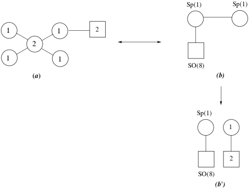
Refer to caption
Figure 19: Doubly Framed D^4subscript^𝐷4\hat{D}_{4} quiver (a)𝑎(a), its Hanany-Witten mirror (b)𝑏(b), and its “good” mirror (b)superscript𝑏(b^{\prime}). The Higgs branches of (a)𝑎(a), (b)𝑏(b) and (b)superscript𝑏(b^{\prime}) are as follows. (a)𝑎(a): the moduli space of 111 SU(2)𝑆𝑈2SU(2) instanton on 2/D^4superscript2subscript^𝐷4\mathbb{C}^{2}/\hat{D}_{4}. (b)𝑏(b): the moduli space of 111 SO(8)𝑆𝑂8SO(8) instanton on 2/2superscript2subscript2\mathbb{C}^{2}/\mathbb{Z}_{2}; see Dey:2013fea . (b)superscript𝑏(b^{\prime}): the reduced instanton moduli space of 111 SO(8)𝑆𝑂8SO(8) instanton on 2superscript2\mathbb{C}^{2} times 2/2superscript2subscript2\mathbb{C}^{2}/\mathbb{Z}_{2}. The factorisation of the Higgs branch of quiver (b)superscript𝑏(b^{\prime}) is discussed in Dey:2013fea .

We cannot be completely satisfied with the (b)𝑏(b) picture in Fig. 19 since the quiver is “bad” on the unframed Sp(1)𝑆𝑝1Sp(1) node. Inability to find a “good” quiver by formally applying the S-duality is not an uncommon phenomenon while working with quivers involving Sp𝑆𝑝Sp and SO𝑆𝑂SO gauge groups Gaiotto:2008ak . Therefore we expect to be able to find another “good” quiver theory which flows in the infrared to the same SCFT as theory (b)𝑏(b) flows to. We will show in this section that this is the quiver (b)superscript𝑏(b^{\prime}) in Fig. 19 from a straightforward application of Abelian gauging using sphere partition functions.

Refer to caption
Refer to caption
Refer to caption
Refer to caption
Figure 20: Mirror linear quivers (top row) and the new mirror pair after the gauging trick (bottom row).

Partition function approach

Consider the partition functions for the linear quivers shown in the top row of Fig. 20. They take the following form

𝒵A(ma;tα)=α=12dsαd2s02!α=12e2πisαηαi=12e2πis0iη0sinh2π(s01s02)i=12coshπ(s1s0i)a=12coshπ(s0i+ma)coshπ(s2s0i)×1a=12coshπ(s2+m2+a)𝒵B(Mα;t~a)=α=12dsαd2s02!α=12e2πisαη~αi=12e2πis0iη~0sinh2π(s01s02)i=12coshπ(s0is1)a=13coshπ(s0i+Ma)coshπ(s1s2)×1coshπ(s2+M4)subscript𝒵𝐴subscript𝑚𝑎subscript𝑡𝛼subscriptsuperscriptproduct2𝛼1𝑑subscript𝑠𝛼superscript𝑑2subscript𝑠02subscriptsuperscriptproduct2𝛼1superscript𝑒2𝜋𝑖subscript𝑠𝛼subscript𝜂𝛼subscriptsuperscriptproduct2𝑖1superscript𝑒2𝜋𝑖subscriptsuperscript𝑠𝑖0subscript𝜂0superscript2𝜋subscriptsuperscript𝑠10subscriptsuperscript𝑠20subscriptsuperscriptproduct2𝑖1𝜋subscript𝑠1subscriptsuperscript𝑠𝑖0subscriptsuperscriptproduct2𝑎1𝜋subscriptsuperscript𝑠𝑖0subscript𝑚𝑎𝜋subscript𝑠2subscriptsuperscript𝑠𝑖01subscriptsuperscriptproduct2𝑎1𝜋subscript𝑠2subscript𝑚2𝑎subscript𝒵𝐵subscript𝑀𝛼subscript~𝑡𝑎subscriptsuperscriptproduct2𝛼1𝑑subscript𝑠𝛼superscript𝑑2subscript𝑠02subscriptsuperscriptproduct2𝛼1superscript𝑒2𝜋𝑖subscript𝑠𝛼subscript~𝜂𝛼subscriptsuperscriptproduct2𝑖1superscript𝑒2𝜋𝑖subscriptsuperscript𝑠𝑖0subscript~𝜂0superscript2𝜋subscriptsuperscript𝑠10subscriptsuperscript𝑠20subscriptsuperscriptproduct2𝑖1𝜋subscriptsuperscript𝑠𝑖0subscript𝑠1subscriptsuperscriptproduct3𝑎1𝜋subscriptsuperscript𝑠𝑖0subscript𝑀𝑎𝜋subscript𝑠1subscript𝑠21𝜋subscript𝑠2subscript𝑀4\begin{split}{\cal Z}_{A}(m_{a};{t}_{\alpha})=&\int\prod^{2}_{\alpha=1}ds_{\alpha}\frac{d^{2}s_{0}}{2!}\frac{\prod^{2}_{\alpha=1}e^{2\pi is_{\alpha}\eta_{\alpha}}\prod^{2}_{i=1}e^{2\pi is^{i}_{0}\eta_{0}}\sinh^{2}{\pi(s^{1}_{0}-s^{2}_{0})}}{\prod^{2}_{i=1}\cosh{\pi(s_{1}-s^{i}_{0})}\prod^{2}_{a=1}\cosh{\pi(s^{i}_{0}+m_{a})}\cosh{\pi(s_{2}-s^{i}_{0})}}\\ &\times\frac{1}{\prod^{2}_{a=1}\cosh{\pi(s_{2}+m_{2+a})}}\\ {\cal Z}_{B}(M_{\alpha};\widetilde{t}_{a})=&\int\prod^{2}_{\alpha=1}ds_{\alpha}\frac{d^{2}s_{0}}{2!}\frac{\prod^{2}_{\alpha=1}e^{2\pi is_{\alpha}\widetilde{\eta}_{\alpha}}\prod^{2}_{i=1}e^{2\pi is^{i}_{0}\widetilde{\eta}_{0}}\sinh^{2}{\pi(s^{1}_{0}-s^{2}_{0})}}{\prod^{2}_{i=1}\cosh{\pi(s^{i}_{0}-s_{1})}\prod^{3}_{a=1}\cosh{\pi(s^{i}_{0}+M_{a})}\cosh{\pi(s_{1}-s_{2})}}\\ &\times\frac{1}{\cosh{\pi(s_{2}+M_{4})}}\end{split} (90)

where a=1,2,3,4;α=1,2,,4formulae-sequence𝑎1234𝛼124a=1,2,3,4;\;\alpha=1,2,\ldots,4. In the A-model, the FI parameters are defined as η1=t1t2,η0=t2t3,η2=t3t4formulae-sequencesubscript𝜂1subscript𝑡1subscript𝑡2formulae-sequencesubscript𝜂0subscript𝑡2subscript𝑡3subscript𝜂2subscript𝑡3subscript𝑡4\eta_{1}=t_{1}-t_{2},\eta_{0}=t_{2}-t_{3},\eta_{2}=t_{3}-t_{4}, while for the B-model, these are η~0=t~1t~2,η~1=t~2t~3,η~2=t~3t~4formulae-sequencesubscript~𝜂0subscript~𝑡1subscript~𝑡2formulae-sequencesubscript~𝜂1subscript~𝑡2subscript~𝑡3subscript~𝜂2subscript~𝑡3subscript~𝑡4\widetilde{\eta}_{0}=\widetilde{t}_{1}-\widetilde{t}_{2},\widetilde{\eta}_{1}=\widetilde{t}_{2}-\widetilde{t}_{3},\widetilde{\eta}_{2}=\widetilde{t}_{3}-\widetilde{t}_{4}. Mirror Symmetry implies that 𝒵A(ma;tα)=𝒵B(Mα;t~a)subscript𝒵𝐴subscript𝑚𝑎subscript𝑡𝛼subscript𝒵𝐵subscript𝑀𝛼subscript~𝑡𝑎{\cal Z}_{A}(m_{a};{t}_{\alpha})={\cal Z}_{B}(M_{\alpha};\widetilde{t}_{a}) up to some overall phase provided the parameters are related as follows:

Mα=tαt~a=ma.subscript𝑀𝛼subscript𝑡𝛼subscript~𝑡𝑎subscript𝑚𝑎\begin{split}&M_{\alpha}={t}_{\alpha}\\ &\widetilde{t}_{a}=m_{a}\,.\end{split} (91)

Now we gauge the left U(2)𝑈2U(2) flavor symmetry in the top left quiver in Fig. 20 as a U(1)×U(1)𝑈1𝑈1U(1)\times U(1), which gives a D^4subscript^𝐷4\hat{D}_{4} quiver with two hypers on a single boundary node (lower left quiver in Fig. 20). The partition function of this theory is

𝒵~A(ζ1,ζ2,m3,m4;tα)=𝑑m1𝑑m2e2πim1ζ1e2πim2ζ2ZA(ma;tα)=𝑑m1𝑑m2e2πim1ζ1e2πim2ζ2ZB(tα;ma),subscript~𝒵𝐴subscript𝜁1subscript𝜁2subscript𝑚3subscript𝑚4subscript𝑡𝛼differential-dsubscript𝑚1differential-dsubscript𝑚2superscript𝑒2𝜋𝑖subscript𝑚1subscript𝜁1superscript𝑒2𝜋𝑖subscript𝑚2subscript𝜁2subscript𝑍𝐴subscript𝑚𝑎subscript𝑡𝛼differential-dsubscript𝑚1differential-dsubscript𝑚2superscript𝑒2𝜋𝑖subscript𝑚1subscript𝜁1superscript𝑒2𝜋𝑖subscript𝑚2subscript𝜁2subscript𝑍𝐵subscript𝑡𝛼subscript𝑚𝑎\begin{split}\widetilde{{\cal Z}}_{A}(\zeta_{1},\zeta_{2},m_{3},m_{4};{t}_{\alpha})=&\int dm_{1}dm_{2}e^{2\pi im_{1}\zeta_{1}}e^{2\pi im_{2}\zeta_{2}}Z_{A}(m_{a};{t}_{\alpha})\\ =&\int dm_{1}dm_{2}e^{2\pi im_{1}\zeta_{1}}e^{2\pi im_{2}\zeta_{2}}Z_{B}({t}_{\alpha};m_{a})\,,\end{split} (92)

where the second equality follows from the mirror symmetry of the linear quivers. From the second equality, completing the integration over m1subscript𝑚1m_{1} and m2subscript𝑚2m_{2} we have

𝒵~A(ζ1,ζ2,m3,m4;tα)=𝑑s2𝑑s1d2s02!δ(s01+s02+ζ1)δ(s01s02+s1+ζ2)sinh2π(s01s02)iα=13coshπ(s0i+tα)×e2πim3s1icoshπ(s0is1)×e2πi(m3m4)s2coshπ(s1s2)coshπ(s2+t4)subscript~𝒵𝐴subscript𝜁1subscript𝜁2subscript𝑚3subscript𝑚4subscript𝑡𝛼differential-dsubscript𝑠2differential-dsubscript𝑠1superscript𝑑2subscript𝑠02𝛿subscriptsuperscript𝑠10subscriptsuperscript𝑠20subscript𝜁1𝛿subscriptsuperscript𝑠10subscriptsuperscript𝑠20subscript𝑠1subscript𝜁2superscript2𝜋subscriptsuperscript𝑠10subscriptsuperscript𝑠20subscriptproduct𝑖subscriptsuperscriptproduct3𝛼1𝜋subscriptsuperscript𝑠𝑖0subscript𝑡𝛼superscript𝑒2𝜋𝑖subscript𝑚3subscript𝑠1subscriptproduct𝑖𝜋subscriptsuperscript𝑠𝑖0subscript𝑠1superscript𝑒2𝜋𝑖subscript𝑚3subscript𝑚4subscript𝑠2𝜋subscript𝑠1subscript𝑠2𝜋subscript𝑠2subscript𝑡4\begin{split}\widetilde{{\cal Z}}_{A}(\zeta_{1},\zeta_{2},m_{3},m_{4};{t}_{\alpha})=&\int ds_{2}ds_{1}\frac{d^{2}s_{0}}{2!}\frac{\delta(s^{1}_{0}+s^{2}_{0}+\zeta_{1})\delta(-s^{1}_{0}-s^{2}_{0}+s_{1}+\zeta_{2})\sinh^{2}{\pi(s^{1}_{0}-s^{2}_{0})}}{\prod_{i}\prod^{3}_{\alpha=1}\cosh{\pi(s^{i}_{0}+t_{\alpha})}}\\ &\times\frac{e^{-2\pi im_{3}s_{1}}}{\prod_{i}\cosh{\pi(s^{i}_{0}-s_{1})}}\times\frac{e^{2\pi i(m_{3}-m_{4})s_{2}}}{\cosh{\pi(s_{1}-s_{2})}\cosh{\pi(s_{2}+t_{4})}}\end{split} (93)

Finally, integrating over s1subscript𝑠1s_{1} using the delta function and shifting the remaining integration variables appropriately, we have

𝒵~A(ζ1,ζ2,m3,m4;tα)=e2πim3(ζ1+ζ2)d2s02!δ(s01+s02)sinh2π(s01s02)iα=13coshπ(s0i+tαζ12)icoshπ(s0i+ζ1+ζ2)×ds2e2πi(m3m4)s2coshπ(s2t4)coshπ(s2+ζ1+ζ2)=𝒵~B(Mi,Ma;t3~,t~4)subscript~𝒵𝐴subscript𝜁1subscript𝜁2subscript𝑚3subscript𝑚4subscript𝑡𝛼superscript𝑒2𝜋𝑖subscript𝑚3subscript𝜁1subscript𝜁2superscript𝑑2subscript𝑠02𝛿subscriptsuperscript𝑠10subscriptsuperscript𝑠20superscript2𝜋subscriptsuperscript𝑠10subscriptsuperscript𝑠20subscriptproduct𝑖subscriptsuperscriptproduct3𝛼1𝜋subscriptsuperscript𝑠𝑖0subscript𝑡𝛼subscript𝜁12subscriptproduct𝑖𝜋subscriptsuperscript𝑠𝑖0subscript𝜁1subscript𝜁2𝑑subscript𝑠2superscript𝑒2𝜋𝑖subscript𝑚3subscript𝑚4subscript𝑠2𝜋subscript𝑠2subscript𝑡4𝜋subscript𝑠2subscript𝜁1subscript𝜁2subscript~𝒵𝐵subscript𝑀𝑖subscript𝑀𝑎~subscript𝑡3subscript~𝑡4\begin{split}\widetilde{{\cal Z}}_{A}(\zeta_{1},\zeta_{2},m_{3},m_{4};{t}_{\alpha})=&e^{2\pi im_{3}(\zeta_{1}+\zeta_{2})}\int\frac{d^{2}s_{0}}{2!}\frac{\delta(s^{1}_{0}+s^{2}_{0})\sinh^{2}{\pi(s^{1}_{0}-s^{2}_{0})}}{\prod_{i}\prod^{3}_{\alpha=1}\cosh{\pi(s^{i}_{0}+t_{\alpha}-\frac{\zeta_{1}}{2})}\prod_{i}\cosh{\pi(s^{i}_{0}+\zeta_{1}+\zeta_{2})}}\\ &\times\int ds_{2}\frac{e^{2\pi i(m_{3}-m_{4})s_{2}}}{\cosh{\pi(s_{2}-t_{4})}\cosh{\pi(s_{2}+\zeta_{1}+\zeta_{2})}}\\ =&\widetilde{{\cal Z}}_{B}(M_{i},M_{a};\widetilde{t_{3}},\widetilde{t}_{4})\end{split} (94)

The dual theory therefore splits into two parts – an Sp(1)𝑆𝑝1Sp(1) gauge theory with 4 flavors whose partition function is given by the first line (masses labeled as Misubscript𝑀𝑖M_{i} with i=1,2,3,4𝑖1234i=1,2,3,4) and a U(1)𝑈1U(1) gauge theory with 2 flavors whose partition function is given by the second line (masses labeled as Masubscript𝑀𝑎M_{a} with a=5,6𝑎56a=5,6).

The mirror map for this mirror pair can then be directly read off from the above partition function.

Ma=ta+ζ12,a=1,2,3M4=ζ12+ζ2t~j=mj,j=3,4M5=t4M6=ζ1+ζ2.\begin{split}&M_{a}=t_{a}+\frac{\zeta_{1}}{2}\,,\quad\;a=1,2,3\\ &M_{4}=\frac{\zeta_{1}}{2}+\zeta_{2}\\ &\widetilde{t}_{j}=m_{j}\,,\quad\;\;j=3,4\\ &M_{5}=t_{4}\\ &M_{6}=\zeta_{1}+\zeta_{2}\,.\end{split} (95)

Note that the number of parameters exactly match on both sides. For the A-model, we have five independent FI parameters – {t1,t2,t3,t4}subscript𝑡1subscript𝑡2subscript𝑡3subscript𝑡4\{t_{1},t_{2},t_{3},t_{4}\} with one constraint and {ζ1,ζ2}subscript𝜁1subscript𝜁2\{\zeta_{1},\zeta_{2}\}. This is matched by the 5 independent mass parameters for the B-model – 6 mass parameters with the following constraint

M1+M2+M3+M5=3(M6M4).subscript𝑀1subscript𝑀2subscript𝑀3subscript𝑀53subscript𝑀6subscript𝑀4M_{1}+M_{2}+M_{3}+M_{5}=3(M_{6}-M_{4}). (96)

Similarly, two mass parameters on the A-model side coincides with the two t~asubscript~𝑡𝑎\widetilde{t}_{a} parameters on the B-model side.

In general, in order to obtain a mirror pair in this class for N>4𝑁4N>4 by gauging, we start from the following linear quivers:
A-model: (1,0)(2,1)1(2,0)2(2,0)N4(2,1)N3(1,2)N210subscript211subscript202subscript20𝑁4subscript21𝑁3subscript12𝑁2(1,0)(2,1)_{1}(2,0)_{2}\ldots(2,0)_{N-4}(2,1)_{N-3}(1,2)_{N-2} and
B-model: (2,N1)(1,0)(1,1)2𝑁11011(2,N-1)(1,0)(1,1).

One needs to gauge the U(1)𝑈1U(1) flavor symmetries of the nodes (2,1)1subscript211(2,1)_{1} and (2,1)N3subscript21𝑁3(2,1)_{N-3} to obtain the appropriately framed D^Nsubscript^𝐷𝑁\hat{D}_{N} quiver. Proceeding as before, the mirror is found to consist of a Sp(1)𝑆𝑝1Sp(1) gauge theory with N𝑁N fundamental hypers and a decoupled U(1)𝑈1U(1) gauge theory with two hypers. The mirror map in this case is an obvious generalization of the D^4subscript^𝐷4\hat{D}_{4} case.

Ma=ta+ζ12(a=1,2,,N1)MN=ζ12+ζ2t~j=mj(j=3,4)MN+1=t4MN+2=ζ1+ζ2.subscript𝑀𝑎subscript𝑡𝑎subscript𝜁12𝑎12𝑁1subscript𝑀𝑁subscript𝜁12subscript𝜁2subscript~𝑡𝑗subscript𝑚𝑗𝑗34subscript𝑀𝑁1subscript𝑡4subscript𝑀𝑁2subscript𝜁1subscript𝜁2\begin{split}&M_{a}=t_{a}+\frac{\zeta_{1}}{2}\;(a=1,2,\ldots,N-1)\\ &M_{N}=\frac{\zeta_{1}}{2}+\zeta_{2}\\ &\widetilde{t}_{j}=m_{j}\;(j=3,4)\\ &M_{N+1}=t_{4}\\ &M_{N+2}=\zeta_{1}+\zeta_{2}\,.\end{split} (97)

Checking Mirror Symmetry in Fig. 19 by using Hilbert series

It is instructive to check the result by computing the corresponding Hilbert series and in particular the fact that the (b)superscript𝑏(b^{\prime}) quiver in Fig. 19 is indeed a disjoint union of two quivers. In what follows we compute both Higgs and Coulomb branch series. Note that in the Higgs branch Hilbert series we use

τ=t1/2.𝜏superscript𝑡12\displaystyle\tau=t^{1/2}~{}. (98)

The Higgs branch Hilbert series of diagram (a) in Fig. 19 is given by the gluing technique Benvenuti:2010pq ; Hanany:2011db :

H(a)H(τ,x)subscriptsuperscript𝐻𝐻𝑎𝜏𝑥\displaystyle H^{H}_{(a)}(\tau,x) =(i=14|qi|=1dqi2πiqi)(12i=12|zi|=1dzi2πizi)(z1z2)(z11z21)×\displaystyle=\left(\prod_{i=1}^{4}\oint_{|q_{i}|=1}\frac{\mathrm{d}q_{i}}{2\pi iq_{i}}\right)\left(\frac{1}{2}\prod_{i=1}^{2}\oint_{|z_{i}|=1}\frac{\mathrm{d}z_{i}}{2\pi iz_{i}}\right)(z_{1}-z_{2})(z_{1}^{-1}-z_{2}^{-1})\times
χ(1)[2](τ;q1;x)i=14χ(2)(1)i(τ;qi;𝒛),subscript𝜒1delimited-[]2𝜏subscript𝑞1𝑥superscriptsubscriptproduct𝑖14subscript𝜒2subscript1𝑖𝜏subscript𝑞𝑖𝒛\displaystyle\qquad\chi_{(1)-[2]}(\tau;q_{1};x)\prod_{i=1}^{4}\chi_{(2)-(1)_{i}}(\tau;q_{i};\bm{z})~{}, (99)

where q1,q4subscript𝑞1subscript𝑞4q_{1},\ldots q_{4} denote the gauge fugacities of the four U(1)𝑈1U(1) gauge groups, z1,z2subscript𝑧1subscript𝑧2z_{1},z_{2} denote the gauge fugacities of the U(2)𝑈2U(2) gauge group, (x,y)𝑥𝑦(x,y) denotes the fugacities of the U(2)=U(1)×SU(2)𝑈2𝑈1𝑆𝑈2U(2)=U(1)\times SU(2) flavour node, and the contributions from the hypermultiplets are

χ(1)[2](τ;q1;x,y)subscript𝜒1delimited-[]2𝜏subscript𝑞1𝑥𝑦\displaystyle\chi_{(1)-[2]}(\tau;q_{1};x,y) =PE[τ(q1x1+q11x)(y+y1)],absentPEdelimited-[]𝜏subscript𝑞1superscript𝑥1superscriptsubscript𝑞11𝑥𝑦superscript𝑦1\displaystyle=\mathop{\rm PE}\left[\tau(q_{1}x^{-1}+q_{1}^{-1}x)(y+y^{-1})\right]~{},
χ(2)(1)i(τ;qi;𝒛)subscript𝜒2subscript1𝑖𝜏subscript𝑞𝑖𝒛\displaystyle\chi_{(2)-(1)_{i}}(\tau;q_{i};\bm{z}) =PE[τ(z1+z2)qi1+τ(z11+z21)qi],absentPEdelimited-[]𝜏subscript𝑧1subscript𝑧2superscriptsubscript𝑞𝑖1𝜏superscriptsubscript𝑧11superscriptsubscript𝑧21subscript𝑞𝑖\displaystyle=\mathop{\rm PE}\left[\tau(z_{1}+z_{2})q_{i}^{-1}+\tau(z_{1}^{-1}+z_{2}^{-1})q_{i}\right]~{}, (100)

with the plethystic exponential PEPE\mathop{\rm PE} of a multivariate function f(a1,a2,,an)𝑓subscript𝑎1subscript𝑎2subscript𝑎𝑛f(a_{1},a_{2},\ldots,a_{n}), with f(0,0,,0)=0𝑓0000f(0,0,\ldots,0)=0, defined as

PE[f(a1,a2,,an)]=exp(k=11kf(a1k,a2k,,ank)).PEdelimited-[]𝑓subscript𝑎1subscript𝑎2subscript𝑎𝑛superscriptsubscript𝑘11𝑘𝑓superscriptsubscript𝑎1𝑘superscriptsubscript𝑎2𝑘superscriptsubscript𝑎𝑛𝑘\displaystyle\mathop{\rm PE}[f(a_{1},a_{2},\ldots,a_{n})]=\exp\left(\sum_{k=1}^{\infty}\frac{1}{k}f(a_{1}^{k},a_{2}^{k},\ldots,a_{n}^{k})\right)~{}. (101)

As a result of the integrations, we find that

H(a)H(τ,y)subscriptsuperscript𝐻𝐻𝑎𝜏𝑦\displaystyle H^{H}_{(a)}(\tau,y) =1τ12(1τ4)2(1τ6)m=0[2m]yτ2mabsent1superscript𝜏12superscript1superscript𝜏421superscript𝜏6superscriptsubscript𝑚0subscriptdelimited-[]2𝑚𝑦superscript𝜏2𝑚\displaystyle=\frac{1-\tau^{12}}{(1-\tau^{4})^{2}(1-\tau^{6})}\sum_{m=0}^{\infty}[2m]_{y}\tau^{2m} (102)

This is indeed the Hilbert series of (2/D^4)×(2/2)superscript2subscript^𝐷4superscript2subscript2(\mathbb{C}^{2}/\hat{D}_{4})\times(\mathbb{C}^{2}/\mathbb{Z}_{2}) Benvenuti:2006qr ; this is in agreement with the Coulomb branch of diagram (bsuperscript𝑏b^{\prime}) of Fig. 19.

The Coulomb branch Hilbert series of diagram (a) in Fig. 19 is given by

H(a)C(t,𝒂,𝒃)subscriptsuperscript𝐻𝐶𝑎𝑡𝒂𝒃\displaystyle H^{C}_{(a)}(t,\bm{a},\bm{b}) =m1=m2=m1n1=n4=PU(2)(t,m1,m2)PU(1)(t)4i=12aimij=14bjnjabsentsuperscriptsubscriptsubscript𝑚1superscriptsubscriptsubscript𝑚2subscript𝑚1superscriptsubscriptsubscript𝑛1superscriptsubscriptsubscript𝑛4subscript𝑃𝑈2𝑡subscript𝑚1subscript𝑚2subscript𝑃𝑈1superscript𝑡4superscriptsubscriptproduct𝑖12superscriptsubscript𝑎𝑖subscript𝑚𝑖superscriptsubscriptproduct𝑗14superscriptsubscript𝑏𝑗subscript𝑛𝑗\displaystyle=\sum_{m_{1}=-\infty}^{\infty}\sum_{m_{2}=-\infty}^{m_{1}}\sum_{n_{1}=-\infty}^{\infty}\cdots\sum_{n_{4}=-\infty}^{\infty}P_{U(2)}(t,m_{1},m_{2})P_{U(1)}(t)^{4}\prod_{i=1}^{2}a_{i}^{m_{i}}\prod_{j=1}^{4}b_{j}^{n_{j}}

where m1,m2subscript𝑚1subscript𝑚2m_{1},m_{2} are the monopole charges associated with the U(2)𝑈2U(2) gauge group, and n1,,n4subscript𝑛1subscript𝑛4n_{1},\ldots,n_{4} are the monopole charges associated with each U(1)𝑈1U(1) gauge group. Here Δ(𝒎,𝒏)Δ𝒎𝒏\Delta(\bm{m},\bm{n}) is the dimension of the monopole operators:

Δ(m1,m2,n1,,n4)=12(2|n1|+i=12j=14|minj|)|m1m2|,Δsubscript𝑚1subscript𝑚2subscript𝑛1subscript𝑛4122subscript𝑛1superscriptsubscript𝑖12superscriptsubscript𝑗14subscript𝑚𝑖subscript𝑛𝑗subscript𝑚1subscript𝑚2\displaystyle\Delta(m_{1},m_{2},n_{1},\ldots,n_{4})=\frac{1}{2}\left(2|n_{1}|+\sum_{i=1}^{2}\sum_{j=1}^{4}|m_{i}-n_{j}|\right)-|m_{1}-m_{2}|~{}, (104)

and the functions PU(2)(t,𝒎)subscript𝑃𝑈2𝑡𝒎P_{U(2)}(t,\bm{m}) and PU(1)(t)subscript𝑃𝑈1𝑡P_{U(1)}(t) are defined as

PU(1)(t)subscript𝑃𝑈1𝑡\displaystyle P_{U(1)}(t) =11t,absent11𝑡\displaystyle=\frac{1}{1-t}~{},
PU(2)(t,𝒎)subscript𝑃𝑈2𝑡𝒎\displaystyle P_{U(2)}(t,\bm{m}) ={1(1t)2,m1m21(1t)(1t2),m1=m2.absentcases1superscript1𝑡2subscript𝑚1subscript𝑚211𝑡1superscript𝑡2subscript𝑚1subscript𝑚2\displaystyle=\begin{cases}\frac{1}{(1-t)^{2}}~{},&\qquad m_{1}\neq m_{2}\\ \frac{1}{(1-t)(1-t^{2})}~{},&\qquad m_{1}=m_{2}~{}.\end{cases} (105)

Setting ai=bj=1subscript𝑎𝑖subscript𝑏𝑗1a_{i}=b_{j}=1 for all i,j𝑖𝑗i,j, we obtain

H(a)C(t,{ai=1},{bj=1})subscriptsuperscript𝐻𝐶𝑎𝑡subscript𝑎𝑖1subscript𝑏𝑗1\displaystyle H^{C}_{(a)}(t,\{a_{i}=1\},\{b_{j}=1\}) =1+19t+83t2+130t3+83t4+19t5+t6(1t)12absent119𝑡83superscript𝑡2130superscript𝑡383superscript𝑡419superscript𝑡5superscript𝑡6superscript1𝑡12\displaystyle=\frac{1+19t+83t^{2}+130t^{3}+83t^{4}+19t^{5}+t^{6}}{(1-t)^{12}}
=(1+t)2(1+17t+48t2+17t3+t4)(1t)12.absentsuperscript1𝑡2117𝑡48superscript𝑡217superscript𝑡3superscript𝑡4superscript1𝑡12\displaystyle=\frac{(1+t)^{2}\left(1+17t+48t^{2}+17t^{3}+t^{4}\right)}{(1-t)^{12}}~{}. (106)

The order of the pole at t=1𝑡1t=1 is 12; this is equal to the complex dimension of the Coulomb branch as expected.

Then we investigate the Higgs branch of diagram (b) in Fig. 19. The space of F-term solutions (also known as the F-flat space) of quiver in diagram (b) of Fig. 19 can be decomposed into many branches. The branch that leads to the Higgs branch after imposing the D𝐷D-term constraints is the 18 complex dimensional branch. The Hilbert series of this branch can be obtained using Macaulay2 M2 . The closed form is, however, too lengthy to be reported here; let us present a few terms in the series expansion:

(τ;z1,z2;x,𝒚)=1+([1,0,0,0]𝒚[1]z1+[1]x[1]z1[1]z2)τ+,superscript𝜏subscript𝑧1subscript𝑧2𝑥𝒚1subscript1000𝒚subscriptdelimited-[]1subscript𝑧1subscriptdelimited-[]1𝑥subscriptdelimited-[]1subscript𝑧1subscriptdelimited-[]1subscript𝑧2𝜏\displaystyle\mathcal{F}^{\flat}(\tau;z_{1},z_{2};x,\bm{y})=1+([1,0,0,0]_{\bm{y}}[1]_{z_{1}}+[1]_{x}[1]_{z_{1}}[1]_{z_{2}})\tau+\ldots~{}, (107)

where z1,z2subscript𝑧1subscript𝑧2z_{1},z_{2} are gauge fugacities for each Sp(1)𝑆𝑝1Sp(1) gauge group, x𝑥x is the global SU(2)𝑆𝑈2SU(2) fugacity that transform the chiral fields in hypermultiplet in Sp(1)×Sp(1)𝑆𝑝1𝑆𝑝1Sp(1)\times Sp(1), and y1,,y4subscript𝑦1subscript𝑦4y_{1},\ldots,y_{4} are the fugacities of the SO(8)𝑆𝑂8SO(8) flavour symmetry. The corresponding unrefined Hilbert series is

(τ;z1=z2=1;x=1,{yi=1})=(1+τ)3(1+3τ)(1τ)18.\displaystyle\mathcal{F}^{\flat}(\tau;z_{1}=z_{2}=1;x=1,\{y_{i}=1\})=\frac{(1+\tau)^{3}(1+3\tau)}{(1-\tau)^{18}}~{}. (108)

After implementing gauge invariance, the Higgs branch Hilbert series is given by

H(b)H(τ,x,𝒚)subscriptsuperscript𝐻𝐻𝑏𝜏𝑥𝒚\displaystyle H^{H}_{(b)}(\tau,x,\bm{y}) =|z1|=1dz12πiz11z12z1|z2|=1dz22πiz21z22z2(τ;z1,z2;x,𝒚)absentsubscriptcontour-integralsubscript𝑧11dsubscript𝑧12𝜋𝑖subscript𝑧11superscriptsubscript𝑧12subscript𝑧1subscriptcontour-integralsubscript𝑧21dsubscript𝑧22𝜋𝑖subscript𝑧21superscriptsubscript𝑧22subscript𝑧2superscript𝜏subscript𝑧1subscript𝑧2𝑥𝒚\displaystyle=\oint_{|z_{1}|=1}\frac{\mathrm{d}z_{1}}{2\pi iz_{1}}\frac{1-z_{1}^{2}}{z_{1}}\oint_{|z_{2}|=1}\frac{\mathrm{d}z_{2}}{2\pi iz_{2}}\;\frac{1-z_{2}^{2}}{z_{2}}\mathcal{F}^{\flat}(\tau;z_{1},z_{2};x,\bm{y})
=m=0[2m]xτ2m×n=0[0,n,0,0]𝒚τ2n.absentsuperscriptsubscript𝑚0subscriptdelimited-[]2𝑚𝑥superscript𝜏2𝑚superscriptsubscript𝑛0subscript0𝑛00𝒚superscript𝜏2𝑛\displaystyle=\sum_{m=0}^{\infty}[2m]_{x}\tau^{2m}\times\sum_{n=0}^{\infty}[0,n,0,0]_{\bm{y}}\tau^{2n}~{}. (109)

This Hilbert series indicates that the Higgs branch of the diagram (b) of Fig. 19 is indeed

2/2×SU(2) w/ 4 flv,superscript2subscript2subscriptSU(2) w/ 4 flv\displaystyle\mathbb{C}^{2}/\mathbb{Z}_{2}\times{\cal H}_{\text{$SU(2)$ w/ 4 flv}}~{}, (110)

where SU(2) w/ 4 flvsubscriptSU(2) w/ 4 flv{\cal H}_{\text{$SU(2)$ w/ 4 flv}} is the Higgs branch of SU(2)𝑆𝑈2SU(2) with 444 flavours. Therefore, this agrees with the Higgs branch of the (b)superscript𝑏(b^{\prime}) quiver in Fig. 20.

Setting x=1𝑥1x=1 and yi=1subscript𝑦𝑖1y_{i}=1, we obtain the unrefined Higgs branch Hilbert series

H(b)H(τ,x=1,{yi=1})\displaystyle H^{H}_{(b)}(\tau,x=1,\{y_{i}=1\}) =1τ4(1τ2)3×(1+τ2)(1+17τ2+48τ4+17τ6+τ8)(1τ2)10absent1superscript𝜏4superscript1superscript𝜏231superscript𝜏2117superscript𝜏248superscript𝜏417superscript𝜏6superscript𝜏8superscript1superscript𝜏210\displaystyle=\frac{1-\tau^{4}}{(1-\tau^{2})^{3}}\times\frac{\left(1+\tau^{2}\right)\left(1+17\tau^{2}+48\tau^{4}+17\tau^{6}+\tau^{8}\right)}{\left(1-\tau^{2}\right)^{10}}
=(1+τ2)2(1+17τ2+48τ4+17τ6+τ8)(1τ2)12absentsuperscript1superscript𝜏22117superscript𝜏248superscript𝜏417superscript𝜏6superscript𝜏8superscript1superscript𝜏212\displaystyle=\frac{\left(1+\tau^{2}\right)^{2}\left(1+17\tau^{2}+48\tau^{4}+17\tau^{6}+\tau^{8}\right)}{\left(1-\tau^{2}\right)^{12}}
=H(a)C(τ2,{ai=1},{bj=1}).absentsubscriptsuperscript𝐻𝐶𝑎superscript𝜏2subscript𝑎𝑖1subscript𝑏𝑗1\displaystyle=H^{C}_{(a)}(\tau^{2},\{a_{i}=1\},\{b_{j}=1\})~{}. (111)

Note that this is in agreement with (4.4), thereby providing a very non-trivial check of the proposed mirror symmetry.

General results

One can easily generalize the above computation to determine the mirror of a D^Nsubscript^𝐷𝑁\hat{D}_{N} quiver with M>2𝑀2M>2 fundamental hypers on one of the external nodes, as shown in Fig. 21.
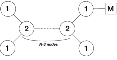
Refer to caption
Refer to caption
Figure 21: D^Nsubscript^𝐷𝑁\hat{D}_{N} quiver with M𝑀M hypermultiplets on the edge node and its mirror. The Higgs branch of the left quiver is the moduli space of 111 SU(M)𝑆𝑈𝑀SU(M) instanton on 2/D^Nsuperscript2subscript^𝐷𝑁\mathbb{C}^{2}/\hat{D}_{N} and that of the right quiver is the moduli space of 111 SO(2N)𝑆𝑂2𝑁SO(2N) instanton on 2/Msuperscript2subscript𝑀\mathbb{C}^{2}/\mathbb{Z}_{M}. The latter factorises into 2/Msuperscript2subscript𝑀\mathbb{C}^{2}/\mathbb{Z}_{M} times the reduced instanton moduli space of 111 SO(2N)𝑆𝑂2𝑁SO(2N) instanton on 2superscript2\mathbb{C}^{2}; see Dey:2013fea .

The starting point is the mirror pair consisting of the following linear quivers:
A-model: (1,0)(2,1)1(2,0)2(2,0)N4(2,1)N3(1,M)N210subscript211subscript202subscript20𝑁4subscript21𝑁3subscript1𝑀𝑁2(1,0)(2,1)_{1}(2,0)_{2}\ldots(2,0)_{N-4}(2,1)_{N-3}(1,M)_{N-2} and
B-model: (2,N1)(1,0)1(1,0)M1(1,1)M2𝑁1subscript101subscript10𝑀1subscript11𝑀(2,N-1)(1,0)_{1}\ldots(1,0)_{M-1}(1,1)_{M}.

Again gauging the U(1)𝑈1U(1) flavor symmetries of the nodes (2,1)1subscript211(2,1)_{1} and (2,1)N3subscript21𝑁3(2,1)_{N-3} to obtain the appropriately framed D^Nsubscript^𝐷𝑁\hat{D}_{N} quiver, we find that the dual theory consists of a Sp(1)𝑆𝑝1Sp(1) gauge theory with N𝑁N fundamental hypers and a decoupled quiver gauge theory (1,1)1(1,0)2(1,0)M2(1,1)M1subscript111subscript102subscript10𝑀2subscript11𝑀1(1,1)_{1}(1,0)_{2}\ldots(1,0)_{M-2}(1,1)_{M-1}. The mirror map is an obvious generalization of the one obtained for M=2𝑀2M=2.

4.4.3 Framing at two different nodes of D^4subscript^𝐷4\hat{D}_{4} quiver

As a final example of this section let us consider a situation presented in Fig. 22 for D^4subscript^𝐷4\hat{D}_{4} quiver, when two of the boundary nodes of the tail are framed.
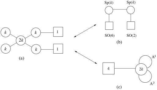
Refer to caption
Figure 22: Two possible mirrors for D^4subscript^𝐷4\hat{D}_{4} quiver (a).

Clearly, the D^4subscript^𝐷4\hat{D}_{4} quiver shown in Fig. 22 is somewhat special as it has more symmetries than a generic D^Nsubscript^𝐷𝑁\hat{D}_{N} quiver. Below we shall work in detail on two families of doubly framed D^Nsubscript^𝐷𝑁\hat{D}_{N} quivers shown in Fig. 26 and Fig. 24 which coincide for N=4𝑁4N=4 as we have already seen in Fig. 22

Mirror Dual with a Unitary Gauge Group

Consider the mirror theory corresponding to the lower arrow first. The appropriate linear quiver in this case is (1,1)(2,2)(1,1)112211(1,1)(2,2)(1,1) (see Fig. 23). Note that this is a self-mirror.
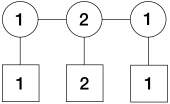
Refer to caption
Figure 23: Linear A3subscript𝐴3A_{3} quiver with labels (1,1)(2,2)(1,1)112211(1,1)(2,2)(1,1).

Its partition functions reads

𝒵A(ma;ta)=α=12dsαd2s02!α=12e2πisαηαi=12e2πis0iη0sinh2π(s01s02)coshπ(s1+m1)i=12coshπ(s1s0i)a=12coshπ(s0i+m1+a)×1i=12coshπ(s2s0i)coshπ(s2+m4).subscript𝒵𝐴subscript𝑚𝑎subscript𝑡𝑎subscriptsuperscriptproduct2𝛼1𝑑subscript𝑠𝛼superscript𝑑2subscript𝑠02subscriptsuperscriptproduct2𝛼1superscript𝑒2𝜋𝑖subscript𝑠𝛼subscript𝜂𝛼subscriptsuperscriptproduct2𝑖1superscript𝑒2𝜋𝑖subscriptsuperscript𝑠𝑖0subscript𝜂0superscript2𝜋subscriptsuperscript𝑠10subscriptsuperscript𝑠20𝜋subscript𝑠1subscript𝑚1subscriptsuperscriptproduct2𝑖1𝜋subscript𝑠1subscriptsuperscript𝑠𝑖0subscriptsuperscriptproduct2𝑎1𝜋subscriptsuperscript𝑠𝑖0subscript𝑚1𝑎1subscriptsuperscriptproduct2𝑖1𝜋subscript𝑠2subscriptsuperscript𝑠𝑖0𝜋subscript𝑠2subscript𝑚4\begin{split}{\cal Z}_{A}(m_{a};{t}_{a})=&\int\prod^{2}_{\alpha=1}ds_{\alpha}\frac{d^{2}s_{0}}{2!}\frac{\prod^{2}_{\alpha=1}e^{2\pi is_{\alpha}\eta_{\alpha}}\prod^{2}_{i=1}e^{2\pi is^{i}_{0}\eta_{0}}\sinh^{2}{\pi(s^{1}_{0}-s^{2}_{0})}}{\cosh{\pi(s_{1}+m_{1})}\prod^{2}_{i=1}\cosh{\pi(s_{1}-s^{i}_{0})}\prod^{2}_{a=1}\cosh{\pi(s^{i}_{0}+m_{1+a})}}\\ &\times\frac{1}{\prod^{2}_{i=1}\cosh{\pi(s_{2}-s^{i}_{0})}\cosh{\pi(s_{2}+m_{4})}}\,.\end{split} (112)

As before, we define η1=t1t2subscript𝜂1subscript𝑡1subscript𝑡2\eta_{1}=t_{1}-t_{2}, η0=t2t3subscript𝜂0subscript𝑡2subscript𝑡3\eta_{0}=t_{2}-t_{3} and η2=t3t4subscript𝜂2subscript𝑡3subscript𝑡4\eta_{2}=t_{3}-t_{4}.
The partition function of the mirror dual, which in this case is the same theory, simply involves the exchange of parameters matasubscript𝑚𝑎subscript𝑡𝑎m_{a}\leftrightarrow t_{a}. Up to some overall phase which we will ignore in this discussion, we have

𝒵B(Ma;t~a)=𝒵A(ta;ma).subscript𝒵𝐵subscript𝑀𝑎subscript~𝑡𝑎subscript𝒵𝐴subscript𝑡𝑎subscript𝑚𝑎{\cal Z}_{B}(M_{a};\widetilde{t}_{a})={\cal Z}_{A}(t_{a};m_{a})\,. (113)

Now we gauge the U(2)𝑈2U(2) flavor symmetry of the A-model as a U(1)×U(1)𝑈1𝑈1U(1)\times U(1), which gives a D^4subscript^𝐷4\hat{D}_{4} quiver with two hypers on a single boundary node. The partition function of this theory is

𝒵~A(m1,ζ2,ζ3,m4;ta)=𝑑m2𝑑m3e2πim2ζ2e2πim3ζ3𝒵A(ma;ta)=𝑑m2𝑑m3e2πim2ζ2e2πim3ζ3𝒵B(ta;ma),subscript~𝒵𝐴subscript𝑚1subscript𝜁2subscript𝜁3subscript𝑚4subscript𝑡𝑎differential-dsubscript𝑚2differential-dsubscript𝑚3superscript𝑒2𝜋𝑖subscript𝑚2subscript𝜁2superscript𝑒2𝜋𝑖subscript𝑚3subscript𝜁3subscript𝒵𝐴subscript𝑚𝑎subscript𝑡𝑎differential-dsubscript𝑚2differential-dsubscript𝑚3superscript𝑒2𝜋𝑖subscript𝑚2subscript𝜁2superscript𝑒2𝜋𝑖subscript𝑚3subscript𝜁3subscript𝒵𝐵subscript𝑡𝑎subscript𝑚𝑎\begin{split}\widetilde{{\cal Z}}_{A}(m_{1},\zeta_{2},\zeta_{3},m_{4};{t}_{a})=&\int dm_{2}dm_{3}e^{2\pi im_{2}\zeta_{2}}e^{2\pi im_{3}\zeta_{3}}{\cal Z}_{A}(m_{a};{t}_{a})\\ =&\int dm_{2}dm_{3}e^{2\pi im_{2}\zeta_{2}}e^{2\pi im_{3}\zeta_{3}}{\cal Z}_{B}({t}_{a};m_{a})\,,\end{split} (114)

where the second equality follows from the mirror symmetry of the linear quivers. From the second equality, completing the integration over m2subscript𝑚2m_{2} and m3subscript𝑚3m_{3} we have

𝒵~A(m1,ζ2,ζ3,m4;ta)=𝑑s2𝑑s1d2s02!δ(s01+s02s1+ζ2)δ(s01+s02s2ζ3)sinh2π(s01s02)iα=23coshπ(s0i+tα)coshπ(s0is1)coshπ(s0is2)×e2πim1s1e2πim4s2coshπ(s1+t1)coshπ(s2+t4).subscript~𝒵𝐴subscript𝑚1subscript𝜁2subscript𝜁3subscript𝑚4subscript𝑡𝑎differential-dsubscript𝑠2differential-dsubscript𝑠1superscript𝑑2subscript𝑠02𝛿subscriptsuperscript𝑠10subscriptsuperscript𝑠20subscript𝑠1subscript𝜁2𝛿subscriptsuperscript𝑠10subscriptsuperscript𝑠20subscript𝑠2subscript𝜁3superscript2𝜋subscriptsuperscript𝑠10subscriptsuperscript𝑠20subscriptproduct𝑖subscriptsuperscriptproduct3𝛼2𝜋subscriptsuperscript𝑠𝑖0subscript𝑡𝛼𝜋subscriptsuperscript𝑠𝑖0subscript𝑠1𝜋subscriptsuperscript𝑠𝑖0subscript𝑠2superscript𝑒2𝜋𝑖subscript𝑚1subscript𝑠1superscript𝑒2𝜋𝑖subscript𝑚4subscript𝑠2𝜋subscript𝑠1subscript𝑡1𝜋subscript𝑠2subscript𝑡4\begin{split}\widetilde{{\cal Z}}_{A}(m_{1},\zeta_{2},\zeta_{3},m_{4};{t}_{a})=&\int ds_{2}ds_{1}\frac{d^{2}s_{0}}{2!}\frac{\delta(s^{1}_{0}+s^{2}_{0}-s_{1}+\zeta_{2})\delta(s^{1}_{0}+s^{2}_{0}-s_{2}-\zeta_{3})\sinh^{2}{\pi(s^{1}_{0}-s^{2}_{0})}}{\prod_{i}\prod^{3}_{\alpha=2}\cosh{\pi(s^{i}_{0}+t_{\alpha})}\cosh{\pi(s^{i}_{0}-s_{1})}\cosh{\pi(s^{i}_{0}-s_{2})}}\\ &\times\frac{e^{2\pi im_{1}s_{1}}e^{-2\pi im_{4}s_{2}}}{\cosh{\pi(s_{1}+t_{1})}\cosh{\pi(s_{2}+t_{4})}}\,.\end{split} (115)

Finally, integrating over s1subscript𝑠1s_{1} and s2subscript𝑠2s_{2} using the delta functions and shifting the remaining integration variables appropriately, we have

𝒵~A(m1,ζ2,ζ3,m4;ta)=d2s02!e2πi(s01+s02)(m1m4)sinh2π(s01s02)iα=23coshπ(s0i+tα)coshπ(s0i+ζ2)coshπ(s0iζ3)×1coshπ(s01+s02+ζ2+t1)coshπ(s01+s02ζ3+t4)=𝒵~B(Ma;t1~,t~4).subscript~𝒵𝐴subscript𝑚1subscript𝜁2subscript𝜁3subscript𝑚4subscript𝑡𝑎superscript𝑑2subscript𝑠02superscript𝑒2𝜋𝑖subscriptsuperscript𝑠10subscriptsuperscript𝑠20subscript𝑚1subscript𝑚4superscript2𝜋subscriptsuperscript𝑠10subscriptsuperscript𝑠20subscriptproduct𝑖subscriptsuperscriptproduct3𝛼2𝜋subscriptsuperscript𝑠𝑖0subscript𝑡𝛼𝜋subscriptsuperscript𝑠𝑖0subscript𝜁2𝜋subscriptsuperscript𝑠𝑖0subscript𝜁31𝜋subscriptsuperscript𝑠10subscriptsuperscript𝑠20subscript𝜁2subscript𝑡1𝜋subscriptsuperscript𝑠10subscriptsuperscript𝑠20subscript𝜁3subscript𝑡4subscript~𝒵𝐵subscript𝑀𝑎~subscript𝑡1subscript~𝑡4\begin{split}\widetilde{{\cal Z}}_{A}(m_{1},\zeta_{2},\zeta_{3},m_{4};{t}_{a})=&\int\frac{d^{2}s_{0}}{2!}\frac{e^{2\pi i(s^{1}_{0}+s^{2}_{0})(m_{1}-m_{4})}\sinh^{2}{\pi(s^{1}_{0}-s^{2}_{0})}}{\prod_{i}\prod^{3}_{\alpha=2}\cosh{\pi(s^{i}_{0}+t_{\alpha})}\cosh{\pi(s^{i}_{0}+\zeta_{2})}\cosh{\pi(s^{i}_{0}-\zeta_{3})}}\\ &\times\frac{1}{\cosh{\pi(s^{1}_{0}+s^{2}_{0}+\zeta_{2}+t_{1})}\cosh{\pi(s^{1}_{0}+s^{2}_{0}-\zeta_{3}+t_{4})}}\\ =&\widetilde{{\cal Z}}_{B}(M_{a};\widetilde{t_{1}},\widetilde{t}_{4})\,.\end{split} (116)

The dual theory is therefore a U(2)𝑈2U(2) gauge theory with 4 fundamental hypers and 2 hypers in the antisymmetric representation of U(2)𝑈2U(2). The mirror map for this mirror pair can then be directly read off from the above partition function.

t~j=mj(j=1,4)M1=ζ2,M2=ζ3M3=t2,M4=t3M1AS=t4ζ3M2AS=t1+ζ2,formulae-sequencesubscript~𝑡𝑗subscript𝑚𝑗𝑗14subscript𝑀1subscript𝜁2subscript𝑀2subscript𝜁3subscript𝑀3subscript𝑡2subscript𝑀4subscript𝑡3subscriptsuperscript𝑀𝐴𝑆1subscript𝑡4subscript𝜁3subscriptsuperscript𝑀𝐴𝑆2subscript𝑡1subscript𝜁2\begin{split}&\widetilde{t}_{j}=m_{j}\;(j=1,4)\\ &M_{1}=\zeta_{2},\;M_{2}=-\zeta_{3}\\ &M_{3}=t_{2},\;M_{4}=t_{3}\\ &M^{AS}_{1}=t_{4}-\zeta_{3}\\ &M^{AS}_{2}=t_{1}+\zeta_{2}\,,\\ \end{split} (117)

which implies

M1AS+M2ASM1M2+M3+M4=0.subscriptsuperscript𝑀𝐴𝑆1subscriptsuperscript𝑀𝐴𝑆2subscript𝑀1subscript𝑀2subscript𝑀3subscript𝑀40M^{AS}_{1}+M^{AS}_{2}-M_{1}-M_{2}+M_{3}+M_{4}=0\,. (118)

Note that the number of parameters exactly match on both sides. For the A-model, we have five FI independent parameters - {t1,t2,t3,t4}subscript𝑡1subscript𝑡2subscript𝑡3subscript𝑡4\{t_{1},t_{2},t_{3},t_{4}\} with one constraint and {ζ2,ζ3}subscript𝜁2subscript𝜁3\{\zeta_{2},\zeta_{3}\}. This is matched by the five independent mass parameters for the B-model – six mass parameters with one constraint, namely M1AS+M2ASM1M2+M3+M4=0subscriptsuperscript𝑀𝐴𝑆1subscriptsuperscript𝑀𝐴𝑆2subscript𝑀1subscript𝑀2subscript𝑀3subscript𝑀40M^{AS}_{1}+M^{AS}_{2}-M_{1}-M_{2}+M_{3}+M_{4}=0. Similarly, two mass parameters on the A-model side coincides with the two t~asubscript~𝑡𝑎\widetilde{t}_{a} parameters on the B-model side.

In order to obtain a generic mirror pair in this class (for rank of the quiver N>4𝑁4N>4) by gauging, we start from the following linear quivers:
A-model: (1,1)(2,1)1(2,0)2(2,0)N4(2,1)N3(1,1)11subscript211subscript202subscript20𝑁4subscript21𝑁311(1,1)(2,1)_{1}(2,0)_{2}\ldots(2,0)_{N-4}(2,1)_{N-3}(1,1) and
B-model: (1,1)(2,N2)(1,1)112𝑁211(1,1)(2,N-2)(1,1).
One needs to gauge the U(1)𝑈1U(1) flavor symmetries of the nodes (2,1)1subscript211(2,1)_{1} and (2,1)N3subscript21𝑁3(2,1)_{N-3} to obtain the appropriately framed D^Nsubscript^𝐷𝑁\hat{D}_{N} quiver. Proceeding as before, the mirror is found to consist of a U(2)𝑈2U(2) gauge theory with N𝑁N fundamental hypers and two hypers in the antisymmetric representation of U(2)𝑈2U(2). The mirror map in this case is an obvious generalization of the D^4subscript^𝐷4\hat{D}_{4} case and is presented in Fig. 24

Refer to caption Refer to caption
Figure 24: An infinite family of affine D𝐷D-type quiver with its mirror dual

The corresponding mirror maps are the following

t~j=mj(j=1,4)M1=ζ2,M2=ζ3Mi=ti1,(i=3,4,,N)M1AS=tNζ3M2AS=t1+ζ2,formulae-sequencesubscript~𝑡𝑗subscript𝑚𝑗𝑗14subscript𝑀1subscript𝜁2subscript𝑀2subscript𝜁3subscript𝑀𝑖subscript𝑡𝑖1𝑖34𝑁subscriptsuperscript𝑀𝐴𝑆1subscript𝑡𝑁subscript𝜁3subscriptsuperscript𝑀𝐴𝑆2subscript𝑡1subscript𝜁2\begin{split}&\widetilde{t}_{j}=m_{j}\;(j=1,4)\\ &M_{1}=\zeta_{2},\;M_{2}=-\zeta_{3}\\ &M_{i}=t_{i-1},\;(i=3,4,\ldots,N)\\ &M^{AS}_{1}=t_{N}-\zeta_{3}\\ &M^{AS}_{2}=t_{1}+\zeta_{2}\,,\end{split} (119)

therefore we get

M1AS+M2ASM1M2+i=3NMi=0.subscriptsuperscript𝑀𝐴𝑆1subscriptsuperscript𝑀𝐴𝑆2subscript𝑀1subscript𝑀2subscriptsuperscript𝑁𝑖3subscript𝑀𝑖0M^{AS}_{1}+M^{AS}_{2}-M_{1}-M_{2}+\sum^{N}_{i=3}M_{i}=0\,. (120)

Mirror Dual with Symplectic Gauge Groups

Consider the linear quiver (1,0)(2,2)(1,0)102210(1,0)(2,2)(1,0). The partition function of this theory is given by

𝒵A(mi;tj)=α=12dsαd2s02!α=12e2πisαηαi=12e2πis0iη0sinh2π(s01s02)i=12coshπ(s1s0i)a=12coshπ(s0i+ma)i=12coshπ(s2s0i).subscript𝒵𝐴subscript𝑚𝑖subscript𝑡𝑗subscriptsuperscriptproduct2𝛼1𝑑subscript𝑠𝛼superscript𝑑2subscript𝑠02subscriptsuperscriptproduct2𝛼1superscript𝑒2𝜋𝑖subscript𝑠𝛼subscript𝜂𝛼subscriptsuperscriptproduct2𝑖1superscript𝑒2𝜋𝑖subscriptsuperscript𝑠𝑖0subscript𝜂0superscript2𝜋subscriptsuperscript𝑠10subscriptsuperscript𝑠20subscriptsuperscriptproduct2𝑖1𝜋subscript𝑠1subscriptsuperscript𝑠𝑖0subscriptsuperscriptproduct2𝑎1𝜋subscriptsuperscript𝑠𝑖0subscript𝑚𝑎subscriptsuperscriptproduct2𝑖1𝜋subscript𝑠2subscriptsuperscript𝑠𝑖0\begin{split}{\cal Z}_{A}(m_{i};{t}_{j})=&\int\prod^{2}_{\alpha=1}ds_{\alpha}\frac{d^{2}s_{0}}{2!}\frac{\prod^{2}_{\alpha=1}e^{2\pi is_{\alpha}\eta_{\alpha}}\prod^{2}_{i=1}e^{2\pi is^{i}_{0}\eta_{0}}\sinh^{2}{\pi(s^{1}_{0}-s^{2}_{0})}}{\prod^{2}_{i=1}\cosh{\pi(s_{1}-s^{i}_{0})}\prod^{2}_{a=1}\cosh{\pi(s^{i}_{0}+m_{a})}\prod^{2}_{i=1}\cosh{\pi(s_{2}-s^{i}_{0})}}.\end{split} (121)

As before, we define η1=t1t2subscript𝜂1subscript𝑡1subscript𝑡2\eta_{1}=t_{1}-t_{2}, η0=t2t3subscript𝜂0subscript𝑡2subscript𝑡3\eta_{0}=t_{2}-t_{3} and η2=t3t4subscript𝜂2subscript𝑡3subscript𝑡4\eta_{2}=t_{3}-t_{4} while m1,m2subscript𝑚1subscript𝑚2m_{1},m_{2} are masses of the fundamental hypers. We now attach two (1,1)11(1,1) blocks to the globally symmetry of the quiver as shown in Fig. 25.
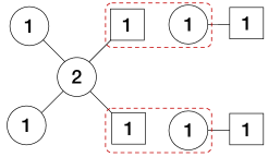
Refer to caption
Refer to caption
Figure 25: Attaching two (1,1)11(1,1) blocks to a (1,0)(2,2)(1,0)102210(1,0)(2,2)(1,0) theory (left) in order to get the D^4subscript^𝐷4\hat{D}_{4} quiver with two framings (right).

At the level of the partition function this operation can be represented in the following form

𝒵~A(a1,a2;tj,ζ1,ζ2)=i=12dmie2πiζimicoshπ(miai)𝒵A(mi;tj),subscript~𝒵𝐴subscript𝑎1subscript𝑎2subscript𝑡𝑗subscript𝜁1subscript𝜁2subscriptsuperscriptproduct2𝑖1𝑑subscript𝑚𝑖superscript𝑒2𝜋𝑖subscript𝜁𝑖subscript𝑚𝑖𝜋subscript𝑚𝑖subscript𝑎𝑖subscript𝒵𝐴subscript𝑚𝑖subscript𝑡𝑗\begin{split}\widetilde{{\cal Z}}_{A}(a_{1},a_{2};{t}_{j},\zeta_{1},\zeta_{2})=\int\prod^{2}_{i=1}dm_{i}\frac{e^{2\pi i\zeta_{i}m_{i}}}{\cosh{\pi(m_{i}-a_{i})}}{\cal Z}_{A}(m_{i};{t}_{j})\,,\end{split} (122)

where 𝒵~A(a1,a2;tj,ζ1,ζ2)subscript~𝒵𝐴subscript𝑎1subscript𝑎2subscript𝑡𝑗subscript𝜁1subscript𝜁2\widetilde{{\cal Z}}_{A}(a_{1},a_{2};{t}_{j},\zeta_{1},\zeta_{2}) is the partition function of the framed D^4subscript^𝐷4\hat{D}_{4} quiver of interest written in terms of the partition function of the (1,0)(2,2)(1,0)102210(1,0)(2,2)(1,0) theory. Note that ζ1,ζ2subscript𝜁1subscript𝜁2\zeta_{1},\zeta_{2} are FI parameters of the attached U(1)𝑈1U(1) nodes and a1,a2subscript𝑎1subscript𝑎2a_{1},a_{2} are the masses of the fundamental hypers charged under those U(1)𝑈1U(1)s.

In order to obtain the correct mirror to this theory, we will need to start with 𝒵~Asubscript~𝒵𝐴\widetilde{{\cal Z}}_{A} and implement S-duality at the level of the partition function in a fashion similar to Dey:2013nf ; Dey:2011pt . To see precisely how this works out, let us rewrite 𝒵~Asubscript~𝒵𝐴\widetilde{{\cal Z}}_{A} in the following manner,

𝒵~A(a1,a2;tj,ζ1,ζ2)=i=12dmiα=12dsαd2s02!1sinhπ(m1m2)i=12e2πiζimicoshπ(miai)×sinhπ(m1m2)sinhπ(s01s02)i,jcoshπ(s0imj)×sinhπ(s01s02)sinhπ(s1s2)i,jcoshπ(s0isj)×α=12e2πisαηαi=12e2πis0iη0sinhπ(s1s2)=i=12dmidmiduidvidzidxdyα=12dsαd2s02!tanhπxe2πix(m1m2)i=12e2πiζimie2πi(mimi)zicoshπ(miai)×(ρ(1)ρi=12e2πiui(s0imρ(i))coshπui)×(ρ(1)ρi=12e2πivi(s0isρ(i))coshπvi)×tanhπye2πiy(s1s2)α=12e2πisαηαi=12e2πis0iη0,subscript~𝒵𝐴subscript𝑎1subscript𝑎2subscript𝑡𝑗subscript𝜁1subscript𝜁2subscriptsuperscriptproduct2𝑖1𝑑subscript𝑚𝑖subscriptsuperscriptproduct2𝛼1𝑑subscript𝑠𝛼superscript𝑑2subscript𝑠021𝜋subscript𝑚1subscript𝑚2subscriptsuperscriptproduct2𝑖1superscript𝑒2𝜋𝑖subscript𝜁𝑖subscript𝑚𝑖𝜋subscript𝑚𝑖subscript𝑎𝑖𝜋subscript𝑚1subscript𝑚2𝜋subscriptsuperscript𝑠10subscriptsuperscript𝑠20subscriptproduct𝑖𝑗𝜋subscriptsuperscript𝑠𝑖0subscript𝑚𝑗𝜋subscriptsuperscript𝑠10subscriptsuperscript𝑠20𝜋subscript𝑠1subscript𝑠2subscriptproduct𝑖𝑗𝜋subscriptsuperscript𝑠𝑖0subscript𝑠𝑗subscriptsuperscriptproduct2𝛼1superscript𝑒2𝜋𝑖subscript𝑠𝛼subscript𝜂𝛼subscriptsuperscriptproduct2𝑖1superscript𝑒2𝜋𝑖subscriptsuperscript𝑠𝑖0subscript𝜂0𝜋subscript𝑠1subscript𝑠2subscriptsuperscriptproduct2𝑖1𝑑subscript𝑚𝑖𝑑subscriptsuperscript𝑚𝑖𝑑subscript𝑢𝑖𝑑subscript𝑣𝑖𝑑subscript𝑧𝑖𝑑𝑥𝑑𝑦subscriptsuperscriptproduct2𝛼1𝑑subscript𝑠𝛼superscript𝑑2subscript𝑠02𝜋𝑥superscript𝑒2𝜋𝑖𝑥subscript𝑚1subscript𝑚2subscriptsuperscriptproduct2𝑖1superscript𝑒2𝜋𝑖subscript𝜁𝑖subscript𝑚𝑖superscript𝑒2𝜋𝑖subscript𝑚𝑖subscriptsuperscript𝑚𝑖subscript𝑧𝑖𝜋subscript𝑚𝑖subscript𝑎𝑖subscript𝜌superscript1𝜌subscriptsuperscriptproduct2𝑖1superscript𝑒2𝜋𝑖subscript𝑢𝑖subscriptsuperscript𝑠𝑖0subscriptsuperscript𝑚𝜌𝑖𝜋subscript𝑢𝑖subscriptsuperscript𝜌superscript1superscript𝜌subscriptsuperscriptproduct2𝑖1superscript𝑒2𝜋𝑖subscript𝑣𝑖subscriptsuperscript𝑠𝑖0subscript𝑠superscript𝜌𝑖𝜋subscript𝑣𝑖𝜋𝑦superscript𝑒2𝜋𝑖𝑦subscript𝑠1subscript𝑠2subscriptsuperscriptproduct2𝛼1superscript𝑒2𝜋𝑖subscript𝑠𝛼subscript𝜂𝛼subscriptsuperscriptproduct2𝑖1superscript𝑒2𝜋𝑖subscriptsuperscript𝑠𝑖0subscript𝜂0\begin{split}&\widetilde{{\cal Z}}_{A}(a_{1},a_{2};{t}_{j},\zeta_{1},\zeta_{2})=\int\prod^{2}_{i=1}dm_{i}\prod^{2}_{\alpha=1}ds_{\alpha}\frac{d^{2}s_{0}}{2!}\frac{1}{\sinh{\pi(m_{1}-m_{2})}}\prod^{2}_{i=1}\frac{e^{2\pi i\zeta_{i}m_{i}}}{\cosh{\pi(m_{i}-a_{i})}}\\ &\times\frac{\sinh{\pi(m_{1}-m_{2})}\sinh{\pi(s^{1}_{0}-s^{2}_{0})}}{\prod_{i,j}\cosh{\pi(s^{i}_{0}-m_{j})}}\times\frac{\sinh{\pi(s^{1}_{0}-s^{2}_{0})}\sinh{\pi(s_{1}-s_{2})}}{\prod_{i,j}\cosh{\pi(s^{i}_{0}-s_{j})}}\times\frac{\prod^{2}_{\alpha=1}e^{2\pi is_{\alpha}\eta_{\alpha}}\prod^{2}_{i=1}e^{2\pi is^{i}_{0}\eta_{0}}}{\sinh{\pi(s_{1}-s_{2})}}\\ &=-\int\prod^{2}_{i=1}dm_{i}dm^{\prime}_{i}du_{i}dv_{i}dz_{i}dxdy\prod^{2}_{\alpha=1}ds_{\alpha}\frac{d^{2}s_{0}}{2!}\tanh{\pi x}\;e^{2\pi ix(m_{1}-m_{2})}\prod^{2}_{i=1}e^{2\pi i\zeta_{i}m_{i}}\frac{e^{2\pi i(m_{i}-m^{\prime}_{i})z_{i}}}{\cosh{\pi(m_{i}-a_{i})}}\\ &\times\left(\sum_{\rho}(-1)^{\rho}\prod^{2}_{i=1}\frac{e^{2\pi iu_{i}(s^{i}_{0}-m^{\prime}_{\rho(i)})}}{\cosh{\pi u_{i}}}\right)\times\left(\sum_{\rho^{\prime}}(-1)^{\rho^{\prime}}\prod^{2}_{i=1}\frac{e^{2\pi iv_{i}(s^{i}_{0}-s_{\rho^{\prime}(i)})}}{\cosh{\pi v_{i}}}\right)\\ &\times\tanh{\pi y}\;e^{2\pi iy(s_{1}-s_{2})}\prod^{2}_{\alpha=1}e^{2\pi is_{\alpha}\eta_{\alpha}}\prod^{2}_{i=1}e^{2\pi is^{i}_{0}\eta_{0}}\,,\end{split} (123)

where ρ,ρ𝜌superscript𝜌\rho,\rho^{\prime} denote permutations over the labels i=1,2𝑖12i=1,2.

Going to the second line from the first, we have used Cauchy determinant identity and Fourier transform of hyperbolic functions to write the partition function in terms of a set of auxiliary variables {x,mi,zi,ui,vi,y}𝑥subscriptsuperscript𝑚𝑖subscript𝑧𝑖subscript𝑢𝑖subscript𝑣𝑖𝑦\{x,m^{\prime}_{i},z_{i},u_{i},v_{i},y\}. For example

sinhπ(m1m2)sinhπ(s01s02)i,jcoshπ(s0imj)=ρ(1)ρ1i=12coshπ(s0imρ(i))=i=12duiρ(1)ρi=12e2πiui(s0imρ(i))coshπui𝜋subscript𝑚1subscript𝑚2𝜋subscriptsuperscript𝑠10subscriptsuperscript𝑠20subscriptproduct𝑖𝑗𝜋subscriptsuperscript𝑠𝑖0subscript𝑚𝑗subscript𝜌superscript1𝜌1subscriptsuperscriptproduct2𝑖1𝜋subscriptsuperscript𝑠𝑖0subscriptsuperscript𝑚𝜌𝑖subscriptsuperscriptproduct2𝑖1𝑑subscript𝑢𝑖subscript𝜌superscript1𝜌subscriptsuperscriptproduct2𝑖1superscript𝑒2𝜋𝑖subscript𝑢𝑖subscriptsuperscript𝑠𝑖0subscriptsuperscript𝑚𝜌𝑖𝜋subscript𝑢𝑖\begin{split}\frac{\sinh{\pi(m_{1}-m_{2})}\sinh{\pi(s^{1}_{0}-s^{2}_{0})}}{\prod_{i,j}\cosh{\pi(s^{i}_{0}-m_{j})}}=&\sum_{\rho}(-1)^{\rho}\frac{1}{\prod^{2}_{i=1}\cosh{\pi(s^{i}_{0}-m^{\prime}_{\rho(i)})}}\\ =&\int\prod^{2}_{i=1}du_{i}\sum_{\rho}(-1)^{\rho}\prod^{2}_{i=1}\frac{e^{2\pi iu_{i}(s^{i}_{0}-m^{\prime}_{\rho(i)})}}{\cosh{\pi u_{i}}}\end{split} (124)

In addition, we used

1sinhπ(m1m2)=i𝑑xtanhπxe2πix(m1m2)1𝜋subscript𝑚1subscript𝑚2𝑖differential-d𝑥𝜋𝑥superscript𝑒2𝜋𝑖𝑥subscript𝑚1subscript𝑚2\begin{split}\frac{1}{\sinh{\pi(m_{1}-m_{2})}}=-i\int dx\;\tanh{\pi x}\;e^{2\pi ix(m_{1}-m_{2})}\end{split} (125)

Implementing S-duality at the level of partition function amounts to carrying out the integration over the original variables {sα,s0i}subscript𝑠𝛼subscriptsuperscript𝑠𝑖0\{s_{\alpha},s^{i}_{0}\} and writing the partition function exclusively in terms of the auxiliary fields. Performing the said integrations followed by some trivial change of variables we have

𝒵~A(a1,a2;tj,ζ1,ζ2)=i=12duidzitanh(πz1)tanh(πu1)(ρ(1)ρi=12e2πiai(ziζi+uρ(i)+ξρ(i))coshπ(ziζi+uρ(i)+ξρ(i)))×(δ(z1+z2)δ(u1+u2)i=12coshπ(ui+ξi)coshπ(ui+ξi+η0)),subscript~𝒵𝐴subscript𝑎1subscript𝑎2subscript𝑡𝑗subscript𝜁1subscript𝜁2subscriptsuperscriptproduct2𝑖1𝑑subscript𝑢𝑖𝑑subscript𝑧𝑖𝜋subscript𝑧1𝜋subscript𝑢1subscript𝜌superscript1𝜌subscriptsuperscriptproduct2𝑖1superscript𝑒2𝜋𝑖subscript𝑎𝑖subscript𝑧𝑖subscript𝜁𝑖subscript𝑢𝜌𝑖subscript𝜉𝜌𝑖𝜋subscript𝑧𝑖subscript𝜁𝑖subscript𝑢𝜌𝑖subscript𝜉𝜌𝑖𝛿subscript𝑧1subscript𝑧2𝛿subscript𝑢1subscript𝑢2subscriptsuperscriptproduct2𝑖1𝜋subscript𝑢𝑖subscript𝜉𝑖𝜋subscript𝑢𝑖subscript𝜉𝑖subscript𝜂0\begin{split}\widetilde{{\cal Z}}_{A}(a_{1},a_{2};{t}_{j},\zeta_{1},\zeta_{2})=&\int\prod^{2}_{i=1}du_{i}dz_{i}\;\tanh{(\pi z_{1})}\tanh{(\pi u_{1})}\left(\sum_{\rho}(-1)^{\rho}\prod^{2}_{i=1}\frac{e^{2\pi ia_{i}(z_{i}-\zeta_{i}+u_{\rho(i)}+\xi_{\rho(i)})}}{\cosh{\pi(z_{i}-\zeta_{i}+u_{\rho(i)}+\xi_{\rho(i)})}}\right)\\ &\times\left(\frac{\delta(z_{1}+z_{2})\delta(u_{1}+u_{2})}{\prod^{2}_{i=1}\cosh{\pi(u_{i}+\xi_{i})}\cosh{\pi(u_{i}+\xi_{i}+\eta_{0})}}\right)\,,\end{split} (126)

where ξ1=η1+η0=t1t3subscript𝜉1subscript𝜂1subscript𝜂0subscript𝑡1subscript𝑡3\xi_{1}=\eta_{1}+\eta_{0}=t_{1}-t_{3} and ξ2=η2+η0=t2t4subscript𝜉2subscript𝜂2subscript𝜂0subscript𝑡2subscript𝑡4\xi_{2}=\eta_{2}+\eta_{0}=t_{2}-t_{4}.

To perform the sum over permutations in 𝒵~Asubscript~𝒵𝐴\widetilde{{\cal Z}}_{A}, we again need to use Cauchy determinant identity. However, this can only be done if the phase is independent of ρ𝜌\rho, which requires that the hypermultiplet masses obey the relation

a1=a2=a.subscript𝑎1subscript𝑎2𝑎a_{1}=a_{2}=a\,. (127)

Imposing this condition and summing over the permutations we obtain

𝒵~A(a;tj,ζ1,ζ2)=d2u2d2z2(sinhπ(z1z2)sinhπ(z1z2ζ1+ζ2)sinhπ(u1u2+ξ1ξ2)sinhπ(u1u2)i,jcoshπ(zi+ujζi+ξj))×(e2πia(ξ1+ξ2ζ1ζ2)δ(z1+z2)δ(u1+u2)i=12coshπ(ui+ξi)coshπ(ui+ξi+η0)cosh(πui)cosh(πzi)).subscript~𝒵𝐴𝑎subscript𝑡𝑗subscript𝜁1subscript𝜁2superscript𝑑2𝑢2superscript𝑑2𝑧2𝜋subscript𝑧1subscript𝑧2𝜋subscript𝑧1subscript𝑧2subscript𝜁1subscript𝜁2𝜋subscript𝑢1subscript𝑢2subscript𝜉1subscript𝜉2𝜋subscript𝑢1subscript𝑢2subscriptproduct𝑖𝑗𝜋subscript𝑧𝑖subscript𝑢𝑗subscript𝜁𝑖subscript𝜉𝑗superscript𝑒2𝜋𝑖𝑎subscript𝜉1subscript𝜉2subscript𝜁1subscript𝜁2𝛿subscript𝑧1subscript𝑧2𝛿subscript𝑢1subscript𝑢2subscriptsuperscriptproduct2𝑖1𝜋subscript𝑢𝑖subscript𝜉𝑖𝜋subscript𝑢𝑖subscript𝜉𝑖subscript𝜂0𝜋subscript𝑢𝑖𝜋subscript𝑧𝑖\begin{split}&\widetilde{{\cal Z}}_{A}(a;{t}_{j},\zeta_{1},\zeta_{2})\\ &=\int\frac{d^{2}u}{2}\frac{d^{2}z}{2}\;\left(\frac{\sinh{\pi(z_{1}-z_{2})}\sinh{\pi(z_{1}-z_{2}-\zeta_{1}+\zeta_{2})}\sinh{\pi(u_{1}-u_{2}+\xi_{1}-\xi_{2})}\sinh{\pi(u_{1}-u_{2})}}{\prod_{i,j}\cosh{\pi(z_{i}+u_{j}-\zeta_{i}+\xi_{j})}}\right)\\ &\times\left(\frac{e^{2\pi ia(\xi_{1}+\xi_{2}-\zeta_{1}-\zeta_{2})}\delta(z_{1}+z_{2})\delta(u_{1}+u_{2})}{\prod^{2}_{i=1}\cosh{\pi(u_{i}+\xi_{i})}\cosh{\pi(u_{i}+\xi_{i}+\eta_{0})}\cosh{(\pi u_{i})}\cosh{(\pi z_{i})}}\right)\,.\end{split} (128)

To interpret the numerator of the first term in parenthesis as the contribution of a 𝒩=2𝒩2\mathcal{N}=2 vector multiplet, we would need

ζ1=ζ2=ζξ1=ξ2=ξ,subscript𝜁1subscript𝜁2𝜁subscript𝜉1subscript𝜉2𝜉\begin{split}&\zeta_{1}=\zeta_{2}=\zeta\\ &\xi_{1}=\xi_{2}=\xi\,,\end{split} (129)

which implies

t1+t4=0,t2+t3=0.formulae-sequencesubscript𝑡1subscript𝑡40subscript𝑡2subscript𝑡30t_{1}+t_{4}=0\,,\quad t_{2}+t_{3}=0\,. (130)

The constraint equations (127) and (129) together imply that the masses and the FI parameters obey the 2subscript2\mathbb{Z}_{2} outer automorphism symmetry of the D^4subscript^𝐷4\hat{D}_{4} quiver. Imposing these constraints, we finally have

𝒵~A(a;tj,ζ)=d2u2d2z2(sinh2π(z1z2)sinh2π(u1u2)i,jcoshπ(zi+ujζ+ξ))×(e4πia(ξζ)δ(z1+z2)δ(u1+u2)i=12coshπ(ui+ξ)coshπ(ui+ξ+η0)cosh(πui)cosh(πzi)).subscript~𝒵𝐴𝑎subscript𝑡𝑗𝜁superscript𝑑2𝑢2superscript𝑑2𝑧2superscript2𝜋subscript𝑧1subscript𝑧2superscript2𝜋subscript𝑢1subscript𝑢2subscriptproduct𝑖𝑗𝜋subscript𝑧𝑖subscript𝑢𝑗𝜁𝜉superscript𝑒4𝜋𝑖𝑎𝜉𝜁𝛿subscript𝑧1subscript𝑧2𝛿subscript𝑢1subscript𝑢2subscriptsuperscriptproduct2𝑖1𝜋subscript𝑢𝑖𝜉𝜋subscript𝑢𝑖𝜉subscript𝜂0𝜋subscript𝑢𝑖𝜋subscript𝑧𝑖\begin{split}\widetilde{{\cal Z}}_{A}(a;{t}_{j},\zeta)=&\int\frac{d^{2}u}{2}\frac{d^{2}z}{2}\;\left(\frac{\sinh^{2}{\pi(z_{1}-z_{2})}\sinh^{2}{\pi(u_{1}-u_{2})}}{\prod_{i,j}\cosh{\pi(z_{i}+u_{j}-\zeta+\xi)}}\right)\\ &\times\left(\frac{e^{4\pi ia(\xi-\zeta)}\delta(z_{1}+z_{2})\delta(u_{1}+u_{2})}{\prod^{2}_{i=1}\cosh{\pi(u_{i}+\xi)}\cosh{\pi(u_{i}+\xi+\eta_{0})}\cosh{(\pi u_{i})}\cosh{(\pi z_{i})}}\right)\,.\end{split} (131)

This is evidently the partition function of a (Sp(1),1)(Sp(1),3)𝑆𝑝11𝑆𝑝13(Sp(1),1)(Sp(1),3) quiver shown in Fig. 22. The mirror map can be read off from the above formula.

M1=t1+t2M2=t1+t22t3M3=0M4=0Mbif=t1t3+ζ.subscript𝑀1subscript𝑡1subscript𝑡2subscript𝑀2subscript𝑡1subscript𝑡22subscript𝑡3subscript𝑀30subscript𝑀40subscript𝑀bifsubscript𝑡1subscript𝑡3𝜁\begin{split}&M_{1}=t_{1}+t_{2}\\ &M_{2}=t_{1}+t_{2}-2t_{3}\\ &M_{3}=0\\ &M_{4}=0\\ &M_{\text{bif}}=t_{1}-t_{3}+\zeta\,.\end{split} (132)

Note that the number of non-zero mass parameters of the B model exactly match with the number of independent FI parameters of the A model.

In order to obtain a generic mirror pair in this class (for rank of the quiver N>4𝑁4N>4) by gauging, we start from a linear quiver (2,2)1(2,0)2(2,2)N3subscript221subscript202subscript22𝑁3(2,2)_{1}(2,0)_{2}\ldots(2,2)_{N-3}. Firstly, one needs to gauge the flavor group U(2)1𝑈subscript21U(2)_{1} as a U(1)×U(1)𝑈1𝑈1U(1)\times U(1). Then the flavor group U(2)N3𝑈subscript2𝑁3U(2)_{N-3} should be split as a U(1)×U(1)𝑈1𝑈1U(1)\times U(1) and a (1,1)11(1,1) quiver must be attached to each U(1)𝑈1U(1) as we did in the D^4subscript^𝐷4\hat{D}_{4} case. The resultant quiver can then be shown to dual to (Sp(1),1)(Sp(1),N1)𝑆𝑝11𝑆𝑝1𝑁1(Sp(1),1)(Sp(1),N-1) using manipulations similar to the example shown above.
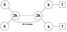
Refer to caption
Refer to caption
Figure 26: An infinite family of affine doubly framed D𝐷D-type quivers with its mirror duals

The details of this computation and the associated mirror map can be found in Dey:2013nf . We leave it to the enthusiastic reader as an exercise to show that, using similar manipulations and attaching (k,1)𝑘1(k,1) blocks as we did above in the case of k=1𝑘1k=1, one can derive the mirror quiver to the doubly framed D^Nsubscript^𝐷𝑁\hat{D}_{N} quiver for generic k𝑘k (Fig. 26) directly.

5 Flavored Ensubscript𝐸𝑛E_{n} and E^nsubscript^𝐸𝑛\hat{E}_{n} Quivers

In this section, we study a few examples of framed Ensubscript𝐸𝑛E_{n} quivers (and their affine extensions) using the framework of Abelian gauging. It was known for some time already Intriligator:1996ex (see also Benini:2010uu ; Chacaltana:2010ks ) that balanced E^nsubscript^𝐸𝑛\hat{E}_{n} quiver theories have non-Lagrangian mirror description and until recently Cremonesi:2013lqa understanding of Higgs branches thereof was limited. The examples we are about to discuss here exclusively deal with framed E𝐸E-type or E^^𝐸\hat{E}-type quivers which have Lagrangian mirrors.

5.1 Framed E6subscript𝐸6E_{6} Theory from Linear Quiver

Consider the mirror pair in Fig. 27 888We are using Bourbaki conventions for numbering the nodes of E𝐸E quiver diagrams. . This mirror pair may be obtained by the abelian gauging technique using S3superscript𝑆3S^{3} partition function in a way similar to the previous sections. The starting point is again a linear quiver pair

A-model:(1,0)(2,0)(3,2)(2,0)(1,0)B-model:(3,6).:A-model1020322010B-model:36\begin{split}&\textbf{A-model}:\;\;(1,0)(2,0)(3,2)(2,0)(1,0)\\ &\textbf{B-model}:\;\;(3,6)\,.\end{split} (133)

We perform the gauging trick on the global U(2)𝑈2U(2) symmetry of the middle node of the left quiver into U(1)𝑈1U(1) global and U(1)𝑈1U(1) gauge. From the perspective of the parameter space, this amounts to fixing one of the momenta, say pμ(3) 1subscriptsuperscript𝑝31𝜇p^{(3)\,1}_{\mu}, which on the mirror side results in taking out the trace part of U(3)𝑈3U(3).

Refer to caption
Refer to caption
Figure 27: E6subscript𝐸6E_{6} quiver with one hypermultiplet on the middle node and its mirror. Red number near the nodes of the E6subscript𝐸6E_{6} quiver enumerate the nodes accruing to the Bourbaki convention. The quiver on the left can be obtained from gluing T(1,1,1)(U(3))subscript𝑇111𝑈3T_{(1,1,1)}(U(3)), T(1,1,1)(U(3))subscript𝑇111𝑈3T_{(1,1,1)}(U(3)), T(2,1)(U(3))subscript𝑇21𝑈3T_{(2,1)}(U(3)) and T(2,1)(U(3))subscript𝑇21𝑈3T_{(2,1)}(U(3)) together via the U(3)𝑈3U(3) group, and the quiver on the right can be realised as as the 6d6𝑑6d (2,0)20(2,0) theory compactifying on a circle times a Riemann sphere with punctures (1,1,1)111(1,1,1), (1,1,1)111(1,1,1), (2,1)21(2,1) and (2,1)21(2,1).

Mirror symmetry dictates that the partition functions of the two linear quivers are related in the following manner up to an overall phase. In Benini:2010uu the same example was considered, however, on the A side the quiver had SU(3)𝑆𝑈3SU(3) group in the middle instead of U(3)𝑈3U(3) with the overall U(1)𝑈1U(1) factorization. We stress again here that our computation is the correct one and only with the democratic overall U(1)𝑈1U(1) quotient the mirror map works correctly.

𝒵A(ma,tα)=𝒵B(Mα,t~a)ma=t~a,a=1,2.tα=Mα,α=1,2,,6formulae-sequencesubscript𝒵𝐴subscript𝑚𝑎subscript𝑡𝛼subscript𝒵𝐵subscript𝑀𝛼subscript~𝑡𝑎subscript𝑚𝑎subscript~𝑡𝑎𝑎12formulae-sequencesubscript𝑡𝛼subscript𝑀𝛼𝛼126\begin{split}&{\cal Z}_{A}(m_{a},t_{\alpha})={\cal Z}_{B}(M_{\alpha},\widetilde{t}_{a})\\ &m_{a}=\widetilde{t}_{a},\;\;a=1,2.\\ &t_{\alpha}=M_{\alpha},\;\;\alpha=1,2,\ldots,6\end{split} (134)

Now consider gauging a single U(1)𝑈1U(1) of the U(2)𝑈2U(2) global symmetry in the A-model linear quiver to obtain the correct framed E6subscript𝐸6E_{6} quiver. The partition function of such a theory is

𝒵~A(ζ1,m2,tα)=𝑑m1e2πiζ1m1𝒵A(ma,tα)=𝑑m1e2πiζ1m1𝒵B(tα,ma)subscript~𝒵𝐴subscript𝜁1subscript𝑚2subscript𝑡𝛼differential-dsubscript𝑚1superscript𝑒2𝜋𝑖subscript𝜁1subscript𝑚1subscript𝒵𝐴subscript𝑚𝑎subscript𝑡𝛼differential-dsubscript𝑚1superscript𝑒2𝜋𝑖subscript𝜁1subscript𝑚1subscript𝒵𝐵subscript𝑡𝛼subscript𝑚𝑎\begin{split}\widetilde{{\cal Z}}_{A}(\zeta_{1},m_{2},t_{\alpha})=&\int dm_{1}e^{2\pi i\zeta_{1}m_{1}}{{\cal Z}}_{A}(m_{a},t_{\alpha})\\ =&\int dm_{1}e^{2\pi i\zeta_{1}m_{1}}{{\cal Z}}_{B}(t_{\alpha},m_{a})\end{split} (135)

where the second equality is a direct consequence of mirror symmetry. Therefore, we have

𝒵~A(ζ1,m2,tα)=𝑑m1d3s3!e2πiζ1m1i=13e2πisi(m1m2)i<jsinh2π(sisj)i=13α=16coshπ(si+tα)=d3s3!δ(s1+s2+s3)i<jsinh2π(sisj)i=13α=16coshπ(si+tαζ13)=𝒵~B(Mα)subscript~𝒵𝐴subscript𝜁1subscript𝑚2subscript𝑡𝛼differential-dsubscript𝑚1superscript𝑑3𝑠3superscript𝑒2𝜋𝑖subscript𝜁1subscript𝑚1subscriptsuperscriptproduct3𝑖1superscript𝑒2𝜋𝑖superscript𝑠𝑖subscript𝑚1subscript𝑚2subscriptproduct𝑖𝑗superscript2𝜋superscript𝑠𝑖superscript𝑠𝑗subscriptsuperscriptproduct3𝑖1subscriptsuperscriptproduct6𝛼1𝜋superscript𝑠𝑖subscript𝑡𝛼superscript𝑑3𝑠3𝛿superscript𝑠1superscript𝑠2superscript𝑠3subscriptproduct𝑖𝑗superscript2𝜋superscript𝑠𝑖superscript𝑠𝑗subscriptsuperscriptproduct3𝑖1subscriptsuperscriptproduct6𝛼1𝜋superscript𝑠𝑖subscript𝑡𝛼subscript𝜁13subscript~𝒵𝐵subscript𝑀𝛼\begin{split}\widetilde{{\cal Z}}_{A}(\zeta_{1},m_{2},t_{\alpha})=&\int dm_{1}\frac{d^{3}s}{3!}\frac{e^{2\pi i\zeta_{1}m_{1}}\prod^{3}_{i=1}e^{2\pi is^{i}(m_{1}-m_{2})}\prod_{i<j}\sinh^{2}{\pi(s^{i}-s^{j})}}{\prod^{3}_{i=1}\prod^{6}_{\alpha=1}\cosh{\pi(s^{i}+t_{\alpha})}}\\ =&\int\frac{d^{3}s}{3!}\frac{\delta(s^{1}+s^{2}+s^{3})\prod_{i<j}\sinh^{2}{\pi(s^{i}-s^{j})}}{\prod^{3}_{i=1}\prod^{6}_{\alpha=1}\cosh{\pi(s^{i}+t_{\alpha}-\frac{\zeta_{1}}{3})}}\\ =&\widetilde{{\cal Z}}_{B}(M_{\alpha})\end{split} (136)

The theory dual to the E6subscript𝐸6E_{6} quiver with a single fundamental hyper can be read off from the partition function above -SU(3)𝑆𝑈3SU(3) with 6 flavors. The mirror map relates the masses of the fundamental hypers of SU(3)𝑆𝑈3SU(3) with the FI parameters of the framed E6subscript𝐸6E_{6} quiver.

Mα=tαζ13,α=1,2,,6formulae-sequencesubscript𝑀𝛼subscript𝑡𝛼subscript𝜁13𝛼126\begin{split}M_{\alpha}=t_{\alpha}-\frac{\zeta_{1}}{3},\;\;\alpha=1,2,\ldots,6\end{split} (137)

As expected, the 6 independent mass parameters of the B-model match with the number of independent parameters of the A-model - 6 parameters {tα}subscript𝑡𝛼\{t_{\alpha}\} with one constraint and ζ1subscript𝜁1\zeta_{1}.

Another way to realize the mirror pairs in Fig. 27 is as follows. The quiver on the left can be obtained from gluing T(1,1,1)(U(3))subscript𝑇111𝑈3T_{(1,1,1)}(U(3)), T(1,1,1)(U(3))subscript𝑇111𝑈3T_{(1,1,1)}(U(3)), T(2,1)(U(3))subscript𝑇21𝑈3T_{(2,1)}(U(3)) and T(2,1)(U(3))subscript𝑇21𝑈3T_{(2,1)}(U(3)) together via the U(3)𝑈3U(3) group, and the mirror quiver on the right can be realised as as the 6d6𝑑6d (2,0)20(2,0) theory compactifying on a circle times a Riemann sphere with punctures (1,1,1)111(1,1,1), (1,1,1)111(1,1,1), (2,1)21(2,1) and (2,1)21(2,1) Benini:2010uu . Indeed, according to Argyres:2007cn and Chacaltana:2010ks ,999the diagram on page 16 of Chacaltana:2010ks such a mirror theory is the SU(3)𝑆𝑈3SU(3) gauge theory with 666 flavours.

5.2 E^7subscript^𝐸7\hat{E}_{7} Theory from Linear Quiver

Now we consider an example of a framed E^7subscript^𝐸7\hat{E}_{7} quiver, see Fig. 28.

Refer to captionRefer to caption
Figure 28: E^7subscript^𝐸7\hat{E}_{7} quiver with one hypermultiplet on the branching node and its mirror.

In order to obtain this mirror pair via Abelian gauging, we start from the following mirror pairs.

A-model:(1,0)(2,0)(3,0)(4,2)(3,0)(2,0)(1,0)B-model:(4,8):A-model10203042302010B-model:48\begin{split}&\textbf{A-model}:\;\;(1,0)(2,0)(3,0)(4,2)(3,0)(2,0)(1,0)\\ &\textbf{B-model}:\;\;(4,8)\end{split} (138)

We perform the gauging trick on the global U(2)𝑈2U(2) symmetry of the middle node of the left quiver into U(1)𝑈1U(1) global and U(1)𝑈1U(1) gauge. From the perspective of the parameter space, this amounts to fixing one of the momenta, which on the mirror side results in taking out the trace part of U(4)𝑈4U(4).

Mirror symmetry dictates that the partition functions of the two linear quivers are related in the following manner up to an overall phase.

𝒵A(ma,tα)=𝒵B(Mα,t~a)ma=t~a,a=1,2.tα=Mα,α=1,2,,8formulae-sequencesubscript𝒵𝐴subscript𝑚𝑎subscript𝑡𝛼subscript𝒵𝐵subscript𝑀𝛼subscript~𝑡𝑎subscript𝑚𝑎subscript~𝑡𝑎𝑎12formulae-sequencesubscript𝑡𝛼subscript𝑀𝛼𝛼128\begin{split}&{\cal Z}_{A}(m_{a},t_{\alpha})={\cal Z}_{B}(M_{\alpha},\widetilde{t}_{a})\\ &m_{a}=\widetilde{t}_{a},\;\;a=1,2.\\ &t_{\alpha}=M_{\alpha},\;\;\alpha=1,2,\ldots,8\end{split} (139)

Now consider gauging a single U(1)𝑈1U(1) of the U(2)𝑈2U(2) global symmetry in the A-model linear quiver to obtain the correct framed E^7subscript^𝐸7\hat{E}_{7} quiver. The partition function of such a theory is

𝒵~A(ζ1,m2,tα)=𝑑m1e2πiζ1m1𝒵A(ma,tα)=𝑑m1e2πiζ1m1𝒵B(tα,ma)subscript~𝒵𝐴subscript𝜁1subscript𝑚2subscript𝑡𝛼differential-dsubscript𝑚1superscript𝑒2𝜋𝑖subscript𝜁1subscript𝑚1subscript𝒵𝐴subscript𝑚𝑎subscript𝑡𝛼differential-dsubscript𝑚1superscript𝑒2𝜋𝑖subscript𝜁1subscript𝑚1subscript𝒵𝐵subscript𝑡𝛼subscript𝑚𝑎\begin{split}\widetilde{{\cal Z}}_{A}(\zeta_{1},m_{2},t_{\alpha})=&\int dm_{1}e^{2\pi i\zeta_{1}m_{1}}{{\cal Z}}_{A}(m_{a},t_{\alpha})\\ =&\int dm_{1}e^{2\pi i\zeta_{1}m_{1}}{{\cal Z}}_{B}(t_{\alpha},m_{a})\end{split} (140)

where the second equality is a direct consequence of mirror symmetry. Therefore, we have

𝒵~A(ζ1,m2,tα)=𝑑m1d4s3!e2πiζ1m1i=14e2πisi(m1m2)i<jsinh2π(sisj)i=14α=18coshπ(si+tα)=d4s3!δ(s1+s2+s3+s4)i<jsinh2π(sisj)i=13α=16coshπ(si+tαζ14)=𝒵~B(Mα)subscript~𝒵𝐴subscript𝜁1subscript𝑚2subscript𝑡𝛼differential-dsubscript𝑚1superscript𝑑4𝑠3superscript𝑒2𝜋𝑖subscript𝜁1subscript𝑚1subscriptsuperscriptproduct4𝑖1superscript𝑒2𝜋𝑖superscript𝑠𝑖subscript𝑚1subscript𝑚2subscriptproduct𝑖𝑗superscript2𝜋superscript𝑠𝑖superscript𝑠𝑗subscriptsuperscriptproduct4𝑖1subscriptsuperscriptproduct8𝛼1𝜋superscript𝑠𝑖subscript𝑡𝛼superscript𝑑4𝑠3𝛿superscript𝑠1superscript𝑠2superscript𝑠3superscript𝑠4subscriptproduct𝑖𝑗superscript2𝜋superscript𝑠𝑖superscript𝑠𝑗subscriptsuperscriptproduct3𝑖1subscriptsuperscriptproduct6𝛼1𝜋superscript𝑠𝑖subscript𝑡𝛼subscript𝜁14subscript~𝒵𝐵subscript𝑀𝛼\begin{split}\widetilde{{\cal Z}}_{A}(\zeta_{1},m_{2},t_{\alpha})=&\int dm_{1}\frac{d^{4}s}{3!}\frac{e^{2\pi i\zeta_{1}m_{1}}\prod^{4}_{i=1}e^{2\pi is^{i}(m_{1}-m_{2})}\prod_{i<j}\sinh^{2}{\pi(s^{i}-s^{j})}}{\prod^{4}_{i=1}\prod^{8}_{\alpha=1}\cosh{\pi(s^{i}+t_{\alpha})}}\\ =&\int\frac{d^{4}s}{3!}\frac{\delta(s^{1}+s^{2}+s^{3}+s^{4})\prod_{i<j}\sinh^{2}{\pi(s^{i}-s^{j})}}{\prod^{3}_{i=1}\prod^{6}_{\alpha=1}\cosh{\pi(s^{i}+t_{\alpha}-\frac{\zeta_{1}}{4})}}\\ =&\widetilde{{\cal Z}}_{B}(M_{\alpha})\end{split} (141)

The theory dual to the E^7subscript^𝐸7\hat{E}_{7} quiver with a single fundamental hyper in the middle node can now be read off from the partition function above - a SU(4)𝑆𝑈4SU(4) with 8 flavors. The mirror map relates the masses of the fundamental hypers of SU(4)𝑆𝑈4SU(4) with the FI parameters of the framed E^7subscript^𝐸7\hat{E}_{7} quiver.

Mα=tαζ14,α=1,2,,8formulae-sequencesubscript𝑀𝛼subscript𝑡𝛼subscript𝜁14𝛼128\begin{split}M_{\alpha}=t_{\alpha}-\frac{\zeta_{1}}{4},\;\;\alpha=1,2,\ldots,8\end{split} (142)

As expected, the 8 independent mass parameters of the B-model match with the number of independent parameters of the A-model - 8 parameters {tα}subscript𝑡𝛼\{t_{\alpha}\} with one constraint and ζ1subscript𝜁1\zeta_{1}.

Another way to realize the mirror pairs in Fig. 28 is as follows. The quiver on the left can be obtained from gluing T(1,1,1,1)(U(4))subscript𝑇1111𝑈4T_{(1,1,1,1)}(U(4)), T(1,1,1,1)(U(4))subscript𝑇1111𝑈4T_{(1,1,1,1)}(U(4)), T(3,1)(U(4))subscript𝑇31𝑈4T_{(3,1)}(U(4)) and T(3,1)(U(4))subscript𝑇31𝑈4T_{(3,1)}(U(4)) together via the U(4)𝑈4U(4) group, and the quiver on the right can be realized as as the 6d6𝑑6d (2,0)20(2,0) theory compactifying on a circle times a Riemann sphere with punctures (1,1,1,1)1111(1,1,1,1), (1,1,1,1)1111(1,1,1,1), (3,1)31(3,1) and (3,1)31(3,1) Benini:2010uu . Indeed, according to Chacaltana:2010ks , such a mirror theory is the SU(4)𝑆𝑈4SU(4) gauge theory with 888 flavors.

5.3 E^8subscript^𝐸8\hat{E}_{8} Theory from Linear Quiver

Similarly we can obtain extended E8subscript𝐸8E_{8} graphs by employing Abelian gauging on the following mirror pair of linear quivers

(2,0)(4,0)(6,3)(5,0)(4,0)(3,0)(2,0)(1,0)(6,9)(3,0).20406350403020106930(2,0)(4,0)(6,3)(5,0)(4,0)(3,0)(2,0)(1,0)\qquad\qquad(6,9)(3,0)\,. (143)

By gauging a single U(1)𝑈1U(1) factor on the (6,3)63(6,3) node of the left quiver above we derive the new mirror pair, see Fig. 29.

Refer to caption
Refer to caption
Figure 29: E^8subscript^𝐸8\hat{E}_{8} quiver with one hypermultiplet on the bifurcating node and its mirror.

Gauging out another U(1)𝑈1U(1) on the bifurcating node of the left quiver in Fig. 29 will transform the mirror dual to (SU(6),9)(SU(3),0)𝑆𝑈69𝑆𝑈30(SU(6),9)(SU(3),0). Finally, gauging out the remaining U(1)𝑈1U(1) global symmetry on the same node does not change the mirror, but the A-model quiver turns into the one depicted in Fig. 30. Recall that the overall U(1)𝑈1U(1) gauge factor decouples.

Refer to caption
Figure 30: The result of complete Abelian gauging on the U(6)𝑈6U(6) node. This quiver is mirror to another quiver theory: (SU(6),9)(SU(3),0)𝑆𝑈69𝑆𝑈30(SU(6),9)(SU(3),0).

It is instructive at this point to consider the six dimensional realization of the mirror theory of Fig. 30. The quiver in Fig. 30 can be constructed by gluing T(23)(U(6))subscript𝑇superscript23𝑈6T_{(2^{3})}(U(6)), 3 copies of T(16)(U(6))subscript𝑇superscript16𝑈6T_{(1^{6})}(U(6)), and T(5,1)(U(6))subscript𝑇51𝑈6T_{(5,1)}(U(6)) together via the U(6)𝑈6U(6) group and modding out by an overall U(1)𝑈1U(1). According to Benini:2010uu , the mirror theory can be realised from the 6d6𝑑6d (2,0)20(2,0) theories compactified on a Riemann sphere with the following punctures: (16)superscript16(1^{6}), 3 copies of (5,1)51(5,1) and (2,2,2)222(2,2,2). We can decompose the Riemann sphere as in Fig. 31.
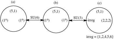
Refer to caption
Figure 31: The puncture decomposition of the mirror theory of Fig. 30. The sequence in the round brackets corresponds to the Young diagram of the puncture, whereas the sequence in the curly bracket corresponds to the pole structure used in Chacaltana:2010ks . The maximal puncture (16)superscript16(1^{6}) has the pole structure {1,2,3,4,5}12345\{1,2,3,4,5\}, the minimal puncture (5,1)51(5,1) has the pole structure {1,1,1,1,1}11111\{1,1,1,1,1\}, and the puncture (2,2,2)222(2,2,2) has the pole structure {1,2,2,3,4}12234\{1,2,2,3,4\}. The pole structure of the irregular puncture “irreg” is indicated in the figure.

Let us follow the prescription in Chacaltana:2010ks . The gauge group associated with the cylinder connecting two maximal punctures give rise to the gauge group SU(6)𝑆𝑈6SU(6), whereas that associated with the cylinder connecting the maximal puncture and the irregular puncture has rank 222. There are two possibilities for the latter; it is either SU(3)𝑆𝑈3SU(3) or Sp(2)𝑆𝑝2Sp(2). In order to determine this, we need to compute the number of hypermultiplets associated with each fixture using Eq. (10) of Chacaltana:2010ks : fixtures (a)𝑎(a) and (b)𝑏(b) each contains 36 hypermultiplets and fixture (c)𝑐(c) contains zero hypermultiplet. Hence we conclude that the gauge group associated with the cylinder connecting (b)𝑏(b) and (c)𝑐(c) is SU(3)𝑆𝑈3SU(3) with the following matter content:

Fixture # hypers SU(6)𝑆𝑈6SU(6) SU(3)𝑆𝑈3SU(3)
(a)𝑎(a) 6 6 1
(b)𝑏(b) 1 6 3
3 6 1
(c)𝑐(c) - - -
Table 5: Matter content of the configuration in Fig. 31.

The quiver diagram associated with this construction is therefore

(144)

Equivalently, this is

(145)

as obtained using the Abelian gauging procedure.

6 Non-Abelian Gauging: Mirrors of Sp(Nc)𝑆𝑝subscript𝑁𝑐Sp(N_{c}) Theories

In this final section we discuss the construction of mirror duals to Sp(Nc)𝑆𝑝subscript𝑁𝑐Sp(N_{c}) 3d theories with Nfsubscript𝑁𝑓N_{f} flavors by studying parameter spaces of vacua and computing partition functions on S3superscript𝑆3S^{3} for these theories. From the discussion of Hanany:1999sj and Feng:2000eq we know that brane construction of mirror duals may involve O5-planes or O3-planes. In this paper, we focus on the mirror duals whose brane construction only involves O5 planes; we will refer to those as the “O5 mirrors”.

6.1 Brane Construction and S-duality

We have already studied Sp(1)SU(2)similar-to-or-equals𝑆𝑝1𝑆𝑈2Sp(1)\simeq SU(2) theories earlier in the paper (see e.g. Sec. 4.1), so let us immediately proceed to more complicated examples. We will soon see that in order to understand higher rank Sp𝑆𝑝Sp theories starting from linear quivers one has to perform the non-Abelian gauging as opposed to the Abelian gauging which we have used thus far. In this section we shall elaborate in great details on Sp(2)𝑆𝑝2Sp(2) gauge theory with six flavors.

The brane configuration of the Sp(2)𝑆𝑝2Sp(2) theory with 666 flavors involving an O5-plane is presented in Fig. 32 (see Hanany:1999sj for details).
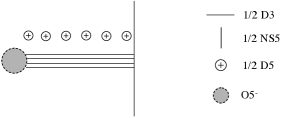
Refer to caption
Figure 32: The brane configuration of Sp(2)𝑆𝑝2Sp(2) with 666 flavors involving an O5-plane.

Let us apply the S-duality to the brane construction from Fig. 32. Upon the S-duality the D5-branes become NS5-branes and vice versa. The O5𝑂superscript5O5^{-} plane becomes the ON𝑂superscript𝑁ON^{-} plane. After all, the S-dual brane configurations is given in Fig. 33.
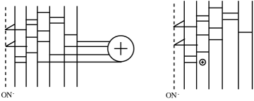
Refer to caption
Figure 33: The brane configurations of the mirror theory of Sp(2)𝑆𝑝2Sp(2) with 666 flavors involving an O5-plane. The notation is the same as Fig. 32, with the dashed vertical line being an ON𝑂superscript𝑁ON^{-} plane. On the left the S-duality is directly applied to Fig. 32, with the D3-branes reconnected according to the s𝑠s-rule such that the number of D3-branes at each interval is preserved. On the right the D5-brane is moved inside so no D3 branes end on it; in this configuration the quiver data can be read off from this diagram.

The quiver of the mirror theory for our problem can be read off directly from the right diagram of Fig. 33; this is depicted in Fig. 34.

Refer to caption
Figure 34: The quiver diagram of a mirror theory of Sp(2)𝑆𝑝2Sp(2) with 666 flavors. The Coulomb branch of this theory is 141414 quanternionic dimensional. The Higgs branch of this theory is 2-quanternionic dimensional.

6.2 Parameter Space Description

Let us now try to derive the mirror quiver for Sp(2)𝑆𝑝2Sp(2) theory with six flavors depicted in Fig. 34 from parameter spaces of linear quivers. These linear quivers are the following (see top row in Fig. 35)

A-model:(2,0)(4,3)(3,0)(2,0)(1,0)A-model:2043302010\displaystyle\textbf{A-model:}\quad(2,0)(4,3)(3,0)(2,0)(1,0)
B-model:(4,6)(2,0)B-model:4620\displaystyle\textbf{B-model:}\quad(4,6)(2,0)\, (146)
Refer to caption
Refer to caption
Figure 35: Mirror pairs before (a𝑎a and b𝑏b) and after (asuperscript𝑎a^{\prime} and bsuperscript𝑏b^{\prime}) the gauging. Dimensions of Coulomb and Higgs branches for the A-models (left) are 121212 and 666 for the top quiver and 141414 and 222 for the bottom quiver.

We then gauge the U(2)𝑈2U(2) subgroup of the U(3)𝑈3U(3) global symmetry on the second node of the A-quiver. This procedure leaves behind U(1)𝑈1U(1) flavor symmetry. Now we need to understand the consequences of gauging on the mirror side. We see that the dimension of the Higgs branch of the bottom-left quiver in Fig. 35 has decreased by 22=4superscript2242^{2}=4, therefore we expect the same to happen for the Coulomb branch of the mirror quiver. Also adding a U(2)𝑈2U(2) gauge node on the A-side increases its Coulomb branch dimension by two, therefore the Higgs branch of the mirror has to be fourteen-dimensional. Clearly the Sp(2)𝑆𝑝2Sp(2) theory with six flavors or with SO(12)𝑆𝑂12SO(12) global symmetry (bottom-right of Fig. 35) is a good candidate since the dimensions of branches match perfectly. However, matching of the dimensions alone is simply not enough to claim victory and a robust derivation of our result is due.

Note that in Fig. 35 quiver (asuperscript𝑎a^{\prime}) can be constructed by gluing T(2,2)(U(4))subscript𝑇22𝑈4T_{(2,2)}(U(4)), T(2,2)(U(4))subscript𝑇22𝑈4T_{(2,2)}(U(4)), T(3,1)(U(4))subscript𝑇31𝑈4T_{(3,1)}(U(4)) and T(1,1,1,1)(U(4))subscript𝑇1111𝑈4T_{(1,1,1,1)}(U(4)) via the U(4)𝑈4U(4) group and modding out by the overall U(1)𝑈1U(1); its mirror Benini:2010uu , quiver (bsuperscript𝑏b^{\prime}), can be realized as the 6d6𝑑6d (2,0)20(2,0) theory compactified on S1superscript𝑆1S^{1} times a Riemann surface with punctures (2,2)22(2,2), (2,2)22(2,2), (3,1)31(3,1) and (1,1,1,1)1111(1,1,1,1). Note also that this particular theory belongs to the classification of Chacaltana:2010ks 101010See top diagram on page 22 of of Chacaltana:2010ks . However, Chacaltana:2010ks classifies theories only up to rank four, whereas here we are interested in constructing mirrors for any Ncsubscript𝑁𝑐N_{c} and Nfsubscript𝑁𝑓N_{f}.

Let us begin with the Bethe equations for the original linear quivers on top of Fig. 35. Vacua equations of the U(4)𝑈4U(4) node of the A-model quiver in (146) read

τ3τ2a=13ησi(2)μa(2)ημa(2)σi(2)a=12ησi(2)σa(1)ησa(1)σi(2)ji4ησi(2)η1σj(2)ησj(2)η1σi(2)a=13ησi(2)σa(3)ησa(3)σi(2)subscript𝜏3subscript𝜏2superscriptsubscriptproduct𝑎13𝜂subscriptsuperscript𝜎2𝑖subscriptsuperscript𝜇2𝑎𝜂subscriptsuperscript𝜇2𝑎subscriptsuperscript𝜎2𝑖superscriptsubscriptproduct𝑎12𝜂subscriptsuperscript𝜎2𝑖subscriptsuperscript𝜎1𝑎𝜂subscriptsuperscript𝜎1𝑎subscriptsuperscript𝜎2𝑖superscriptsubscriptproduct𝑗𝑖4𝜂subscriptsuperscript𝜎2𝑖superscript𝜂1subscriptsuperscript𝜎2𝑗𝜂subscriptsuperscript𝜎2𝑗superscript𝜂1subscriptsuperscript𝜎2𝑖superscriptsubscriptproduct𝑎13𝜂subscriptsuperscript𝜎2𝑖subscriptsuperscript𝜎3𝑎𝜂subscriptsuperscript𝜎3𝑎subscriptsuperscript𝜎2𝑖\displaystyle\frac{\tau_{3}}{\tau_{2}}\prod_{a=1}^{3}\frac{\eta\sigma^{(2)}_{i}-\mu^{(2)}_{a}}{\eta\mu^{(2)}_{a}-\sigma^{(2)}_{i}}\cdot\prod_{a=1}^{2}\frac{\eta\sigma^{(2)}_{i}-\sigma^{(1)}_{a}}{\eta\sigma^{(1)}_{a}-\sigma^{(2)}_{i}}\cdot\prod_{j\neq i}^{4}\frac{\eta\sigma^{(2)}_{i}-\eta^{-1}\sigma^{(2)}_{j}}{\eta\sigma^{(2)}_{j}-\eta^{-1}\sigma^{(2)}_{i}}\cdot\prod_{a=1}^{3}\frac{\eta\sigma^{(2)}_{i}-\sigma^{(3)}_{a}}{\eta\sigma^{(3)}_{a}-\sigma^{(2)}_{i}} =1,absent1\displaystyle=1\,, (147)

together with the corresponding momenta

pμ(2)a=τ1τ2j=14ημaσj(2)ησj(2)μa,a=1,2,3.formulae-sequencesuperscriptsubscript𝑝𝜇2𝑎subscript𝜏1subscript𝜏2superscriptsubscriptproduct𝑗14𝜂subscript𝜇𝑎subscriptsuperscript𝜎2𝑗𝜂subscriptsuperscript𝜎2𝑗subscript𝜇𝑎𝑎123p_{\mu}^{(2)\,a}=\tau_{1}\tau_{2}\prod_{j=1}^{4}\frac{\eta\mu_{a}-\sigma^{(2)}_{j}}{\eta\sigma^{(2)}_{j}-\mu_{a}}\,,\quad a=1,2,3\,. (148)

After the gauging an extra node with U(2)𝑈2U(2) gauge group is added to the quiver, let’s call it 00th node. Vacua equations for this node read

j=14ησa(0)σj(2)ησj(2)σa(0)baησa(0)η1σb(0)ησb(0)η1σa(0)=1,a=1,2.formulae-sequencesuperscriptsubscriptproduct𝑗14𝜂subscriptsuperscript𝜎0𝑎subscriptsuperscript𝜎2𝑗𝜂subscriptsuperscript𝜎2𝑗subscriptsuperscript𝜎0𝑎subscriptproduct𝑏𝑎𝜂subscriptsuperscript𝜎0𝑎superscript𝜂1subscriptsuperscript𝜎0𝑏𝜂subscriptsuperscript𝜎0𝑏superscript𝜂1subscriptsuperscript𝜎0𝑎1𝑎12\prod_{j=1}^{4}\frac{\eta\sigma^{(0)}_{a}-\sigma^{(2)}_{j}}{\eta\sigma^{(2)}_{j}-\sigma^{(0)}_{a}}\cdot\prod_{b\neq a}\frac{\eta\sigma^{(0)}_{a}-\eta^{-1}\sigma^{(0)}_{b}}{\eta\sigma^{(0)}_{b}-\eta^{-1}\sigma^{(0)}_{a}}=1\,,\quad a=1,2\,. (149)

If we multiply the above two equations for a=1𝑎1a=1 and a=2𝑎2a=2 we immediately arrive to the following constraint pσ(0) 1pσ(0) 2=1superscriptsubscript𝑝𝜎01superscriptsubscript𝑝𝜎021p_{\sigma}^{(0)\,1}p_{\sigma}^{(0)\,2}=1 which can be also written as

pμ(2) 1pμ(2) 2=1,superscriptsubscript𝑝𝜇21superscriptsubscript𝑝𝜇221p_{\mu}^{(2)\,1}p_{\mu}^{(2)\,2}=1\,, (150)

if we relabel σ(0)superscript𝜎0\sigma^{(0)}s with μ𝜇\mus.

Meanwhile, on the mirror side we get

τ2τ1a=16η1σi(1)μa(1)η1μa(1)σi(1)ji4ησi(1)η1σj(1)ησj(1)η1σi(1)a=12η1σi(1)σa(2)η1σa(2)σi(1)subscriptsuperscript𝜏2subscriptsuperscript𝜏1superscriptsubscriptproduct𝑎16superscript𝜂1subscriptsuperscript𝜎1𝑖subscriptsuperscript𝜇1𝑎superscript𝜂1subscriptsuperscript𝜇1𝑎subscriptsuperscript𝜎1𝑖superscriptsubscriptproduct𝑗𝑖4𝜂subscriptsuperscript𝜎1𝑖superscript𝜂1subscriptsuperscript𝜎1𝑗𝜂subscriptsuperscript𝜎1𝑗superscript𝜂1subscriptsuperscript𝜎1𝑖superscriptsubscriptproduct𝑎12superscript𝜂1subscriptsuperscript𝜎1𝑖subscriptsuperscript𝜎2𝑎superscript𝜂1subscriptsuperscript𝜎2𝑎subscriptsuperscript𝜎1𝑖\displaystyle\frac{\tau^{\vee}_{2}}{\tau^{\vee}_{1}}\prod_{a=1}^{6}\frac{\eta^{-1}\sigma^{\vee\,(1)}_{i}-\mu^{\vee\,(1)}_{a}}{\eta^{-1}\mu^{\vee\,(1)}_{a}-\sigma^{\vee\,(1)}_{i}}\cdot\prod_{j\neq i}^{4}\frac{\eta\sigma^{\vee\,(1)}_{i}-\eta^{-1}\sigma^{\vee\,(1)}_{j}}{\eta\sigma^{\vee\,(1)}_{j}-\eta^{-1}\sigma^{\vee\,(1)}_{i}}\cdot\prod_{a=1}^{2}\frac{\eta^{-1}\sigma^{\vee\,(1)}_{i}-\sigma^{\vee\,(2)}_{a}}{\eta^{-1}\sigma^{\vee\,(2)}_{a}-\sigma^{\vee\,(1)}_{i}} =1,absent1\displaystyle=1\,,
τ3τ2a=14η1σi(2)σa(1)η1σa(1)σi(2)ji2η1σi(2)ησj(2)η1σj(2)ησi(2)subscriptsuperscript𝜏3subscriptsuperscript𝜏2superscriptsubscriptproduct𝑎14superscript𝜂1subscriptsuperscript𝜎2𝑖subscriptsuperscript𝜎1𝑎superscript𝜂1subscriptsuperscript𝜎1𝑎subscriptsuperscript𝜎2𝑖superscriptsubscriptproduct𝑗𝑖2superscript𝜂1subscriptsuperscript𝜎2𝑖𝜂subscriptsuperscript𝜎2𝑗superscript𝜂1subscriptsuperscript𝜎2𝑗𝜂subscriptsuperscript𝜎2𝑖\displaystyle\frac{\tau^{\vee}_{3}}{\tau^{\vee}_{2}}\prod_{a=1}^{4}\frac{\eta^{-1}\sigma^{\vee\,(2)}_{i}-\sigma^{\vee\,(1)}_{a}}{\eta^{-1}\sigma^{\vee\,(1)}_{a}-\sigma^{\vee\,(2)}_{i}}\cdot\prod_{j\neq i}^{2}\frac{\eta^{-1}\sigma^{\vee\,(2)}_{i}-\eta\sigma^{\vee\,(2)}_{j}}{\eta^{-1}\sigma^{\vee\,(2)}_{j}-\eta\sigma^{\vee\,(2)}_{i}} =1.absent1\displaystyle=1\,. (151)

The mirror analogue of (150) is

pτ 1pτ 2=1,superscriptsubscript𝑝𝜏1superscriptsubscript𝑝𝜏21p_{\tau}^{\vee\,1}p_{\tau}^{\vee\,2}=1\,, (152)

or

τ1(τ2)21σ1(2)σ2(2)=1.subscriptsuperscript𝜏1superscriptsubscriptsuperscript𝜏221subscriptsuperscript𝜎21subscriptsuperscript𝜎221\tau^{\vee}_{1}(\tau^{\vee}_{2})^{2}\frac{1}{\sigma^{\vee\,(2)}_{1}\sigma^{\vee\,(2)}_{2}}=1\,. (153)

The latter condition, up to a constant, (which we shall fix soon) provides an embedding of Sp(1)U(2)𝑆𝑝1𝑈2Sp(1)\subset U(2) for the second node of the B-side quiver.

Note that there is an ambiguity in the choice of (152) which is due to the breaking of the U(3)𝑈3U(3) flavor symmetry on the A side, in other words, one needs to chose which masses (or FI terms on the mirror side) to pick. For a different choice of masses, say μ2subscript𝜇2\mu_{2} and μ3subscript𝜇3\mu_{3} (152) would imply

τ1τ21σ1(1)σ2(1)σ3(1)σ4(1)=1subscriptsuperscript𝜏1subscriptsuperscript𝜏21subscriptsuperscript𝜎11subscriptsuperscript𝜎12subscriptsuperscript𝜎13subscriptsuperscript𝜎141\tau^{\vee}_{1}\tau^{\vee}_{2}\frac{1}{\sigma^{\vee\,(1)}_{1}\sigma^{\vee\,(1)}_{2}\sigma^{\vee\,(1)}_{3}\sigma^{\vee\,(1)}_{4}}=1\, (154)

instead. In order to provide the remaining constraint to ensure the projection of U(4)𝑈4U(4) onto Sp(2)𝑆𝑝2Sp(2) we need to solve Bethe equations and express the solution in terms of momenta (148). Thus we put

σ1(2)=ησ3(1)=ησ2(1)σ2(2)=ησ4(1)=ησ1(1),formulae-sequencesubscriptsuperscript𝜎21𝜂subscriptsuperscript𝜎13𝜂subscriptsuperscript𝜎12subscriptsuperscript𝜎22𝜂subscriptsuperscript𝜎14𝜂subscriptsuperscript𝜎11\sigma^{\vee\,(2)}_{1}=\eta\sigma^{\vee\,(1)}_{3}=\frac{\eta}{\sigma^{\vee\,(1)}_{2}}\,\quad\sigma^{\vee\,(2)}_{2}=\eta\sigma^{\vee\,(1)}_{4}=\frac{\eta}{\sigma^{\vee\,(1)}_{1}}\,, (155)

and observe that the first equation of (6.2) telescopes down to the Bethe equation for Sp(2)𝑆𝑝2Sp(2) theory with six flavors.

In general, if one splits a U(2N+1)𝑈2𝑁1U(2N+1) flavor symmetry on the A side into two U(N)𝑈𝑁U(N) gauge groups and U(1)𝑈1U(1) global symmetry, one imposes N𝑁N constraints in total on momenta pμasuperscriptsubscript𝑝𝜇𝑎p_{\mu}^{a}. Those constraints, translated into the mirror side provide a canonical embedding of Sp(N)𝑆𝑝𝑁Sp(N) gauge group into U(2N)𝑈2𝑁U(2N) group which appeared in the original mirror construction.

6.3 Partition Function Description

Let us now derive the mirror of Sp(2)𝑆𝑝2Sp(2) with 666 flavors using the technique of non-Abelian gauging using, as before, the S3superscript𝑆3S^{3} partition function as a tool. We shall see that working with partition functions will turn out to be a very powerful tool and can be used in gauging of arbitrary quiver theories.

Consider again the pair of mirror quivers (146). Their partition functions read as follows

𝒵A(ma,tα)=d2s12!d4s24!i<jsinh2π(s1is1j)p<lsinh2π(s2ps2l)i,pcoshπ(s1is2p)pa=13coshπ(s2pma)×i=12e2πis1i(t1t2)p=14e2πis2p(t2t3)𝒵T(U(4))(s2p;t3,t4,t5,t6),subscript𝒵𝐴subscript𝑚𝑎subscript𝑡𝛼superscript𝑑2subscript𝑠12superscript𝑑4subscript𝑠24subscriptproduct𝑖𝑗superscript2𝜋subscriptsuperscript𝑠𝑖1subscriptsuperscript𝑠𝑗1subscriptproduct𝑝𝑙superscript2𝜋subscriptsuperscript𝑠𝑝2subscriptsuperscript𝑠𝑙2subscriptproduct𝑖𝑝𝜋subscriptsuperscript𝑠𝑖1subscriptsuperscript𝑠𝑝2subscriptproduct𝑝subscriptsuperscriptproduct3𝑎1𝜋subscriptsuperscript𝑠𝑝2subscript𝑚𝑎subscriptsuperscriptproduct2𝑖1superscript𝑒2𝜋𝑖subscriptsuperscript𝑠𝑖1subscript𝑡1subscript𝑡2subscriptsuperscriptproduct4𝑝1superscript𝑒2𝜋𝑖subscriptsuperscript𝑠𝑝2subscript𝑡2subscript𝑡3subscript𝒵𝑇𝑈4subscriptsuperscript𝑠𝑝2subscript𝑡3subscript𝑡4subscript𝑡5subscript𝑡6\begin{split}{\cal Z}_{A}\left(m_{a},t_{\alpha}\right)&=\int\frac{d^{2}s_{1}}{2!}\frac{d^{4}s_{2}}{4!}\frac{\prod_{i<j}\sinh^{2}{\pi(s^{i}_{1}-s^{j}_{1})}\prod_{p<l}\sinh^{2}{\pi(s^{p}_{2}-s^{l}_{2})}}{\prod_{i,p}\cosh{\pi(s^{i}_{1}-{s}^{p}_{2})}\prod_{p}\prod^{3}_{a=1}\cosh{\pi(s^{p}_{2}-m_{a})}}\\ &\times\prod^{2}_{i=1}e^{2\pi is^{i}_{1}(t_{1}-t_{2})}\prod^{4}_{p=1}e^{2\pi is^{p}_{2}(t_{2}-t_{3})}{\cal Z}_{T(U(4))}\left(s^{p}_{2};t_{3},t_{4},t_{5},t_{6}\right)\,,\end{split} (156)
𝒵B(Mα,t~a)=d2s12!d4s24!i<jsinh2π(s1is1j)p<lsinh2π(s2ps2l)i,pcoshπ(s1is2p)pα=16coshπ(s2pMα)×i=12e2πis1i(t~1t~2)p=14e2πis2p(t~2t~3).subscript𝒵𝐵subscript𝑀𝛼subscript~𝑡𝑎superscript𝑑2subscript𝑠12superscript𝑑4subscript𝑠24subscriptproduct𝑖𝑗superscript2𝜋subscriptsuperscript𝑠𝑖1subscriptsuperscript𝑠𝑗1subscriptproduct𝑝𝑙superscript2𝜋subscriptsuperscript𝑠𝑝2subscriptsuperscript𝑠𝑙2subscriptproduct𝑖𝑝𝜋subscriptsuperscript𝑠𝑖1subscriptsuperscript𝑠𝑝2subscriptproduct𝑝subscriptsuperscriptproduct6𝛼1𝜋subscriptsuperscript𝑠𝑝2subscript𝑀𝛼subscriptsuperscriptproduct2𝑖1superscript𝑒2𝜋𝑖subscriptsuperscript𝑠𝑖1subscript~𝑡1subscript~𝑡2subscriptsuperscriptproduct4𝑝1superscript𝑒2𝜋𝑖subscriptsuperscript𝑠𝑝2subscript~𝑡2subscript~𝑡3\begin{split}{\cal Z}_{B}\left(M_{\alpha},\widetilde{t}_{a}\right)&=\int\frac{d^{2}s_{1}}{2!}\frac{d^{4}s_{2}}{4!}\frac{\prod_{i<j}\sinh^{2}{\pi(s^{i}_{1}-s^{j}_{1})}\prod_{p<l}\sinh^{2}{\pi(s^{p}_{2}-s^{l}_{2})}}{\prod_{i,p}\cosh{\pi(s^{i}_{1}-{s}^{p}_{2})}\prod_{p}\prod^{6}_{\alpha=1}\cosh{\pi(s^{p}_{2}-M_{\alpha})}}\\ &\times\prod^{2}_{i=1}e^{2\pi is^{i}_{1}(\widetilde{t}_{1}-\widetilde{t}_{2})}\prod^{4}_{p=1}e^{2\pi is^{p}_{2}(\widetilde{t}_{2}-\widetilde{t}_{3})}\,.\end{split} (157)

The mirror symmetry implies that 𝒵A(ma;tα)=𝒵B(Mα;t~a)subscript𝒵𝐴subscript𝑚𝑎subscript𝑡𝛼subscript𝒵𝐵subscript𝑀𝛼subscript~𝑡𝑎{\cal Z}_{A}(m_{a};{t}_{\alpha})={\cal Z}_{B}(M_{\alpha};\widetilde{t}_{a}) up to some overall phase provided the parameters are related as follows:

Mα=tαt~a=ma.subscript𝑀𝛼subscript𝑡𝛼subscript~𝑡𝑎subscript𝑚𝑎\begin{split}&M_{\alpha}={t}_{\alpha}\\ &\widetilde{t}_{a}=m_{a}\,.\end{split} (158)

Now, we gauge a U(2)𝑈2U(2) subgroup of the U(3)𝑈3U(3) flavor symmetry of the A-model, which gives the mirror theory of Sp(2)𝑆𝑝2Sp(2) with 666 flavors. The partition function of this theory is

𝒵~A(ζ,m3;tα)=𝑑m1𝑑m2e2πi(m1+m2)ζsinh2π(m1m2)𝒵A(ma;tα)=𝑑m1𝑑m2e2πi(m1+m2)ζsinh2π(m1m2)𝒵B(tα;ma),subscript~𝒵𝐴𝜁subscript𝑚3subscript𝑡𝛼differential-dsubscript𝑚1differential-dsubscript𝑚2superscript𝑒2𝜋𝑖subscript𝑚1subscript𝑚2𝜁superscript2𝜋subscript𝑚1subscript𝑚2subscript𝒵𝐴subscript𝑚𝑎subscript𝑡𝛼differential-dsubscript𝑚1differential-dsubscript𝑚2superscript𝑒2𝜋𝑖subscript𝑚1subscript𝑚2𝜁superscript2𝜋subscript𝑚1subscript𝑚2subscript𝒵𝐵subscript𝑡𝛼subscript𝑚𝑎\begin{split}\widetilde{{\cal Z}}_{A}(\zeta,m_{3};{t}_{\alpha})=&\int dm_{1}dm_{2}e^{2\pi i(m_{1}+m_{2})\zeta}\sinh^{2}{\pi(m_{1}-m_{2})}{\cal Z}_{A}(m_{a};{t}_{\alpha})\\ =&\int dm_{1}dm_{2}e^{2\pi i(m_{1}+m_{2})\zeta}\sinh^{2}{\pi(m_{1}-m_{2})}{\cal Z}_{B}(t_{\alpha};m_{a})\,,\end{split} (159)

where the second equality follows from the mirror symmetry of the linear quivers. From the second equality, completing the integration over m1subscript𝑚1m_{1} and m2subscript𝑚2m_{2} we have

𝒵~A(ζ,m3;tα)=d2s12!d4s24!p=14e2πm3s2pi<jsinh2π(s1is1j)p<lsinh2π(s2ps2l)i,pcoshπ(s1is2p)pα=16coshπ(s2ptα)×(2δ(ζ+is1i)δ(ζis1i+ps2p)+δ(ζ+is1i+i)δ(ζis1i+ps2pi)+δ(ζ+is1ii)δ(ζis1i+ps2p+i))T1+T2+T3.subscript~𝒵𝐴𝜁subscript𝑚3subscript𝑡𝛼superscript𝑑2subscript𝑠12superscript𝑑4subscript𝑠24subscriptsuperscriptproduct4𝑝1superscript𝑒2𝜋subscript𝑚3subscriptsuperscript𝑠𝑝2subscriptproduct𝑖𝑗superscript2𝜋subscriptsuperscript𝑠𝑖1subscriptsuperscript𝑠𝑗1subscriptproduct𝑝𝑙superscript2𝜋subscriptsuperscript𝑠𝑝2subscriptsuperscript𝑠𝑙2subscriptproduct𝑖𝑝𝜋subscriptsuperscript𝑠𝑖1subscriptsuperscript𝑠𝑝2subscriptproduct𝑝subscriptsuperscriptproduct6𝛼1𝜋subscriptsuperscript𝑠𝑝2subscript𝑡𝛼2𝛿𝜁subscript𝑖subscriptsuperscript𝑠𝑖1𝛿𝜁subscript𝑖subscriptsuperscript𝑠𝑖1subscript𝑝subscriptsuperscript𝑠𝑝2𝛿𝜁subscript𝑖subscriptsuperscript𝑠𝑖1𝑖𝛿𝜁subscript𝑖subscriptsuperscript𝑠𝑖1subscript𝑝subscriptsuperscript𝑠𝑝2𝑖𝛿𝜁subscript𝑖subscriptsuperscript𝑠𝑖1𝑖𝛿𝜁subscript𝑖subscriptsuperscript𝑠𝑖1subscript𝑝subscriptsuperscript𝑠𝑝2𝑖subscript𝑇1subscript𝑇2subscript𝑇3\begin{split}&\widetilde{{\cal Z}}_{A}(\zeta,m_{3};{t}_{\alpha})=\int\frac{d^{2}s_{1}}{2!}\frac{d^{4}s_{2}}{4!}\frac{\prod^{4}_{p=1}e^{-2\pi m_{3}s^{p}_{2}}\prod_{i<j}\sinh^{2}{\pi(s^{i}_{1}-s^{j}_{1})}\prod_{p<l}\sinh^{2}{\pi(s^{p}_{2}-s^{l}_{2})}}{\prod_{i,p}\cosh{\pi(s^{i}_{1}-{s}^{p}_{2})}\prod_{p}\prod^{6}_{\alpha=1}\cosh{\pi(s^{p}_{2}-t_{\alpha})}}\\ &\times\Big{(}-2\delta(\zeta+\sum_{i}s^{i}_{1})\delta(\zeta-\sum_{i}s^{i}_{1}+\sum_{p}s^{p}_{2})+\delta(\zeta+\sum_{i}s^{i}_{1}+i)\delta(\zeta-\sum_{i}s^{i}_{1}+\sum_{p}s^{p}_{2}-i)\\ &+\delta(\zeta+\sum_{i}s^{i}_{1}-i)\delta(\zeta-\sum_{i}s^{i}_{1}+\sum_{p}s^{p}_{2}+i)\Big{)}\equiv T_{1}+T_{2}+T_{3}\,.\end{split} (160)

It is useful to divide up the partition function into three parts T1,T2,T3subscript𝑇1subscript𝑇2subscript𝑇3T_{1},T_{2},T_{3} as follows

T1=2d2s12!d4s24!f(s1i,s2p)g(s2p)δ(ζ+is1i)δ(ζis1i+ps2p),T2=d2s12!d4s24!f(s1i,s2p)g(s2p)δ(ζ+is1i+i)δ(ζis1i+ps2pi),T3=d2s12!d4s24!f(s1i,s2p)g(s2p)δ(ζ+is1ii)δ(ζis1i+ps2p+i),f(s1i,s2p)=i<jsinh2π(s1is1j)i,pcoshπ(s1is2p),g(s2p)=p=14e2πm3s2pp<lsinh2π(s2ps2l)pα=16coshπ(s2ptα).formulae-sequencesubscript𝑇12superscript𝑑2subscript𝑠12superscript𝑑4subscript𝑠24𝑓subscriptsuperscript𝑠𝑖1subscriptsuperscript𝑠𝑝2𝑔subscriptsuperscript𝑠𝑝2𝛿𝜁subscript𝑖subscriptsuperscript𝑠𝑖1𝛿𝜁subscript𝑖subscriptsuperscript𝑠𝑖1subscript𝑝subscriptsuperscript𝑠𝑝2formulae-sequencesubscript𝑇2superscript𝑑2subscript𝑠12superscript𝑑4subscript𝑠24𝑓subscriptsuperscript𝑠𝑖1subscriptsuperscript𝑠𝑝2𝑔subscriptsuperscript𝑠𝑝2𝛿𝜁subscript𝑖subscriptsuperscript𝑠𝑖1𝑖𝛿𝜁subscript𝑖subscriptsuperscript𝑠𝑖1subscript𝑝subscriptsuperscript𝑠𝑝2𝑖formulae-sequencesubscript𝑇3superscript𝑑2subscript𝑠12superscript𝑑4subscript𝑠24𝑓subscriptsuperscript𝑠𝑖1subscriptsuperscript𝑠𝑝2𝑔subscriptsuperscript𝑠𝑝2𝛿𝜁subscript𝑖subscriptsuperscript𝑠𝑖1𝑖𝛿𝜁subscript𝑖subscriptsuperscript𝑠𝑖1subscript𝑝subscriptsuperscript𝑠𝑝2𝑖formulae-sequence𝑓subscriptsuperscript𝑠𝑖1subscriptsuperscript𝑠𝑝2subscriptproduct𝑖𝑗superscript2𝜋subscriptsuperscript𝑠𝑖1subscriptsuperscript𝑠𝑗1subscriptproduct𝑖𝑝𝜋subscriptsuperscript𝑠𝑖1subscriptsuperscript𝑠𝑝2𝑔subscriptsuperscript𝑠𝑝2subscriptsuperscriptproduct4𝑝1superscript𝑒2𝜋subscript𝑚3subscriptsuperscript𝑠𝑝2subscriptproduct𝑝𝑙superscript2𝜋subscriptsuperscript𝑠𝑝2subscriptsuperscript𝑠𝑙2subscriptproduct𝑝subscriptsuperscriptproduct6𝛼1𝜋subscriptsuperscript𝑠𝑝2subscript𝑡𝛼\begin{split}&T_{1}=-2\int\frac{d^{2}s_{1}}{2!}\frac{d^{4}s_{2}}{4!}f(s^{i}_{1},s^{p}_{2})g(s^{p}_{2})\delta(\zeta+\sum_{i}s^{i}_{1})\delta(\zeta-\sum_{i}s^{i}_{1}+\sum_{p}s^{p}_{2})\,,\\ &T_{2}=\int\frac{d^{2}s_{1}}{2!}\frac{d^{4}s_{2}}{4!}f(s^{i}_{1},s^{p}_{2})g(s^{p}_{2})\delta(\zeta+\sum_{i}s^{i}_{1}+i)\delta(\zeta-\sum_{i}s^{i}_{1}+\sum_{p}s^{p}_{2}-i)\,,\\ &T_{3}=\int\frac{d^{2}s_{1}}{2!}\frac{d^{4}s_{2}}{4!}f(s^{i}_{1},s^{p}_{2})g(s^{p}_{2})\delta(\zeta+\sum_{i}s^{i}_{1}-i)\delta(\zeta-\sum_{i}s^{i}_{1}+\sum_{p}s^{p}_{2}+i)\,,\\ &f(s^{i}_{1},s^{p}_{2})=\frac{\prod_{i<j}\sinh^{2}{\pi(s^{i}_{1}-s^{j}_{1})}}{\prod_{i,p}\cosh{\pi(s^{i}_{1}-{s}^{p}_{2})}}\,,\\ &g(s^{p}_{2})=\frac{\prod^{4}_{p=1}e^{-2\pi m_{3}s^{p}_{2}}\prod_{p<l}\sinh^{2}{\pi(s^{p}_{2}-s^{l}_{2})}}{\prod_{p}\prod^{6}_{\alpha=1}\cosh{\pi(s^{p}_{2}-t_{\alpha})}}\,.\end{split} (161)

Let us consider the term T2subscript𝑇2T_{2} first. Note that the integrand of T2subscript𝑇2T_{2} (like T1subscript𝑇1T_{1} and T3subscript𝑇3T_{3}) has poles at s11=s2p±(2kp1)i2,s12=s2p±(2kp1)i2formulae-sequencesubscriptsuperscript𝑠11plus-or-minussubscriptsuperscript𝑠𝑝22subscript𝑘𝑝1𝑖2subscriptsuperscript𝑠21plus-or-minussubscriptsuperscript𝑠𝑝22subscript𝑘𝑝1𝑖2s^{1}_{1}=s^{p}_{2}\pm(2k_{p}-1)\frac{i}{2},\;s^{2}_{1}=s^{p}_{2}\pm(2k_{p}-1)\frac{i}{2} with kp+subscript𝑘𝑝subscriptk_{p}\in\mathbb{Z}_{+} - the residues of only one half of these poles contribute to the integral depending on whether one closes the contour in the upper half plane or the lower half plane.

In order to rewrite the partition function 𝒵~A(ζ,m3;tα)subscript~𝒵𝐴𝜁subscript𝑚3subscript𝑡𝛼\widetilde{{\cal Z}}_{A}(\zeta,m_{3};{t}_{\alpha}) in a form where the dual gauge theory can be read off, one needs to remove the imaginary contributions in the delta functions which may be done, for example, by shifting the integration variable s11s11isubscriptsuperscript𝑠11subscriptsuperscript𝑠11𝑖s^{1}_{1}\to s^{1}_{1}-i. But this amounts to shifting the contour of the s11subscriptsuperscript𝑠11s^{1}_{1} integration and therefore the integral after and before the shift will differ by residues of poles which are included (or excluded) by this change of contour. Keeping this in mind, the matrix integral in T2subscript𝑇2T_{2} may be written as

T2=T12+𝒞1𝑑s21d4s24!coshπ(s12s21)δ(2ζ+2s12+2s21+i)δ(2p1s2p+2ζ2s12i)p1sinhπ(s21s2p)coshπ(s12s2p)g(s2p),subscript𝑇2subscript𝑇12subscript𝒞1differential-dsubscriptsuperscript𝑠12superscript𝑑4subscript𝑠24𝜋subscriptsuperscript𝑠21subscriptsuperscript𝑠12𝛿2𝜁2subscriptsuperscript𝑠212subscriptsuperscript𝑠12𝑖𝛿2subscript𝑝1subscriptsuperscript𝑠𝑝22𝜁2subscriptsuperscript𝑠21𝑖subscriptproduct𝑝1𝜋subscriptsuperscript𝑠12subscriptsuperscript𝑠𝑝2𝜋subscriptsuperscript𝑠21subscriptsuperscript𝑠𝑝2𝑔subscriptsuperscript𝑠𝑝2\begin{split}T_{2}=-\frac{T_{1}}{2}+\mathcal{C}_{1}\int ds^{1}_{2}\frac{d^{4}s_{2}}{4!}\frac{\cosh{\pi(s^{2}_{1}-s^{1}_{2})}\delta(2\zeta+2s^{2}_{1}+2s^{1}_{2}+i)\delta(2\sum_{p\neq 1}s^{p}_{2}+2\zeta-2s^{2}_{1}-i)}{\prod_{p\neq 1}\sinh{\pi(s^{1}_{2}-s^{p}_{2})}\cosh{\pi(s^{2}_{1}-s^{p}_{2})}}g(s^{p}_{2})\,,\end{split} (162)

where 𝒞1subscript𝒞1\mathcal{C}_{1} is a combinatorial and/or phase factor which can be ignored for our discussion. The above expression can be further groomed by shifting the integration variable s12s12i/2subscriptsuperscript𝑠21subscriptsuperscript𝑠21𝑖2s^{2}_{1}\to s^{2}_{1}-i/2. Taking into account the residues of the poles that are affected by this change of contour, we get

T2=T12𝒞1𝑑s21d4s24!sinhπ(s12s21)δ(2ζ+2s12+2s21)δ(2p1s2p+2ζ2s12)p1sinhπ(s21s2p)sinhπ(s12s2p)g(s2p)+𝒞22d4s2222!δ(s21+s22+ζ)δ(s23+s24+ζ)i=1,2sinhπ(s2is2i+2)g(s2p),subscript𝑇2subscript𝑇12subscript𝒞1differential-dsubscriptsuperscript𝑠12superscript𝑑4subscript𝑠24𝜋subscriptsuperscript𝑠21subscriptsuperscript𝑠12𝛿2𝜁2subscriptsuperscript𝑠212subscriptsuperscript𝑠12𝛿2subscript𝑝1subscriptsuperscript𝑠𝑝22𝜁2subscriptsuperscript𝑠21subscriptproduct𝑝1𝜋subscriptsuperscript𝑠12subscriptsuperscript𝑠𝑝2𝜋subscriptsuperscript𝑠21subscriptsuperscript𝑠𝑝2𝑔subscriptsuperscript𝑠𝑝2subscript𝒞22superscript𝑑4subscript𝑠2superscript222𝛿subscriptsuperscript𝑠12subscriptsuperscript𝑠22𝜁𝛿subscriptsuperscript𝑠32subscriptsuperscript𝑠42𝜁subscriptproduct𝑖12𝜋subscriptsuperscript𝑠𝑖2subscriptsuperscript𝑠𝑖22𝑔subscriptsuperscript𝑠𝑝2\begin{split}T_{2}=&-\frac{T_{1}}{2}-\mathcal{C}_{1}\int ds^{1}_{2}\frac{d^{4}s_{2}}{4!}\frac{\sinh{\pi(s^{2}_{1}-s^{1}_{2})}\delta(2\zeta+2s^{2}_{1}+2s^{1}_{2})\delta(2\sum_{p\neq 1}s^{p}_{2}+2\zeta-2s^{2}_{1})}{\prod_{p\neq 1}\sinh{\pi(s^{1}_{2}-s^{p}_{2})}\sinh{\pi(s^{2}_{1}-s^{p}_{2})}}g(s^{p}_{2})\\ &+\frac{\mathcal{C}_{2}}{2}\int\frac{d^{4}s_{2}}{2^{2}2!}\frac{\delta(s^{1}_{2}+s^{2}_{2}+\zeta)\delta(s^{3}_{2}+s^{4}_{2}+\zeta)}{\prod_{i=1,2}\sinh{\pi(s^{i}_{2}-s^{i+2}_{2})}}g(s^{p}_{2})\,,\end{split} (163)

where 𝒞2subscript𝒞2\mathcal{C}_{2} is a phase factor. Manipulating with T3subscript𝑇3T_{3} in exactly the same way we obtain

T3=T12+𝒞1𝑑s21d4s24!sinhπ(s12s21)δ(2ζ+2s12+2s21)δ(2p1s2p+2ζ2s12)p1sinhπ(s21s2p)sinhπ(s12s2p)g(s2p)+𝒞22d4s2222!δ(s21+s22+ζ)δ(s23+s24+ζ)i=1,2sinhπ(s2is2i+2)g(s2p).subscript𝑇3subscript𝑇12subscript𝒞1differential-dsubscriptsuperscript𝑠12superscript𝑑4subscript𝑠24𝜋subscriptsuperscript𝑠21subscriptsuperscript𝑠12𝛿2𝜁2subscriptsuperscript𝑠212subscriptsuperscript𝑠12𝛿2subscript𝑝1subscriptsuperscript𝑠𝑝22𝜁2subscriptsuperscript𝑠21subscriptproduct𝑝1𝜋subscriptsuperscript𝑠12subscriptsuperscript𝑠𝑝2𝜋subscriptsuperscript𝑠21subscriptsuperscript𝑠𝑝2𝑔subscriptsuperscript𝑠𝑝2subscript𝒞22superscript𝑑4subscript𝑠2superscript222𝛿subscriptsuperscript𝑠12subscriptsuperscript𝑠22𝜁𝛿subscriptsuperscript𝑠32subscriptsuperscript𝑠42𝜁subscriptproduct𝑖12𝜋subscriptsuperscript𝑠𝑖2subscriptsuperscript𝑠𝑖22𝑔subscriptsuperscript𝑠𝑝2\begin{split}T_{3}=&-\frac{T_{1}}{2}+\mathcal{C}_{1}\int ds^{1}_{2}\frac{d^{4}s_{2}}{4!}\frac{\sinh{\pi(s^{2}_{1}-s^{1}_{2})}\delta(2\zeta+2s^{2}_{1}+2s^{1}_{2})\delta(2\sum_{p\neq 1}s^{p}_{2}+2\zeta-2s^{2}_{1})}{\prod_{p\neq 1}\sinh{\pi(s^{1}_{2}-s^{p}_{2})}\sinh{\pi(s^{2}_{1}-s^{p}_{2})}}g(s^{p}_{2})\\ &+\frac{\mathcal{C}_{2}}{2}\int\frac{d^{4}s_{2}}{2^{2}2!}\frac{\delta(s^{1}_{2}+s^{2}_{2}+\zeta)\delta(s^{3}_{2}+s^{4}_{2}+\zeta)}{\prod_{i=1,2}\sinh{\pi(s^{i}_{2}-s^{i+2}_{2})}}g(s^{p}_{2})\,.\end{split} (164)

Summing up the contributions of T1,T2subscript𝑇1subscript𝑇2T_{1},T_{2} and T3subscript𝑇3T_{3} one obtains the following formula for 𝒵~A(ζ,m3;tα)subscript~𝒵𝐴𝜁subscript𝑚3subscript𝑡𝛼\widetilde{{\cal Z}}_{A}(\zeta,m_{3};{t}_{\alpha}) (up to some phase factor)

𝒵~A(ζ,m3;tα)=d4s2222!δ(s21+s22+ζ)δ(s23+s24+ζ)i=1,2sinhπ(s2is2i+2)g(s2p)=d4s2222!δ(s21+s22+ζ)δ(s23+s24+ζ)i=1,2sinhπ(s2is2i+2)p=14e2πm3s2pp<lsinh2π(s2ps2l)pα=16coshπ(s2ptα)=d4s2222!sinh2π(s21s23)sinh2π(s21+s23)sinh2π(2s21)sinh2π(2s23)p=1,3α=16coshπ(s2ptαζ/2)coshπ(s2p+tα+ζ/2).subscript~𝒵𝐴𝜁subscript𝑚3subscript𝑡𝛼superscript𝑑4subscript𝑠2superscript222𝛿subscriptsuperscript𝑠12subscriptsuperscript𝑠22𝜁𝛿subscriptsuperscript𝑠32subscriptsuperscript𝑠42𝜁subscriptproduct𝑖12𝜋subscriptsuperscript𝑠𝑖2subscriptsuperscript𝑠𝑖22𝑔subscriptsuperscript𝑠𝑝2superscript𝑑4subscript𝑠2superscript222𝛿subscriptsuperscript𝑠12subscriptsuperscript𝑠22𝜁𝛿subscriptsuperscript𝑠32subscriptsuperscript𝑠42𝜁subscriptproduct𝑖12𝜋subscriptsuperscript𝑠𝑖2subscriptsuperscript𝑠𝑖22subscriptsuperscriptproduct4𝑝1superscript𝑒2𝜋subscript𝑚3subscriptsuperscript𝑠𝑝2subscriptproduct𝑝𝑙superscript2𝜋subscriptsuperscript𝑠𝑝2subscriptsuperscript𝑠𝑙2subscriptproduct𝑝subscriptsuperscriptproduct6𝛼1𝜋subscriptsuperscript𝑠𝑝2subscript𝑡𝛼superscript𝑑4subscript𝑠2superscript222superscript2𝜋subscriptsuperscript𝑠12subscriptsuperscript𝑠32superscript2𝜋subscriptsuperscript𝑠12subscriptsuperscript𝑠32superscript2𝜋2subscriptsuperscript𝑠12superscript2𝜋2subscriptsuperscript𝑠32subscriptproduct𝑝13subscriptsuperscriptproduct6𝛼1𝜋subscriptsuperscript𝑠𝑝2subscript𝑡𝛼𝜁2𝜋subscriptsuperscript𝑠𝑝2subscript𝑡𝛼𝜁2\begin{split}\widetilde{{\cal Z}}_{A}(\zeta,m_{3};{t}_{\alpha})=&\int\frac{d^{4}s_{2}}{2^{2}2!}\frac{\delta(s^{1}_{2}+s^{2}_{2}+\zeta)\delta(s^{3}_{2}+s^{4}_{2}+\zeta)}{\prod_{i=1,2}\sinh{\pi(s^{i}_{2}-s^{i+2}_{2})}}g(s^{p}_{2})\\ =&\int\frac{d^{4}s_{2}}{2^{2}2!}\frac{\delta(s^{1}_{2}+s^{2}_{2}+\zeta)\delta(s^{3}_{2}+s^{4}_{2}+\zeta)}{\prod_{i=1,2}\sinh{\pi(s^{i}_{2}-s^{i+2}_{2})}}\frac{\prod^{4}_{p=1}e^{-2\pi m_{3}s^{p}_{2}}\prod_{p<l}\sinh^{2}{\pi(s^{p}_{2}-s^{l}_{2})}}{\prod_{p}\prod^{6}_{\alpha=1}\cosh{\pi(s^{p}_{2}-t_{\alpha})}}\\ =&\int\frac{d^{4}s_{2}}{2^{2}2!}\frac{\sinh^{2}{\pi(s^{1}_{2}-s^{3}_{2})}\sinh^{2}{\pi(s^{1}_{2}+s^{3}_{2})}\sinh^{2}{\pi(2s^{1}_{2})}\sinh^{2}{\pi(2s^{3}_{2})}}{\prod_{p=1,3}\prod^{6}_{\alpha=1}\cosh{\pi(s^{p}_{2}-t_{\alpha}-\zeta/2)}\cosh{\pi(s^{p}_{2}+t_{\alpha}+\zeta/2)}}\,.\end{split} (165)

This is precisely the partition function of a Sp(2)𝑆𝑝2Sp(2) gauge theory with 666 fundamental hypers. The corresponding mirror map is given by

Mα=tα+ζ/2.subscript𝑀𝛼subscript𝑡𝛼𝜁2M_{\alpha}=t_{\alpha}+\zeta/2\,. (166)

Our analysis can be easily extended to the generic case in Fig. 36. We refrain from repeating the partition function analysis for this generic case, however we present the result and support it by dimension counting. We start with the two linear quivers on top of the figure and gauge global U(Nc)𝑈subscript𝑁𝑐U(N_{c}) symmetry on the second node of the left quiver. This procedure changes the dimensions of the Coulomb and Higgs branches of the left quiver by +Ncsubscript𝑁𝑐+N_{c} and Nc2superscriptsubscript𝑁𝑐2-N_{c}^{2} respectively.

Refer to caption
Figure 36: Gauging U(Nc)𝑈subscript𝑁𝑐U(N_{c}) global symmetry of the top-left linear quiver produces framed D-shaped quiver on the bottom left. As a result on the mirror side the tail of top-right quiver collapses onto single Sp(Nc)𝑆𝑝subscript𝑁𝑐Sp(N_{c}) node (bottom-right). Hexagons on the right ends of the two left quivers denote T[U(2Nc1)]𝑇delimited-[]𝑈2subscript𝑁𝑐1T[U(2N_{c}-1)] tails: (2Nc1)(2Nc2)(2)(1)2subscript𝑁𝑐12subscript𝑁𝑐221(2N_{c}-1)-(2N_{c}-2)-\dots-(2)-(1).

On the mirror side we therefore should see the annihilation of Nc2superscriptsubscript𝑁𝑐2N_{c}^{2} parameters on its Coulomb branch. They disappear as a result of the collapse of the “double tail” (2Nc2)(2Nc4)(4)(2)2subscript𝑁𝑐22subscript𝑁𝑐442(2N_{c}-2)-(2N_{c}-4)-\dots-(4)-(2) of the top-right quiver in Fig. 36. Let us count how many Cartan generators this tail has. Indeed, the counting works properly since

2+4++2Nc2=Nc2Nc,242subscript𝑁𝑐2superscriptsubscript𝑁𝑐2subscript𝑁𝑐2+4+\dots+2N_{c}-2=N_{c}^{2}-N_{c}\,, (167)

and the remaining Ncsubscript𝑁𝑐N_{c} Cartan elements are extracted from the projection of U(2Nc)𝑈2subscript𝑁𝑐U(2N_{c}) to Sp(Nc)𝑆𝑝subscript𝑁𝑐Sp(N_{c}).

6.4 A Remark on non-Abelian Gauging

At this point, let us quickly clarify an important issue regarding the program of non-Abelian gauging which we have demonstrated in the previous subsection for a special case. Suppose we start with some linear quiver which includes framed nodes. We take one of those framed nodes, assume it has labels (Ni,Mi)subscript𝑁𝑖subscript𝑀𝑖(N_{i},M_{i}) and Mi>1subscript𝑀𝑖1M_{i}>1, so the global symmetry is genuinely non-Abelian. The node may be connected to other nodes via bifundamental hypermultiplets, but their existence is irrelevant for the argument we are about to make.

Now we gauge a non-Abelian subgroup of U(Mi)𝑈subscript𝑀𝑖U(M_{i}), which may also be the U(Mi)𝑈subscript𝑀𝑖U(M_{i}) itself. As we discussed in the end of the last computation around formula (167), this procedure decreases the dimension of the Higgs branch by the dimension of that subgroup we have just gauged. On the mirror side the Coulomb branch will suffer the same loss in dimension. However, there is a potential obstacle for this to happen – the Coulomb branch of the mirror quiver may be too small to sustain this deformation!

Framed Ensubscript𝐸𝑛E_{n} quivers, which we have discussed in Sec. 5 provide us with perfect illustrations of this fact. Consider, e.g. the mirror pair which we used in the construction of E^7subscript^𝐸7\hat{E}_{7} quiver (138). Only this time, instead of gauging the U(1)𝑈1U(1) subgroup of the middle node of the A-model A7subscript𝐴7A_{7} quiver, we shall try to gauge the whole U(2)𝑈2U(2), which has dimension four, in order to get a fully balanced E^7subscript^𝐸7\hat{E}_{7} quiver. However, the Coulomb branch of the mirror U(4)𝑈4U(4) theory is only four-dimensional! Therefore we conclude that the mirror of the E^7subscript^𝐸7\hat{E}_{7} cannot be presented as a Lagrangian quiver theory of any kind, which confirms the fact we know from compactifications of six dimensional (2,0)20(2,0) theory, viz. all extended balanced Ensubscript𝐸𝑛E_{n} quivers have non-Lagrangian mirrors.

Acknowledgements

We are very much grateful to the Simons Center for Geometry and Physics at Stony Brook University and especially to Cumrun Vafa and Martin Rocˇˇc\check{\text{c}}ek for organizing the 2013 Summer Workshop “Defects”, where this project started. We are also thankful to Chulalongkorn University in Bangkok and the organizers of “3rd Bangkok Workshop on High Energy Theory” for kind hospitality during the completion of the manuscript. AD would like to thank Jacques Distler for discussion and useful comments. AD would also like to thank the Theory Group at Imperial College London, where part of the work was done, for kind hospitality. PK would also like to thank the Theoretical Physics group at Imperial College in London for kind hospitality during his visit. In addition PK thanks Davide Gaiotto for many fruitful discussions. We would like to thank Stefano Cremonesi and Alberto Zaffaroni for a close collaboration and sharing many ideas. AH and PK would like to thank the organizers of the workshop “Quiver Varieties” at the Simons Center for creating a productive atmosphere during the completion of this work. Some results of this paper were presented at that workshop. PK thanks W. Fine Institute for Theoretical Physics at University of Minnesota and Kavli Institute for Theoretical Physics at University of California Santa Barbara, where part of his work was done, for kind hospitality. NM thanks Raffaele Savelli and Jasmina Selmic for their very kind hospitality during the completion of this paper. The research of AD is supported by the National Science Foundation under Grant Numbers PHY-1316033 and PHY-0969020. The research of PK was supported by the Perimeter Institute for Theoretical Physics. Research at Perimeter Institute is supported by the Government of Canada through Industry Canada and by the Province of Ontario through the Ministry of Economic Development and Innovation. This research was supported in part by the National Science Foundation under Grant No. NSF PHY11-25915.

Appendix A Mirror of Sp(Nc)𝑆𝑝subscript𝑁𝑐Sp(N_{c}) with Nfsubscript𝑁𝑓N_{f} Flavors: Checking the Duality

In this section, we present an explicit check for the “O5 mirror” of an Sp(Nc)𝑆𝑝subscript𝑁𝑐Sp(N_{c}) gauge theory with Nfsubscript𝑁𝑓N_{f} flavors for arbitrary Ncsubscript𝑁𝑐N_{c} and Nfsubscript𝑁𝑓N_{f}. The quiver diagram for the O5𝑂5O5 mirror to the Sp(Nc)𝑆𝑝subscript𝑁𝑐Sp(N_{c}) theory with Nfsubscript𝑁𝑓N_{f} flavors is depicted in Fig. 37.

Refer to caption
Figure 37: The quiver for the mirror theory of Sp(Nc)𝑆𝑝subscript𝑁𝑐Sp(N_{c}) with Nfsubscript𝑁𝑓N_{f} flavors involving O5-planes.

The Coulomb branch of Fig. 37 is 2NcNf12(2Nc)(2Nc+1)2subscript𝑁𝑐subscript𝑁𝑓122subscript𝑁𝑐2subscript𝑁𝑐12N_{c}N_{f}-\frac{1}{2}(2N_{c})(2N_{c}+1) quanternionic dimensional, agreeing with the Higgs branch of Sp(Nc)𝑆𝑝subscript𝑁𝑐Sp(N_{c}) with Nfsubscript𝑁𝑓N_{f} flavors using sphere partition function. The Higgs branch is Ncsubscript𝑁𝑐N_{c} quanternionic dimensional, agreeing with the Coulomb branch of Sp(Nc)𝑆𝑝subscript𝑁𝑐Sp(N_{c}) theory with Nfsubscript𝑁𝑓N_{f} flavors.

The S3superscript𝑆3S^{3} partition functions of the dual theories can be explicitly written (k=Nc𝑘subscript𝑁𝑐k=N_{c} in the following formulae) as functions of the FI parameters and the fundamental masses. For the A-model, one has

𝒵A=dNcs(2NcNc!)i<jsinh2π(sisj)sinh2π(si+sj)isinh2π(2si)i=1Nca=1Nfcoshπ(si+ma)a=13coshπ(sima)subscript𝒵𝐴superscript𝑑subscript𝑁𝑐𝑠superscript2subscript𝑁𝑐subscript𝑁𝑐subscriptproduct𝑖𝑗superscript2𝜋superscript𝑠𝑖superscript𝑠𝑗superscript2𝜋superscript𝑠𝑖superscript𝑠𝑗subscriptproduct𝑖superscript2𝜋2superscript𝑠𝑖subscriptsuperscriptproductsubscript𝑁𝑐𝑖1subscriptsuperscriptproductsubscript𝑁𝑓𝑎1𝜋superscript𝑠𝑖subscript𝑚𝑎subscriptsuperscriptproduct3𝑎1𝜋superscript𝑠𝑖subscript𝑚𝑎\begin{split}{\cal Z}_{A}&=\int\frac{d^{N_{c}}s}{(2^{N_{c}}N_{c}!)}\frac{\prod_{i<j}\sinh^{2}{\pi(s^{i}-s^{j})}\sinh^{2}{\pi(s^{i}+s^{j})}\prod_{i}\sinh^{2}{\pi(2s^{i})}}{\prod^{N_{c}}_{i=1}\prod^{N_{f}}_{a=1}\cosh{\pi(s^{i}+m_{a})}\prod^{3}_{a=1}\cosh{\pi(s^{i}-m_{a})}}\\ \end{split} (168)
𝒵B=α=12dNcsαNc!β=1Ld2Ncs~β2Nc!γ=12Nc1dkγuγkγ!i=1,αNce2πiηαsαip=1,β2Nce2πiη~βs~βpγ=12Nc1p=1kγe2πiζγuγp×i<jsinh2π(s1is1j)sinh2π(s2is2j)i,pcoshπ(s1is~1p+m1)coshπ(s2is~1p+m2)β=1Lp<lsinh2π(s~βps~βl)β=1L1p,lcoshπ(s~βps~β+1l+M~β)×1p=12Nccoshπ(s~Lp+mf)×1p2Ncl2Nc1coshπ(s~Lpu2Nc1l+M2Nc1)×γ=12Nc1p<lkγsinh2π(uγpuγl)γ=12Nc2p,lkγcoshπ(uγpuγ+1l+Mγ)subscript𝒵𝐵subscriptsuperscriptproduct2𝛼1superscript𝑑subscript𝑁𝑐subscript𝑠𝛼subscript𝑁𝑐subscriptsuperscriptproduct𝐿𝛽1superscript𝑑2subscript𝑁𝑐subscript~𝑠𝛽2subscript𝑁𝑐subscriptsuperscriptproduct2subscript𝑁𝑐1𝛾1superscript𝑑subscript𝑘𝛾subscript𝑢𝛾subscript𝑘𝛾subscriptsuperscriptproductsubscript𝑁𝑐𝑖1𝛼superscript𝑒2𝜋𝑖subscript𝜂𝛼subscriptsuperscript𝑠𝑖𝛼subscriptsuperscriptproduct2subscript𝑁𝑐𝑝1𝛽superscript𝑒2𝜋𝑖subscript~𝜂𝛽subscriptsuperscript~𝑠𝑝𝛽subscriptsuperscriptproduct2subscript𝑁𝑐1𝛾1subscriptsuperscriptproductsubscript𝑘𝛾𝑝1superscript𝑒2𝜋𝑖subscript𝜁𝛾subscriptsuperscript𝑢𝑝𝛾subscriptproduct𝑖𝑗superscript2𝜋subscriptsuperscript𝑠𝑖1subscriptsuperscript𝑠𝑗1superscript2𝜋subscriptsuperscript𝑠𝑖2subscriptsuperscript𝑠𝑗2subscriptproduct𝑖𝑝𝜋subscriptsuperscript𝑠𝑖1subscriptsuperscript~𝑠𝑝1subscript𝑚1𝜋subscriptsuperscript𝑠𝑖2subscriptsuperscript~𝑠𝑝1subscript𝑚2subscriptsuperscriptproduct𝐿𝛽1subscriptproduct𝑝𝑙superscript2𝜋subscriptsuperscript~𝑠𝑝𝛽subscriptsuperscript~𝑠𝑙𝛽subscriptsuperscriptproduct𝐿1𝛽1subscriptproduct𝑝𝑙𝜋subscriptsuperscript~𝑠𝑝𝛽subscriptsuperscript~𝑠𝑙𝛽1subscript~𝑀𝛽1subscriptsuperscriptproduct2subscript𝑁𝑐𝑝1𝜋superscriptsubscript~𝑠𝐿𝑝superscript𝑚𝑓1subscriptsuperscriptproduct2subscript𝑁𝑐𝑝subscriptsuperscriptproduct2subscript𝑁𝑐1𝑙𝜋superscriptsubscript~𝑠𝐿𝑝subscriptsuperscript𝑢𝑙2subscript𝑁𝑐1subscript𝑀2subscript𝑁𝑐1subscriptsuperscriptproduct2subscript𝑁𝑐1𝛾1subscriptsuperscriptproductsubscript𝑘𝛾𝑝𝑙superscript2𝜋subscriptsuperscript𝑢𝑝𝛾subscriptsuperscript𝑢𝑙𝛾subscriptsuperscriptproduct2subscript𝑁𝑐2𝛾1subscriptsuperscriptproductsubscript𝑘𝛾𝑝𝑙𝜋subscriptsuperscript𝑢𝑝𝛾subscriptsuperscript𝑢𝑙𝛾1subscript𝑀𝛾\begin{split}{\cal Z}_{B}&=\int\prod^{2}_{\alpha=1}\frac{d^{N_{c}}s_{\alpha}}{N_{c}!}\prod^{L}_{\beta=1}\frac{d^{2N_{c}}\widetilde{s}_{\beta}}{2N_{c}!}\prod^{2N_{c}-1}_{\gamma=1}\frac{d^{k_{\gamma}}u_{\gamma}}{k_{\gamma}!}\prod^{N_{c}}_{i=1,\alpha}e^{2\pi i\eta_{\alpha}s^{i}_{\alpha}}\prod^{2N_{c}}_{p=1,\beta}e^{2\pi i\widetilde{\eta}_{\beta}\widetilde{s}^{p}_{\beta}}\prod^{2N_{c}-1}_{\gamma=1}\prod^{k_{\gamma}}_{p=1}e^{2\pi i{\zeta}_{\gamma}u^{p}_{\gamma}}\\ &\times\frac{\prod_{i<j}\sinh^{2}{\pi(s^{i}_{1}-s^{j}_{1})}\sinh^{2}{\pi(s^{i}_{2}-s^{j}_{2})}}{\prod_{i,p}\cosh{\pi(s^{i}_{1}-\widetilde{s}^{p}_{1}+m_{1})}\cosh{\pi(s^{i}_{2}-\widetilde{s}^{p}_{1}+m_{2})}}\frac{\prod^{L}_{\beta=1}\prod_{p<l}\sinh^{2}{\pi(\widetilde{s}^{p}_{\beta}-\widetilde{s}^{l}_{\beta})}}{\prod^{L-1}_{\beta=1}\prod_{p,l}\cosh{\pi(\widetilde{s}^{p}_{\beta}-\widetilde{s}^{l}_{\beta+1}+\widetilde{M}_{\beta})}}\\ &\times\frac{1}{\prod^{2N_{c}}_{p=1}\cosh{\pi(\widetilde{s}_{L}^{p}+m^{f})}}\times\frac{1}{\prod^{2N_{c}}_{p}\prod^{2N_{c}-1}_{l}\cosh{\pi(\widetilde{s}_{L}^{p}-u^{l}_{2N_{c}-1}+M_{2N_{c}-1})}}\\ &\times\frac{\prod^{2N_{c}-1}_{\gamma=1}\prod^{k_{\gamma}}_{p<l}\sinh^{2}{\pi({u}^{p}_{\gamma}-{u}^{l}_{\gamma})}}{\prod^{2N_{c}-2}_{\gamma=1}\prod^{k_{\gamma}}_{p,l}\cosh{\pi({u}^{p}_{\gamma}-{u}^{l}_{\gamma+1}+{M}_{\gamma})}}\end{split} (169)

In the above equation, the integer L=Nf2Nc1>0𝐿subscript𝑁𝑓2subscript𝑁𝑐10L=N_{f}-2N_{c}-1>0 and the set {kγ}={k1,k2,,k2Nc1}={1,2,,2Nc2,2Nc1}subscript𝑘𝛾subscript𝑘1subscript𝑘2subscript𝑘2subscript𝑁𝑐1122subscript𝑁𝑐22subscript𝑁𝑐1\{k_{\gamma}\}=\{k_{1},k_{2},...,k_{2N_{c}-1}\}=\{1,2,......,2N_{c}-2,2N_{c}-1\}. For convenience, we set η1=η2subscript𝜂1subscript𝜂2\eta_{1}=\eta_{2} (which we will label as η~0subscript~𝜂0\widetilde{\eta}_{0}) – note that it is not necessary to assume this as the Nc=2,Nf=6formulae-sequencesubscript𝑁𝑐2subscript𝑁𝑓6N_{c}=2,N_{f}=6 example above demonstrates.

We also label s~0p=(s1i,s2i)subscriptsuperscript~𝑠𝑝0subscriptsuperscript𝑠𝑖1subscriptsuperscript𝑠𝑖2\widetilde{s}^{p}_{0}=(s^{i}_{1},s^{i}_{2}). Note that all the masses in the partition function ZBsubscript𝑍𝐵Z_{B} can be eliminated by simply shifting the integration variables by constants. Therefore, we can ignore all masses in 𝒵Bsubscript𝒵𝐵{\cal Z}_{B} from here on. One obtains

𝒵B=iNcNc!Nc!dNcτβ=0L+1d2Ncs~β2Nc!β=0Ld2Ncτ~β×β=0Lp=12Nce2πiη~βs~βp(ρ(1)ρi=1Nctanhπτie2πiτi(s~0is~0k+ρ(i)))×β=0L1(ρ~β(1)ρ~βp=12Nce2πiτ~βp(s~βps~β+1ρ~β(p))coshπτ~βp)(ρ~L(1)ρ~Lp=12Nce2πiτ~Lp(s~Lps~L+1ρ~L(p))coshπs~Lp)×p<l2Ncsinhπ(s~L+1ps~L+1l)ZT(U(2Nc))(s~L+1p,ζγ)subscript𝒵𝐵superscript𝑖subscript𝑁𝑐subscript𝑁𝑐subscript𝑁𝑐superscript𝑑subscript𝑁𝑐𝜏subscriptsuperscriptproduct𝐿1𝛽0superscript𝑑2subscript𝑁𝑐subscript~𝑠𝛽2subscript𝑁𝑐subscriptsuperscriptproduct𝐿𝛽0superscript𝑑2subscript𝑁𝑐subscript~𝜏𝛽subscriptsuperscriptproduct𝐿𝛽0subscriptsuperscriptproduct2subscript𝑁𝑐𝑝1superscript𝑒2𝜋𝑖subscript~𝜂𝛽subscriptsuperscript~𝑠𝑝𝛽subscript𝜌superscript1𝜌subscriptsuperscriptproductsubscript𝑁𝑐𝑖1𝜋superscript𝜏𝑖superscript𝑒2𝜋𝑖superscript𝜏𝑖subscriptsuperscript~𝑠𝑖0subscriptsuperscript~𝑠𝑘𝜌𝑖0subscriptsuperscriptproduct𝐿1𝛽0subscriptsubscript~𝜌𝛽superscript1subscript~𝜌𝛽subscriptsuperscriptproduct2subscript𝑁𝑐𝑝1superscript𝑒2𝜋𝑖subscriptsuperscript~𝜏𝑝𝛽subscriptsuperscript~𝑠𝑝𝛽subscriptsuperscript~𝑠subscript~𝜌𝛽𝑝𝛽1𝜋subscriptsuperscript~𝜏𝑝𝛽subscriptsubscript~𝜌𝐿superscript1subscript~𝜌𝐿subscriptsuperscriptproduct2subscript𝑁𝑐𝑝1superscript𝑒2𝜋𝑖subscriptsuperscript~𝜏𝑝𝐿subscriptsuperscript~𝑠𝑝𝐿subscriptsuperscript~𝑠subscript~𝜌𝐿𝑝𝐿1𝜋subscriptsuperscript~𝑠𝑝𝐿subscriptsuperscriptproduct2subscript𝑁𝑐𝑝𝑙𝜋subscriptsuperscript~𝑠𝑝𝐿1subscriptsuperscript~𝑠𝑙𝐿1subscript𝑍𝑇𝑈2subscript𝑁𝑐subscriptsuperscript~𝑠𝑝𝐿1subscript𝜁𝛾\begin{split}{\cal Z}_{B}=&\frac{i^{N_{c}}}{N_{c}!N_{c}!}\int d^{N_{c}}\tau\prod^{L+1}_{\beta=0}\frac{d^{2N_{c}}\widetilde{s}_{\beta}}{2N_{c}!}\prod^{L}_{\beta=0}d^{2N_{c}}\widetilde{\tau}_{\beta}\\ &\times\prod^{L}_{\beta=0}\prod^{2N_{c}}_{p=1}e^{2\pi i\widetilde{\eta}_{\beta}\widetilde{s}^{p}_{\beta}}\left(\sum_{\rho}(-1)^{\rho}\prod^{N_{c}}_{i=1}\tanh{\pi\tau^{i}}e^{2\pi i\tau^{i}(\widetilde{s}^{i}_{0}-\widetilde{s}^{k+\rho(i)}_{0})}\right)\\ &\times\prod^{L-1}_{\beta=0}\left(\sum_{\widetilde{\rho}_{\beta}}(-1)^{\widetilde{\rho}_{\beta}}\prod^{2N_{c}}_{p=1}\frac{e^{2\pi i\widetilde{\tau}^{p}_{\beta}(\widetilde{s}^{p}_{\beta}-\widetilde{s}^{\widetilde{\rho}_{\beta}(p)}_{\beta+1})}}{\cosh{\pi\widetilde{\tau}^{p}_{\beta}}}\right)\left(\sum_{\widetilde{\rho}_{L}}(-1)^{\widetilde{\rho}_{L}}\prod^{2N_{c}}_{p=1}\frac{e^{2\pi i\widetilde{\tau}^{p}_{L}(\widetilde{s}^{p}_{L}-\widetilde{s}^{\widetilde{\rho}_{L}(p)}_{L+1})}}{\cosh{\pi\widetilde{s}^{p}_{L}}}\right)\\ &\times\prod^{2N_{c}}_{p<l}\sinh{\pi(\widetilde{s}^{p}_{L+1}-\widetilde{s}^{l}_{L+1})}Z_{T(U(2N_{c}))}\left(\widetilde{s}^{p}_{L+1},\zeta_{\gamma}\right)\end{split} (170)

where we have decomposed the partition function of the B-quiver into two parts –the truncated D𝐷D-quiver (+ 1 fundamental hyper) and TU(2Nc)subscript𝑇𝑈2subscript𝑁𝑐T_{U(2N_{c})} tail with the U(2Nc)𝑈2subscript𝑁𝑐U(2N_{c}) flavor symmetry gauged. The latter contribution ZT(U(2Nc))(s~L+1p,ζγ)subscript𝑍𝑇𝑈2subscript𝑁𝑐subscriptsuperscript~𝑠𝑝𝐿1subscript𝜁𝛾Z_{T(U(2N_{c}))}\left(\widetilde{s}^{p}_{L+1},\zeta_{\gamma}\right) may be explicitly obtained in terms of {s~L+1p,ζγ}subscriptsuperscript~𝑠𝑝𝐿1subscript𝜁𝛾\{\widetilde{s}^{p}_{L+1},\zeta_{\gamma}\}. However, it is easier to write the answer in terms {eγ}subscript𝑒𝛾\{e_{\gamma}\} defined in the usual way as ζγ=eγeγ+1subscript𝜁𝛾subscript𝑒𝛾subscript𝑒𝛾1\zeta_{\gamma}=e_{\gamma}-e_{\gamma+1} Benvenuti:2011ga

𝒵T(U(2Nc))(σ~L+1p,eγ)=γ=12Nc1dkγuγkγ!γ=12Nc1p=1kγe2πiζγuγpγ=12Nc1p<lkγsinh2π(uγpuγl)γ=12Nc2p,lkγcoshπ(uγpuγ+1l)×1p2Ncl2Nc1coshπ(s~L+1pu2Nc1l)=ρ~L+1(1)ρ~L+1iNc(2Nc1)e2πis~L+1ρ~L+1(p)(epe2Nc)p<l2Ncsinhπ(s~L+1ps~L+1l)p<l2Ncsinhπ(epel).subscript𝒵𝑇𝑈2subscript𝑁𝑐subscriptsuperscript~𝜎𝑝𝐿1subscript𝑒𝛾subscriptsuperscriptproduct2subscript𝑁𝑐1𝛾1superscript𝑑subscript𝑘𝛾subscript𝑢𝛾subscript𝑘𝛾subscriptsuperscriptproduct2subscript𝑁𝑐1𝛾1subscriptsuperscriptproductsubscript𝑘𝛾𝑝1superscript𝑒2𝜋𝑖subscript𝜁𝛾subscriptsuperscript𝑢𝑝𝛾subscriptsuperscriptproduct2subscript𝑁𝑐1𝛾1subscriptsuperscriptproductsubscript𝑘𝛾𝑝𝑙superscript2𝜋subscriptsuperscript𝑢𝑝𝛾subscriptsuperscript𝑢𝑙𝛾subscriptsuperscriptproduct2subscript𝑁𝑐2𝛾1subscriptsuperscriptproductsubscript𝑘𝛾𝑝𝑙𝜋subscriptsuperscript𝑢𝑝𝛾subscriptsuperscript𝑢𝑙𝛾11subscriptsuperscriptproduct2subscript𝑁𝑐𝑝subscriptsuperscriptproduct2subscript𝑁𝑐1𝑙𝜋superscriptsubscript~𝑠𝐿1𝑝subscriptsuperscript𝑢𝑙2subscript𝑁𝑐1subscriptsubscript~𝜌𝐿1superscript1subscript~𝜌𝐿1superscript𝑖subscript𝑁𝑐2subscript𝑁𝑐1superscript𝑒2𝜋𝑖subscriptsuperscript~𝑠subscript~𝜌𝐿1𝑝𝐿1subscript𝑒𝑝subscript𝑒2subscript𝑁𝑐subscriptsuperscriptproduct2subscript𝑁𝑐𝑝𝑙𝜋subscriptsuperscript~𝑠𝑝𝐿1subscriptsuperscript~𝑠𝑙𝐿1subscriptsuperscriptproduct2subscript𝑁𝑐𝑝𝑙𝜋subscript𝑒𝑝subscript𝑒𝑙\begin{split}{\cal Z}_{T(U(2N_{c}))}\left(\widetilde{\sigma}^{p}_{L+1},e_{\gamma}\right)=&\int\prod^{2N_{c}-1}_{\gamma=1}\frac{d^{k_{\gamma}}u_{\gamma}}{k_{\gamma}!}\prod^{2N_{c}-1}_{\gamma=1}\prod^{k_{\gamma}}_{p=1}e^{2\pi i{\zeta}_{\gamma}u^{p}_{\gamma}}\frac{\prod^{2N_{c}-1}_{\gamma=1}\prod^{k_{\gamma}}_{p<l}\sinh^{2}{\pi({u}^{p}_{\gamma}-{u}^{l}_{\gamma})}}{\prod^{2N_{c}-2}_{\gamma=1}\prod^{k_{\gamma}}_{p,l}\cosh{\pi({u}^{p}_{\gamma}-{u}^{l}_{\gamma+1})}}\\ &\times\frac{1}{\prod^{2N_{c}}_{p}\prod^{2N_{c}-1}_{l}\cosh{\pi(\widetilde{s}_{L+1}^{p}-u^{l}_{2N_{c}-1})}}\\ =&\sum_{\widetilde{\rho}_{L+1}}(-1)^{\widetilde{\rho}_{L+1}}\frac{i^{-N_{c}(2N_{c}-1)}e^{2\pi i\widetilde{s}^{\widetilde{\rho}_{L+1}(p)}_{L+1}\left(e_{p}-e_{2N_{c}}\right)}}{\prod^{2N_{c}}_{p<l}\sinh{\pi(\widetilde{s}^{p}_{L+1}-\widetilde{s}^{l}_{L+1})}\prod^{2N_{c}}_{p<l}\sinh{\pi(e_{p}-e_{l})}}\,.\end{split} (171)

Putting together the two results we have

𝒵B=1Nc!Nc!dNcτβ=0L+1d2Ncs~β2Nc!β=0Ld2Ncτ~β×β=0Lp=12Nce2πiη~βs~βp(ρ(1)ρi=1Nctanhπτie2πiτi(s~0is~0k+ρ(i)))×β=0L1(ρ~β(1)ρ~βp=12Nce2πiτ~βp(s~βps~β+1ρ~β(p))coshπτ~βp)(ρ~L(1)ρ~Lp=12Nce2πiτ~Lp(s~Lps~L+1ρ~L(p))coshπs~Lp)×(ρ~L+1(1)ρ~L+1e2πis~L+1ρ~L+1(p)(epe2Nc)p<l2Ncsinhπ(epel))subscript𝒵𝐵1subscript𝑁𝑐subscript𝑁𝑐superscript𝑑subscript𝑁𝑐𝜏subscriptsuperscriptproduct𝐿1𝛽0superscript𝑑2subscript𝑁𝑐subscript~𝑠𝛽2subscript𝑁𝑐subscriptsuperscriptproduct𝐿𝛽0superscript𝑑2subscript𝑁𝑐subscript~𝜏𝛽subscriptsuperscriptproduct𝐿𝛽0subscriptsuperscriptproduct2subscript𝑁𝑐𝑝1superscript𝑒2𝜋𝑖subscript~𝜂𝛽subscriptsuperscript~𝑠𝑝𝛽subscript𝜌superscript1𝜌subscriptsuperscriptproductsubscript𝑁𝑐𝑖1𝜋superscript𝜏𝑖superscript𝑒2𝜋𝑖superscript𝜏𝑖subscriptsuperscript~𝑠𝑖0subscriptsuperscript~𝑠𝑘𝜌𝑖0subscriptsuperscriptproduct𝐿1𝛽0subscriptsubscript~𝜌𝛽superscript1subscript~𝜌𝛽subscriptsuperscriptproduct2subscript𝑁𝑐𝑝1superscript𝑒2𝜋𝑖subscriptsuperscript~𝜏𝑝𝛽subscriptsuperscript~𝑠𝑝𝛽subscriptsuperscript~𝑠subscript~𝜌𝛽𝑝𝛽1𝜋subscriptsuperscript~𝜏𝑝𝛽subscriptsubscript~𝜌𝐿superscript1subscript~𝜌𝐿subscriptsuperscriptproduct2subscript𝑁𝑐𝑝1superscript𝑒2𝜋𝑖subscriptsuperscript~𝜏𝑝𝐿subscriptsuperscript~𝑠𝑝𝐿subscriptsuperscript~𝑠subscript~𝜌𝐿𝑝𝐿1𝜋subscriptsuperscript~𝑠𝑝𝐿subscriptsubscript~𝜌𝐿1superscript1subscript~𝜌𝐿1superscript𝑒2𝜋𝑖subscriptsuperscript~𝑠subscript~𝜌𝐿1𝑝𝐿1subscript𝑒𝑝subscript𝑒2subscript𝑁𝑐subscriptsuperscriptproduct2subscript𝑁𝑐𝑝𝑙𝜋subscript𝑒𝑝subscript𝑒𝑙\begin{split}{\cal Z}_{B}=&\frac{1}{N_{c}!N_{c}!}\int d^{N_{c}}\tau\prod^{L+1}_{\beta=0}\frac{d^{2N_{c}}\widetilde{s}_{\beta}}{2N_{c}!}\prod^{L}_{\beta=0}d^{2N_{c}}\widetilde{\tau}_{\beta}\\ &\times\prod^{L}_{\beta=0}\prod^{2N_{c}}_{p=1}e^{2\pi i\widetilde{\eta}_{\beta}\widetilde{s}^{p}_{\beta}}\left(\sum_{\rho}(-1)^{\rho}\prod^{N_{c}}_{i=1}\tanh{\pi\tau^{i}}e^{2\pi i\tau^{i}(\widetilde{s}^{i}_{0}-\widetilde{s}^{k+\rho(i)}_{0})}\right)\\ &\times\prod^{L-1}_{\beta=0}\left(\sum_{\widetilde{\rho}_{\beta}}(-1)^{\widetilde{\rho}_{\beta}}\prod^{2N_{c}}_{p=1}\frac{e^{2\pi i\widetilde{\tau}^{p}_{\beta}(\widetilde{s}^{p}_{\beta}-\widetilde{s}^{\widetilde{\rho}_{\beta}(p)}_{\beta+1})}}{\cosh{\pi\widetilde{\tau}^{p}_{\beta}}}\right)\left(\sum_{\widetilde{\rho}_{L}}(-1)^{\widetilde{\rho}_{L}}\prod^{2N_{c}}_{p=1}\frac{e^{2\pi i\widetilde{\tau}^{p}_{L}(\widetilde{s}^{p}_{L}-\widetilde{s}^{\widetilde{\rho}_{L}(p)}_{L+1})}}{\cosh{\pi\widetilde{s}^{p}_{L}}}\right)\\ &\times\left(\sum_{\widetilde{\rho}_{L+1}}(-1)^{\widetilde{\rho}_{L+1}}\frac{e^{2\pi i\widetilde{s}^{\widetilde{\rho}_{L+1}(p)}_{L+1}\left(e_{p}-e_{2N_{c}}\right)}}{\prod^{2N_{c}}_{p<l}\sinh{\pi(e_{p}-e_{l})}}\right)\end{split} (172)

Integrating the variables s~βsubscript~𝑠𝛽\widetilde{s}_{\beta} and imposing the resulting delta functions, we obtain the following form for ZBsubscript𝑍𝐵Z_{B} after applying Cauchy’s determinant identity

𝒵B=d2Ncτ~0(2NcNc!)i=1Ncsinhπ2τ~0ip<l2Ncsinhπ(τ~0pτ~0l)p=12Nccoshπτ~0pcoshπ(τ~0pη~0)coshπ(τ~0pη~0η~1η~L1)×1p,l2Nccoshπ(τ~0p(ele2Nc+η~0+η~1++η~L))i=1Ncδ(τ~0i+τ~0k+i)=𝒵A.subscript𝒵𝐵superscript𝑑2subscript𝑁𝑐subscript~𝜏0superscript2subscript𝑁𝑐subscript𝑁𝑐subscriptsuperscriptproductsubscript𝑁𝑐𝑖1𝜋2subscriptsuperscript~𝜏𝑖0subscriptsuperscriptproduct2subscript𝑁𝑐𝑝𝑙𝜋subscriptsuperscript~𝜏𝑝0subscriptsuperscript~𝜏𝑙0subscriptsuperscriptproduct2subscript𝑁𝑐𝑝1𝜋subscriptsuperscript~𝜏𝑝0𝜋subscriptsuperscript~𝜏𝑝0subscript~𝜂0𝜋subscriptsuperscript~𝜏𝑝0subscript~𝜂0subscript~𝜂1subscript~𝜂𝐿11subscriptsuperscriptproduct2subscript𝑁𝑐𝑝𝑙𝜋subscriptsuperscript~𝜏𝑝0subscript𝑒𝑙subscript𝑒2subscript𝑁𝑐subscript~𝜂0subscript~𝜂1subscript~𝜂𝐿subscriptsuperscriptproductsubscript𝑁𝑐𝑖1𝛿subscriptsuperscript~𝜏𝑖0subscriptsuperscript~𝜏𝑘𝑖0subscript𝒵𝐴\begin{split}{\cal Z}_{B}=&\int\frac{d^{2N_{c}}\widetilde{\tau}_{0}}{(2^{N_{c}}N_{c}!)}\frac{\prod^{N_{c}}_{i=1}\sinh{\pi 2\widetilde{\tau}^{i}_{0}}\prod^{2N_{c}}_{p<l}\sinh{\pi(\widetilde{\tau}^{p}_{0}-\widetilde{\tau}^{l}_{0})}}{\prod^{2N_{c}}_{p=1}\cosh{\pi\widetilde{\tau}^{p}_{0}}\cosh{\pi(\widetilde{\tau}^{p}_{0}-\widetilde{\eta}_{0})}\ldots\cosh{\pi(\widetilde{\tau}^{p}_{0}-\widetilde{\eta}_{0}-\widetilde{\eta}_{1}-\ldots-\widetilde{\eta}_{L-1})}}\\ &\times\frac{1}{\prod^{2N_{c}}_{p,l}\cosh{\pi(\widetilde{\tau}^{p}_{0}-(e_{l}-e_{2N_{c}}+\widetilde{\eta}_{0}+\widetilde{\eta}_{1}+\ldots+\widetilde{\eta}_{L}))}}\prod^{N_{c}}_{i=1}\delta(\widetilde{\tau}^{i}_{0}+\widetilde{\tau}^{k+i}_{0})\\ ={\cal Z}_{A}\,.\end{split} (173)

For uniformity of notation, we define η~i=titi+1subscript~𝜂𝑖subscript𝑡𝑖subscript𝑡𝑖1\widetilde{\eta}_{i}=t_{i}-t_{i+1} where i=0,1,..,Li=0,1,..,L. Therefore the Nf=L+1+2Ncsubscript𝑁𝑓𝐿12subscript𝑁𝑐N_{f}=L+1+2N_{c} masses of the A-model can be written in terms of the FI parameters of the A-model as follows,

ma=tat0(a=0,1,2,,L),mL+l=ele2Nc+t0tL(l=1,2,,2Nc).formulae-sequencesubscript𝑚𝑎subscript𝑡𝑎subscript𝑡0𝑎012𝐿subscript𝑚𝐿𝑙subscript𝑒𝑙subscript𝑒2subscript𝑁𝑐subscript𝑡0subscript𝑡𝐿𝑙122subscript𝑁𝑐\begin{split}\begin{gathered}m_{a}=t_{a}-t_{0}\;(a=0,1,2,\ldots,L),\\ m_{L+l}=e_{l}-e_{2N_{c}}+t_{0}-t_{L}\;(l=1,2,\ldots,2N_{c})\,.\end{gathered}\end{split} (174)

Note that the mirror map closely resembles that of linear quivers, i.e. up to an additive constant we have matasubscript𝑚𝑎subscript𝑡𝑎m_{a}\leftrightarrow t_{a}, mL+lelsubscript𝑚𝐿𝑙subscript𝑒𝑙m_{L+l}\leftrightarrow e_{l}.

References

  • (1) K. A. Intriligator and N. Seiberg, Mirror symmetry in three-dimensional gauge theories, Phys.Lett. B387 (1996) 513–519, [hep-th/9607207].
  • (2) J. de Boer, K. Hori, H. Ooguri, and Y. Oz, Mirror symmetry in three-dimensional gauge theories, quivers and D-branes, Nucl.Phys. B493 (1997) 101–147, [hep-th/9611063].
  • (3) A. Hanany and E. Witten, Type IIB superstrings, BPS monopoles, and three-dimensional gauge dynamics, Nucl.Phys. B492 (1997) 152–190, [hep-th/9611230].
  • (4) A. Hanany and A. Zaffaroni, Branes and six-dimensional supersymmetric theories, Nucl.Phys. B529 (1998) 180–206, [hep-th/9712145].
  • (5) A. Hanany and A. Zaffaroni, Issues on orientifolds: On the brane construction of gauge theories with SO(2n) global symmetry, JHEP 9907 (1999) 009, [hep-th/9903242].
  • (6) D. Gaiotto and E. Witten, S-Duality of Boundary Conditions In N=4 Super Yang-Mills Theory, Adv.Theor.Math.Phys. 13 (2009) [arXiv:0807.3720].
  • (7) A. Dey and J. Distler, Three Dimensional Mirror Symmetry and Partition Function on S3superscript𝑆3S^{3}, arXiv:1301.1731.
  • (8) D. Gaiotto and P. Koroteev, On Three Dimensional Quiver Gauge Theories and Integrability, arXiv:1304.0779.
  • (9) O. Aharony, IR duality in d = 3 N=2 supersymmetric USp(2N(c)) and U(N(c)) gauge theories, Phys.Lett. B404 (1997) 71–76, [hep-th/9703215].
  • (10) A. Giveon and D. Kutasov, Seiberg Duality in Chern-Simons Theory, Nucl.Phys. B812 (2009) 1–11, [arXiv:0808.0360].
  • (11) I. Yaakov, Redeeming Bad Theories, arXiv:1303.2769.
  • (12) N. A. Nekrasov and S. L. Shatashvili, Supersymmetric vacua and Bethe ansatz, Nucl.Phys.Proc.Suppl. 192-193 (2009) 91–112, [arXiv:0901.4744].
  • (13) T. Dimofte, D. Gaiotto, and S. Gukov, Gauge Theories Labelled by Three-Manifolds, arXiv:1108.4389.
  • (14) T. Dimofte, D. Gaiotto, and S. Gukov, 3-Manifolds and 3d Indices, arXiv:1112.5179.
  • (15) A. Kapustin, B. Willett, and I. Yaakov, Exact Results for Wilson Loops in Superconformal Chern-Simons Theories with Matter, JHEP 1003 (2010) 089, [arXiv:0909.4559].
  • (16) A. Kapustin, B. Willett, and I. Yaakov, Nonperturbative Tests of Three-Dimensional Dualities, JHEP 1010 (2010) 013, [arXiv:1003.5694].
  • (17) K. Hosomichi, S. Lee, and J. Park, AGT on the S-duality Wall, JHEP 1012 (2010) 079, [arXiv:1009.0340].
  • (18) N. Hama, K. Hosomichi, and S. Lee, SUSY Gauge Theories on Squashed Three-Spheres, JHEP 1105 (2011) 014, [arXiv:1102.4716]. * Temporary entry *.
  • (19) N. Hama, K. Hosomichi, and S. Lee, Notes on SUSY Gauge Theories on Three-Sphere, JHEP 1103 (2011) 127, [arXiv:1012.3512].
  • (20) A. Gadde, L. Rastelli, S. S. Razamat, and W. Yan, Gauge Theories and Macdonald Polynomials, Commun.Math.Phys. 319 (2013) 147–193, [arXiv:1110.3740].
  • (21) A. Hanany and N. Mekareeya, Tri-vertices and SU(2)’s, JHEP 1102 (2011) 069, [arXiv:1012.2119].
  • (22) S. Benvenuti, A. Hanany, and N. Mekareeya, The Hilbert Series of the One Instanton Moduli Space, JHEP 1006 (2010) 100, [arXiv:1005.3026].
  • (23) S. Cremonesi, A. Hanany, and A. Zaffaroni, Monopole operators and Hilbert series of Coulomb branches of 3d N = 4 gauge theories, arXiv:1309.2657.
  • (24) S. Kim, The Complete superconformal index for N=6 Chern-Simons theory, Nucl.Phys. B821 (2009) 241–284, [arXiv:0903.4172].
  • (25) Y. Imamura and S. Yokoyama, Index for three dimensional superconformal field theories with general R-charge assignments, JHEP 1104 (2011) 007, [arXiv:1101.0557].
  • (26) C. Krattenthaler, V. Spiridonov, and G. Vartanov, Superconformal indices of three-dimensional theories related by mirror symmetry, JHEP 1106 (2011) 008, [arXiv:1103.4075].
  • (27) A. Kapustin and B. Willett, Generalized Superconformal Index for Three Dimensional Field Theories, arXiv:1106.2484.
  • (28) A. Dey, On Three-Dimensional Mirror Symmetry, JHEP 1204 (2012) 051, [arXiv:1109.0407].
  • (29) H. Nakajima, Instantons on ALE spaces, quiver varieties, and Kac-Moody algebras., Duke Math. J. 76 (1994), no. 2 365–416.
  • (30) V. Pestun, Localization of gauge theory on a four-sphere and supersymmetric Wilson loops, Commun.Math.Phys. 313 (2012) 71–129, [arXiv:0712.2824].
  • (31) G. Festuccia and N. Seiberg, Rigid Supersymmetric Theories in Curved Superspace, JHEP 1106 (2011) 114, [arXiv:1105.0689].
  • (32) V. Borokhov, A. Kapustin, and X.-k. Wu, Topological disorder operators in three-dimensional conformal field theory, JHEP 0211 (2002) 049, [hep-th/0206054].
  • (33) P. Goddard, J. Nuyts, and D. I. Olive, Gauge Theories and Magnetic Charge, Nucl.Phys. B125 (1977) 1.
  • (34) V. Borokhov, A. Kapustin, and X.-k. Wu, Monopole operators and mirror symmetry in three-dimensions, JHEP 0212 (2002) 044, [hep-th/0207074].
  • (35) M. K. Benna, I. R. Klebanov, and T. Klose, Charges of Monopole Operators in Chern-Simons Yang-Mills Theory, JHEP 1001 (2010) 110, [arXiv:0906.3008].
  • (36) D. Bashkirov and A. Kapustin, Supersymmetry enhancement by monopole operators, JHEP 1105 (2011) 015, [arXiv:1007.4861].
  • (37) U. Lindstrom, M. Rocek, and R. von Unge, HyperKahler quotients and algebraic curves, JHEP 0001 (2000) 022, [hep-th/9908082].
  • (38) A. Dey, A. Hanany, N. Mekareeya, D. Rodriguez-Gomez, and R.-K. Seong, Hilbert Series for Moduli Spaces of Instantons on 2/nsuperscript2subscript𝑛\mathbb{C}^{2}/\mathbb{Z}_{n}, arXiv:1309.0812.
  • (39) M. Porrati and A. Zaffaroni, M theory origin of mirror symmetry in three-dimensional gauge theories, Nucl.Phys. B490 (1997) 107–120, [hep-th/9611201].
  • (40) A. Hanany and N. Mekareeya, Complete Intersection Moduli Spaces in N=4 Gauge Theories in Three Dimensions, JHEP 1201 (2012) 079, [arXiv:1110.6203].
  • (41) S. Benvenuti, B. Feng, A. Hanany, and Y.-H. He, Counting BPS Operators in Gauge Theories: Quivers, Syzygies and Plethystics, JHEP 0711 (2007) 050, [hep-th/0608050].
  • (42) D. R. Grayson and M. E. Stillman, “Macaulay2, a software system for research in algebraic geometry.” Available at http://www.math.uiuc.edu/Macaulay2/.
  • (43) F. Benini, Y. Tachikawa, and D. Xie, Mirrors of 3d Sicilian theories, JHEP 1009 (2010) 063, [arXiv:1007.0992].
  • (44) O. Chacaltana and J. Distler, Tinkertoys for Gaiotto Duality, JHEP 1011 (2010) 099, [arXiv:1008.5203].
  • (45) P. C. Argyres and N. Seiberg, S-duality in N=2 supersymmetric gauge theories, JHEP 0712 (2007) 088, [arXiv:0711.0054].
  • (46) B. Feng and A. Hanany, Mirror symmetry by O3 planes, JHEP 0011 (2000) 033, [hep-th/0004092].
  • (47) S. Benvenuti and S. Pasquetti, 3D-partition functions on the sphere: exact evaluation and mirror symmetry, JHEP 1205 (2012) 099, [arXiv:1105.2551].