Classifying Latent Infection States
in Complex Networks

Abstract

Algorithms for identifying the infection states of nodes in a network are crucial for understanding and containing infections. Often, however, only a relatively small set of nodes have a known infection state. Moreover, the length of time that each node has been infected is also unknown. This missing data – infection state of most nodes and infection time of the unobserved infected nodes – poses a challenge to the study of real-world cascades.

In this work, we develop techniques to identify the latent infected nodes in the presence of missing infection time-and-state data. Based on the likely epidemic paths predicted by the simple susceptible-infected epidemic model, we propose a measure (Infection Betweenness) for uncovering these unknown infection states. Our experimental results using machine learning algorithms show that Infection Betweenness is the most effective feature for identifying latent infected nodes.

1 Introduction

Networks are underlying mediums for the spread of epidemics such as diseases, rumors, and computer viruses. Determining the infection state of nodes is the first step to taking corrective or preventive action to stop or slow the spread of an epidemic. Unfortunately, the infection state of nodes is often unknown; for example: in the spread of computer malware (say, a contaminated email attachment) over a large organization, IT specialist will likely only inspect the computers of users that open trouble tickets; a similar problem occurs with the spread of rumors over online social networks. Hence, the problem of effectively identifying the infection state of unobserved nodes given a set of observed nodes is of central importance in the study of infection cascades.

In this work we consider a network where an epidemic starts from a single source. Each node appears in one of two states:(i) susceptible, capable of being infected, (ii) infected, able to spread the epidemic further. We also assume that the infection state of a subset of nodes is known and the full network structure (adjacency matrix) is available. Our research question is: Given a set of nodes with known infection state and the network topology can we correctly uncover the unknown infection state of the remaining nodes?

The contributions of this work are the following:

• We introduce a measure for estimating the state of unobserved nodes, denoted Infection Betweenness. Our simulation results using simple infection models show that our measure-based method classified nodes with an accuracy of up to $90\%$ while it finds up to $80\%$ of infected nodes in a network.

• We investigate the impact of network characteristics, such as the degree distribution and clustering coefficient, on the estimation performance of our approach. Our observations indicate that machine learning algorithms using our measure gets more accurate as the degree distribution becomes less positively-skewed and has a smaller standard deviation.

The remainder of the paper is organized as follows: Section 2 depicts the problem statement. Section 3 introduces Infection Betweenness. Section 4 represents the experimental result about the performance of Infection Betweenness with machine learning algorithms. Section 5 reviews the related literature. Finally, Section 6 presents our conclusions and future work.

2 Problem Statement

Let $G(V,E)$ be an undirected graph where $V$ is a set of nodes and $E\subseteq V^{2}$ is a set of edges. Suppose that an epidemic starts at a single node (denoted “source”) and propagates to neighbors in $G(V,E)$. Let $X_{i}\in\{0,1\}$ denotes to the state of node $i\in V$ where $X_{i}=0$ means node $i$ is susceptible and $X_{i}=1$ that it is infected. Assume that an infected node contaminates neighbors at rate $\lambda$. Then,

$$X_{i} : 0\rightarrow 1\quad\text{at rate }\lambda\sum_{j\in n(i)}X_{j},$$

where $n(i)$ is the set of neighborhood of $i$.

Assume that there are $l$ nodes with observed infection state $L=\{(1,X_{1})$, …, $(l,X_{l}))\}$. There are also $u=|V|-l$ nodes with unknown infection state, $U=\{x_{l+1}$ …, $x_{l+u}\}$; $l$ is typically much smaller than $u$. Given the set of observed nodes $L$ and the adjacency matrix $\mathbf{A}$ of the network, our goal is to correctly assign an infection state $X_{i}$ to node $i=l+1,\ldots,l+u$.

Table 1: Topologies

[b] Topology Type $n$ $m$ $c$ $\sigma$ $s$ $d$ Description Yeast Biological 1870 2277 0.0672 3.1374 6.5044 19 Yeast Protein Interaction Network [4] GrQc Collaboration 5242 28980 0.5296 7.9179 3.8317 17 Collaboration networks from ArXiv General Relativity and Quantum Cosmology [6] HepTh Collaboration 9877 51971 0.4714 6.1864 3.0213 18 Collaboration networks from ArXiv High Energy Physics [6] Power Device 4941 6594 0.0801 1.7913 2.1898 46 Topology of the Western States Power Grid of the United States [11] Oregon Device 11174 23409 0.2964 33.0948 46.4017 10 Topology of Autonomous Systems (AS) peering information inferred from Oregon route-views between March 31 2001 and May 26 2001 [5]

• $n$, $m$, $c$, $\sigma$, $s$, and $d$ are the number of nodes, the number of edges, clustering coefficient, standard deviation of degree distribution, skewness of degree distribution [12], and diameter of network, respectively

• $d$ is calculated with the largest connected component if a network has multiple connected components

3 Measuring Infection State

In this section, we describe the propagation properties of the SI epidemic that allows us to determine the unknown infection state of nodes. Then in Section 3.2 we introduce Infection Betweenness using the lessons learned in Section 3.1.

3.1 Propagation Properties

Under the assumption that an epidemic propagates from a single source to neighboring nodes following the SI model, we identify the following properties. Let $S_{o}$ denote the set of observed susceptible nodes and $I_{o}$ be the set of observed infected nodes.

• Property 1: If removing all nodes in $S_{o}$ from the network disconnects the network, then one of the disconnected components contains all of the infected nodes

• Property 2: Let $S\in V$ be a cut set that divides $I_{o}$ into multiple components, then at least one node in $S$ is infected

Figure 1: Red nodes and white nodes represent infected and susceptible nodes, respectively. Dotted circles (nodes 2, 3, 6, and 7) show nodes with unknown infection state and full circles (nodes 1, 4, and 5) show nodes with known infection state. From Property 1 we know that 6 and 7 are not infected. From Property 2 we know that either 2 or 3 must be infected.

Consider the topology shown in Figure 1. Removal of node 5, which is observed and susceptible divides the graph into two components, $\{1,2,3,4\}$ and $\{6\}$. Only the component $\{1,2,3,4\}$ contains infected nodes (Property 1). Since there is no propagation path from infected nodes without node 5, we can determine that nodes 6 and 7 are susceptible (deterministic susceptible nodes). Observed infected nodes $\{1,4\}$ divide into two components by removing nodes 2 and 3, which are not observed. Because the removal of nodes 2 and 3 places infected nodes 1 and 4 in distinct component, node 2 and/or 3 must be infected (Property 2). Using Property 1, we can reduce the number of nodes with unknown state by ignoring nodes in components that can be isolated by healthy nodes. In the rest of this paper, we focus on the reduced graph in which observed and deterministic susceptible nodes are excluded from the original graph.

Even though Property 2 does not provide a direct way for determining the unknown infection state, it points to the importance of a particular node in possibly infecting known infected nodes. Next, we use this insight to define a new centrality metric, Infection Betweenness.

3.2 Infection Betweenness

Let $G^{\prime}$ be a subgraph constructed by removing all nodes that must be healthy according to Property 1. The number of paths of length $r\geq 0$ between a pair of nodes $(i,j)$ in $G^{\prime}$, $N_{ij}$, is

$$N^{(r)}_{ij}=\left(\mathbf{A}^{r}\right)_{ij},$$

where $\mathbf{A}$ is the adjacency matrix of $G^{\prime}$.

Suppose that each path of length $r$ is given a weight $\alpha>0$; then

$$N_{ij}=\sum_{r=0}^{\infty}\alpha N^{(r)}_{ij}=\sum_{r=0}^{\infty}\left(\alpha^{r}\mathbf{A}^{r}\right)_{ij}.$$

is the weighted sum of paths from $i$ to $j$. We can write this expression in matrix notation

$$\mathbf{N}=\sum_{r=0}^{\infty}\alpha^{r}\mathbf{A}^{r}=(\mathbf{I}-\alpha\mathbf{A})^{-1}.$$

Let $N_{u}(i,j)$ denote the weighted sum of paths from node $i$ to $j$ through node $u$. Given $G^{\prime\prime}=G^{\prime}-\{u\}$, we can calculate $N_{u}(i,j)$ by subtracting the weighted sum of paths from $i$ to $j$ in $G^{\prime\prime}$ from the sum in $G^{\prime}$; however, constructing $G^{\prime\prime}$ and performing the inverse operation for $\mathbf{N}$ of each $G^{\prime\prime}$ requires additional computation. Therefore, we resort to simple approximation $N_{u}(i,j)\approx\mathbf{N}_{iu}\times\mathbf{N}_{uj}$. Summing over all possible nodes $u\in V$ yields

$$\mathbf{M}_{ij}=\sum_{u\in V}N_{u}(i,j)=\sum_{u\in V}\mathbf{N}_{iu}\mathbf{N}_{uj}=(\mathbf{N}^{2})_{ij}.\\$$

We define the Infection Betweenness of node $u$ between two infected nodes $i$ and $j$ as:

$$B_{u}(i,j)=\dfrac{N_{u}(i,j)}{\mathbf{M}_{ij}},$$

which is the fraction of the weighted sum of path from $i$ to $j$ through $u$ over the total weighted sum of paths from $i$ to $j$; thus, node $u$ is more likely to be infected by node $i$ or $j$ as $B_{u}(i,j)$ increases. If $B_{u}(i,j)$ is the probability that an infected node contaminates a neighbor then $1-B_{u}(i,j)$ is approximately the probability that node $u$ was not infected when the infection traveled between nodes $i$ and $j$. As a consequence, we approximate the probability that a node $u$ is infected as

$$P(X_{u}=1|I_{o})\approx 1-\prod_{i,j\in I_{o},~{}i\neq j}\left(1-B_{u}(i,j)\right),$$ (1)

where $I_{o}$ is the set of observed infected nodes.

4 Results

4.1 Setup

We use datasets from several real world networks, which we classify into three categories: biological, collaboration, and device networks. In this paper, we use five datasets referred as to Yeast (biological), Power, Oregon (device), GrQc, and HepTh (collaboration). Table 1 shows several characteristics of these networks, e.g., numbers of nodes and clustering coefficients.

We run batches of simulations for each network topology in Table 1 while varying the fraction of observed nodes from $5\%$ to $25\%$. In each run, we simulate a Susceptible-Infected (SI) cascade [7] starting at a randomly selected seed node with infection rate $\lambda=0.5$ until $10\%$ of nodes are infected. The parameter weight $\alpha$ of IB is set to 0.01 to guarantee to be less than the reciprocal of largest eigenvalue of adjacency matrix of the reduced graph (the condition that $\alpha$ must satisfy for the sum $\mathbf{N}$ in the equation of infection betweenness to converge). If a network has multiple connected components as does Yeast, we assume that an epidemic starts at a node in the largest connected component. In order to evaluate accuracy, we use three metrics: precision, recall, and F-Measure [14].

• Precision: the fraction of correctly classified nodes in nodes whose state is classified as infected

• Recall: the fraction of nodes whose state is classified as infected out of the all infected nodes

• F-measure: a measure to consider both precision and recall in a single metric by taking their harmonic mean ($\frac{2\times precision\times recall}{precision+recall}$).

4.2 Incorporating Infection Betweenness into Machine Learning Algorithms

In this section, we introduce a classification method using the feature based on infection betweenness and other node features based on machine learning (ML) algorithms. We choose three ML algorithms described in the following subsection. To apply these ML algorithms to experiments, we use the WEKA machine learning software suite [2]. For each topology, we collect the features of unobserved nodes from 30 simulation runs and then aggregate the collected feature instances into a training set. We run another 70 simulation runs to generate test data.

4.2.1 Node features

We consider six node characteristics that are available using information regarding network topology and the observed nodes, as features for building ML-based classifiers. The first five features are: degree normalized by the maximum degree in the network $D$, observed infected neighbor ratio $R$, betweenness centrality $C^{(b)}$, closeness centrality $C^{(c)}$, and eigenvector centrality $C^{(e)}$. We also include $P$ as a feature, defined as the Infection Betweenness probability that a node is infected shown in Eq. (1).

4.2.2 Classifiers

Naive-Bayes. Naive Bayes algorithms (NB, NBK) work under the assumption that there is no correlation between features given the class (infection state), NB derives a conditional probability for the relationships between the feature values and the class. To this end, NB must estimate the distribution of feature values. For real-valued features, NB will assume that the values of each feature follows a particular distribution such as a Gaussian distribution. We evaluate the performance of NB to classify the state of unobserved nodes as well as Naive Bayes using and kernel density estimation (NBK); Kernel density estimation models use multiple (Gaussian) distributions, and generally provide more accurate results than using a single (Gaussian) distribution.

C4.5 Decision Tree (C4.5) constructs a decision tree model in which each internal node represents a test on features, each branch an outcome of the test, and each leaf node a class label [8]. In order to use a decision tree for classification, a given tuple (a set of feature values of a node), whose class we want to classify, walks through the decision tree from the root to a leaf. The label of final reached leaf is the classified class of which the tuple belong.

4.2.3 Predictive Features

In order to examine which features provides meaningful information for identifying latent infected nodes, we investigate the performance of ML-based classifiers with each feature. Figure 2 shows the average F-measure of NB and C4.5 with each feature for all the networks. The best feature will have F-measure close to one (darker squares). We observe that the feature based on infection betweenness ($P$) produces the darkest column showing to be the best predictive feature in both NB and C4.5 algorithms over nearly all networks. In the case of C4.5, $R$ yields similar performance to $P$. We also see that $D$ and $C^{(c)}$ are also meaningful features in several networks although not as good as $P$. However, except for $P$, the effectiveness of other features differs significantly depending on the network and the ML algorithm.

(a) NB

(b) C4.5

Figure 2: Predictive power of each feature.

4.3 ML-based Infection State Prediction

Above we found that the feature based on infection betweenness ($P$) to be the most predictive feature of a node’s infection state. In what follows, we show the accuracy of the ML-based classifiers over various scenarios when we incorporate all features (including $P$).

4.3.1 Combining All Features

In the following test we create cascades that infects approximately $10\%$ of the nodes in the network and then reveal the infection state of $15\%$ of the nodes (randomly selected). Figure 3(a) shows the F-measure of each of Section 4.2.2 classifiers using only $P$ as feature. Note the significant performance difference between the classifiers for HepTh and Oregon; in these latter networks the F-measure of NBK is around 0.1, which is at least one third of that of the other classifiers. We also observe that both in HepTh and Oregon NBK using only $P$ is unable to correctly classifying most unknown infection states. Next, we compare the ML-based classifiers using all of the features to those using only $P$ in order to check whether more features can improve the performance of the classifiers by adding more features.

(a) F-measure when using only $P$

(b) F-measure Enhancement by combining all features

Figure 3: Performance of ML algorithms

(a) Yeast

(b) GrQc

(c) HepTh

(d) Power

(e) Oregon

Figure 4: Accuracy for varying fraction of nodes with observed state (Bar: Precision, Dot: Recall)

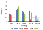
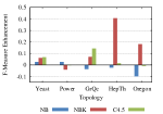
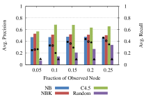
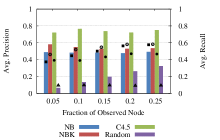
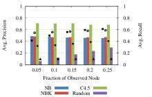
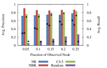
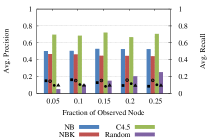
Figure 3(b) shows the F-measure of each classifier using all six features (which includes $P$) minus the F-measure of the same classifiers using feature $P$alone. All classifiers using all features see performance improvements in Yeast compared to their single feature counterparts. In other networks by adding the extra five features the classifiers may, depending on the network, slightly underperform their $P$ feature counterparts, e.g., NB with only $P$ outperforms NB with $P$ and the extra five features in GrQc, HepTh, and Oregon. We conjecture that by adding more features (thus increasing the problem dimension) we make learning more difficulty, resulting in the observed performance degradation. For C4.5 using all six features enhances performance in Yeast and GrQc while there is no significant change over other networks. We note then that for C4.5 feature $P$ is by far the most important feature as adding extra five features in most cases does little to increase the classification accuracy. Note that except for Power, NBK with all features always yields better performance than NBK with feature $P$ alone: in particular, using all features increases the F-measure of NBK applied to in HepTh and Oregon by around 0.4 and 0.2, respectively. Even in Power, the performance degradation of NBK by using all features is not noteworthy. It shows that we can improve the performance of a particular classifier by combining the infection betweenness feature $P$ with the other node features. In future work we will explore other classifiers such as classifiers based on random forests.

4.3.2 Prediction v.s. fraction of observed nodes

In this section, we study the impact of the fraction of observed nodes on the accuracy of our classifiers with all six features. Figure 4 compares the average precision and recall of each classifier according to the fraction of observed nodes. Again, the epidemic infects $10\%$ of nodes. Here, we also compare our classifiers against random-guessing (Random), which tosses a biased coin and with probability 0.1 (0.1 is the fraction of infected nodes) declares the node to be infected. As shown in Figure 4, our classifiers outperform random-guessing both in precision and recall. Also, the precision and recall of our classifiers increases with the fraction of observed nodes; as expected, increasing the fraction of observed nodes provides more information about the infection state of the unobserved nodes.

In a closer look C4.5 exhibits the best precision over all classifiers on almost of all the networks: the only exception is Power, where NBK yields slightly better precision performance than C4.5. Comparing the precisions of each network, we observe that our classifiers show the best precision in Power followed by GrQc, HepTh, Yeast, and Oregon. The power network is almost planar, likely making the classification task easier. In next section, we also explore which network characteristic affects on the performance of our classifiers.

We now look at the recall of each classifier. Figure 4 shows that NBK yields the best recall performance over all the networks except for Power. Note that the precisions of NBK is lower than that of C4.5 except for Power. It means that NBK are more likely to find unknown infected nodes, but its classifications to the infected state are not as accurate as C4.5. When considering each network, all classifiers yield better recall performance in Power. Also, Oregon remains the most difficult network to correctly classify the infected nodes. Even though all classifiers yield relatively high precisions (greater than 0.5) in Oregon, their recall performance in Oregon is less than 0.2, which is similar to that of random-guessing. It means that in Oregon our classifiers make correct decisions when they classify unknown states to infected, but many infected nodes are classified as healthy. In future work, we will explore a method to improve the recall performance of these classifiers using the estimated infected probability.

4.3.3 Impact of Network Characteristics

We now investigate the impact of network characteristics on the performance of our classifiers (using all six features as before). To this end, we investigate the average correlation coefficient between the F-measure performance ranks and ranks of network characteristics for each network; for instance, Oregon has the highest Degree Skewness and NBK is the worst performer among the five classifiers: then we correlate 1 (highest rank in degree skewness) and 5 (worst classifier of five classifiers). Table 2 presents the average Pearson’s correlation coefficient [13] between the ranks of network characteristics and F-measures.

Table 2: Correlation Coefficient between Ranks according to F-measure and Network Characteristics

Characteristic	Correlation
	NB	NBK & C4.5
Clustering Coefficient	0.1	0.2
Standard Deviation of Degree	-0.7	-0.6
Degree Skewness	-1.0	-0.9

As shown in Table 2, the performance of the classifiers is strongly negatively correlated with degree skewness and the degree standard deviation. As the degree skewness and the degree standard deviation decrease the classifiers become more accurate. Interestingly, there is a little correlation between clustering coefficient and classification performance even though an epidemic is more likely to propagate to nodes in a same cluster. A validation with extensive experiment using more networks is part of our future work.

5 Related work

Several methods to detect the presence of network worms and rumor spreading nodes have been proposed in the literature. However, there has been little rigorous work done on inferring the infection state from incomplete data obtained at a relatively few observed nodes without the aid of infection timestamps.

Shah and Zaman [10] studied the problem of finding the source of a computer virus in a network. They focused on how to find the source among the set of infected nodes that are observed, which is different from our goal. Based on their metric called rumor centrality, they constructed a machine-learning estimator that finds the source exactly or within a few hops in networks. They also analyzed the asymptotic behavior of their virus source estimator for regular trees and geometric trees.

Sadikov et al. [9] present an estimation method of network properties, such as the number of weakly connected components, given a sampled network. By formulating a simple $k$-tree model and approximating it to the original network, their method can estimate the properties of original networks; they showed that their method can accurately estimate properties of the original network even when $90\%$ of nodes are not sampled. Zou et al. [15] developed an early detection system to check the presence of a worm in the Internet. The proposed detection approach monitors traffic data at ingress/egree point of a local network. Even with the biased monitored data, it can accurately predict the overall vulnerable population size and estimate how many hosts are really infected in the global Internet system.

Closely related to our work is that of Gomez et al. [1], who develop an algorithm for inferring the network over which a diffusion propagates. Given the observed times when nodes become infected, they determine paths through which the diffusion most likely took, i.e., a directed graph where a contagion passed through. In contrast, our work tries to identify the infection state of each unobserved nodes given a limited number of nodes with known infection state and no infection timestamps.

Jaikaeo et al. [3] presented a malicious node detection method based on comparisons between neighboring nodes, performed on a central server. It is not applicable without a central server which can directly access and inspect each node; thus, their method depends on being able to inspect each node individually.

6 Conclusion

In this paper we studied how to identify the infected nodes without individually inspecting all nodes in the network. Based on the well known SI model, we defined the Infection Betweenness (IB) metric for identifying the latent infection status of nodes. Our empirical results show that the machine learning classifiers with the $I\!B$ metric as feature along with other network-wide features outperform random-guessing and the same classifiers without the $I\!B$ metric as a feature. We also analyzed the impact of the amount of missing data as well as the impact of network characteristics on the effectiveness of the algorithms.

Future work consists of performing more extensive experiments with larger networks, as well as a theoretical analysis about the relationship between network characteristics and performance of the algorithms.

References

- [1] M. Gomez Rodriguez, J. Leskovec, and A. Krause. Inferring networks of diffusion and influence. ACM KDD ’10.
- [2] M. Hall, E. Frank, G. Holmes, B. Pfahringer, P. Reutemann, and I. H. Witten. The weka data mining software: an update. SIGKDD Explor. Newsl., 11(1):10–18, Nov. 2009.
- [3] C. Jaikaeo, C. Srisathapornphat, and C.-C. Shen. Diagnosis of sensor networks. In ICC, volume 5, pages 1627 –1632 vol.5, 2001.
- [4] H. Jeong, S. P. Mason, A. L. Barabási, and Z. N. Oltvai. Lethality and centrality in protein networks. Nature, 411(6833):41–42, May 2001.
- [5] J. Leskovec, J. Kleinberg, and C. Faloutsos. Graphs over time: densification laws, shrinking diameters and possible explanations. ACM KDD ’05.
- [6] J. Leskovec, J. Kleinberg, and C. Faloutsos. Graph evolution: Densification and shrinking diameters. ACM Trans. Knowl. Discov. Data, 1, March 2007.
- [7] M. Newman. Networks: An Introduction. Oxford University Press, Inc., New York, NY, USA, 2010.
- [8] J. R. Quinlan. Improved use of continuous attributes in c4.5. Journal of Artificial Intelligence Research, 4:77–90, 1996.
- [9] E. Sadikov, M. Medina, J. Leskovec, and H. Garcia-Molina. Correcting for missing data in information cascades. ACM WSDM’11.
- [10] D. Shah and T. Zaman. Detecting sources of computer viruses in networks: theory and experiment. ACM SIGMETRICS’10.
- [11] D. J. Watts and S. H. Strogatz. Collective dynamics of ’small-world’ networks. Nature, 393(6684):440–442, June 1998.
- [12] Wikipedia. Skewness — Wikipedia, the free encyclopedia. [Online; accessed 13-Jan-2014].
- [13] Wikipedia. Spearman’s rank correlation coefficient — Wikipedia, the free encyclopedia. [Online; accessed 13-Jan-2014].
- [14] I. H. Witten and E. Frank. Data Mining: Practical Machine Learning Tools and Techniques (Second Edition). Morgan Kaufmann, June 2005.
- [15] C. Zou, W. Gong, D. Towsley, and L. Gao. The monitoring and early detection of internet worms. IEEE/ACM Transactions on Networking, 13(5):961 – 974, oct. 2005.