X-ray spectral modelling of the AGN obscuring region in the CDFS: Bayesian model selection and catalogue
Abstract
Aims. Active Galactic Nuclei are known to have complex X-ray spectra that depend on both the properties of the accreting supermassive black hole (e.g. mass, accretion rate) and the distribution of obscuring material in its vicinity (i.e. the “torus”). Often however, simple and even unphysical models are adopted to represent the X-ray spectra of AGN, which do not capture the complexity and diversity of the observations. In the case of blank field surveys in particular, this should have an impact on e.g. the determination of the AGN luminosity function, the inferred accretion history of the Universe and also on our understanding of the relation between AGN and their host galaxies.
Methods. We develop a Bayesian framework for model comparison and parameter estimation of X-ray spectra. We take into account uncertainties associated with both the Poisson nature of X-ray data and the determination of source redshift using photometric methods. We also demonstrate how Bayesian model comparison can be used to select among ten different physically motivated X-ray spectral models the one that provides a better representation of the observations. This methodology is applied to X-ray AGN in the 4 Ms Chandra Deep Field South.
Results. For the AGN in that field, our analysis identifies four components needed to represent the diversity of the observed X-ray spectra: (1) an intrinsic power law, (2) a cold obscurer which reprocesses the radiation due to photo-electric absorption, Compton scattering and Fe-K fluorescence, (3) an unabsorbed power law associated with Thomson scattering off ionised clouds, and (4) Compton reflection, most noticeable from a stronger-than-expected Fe-K line. Simpler models, such as a photo-electrically absorbed power law with a Thomson scattering component, are ruled out with decisive evidence (). We also find that ignoring the Thomson scattering component results in underestimation of the inferred column density, , of the obscurer. Regarding the geometry of the obscurer, there is strong evidence against both a completely closed (e.g. sphere), or entirely open (e.g. blob of material along the line of sight), toroidal geometry in favour of an intermediate case.
Conclusions. Despite the use of low-count spectra, our methodology is able to draw strong inferences on the geometry of the torus. Simpler models are ruled out in favour of a geometrically extended structure with significant Compton scattering. We confirm the presence of a soft component, possibly associated with Thomson scattering off ionised clouds in the opening angle of the torus. The additional Compton reflection required by data over that predicted by toroidal geometry models, may be a sign of a density gradient in the torus or reflection off the accretion disk. Finally, we release a catalogue of AGN in the CDFS with estimated parameters such as the accretion luminosity in the band and the column density, , of the obscurer.
1 Introduction
Active Galactic Nuclei (AGN) are thought to represent accretion events onto super-massive black holes (SMBHs) at the centres of galaxies. The demographics of this population therefore provide important insights into the formation history of the black holes we observe in nearly all massive bulges in the nearby Universe (Richstone et al. 1998; Shankar et al. 2009). Moreover an increasing body of observational evidence (e.g. Kormendy & Ho 2013, and references therein) as well as theoretical calculations (e.g. Silk & Rees 1998; Fabian 1999; King 2005, 2010) suggest that AGN are also important for understanding the formation and evolution of galaxies. The evidence above motivated efforts to constrain the cosmological evolution of AGN (e.g. Aird et al. 2010) and determine the statistical properties of their host galaxies (e.g. Alexander & Hickox 2012). Despite significant progress in these fields in the last decade important details are still missing. There are for example, open questions relating to the contribution of obscured accretion to the black hole mass budget (e.g. Shankar et al. 2004; Akylas et al. 2012) as well as the overall impact of the energy released by AGN on their immediate environment on kpc and Mpc scales (Kormendy & Ho 2013).
One approach for addressing the points above is via studies of the population properties of AGN averaged over cosmological volumes. The first step in this direction is the characterisation of the basic properties of individual AGN in a statistical sample, e.g. their accretion luminosities, level of line-of-sight obscuration and if possible the basic geometrical properties of the obscuring material in the vicinity of the SMBH. The importance of X-ray observations for constraining these properties are twofold. Firstly, selection at high energies yields AGN samples that are least biased in terms of either line-of-sight obscuration or dilution by stellar light from the host galaxy (Comastri et al. 2002; Severgnini et al. 2003; Mushotzky 2004; Georgantopoulos & Georgakakis 2005). Secondly, because the X-ray flux emitted by AGN is believed to originate at small scales close to the SMBH, spectroscopy at high energies is a unique diagnostic of the accretion properties and the geometry of the material in the vicinity of the central engine.
In this paper we develop a novel framework based on the Bayesian inference to analyse the X-ray spectra of AGN. This method is applied to the problem of the characterisation of the X-ray spectral properties of AGN detected in blank field surveys. Such datasets are extensively used to constrain the statistical properties of AGN and their hosts at moderate and high redshift (), when the bulk of the SMBH we observe in local spheroids were put in place. This particular application is challenging because (i) typical deep field X-ray sources only have a small number of photon counts, well into the Poisson regime, where the familiar -regression approach is often not applicable, (ii) a large fraction of the deep field X-ray sources have redshifts measured via photometric methods (e.g. Salvato et al. 2009, 2011) and therefore suffer uncertainties that affect the inferred X-ray spectral parameters, (iii) it is often difficult for traditional spectral fitting methods to select among different physically plausible spectral models the one that provides a better representation of the observations. A direct result of the latter point is that deep field X-ray spectra are typically fit with simple models (but see for example Brightman & Ueda 2012), because it is unclear whether more complex, but also more realistic, model families are justified by the observations.
The methodology presented in this paper overcomes the issues above by propagating into the analysis and the parameter estimation all the uncertainties related to both Poisson noise and redshift measurement errors. Bayesian model comparison and selection is also used to infer from deep survey observations structural information on the distribution of material close to the SMBH both for individual sources and for the overall population. The field of choice for the application of this methodology is the 4 Ms Chandra Deep Field South (CDFS). This is motivated by the X-ray depth and the availability of multi-wavelength data in that field.
We begin in Section 2 by reviewing our current understanding of the structure of AGN and the physical processes relevant to X-ray emission in the band. In Section 3, the modelling of the spectral components is defined in detail. Section 4 describes the data used. Section 5 presents our approach for comparing models and estimating model parameters. Finally, the results are presented in Section 6 and discussed in Section 7.
2 Spectral components
This section describes the main spectral compoments identified by both observational data and theoretical work which constitute the X-ray spectrum of AGN, although not all of them may be present simultaneously in each source.
X-ray observations show that all AGN share an intrinsic power law spectrum of the form with photon index and a steep cut-off at higher energies (Zdziarski et al. 2000). Observed values for the photon index range between and , and its distribution in local AGN can be approximated by a Gaussian of mean and standard deviation . (Nandra & Pounds 1994). This spectrum is thought to be the result of thermal comptonisation of accretion disk UV radiation by a hot electron corona (Zdziarski et al. 2000; Sunyaev & Titarchuk 1980). A hotter plasma can up-scatter photons to higher energies, thereby producing a power law with a lower photon index. Up-scattering cools the corona which needs to be repopulated with high-velocity electrons to stay in equilibrium. The ultimate source of power is accretion onto the black hole, and thus is thought to be related to physical AGN properties such as the Eddington rate (see Brightman et al. 2013, for a recent discussion).
The intrinsic power law is often obscured by cold material in the line of sight (see e.g. Turner et al. 1997; Risaliti et al. 1999; Brightman & Nandra 2011). The most important effects of this obscuring screen for X-rays are photo-electric absorption, Compton scattering and Fe K-shell fluorescence. Under the unification scheme of AGN (Antonucci 1982; Antonucci & Miller 1985; Antonucci 1993), which postulates that the viewing angle is the main cause for the variety of AGN spectra, the simplest common obscuring geometry is a toroidal structure usually referred to as “the torus”. X-ray observations do not resolve AGN and spectral models can not distinguish the scales at which e.g. photo-electric absorption occurs. However, because the circum-nuclear obscuring material is cold and molecular, it must be distant or self-shielding (see e.g. Gaskell et al. 2008). This picture is further motivated by high-resolution optical space-based observations (Ferrarese et al. 1996; van der Marel & van den Bosch 1998), which show such a torus-like structures in scale, or more recently, mid-infrared interferometry (Burtscher et al. 2013).
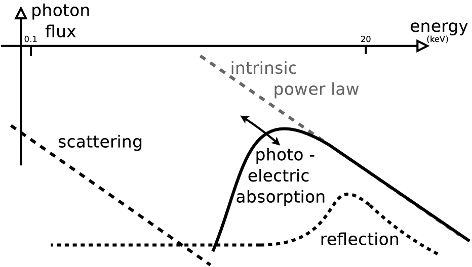
In addition to photo-electric absorption, the obscuring material in the vicinity of the SMBH can also Compton-scatter photons in or out of the line of sight (LOS). Compton scattering, unlike photo-electric absorption, is anisotropic. From a single, unresolved viewpoint, the geometry of the obscurer thus influences the obscured spectrum. For example, compared to a sphere, a torus geometry with a certain opening angle produces a smaller Compton reflection hump between (see Figure 1) , proportional to the solid angle illuminated by the source and the surface area exposed to the observer (Murphy & Yaqoob 2009; Brightman & Nandra 2011). At neutral hydrogen equivalent column densities Compton scattering becomes important compared to photo-electric absorption (Compton-regime).
In obscured AGN, it is believed that a fraction of the intrinsic radiation leaks through encountering no Compton scattering or photo-electric absorption (Ueda et al. 2007). Explanations for this component include Thomson scattering off ionised material within the torus opening angle, which reflects the intrinsic spectrum into the line of sight (Krolik & Kallman 1987; Turner et al. 1997; Guainazzi & Bianchi 2007). This component is referred to as “scattering” in this work, as opposed to “Compton scattering” or “reflection” in the cold obscurer.
In unobscured AGN, extrapolating the power law to softer energies shows an excess of soft X-rays in some sources (Turner & Pounds 1989; Gondhalekar et al. 1997). Processes that have been proposed to explain the soft component include thermal disk emission by the torus at (Gierliński & Done 2004), or a relativistically blurred, photo-ionized reflection spectrum by the accretion disk (Ross & Fabian 1993). In medium-to-high redshift objects, which constitute the bulk of the objects of interest in this work, the soft excess component lies outside the observed energy range and thus we choose to neglect it.
3 Model definitions
The focus of this work is a study of the AGN population to constrain the geometry of the X-ray obscuring material in the vicinity of SMBHs. To identify which physical mechanisms and geometries produce the observed spectra we identify and compare 10 physically motivated models with different levels of complexity. For the model comparison, we develop a Bayesian methodology (discussed in Section 5) that propagates the uncertainties from X-ray observations and redshifts correctly. The data and extraction method is described in Section 4. The spectral components considered are defined below.
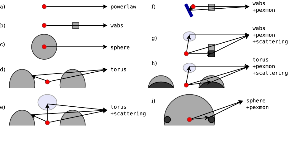
The simplest model considered is a power law, referred to as powerlaw. It represents the intrinsic spectrum of AGN without any obscurer, as shown in Figure 2a). The high-energy cutoff observed in the energy range (Perola et al. 2002) lies well above the energy range used in this work () even at moderate redshifts. We therefore neglect the cutoff. The parameters of powerlaw are the normalisation at and the power law index, .
The most commonly used model to describe obscuration is to apply photo-electric absorption to the intrinsic power law. Absorption has the largest cross-section among the interaction processes, and thus is a good first order approximation for the X-ray spectra of AGN detected in deep fields. However, at higher column densities (), matter becomes optically thick to Compton scattering, and re-emission in lines due to X-ray fluorescence is prevalent. In contrast to photo-electric absorption, which is opaque at low energies, Compton scattering introduces an energy loss at each interaction, thus low-energy photons can be received by the observer. Furthermore, Compton scattering induces a non-uniform scattering angle distribution making the spectrum dependent on the assumed geometry. Influenced by the solid angle illuminated by the source and the surface area exposed to the observer, the contribution by Compton scattering varies, as radiation is scattered into the line of sight. For instance, a torus geometry with a certain opening angle produces a smaller Compton reflection hump between (see Figure 1) than a completely closed, spherical geometry (Murphy & Yaqoob 2009; Brightman & Nandra 2011). The opening angle of the torus, and the viewing angle to a minor degree, thus influences the strength of the reflection hump. This allows in principle to determine the viewing/opening angle and independently, possibly probing the density gradient of the obscurer. However, because the effects on the spectrum are small, particularly in the case of low photon count spectra, this has not yet been successfully applied to discriminate these parameters in individual obscured sources. In this work, we also assume a limited range of geometries (e.g. opening angle, edge-on view) as we do not attempt to constrain the viewing and opening angle. This geometry-dependence of spectra also makes modelling challenging. Multiple inter-dependent interactions of several elements can realistically only be done by X-ray radiative transfer simulations for a fixed geometry (see e.g. Nandra & George 1994; Murphy & Yaqoob 2009; Brightman & Nandra 2011).
In this work, three obscuration models are considered, wabs, sphere and torus, which correspond to different geometries:
The “wabs” model applies only photo-electric absorption on a power law with the cross-sections and polynomial approximations computed by Morrison & McCammon (1983). This model does not include any Compton scattering. It can be considered as an infinitely small blob (see Figure 2b) in the line of sight (LOS): No radiation is scattered into the LOS, and all Compton scattering leaves the LOS. However, the loss of high-energy photons due to Compton scattering at high column densities is not modelled.
We also consider an absorber with spherical geometry (sphere) illustrated in Figure 2c. This model, computed by Brightman & Nandra (2011), consistently models photoelectric absorption, Compton scattering and K-shell fluorescence of a power-law spectrum source at the centre of a cold, neutral medium. Similarly, a toroidal geometry (torus) is used, which was simulated in the same way as sphere, but with a bi-conical cut-out. We restrain the torus model, using a opening angle viewed edge on. The physical scenario represented by this model is shown in Figure 2d, which indicates that Compton scattering into the LOS is possible.
The three obscuration models used mark the extreme cases of torus geometries: wabs for a almost half-opening angle, sphere for a vanishing opening angle and torus represents an intermediate case where 30% of the incident radiation encounters the obscurer. Figure 2b-d illustrates these differences. In comparison to the powerlaw model, wabs, sphere and torus have the additional parameter , the neutral hydrogen equivalent column density in the LOS.
Observations of some obscured AGN show that a fraction of the intrinsic radiation escapes without encountering any obscuration. This is understood to be Thomson scattering off ionised material inside the opening of the obscurer, as illustrated in Figure 2e for the torus geometry. We model this component, referred to as scattering (+scattering) by adding a simple, unabsorbed power law component with the same as the incident radiation. The normalisation of this component, , is modelled relative to the intrinsic power-law component, and may vary between and . In this fashion, torus and wabs are extended to torus+scattering and wabs+scattering. For the sphere model, it should be noted that no unabsorbed radiation can escape, and thus adding scattering is unphysical. However, for completeness, we also consider sphere+scattering, which mimics the case of a torus with a very large covering fraction.
The observed distribution requires a stronger gradient than a constant-density torus geometry can provide (see e.g. Treister et al. 2004). We thus consider an additional density gradient contribution by adding a denser slab outside the LOS inside the obscurer. The – measured largely through photo-electric absorption – indicates only the “effective” column density along the LOS, and thus remains unaffected. However, a denser region outside the LOS can scatter Compton reflection into the LOS, as illustrated in Figure 2g-i. Alternatively, reflection off the accretion disk may also be part of the LOS spectrum entering the obscurer (Fabian 1989; George & Fabian 1991). This is illustrated in Figure 2f for wabs. We thus add a Compton reflection component +pexmon to the obscured spectrum. We assume that this component passes through the obscuring column, so it is introduced photon-absorbed with the same column density as the LOS obscuring material. The used model, PEXMON (Nandra et al. 2007) combines Compton reflection off a neutral dense semi-infinite slab geometry (PEXRAV, Magdziarz & Zdziarski 1995) consistently with , and emission lines and the Compton shoulder (George & Fabian 1991; Matt 2002). We use the same incident spectrum (photon index and no cutoff) for the reflection, and follow Nandra et al. (2007) in assuming a fixed inclination of . The normalisation of this component is modelled relative to the wabs component ( parameter), and may vary between and . Figure 2 illustrates various causes for an additional reflection spectrum (f-i). In the case of wabs model in particular, the +pexmon component can compensate for the lack of forward-scattering inside the obscurer.
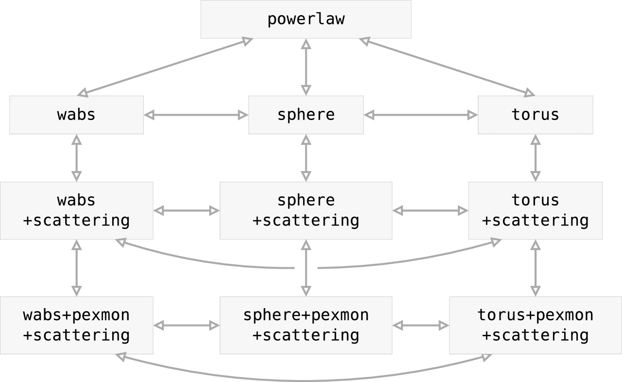
The three obscurer models, wabs, sphere and torus, are compared against each other, as well as the introduction of additional features (+scattering, +pexmon). See text for details.
To summarise, we consider 10 models identified by typewriter font style. The statistical method used for model comparison is described in Section 5. Figure 3 illustrates the comparisons we are interested in with arrows. Firstly, obscurer geometries are compared (powerlaw: no obscurer, Figure 2a; wabs: bullet-like blob, 2b; sphere: complete covering of the source, 2c; torus: intermediate case, 2d). We test for the existence of a soft scattering component which is represented by wabs+scattering, sphere+scattering and torus+scattering (Figure 2e). Finally, we explore the need for additional Compton reflection as shown in Figure 2 f,g for wabs+pexmon+scattering, 2i for sphere+pexmon+scattering and 2h for torus+pexmon+scattering. The following section describes the data to which we apply our methodology.
4 Observational Data
We intend to study the obscuring material in the vicinity of active SMBHs by analysing X-ray spectra with a variety of physically motivated models. The typical SMBH grows through active accretion at redshift (see e.g. Aird et al. 2010). To obtain a sample of such high-redshift AGN, long exposure times are needed. The deepest X-ray survey to date is the Chandra Deep Field South (CDFS) campaign. This survey region has been observed extensively providing excellent multi-wavelength coverage, which we utilise for redshift estimation.
The CDFS survey consists of 51 observations giving a total exposure time of on an area of . Data reduction and source detection followed Laird et al. (2009) and is described in detail in Rangel et al. (2013b, a). Briefly, hot pixels, cosmic ray afterglows and times of anomalously high backgrounds were removed to produce clean level-2 event files. These were then aligned using bright sources and subsequently merged. Images and exposure maps in four energy bands (, , and ) were computed. A candidate source list was created using wavdetect with a low significance threshold (). Source and background counts were extracted on the found positions using the Chandra point spread function tables of Laird et al. (2009). The source region is constructed to contain encircled energy fraction (EEF) of the point spread function (PSF). The background region is a surrounding annulus between EEF PSF and an additional 100 pixel radius. Other candidate sources are masked from the background extraction region. For each candidate source position, the Poisson probability that the observed counts are a background fluctuation was computed, and the source accepted if the significance exceeds (Nandra et al. 2005). This yields a final catalogue of 569 sources.
The ACIS EXTRACT (AE) software package (Broos et al. 2010) was used to extract spectra for each source following Brightman & Ueda (2012). Initially, each source and each pointing is dealt with separately. AE simulates the PSFs at each source position. Regions enclosing PSF at 1.5keV were used to extract source spectra. The background regions are constructed around the sources such that they contain at least 100 counts, with other sources masked out. AE also constructs local response matrix files (RMF) and auxiliary matrix files (ARF) using ray-tracing. As a final step, AE merges the extracted spectra so that each source has a single source spectrum, a single local background spectrum, ARF and RMF. It was possible to extract 567 spectra.
For consistent analysis using Poisson statistics, a model has to be compared to the observed counts. The background contribution can not be subtracted away because unlike in Gaussian distributions, the subtraction of two Poisson distributions does not yield a analytic distribution. It is common practise to use per-bin background estimates. However, this yields unstable results in bins with few counts. We thus choose to model the background in a parametric way using a Gaussian mixture model (see Appendix A for details). This may not be physical but provides a good approximation to the background which is very similar to the On-orbit background measurements in Baganoff (1999) (compare the left panel of Figure 2 therein with Figure 13 in the Appendix). In particular we model a number of instrumental emission lines by introducing Gaussians at mean energies of 1.486 (), 1.739 (), 2.142 (), 7.478 (), 9.713 (; all in keV, Thompson et al. 2001). We allow the centres of these lines to vary within . A feature at (possibly / lines) is described by three additional Gaussians, while the overall continuum shape is modelled of using a flat continuum level and two Gaussians at softer energies (see Appendix A for details). All background model parameters (means, widths, heights) are then fitted to the background spectrum of each source. The goodness of the fit is evaluated using Q–Q plots (see Appendix A for details). The found parameters then remained fixed for the subsequent X-ray spectral analysis of the source spectrum. In general, there may be cases where simultaneous analysis of background and source model parameters provides better results. However, because the larger background region captures many more background photons than the source region, the background model is well constrained by the background data alone.
X-ray spectra extracted from survey data have to be associated with multi-wavelength data to obtain a measure of the distance of each source, i.e. redshifts. For identification of counterparts, the J/K/H-band positions from the CANDELS (Koekemoer et al. 2011; Grogin et al. 2012) CDFS field (Guo et al. 2013; Hsieh et al. 2012) are used in combination with mid-infrared positions from IRAC (Damen et al. 2011; Ashby et al. 2013). A Bayesian method was developed that matches X-ray positions to mid- and near-infrared counterparts simultaneously (Budavári & Szalay 2008, Salvato et al. in prep). For 528 sources optical counterparts have been found (see Hsu et al., in prep). For 301 sources, reliable spectroscopic redshifts are available (Hathi et al. in prep); for 185 of the remaining sources, photometric redshifts were successfully computed, giving a total of 476 sources.
Optical, IR and UV photometry was used from the TFIT 10-epoch multi-wavelength catalogue (Guo et al. 2013) within the CANDELS GOODS South Survey, 32-band data from the MUSYC survey (Cardamone et al. 2010) and Far/Near-UV from GALEX. Outside the CANDELS region, TENIS J/K band data (Hsieh et al. 2012) was used. The computation of photometric redshift by Hsu et al. (in prep) follows the same SED fitting procedures described in Salvato et al. (2011), using SED templates from Ilbert et al. (2009) and Salvato et al. (2009) and software developed for Arnouts et al. (1999) and Ilbert et al. (2006).
While it is common practise to merely use the best fit redshifts, here we marginalise the probabilities to obtain photometric redshift probability distributions (“photo-z PDFs”). The benefit is that all solutions are considered in subsequent analysis. The benefits of propagating the uncertainty of the redshift determination is demonstrated in Appendix B, by comparing to using a point-estimator. By an instructive example, it is demonstrated there that Maximum Likelihood fitting methods can significantly underestimate the uncertainty in the derived parameters. A future improvement could be to incorporate systematic errors into these PDFs.
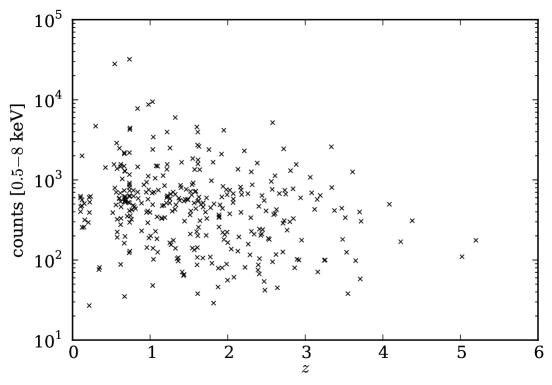
Star-burst galaxies can contaminate the sample and skew the inferences we try to make about AGN, especially with regards to the soft energy ranges. We adopt the criteria for inclusion of AGN from Xue et al. (2011): Sources with , effective power law index and are not used. The criterion selects weak X-ray sources that are much brighter in the optical, and additionally emit mostly soft X-rays. This selection is designed to exclude sources with non-negligable host contribution. Thus, AGNs in star-burst galaxies and low-luminosity AGN are not studied. Furthermore, objects classified as stars or galaxies (i.e. host-dominated sources in the X-ray) by Xue et al. (2011) are removed. 346 AGN remain.
Model selection assumes that one model is the correct one (see Section 5.3 below). For determining whether the model could produce the data at hand, we adaptively bin the spectrum counts so each bin contains 10 counts. Then we compute the -Statistic for the best fit model parameters. If , where is the number of bins, the object is not used for model comparison. For low count spectrum, this criterion is relaxed further (2.3 if less than 500 counts, 3 if less than 100 counts, 5 if less than 50 counts) due to the stronger Poisson variance. These limits were obtained by simulating a flat Poisson spectrum across bins, so that they exclude the true value in fewer than 1% of the simulations. The 13 affected sources were visually inspected in the X-ray and optical and at least 5 of them can be clearly explained by outliers in the photometric redshift due to contaminated photometry or incorrect association. With an outlier fraction of , the expected number of outliers is . 334 AGN remain.
It is worth noting that in this work the selection criteria are of minor importance, as the unification argument is not applied. Instead of assuming a common torus that is viewed from a variety of angles, we only require that all sources considered are built using (a subset of) the same physical processes.
5 Statistical analysis methods
5.1 Parameter estimation
In X-ray spectral analysis it is common practice to vary the parameters of the spectral components until a certain statistic is optimized with regard to the observed X-ray spectrum.
Because X-ray sources in deep extragalactic surveys are typically faint, their spectral bins are filled by counts according to a Poisson process. A statistic is not applicable. Re-binning the data to use a -statistic is a common practise, however this results in loss of information in the energy resolution. Additionally, the reliability of the -estimator is unknown if the incorrect model () is used, and thus its confidence intervals are problematic.
The maximum likelihood C-statistic (Cash 1979), based on the Poisson likelihood , does not suffer from these issues. However it is not useful as a measure of goodness-of-fit. Both the -statistic and denote the of a likelihood, and the statements made for are also applicable to . While is not -distributed, is, according to Wilks’ theorem (Cash 1979; Wilks 1938).
For optimising the parameters, one can not simply step through the parameter space due to the curse of dimensionality. Typically, local optimisation algorithms like the Levenberg-Marquardt algorithm (Levenberg 1944; Marquardt 1963) are employed to iteratively explore the space from a starting point. The final point is taken as the most likely parameter vector. If there are multiple, separate, adequate solutions, i.e. local probability maxima, in the parameter space, these algorithms can not identify them or jump from one local maximum to the other.
For error estimation, there are three commonly used options: (1) Assume independence of parameters and Gaussian errors, and estimate the error for each parameter in turn by finding the value where the statistic drops by a level corresponding to . (2) assume Gaussian errors, estimate the local derivatives and invert the Fisher matrix, (3) compute contours of some value motivated by the distribution. The last is more computationally costly than optimisation and can at most be done in 2 dimensions at a time. These three error estimates are approximations that are only sufficient in the case where the probability distributions either approach the shape of a single Gaussian, or the interdependency between parameters is negligible. A general maximum likelihood approach that does not have these shortcomings is to estimate the error using simulated data to find a confidence interval () that contains the used parameter e.g. of the time. This is the most costly option, as it fits to generated data many times.
Alternatively, a Bayesian approach can be adopted, e.g. van Dyk et al. (2001) introduces Bayesian X-ray spectral analysis in detail. As before, the Poisson likelihood is used to explore a parameter space. However, there are some important differences. The space is now weighted or deformed by priors. The goal in Bayesian parameter estimation is to identify sub-volumes which constitute the bulk of the probability integral over the parameter space. This approach does optimisation and error estimation simultaneously, but requires an integration and exploration technique that does not suffer from the curse of dimensionality.
Markov Chain Monte Carlo is a commonly employed integration method for Bayesian parameter estimation. This algorithm tests a starting point against a new random point chosen from the prior distribution with a local bias. With a probability proportional to the ratio of the two points, the algorithm picks the new point as the new starting point. With each iteration producing a point, a chain is created with the interesting property that parameter vectors are represented proportional to their probability. This full representation of the parameter space can be marginalized to look separately at each parameters distribution. Furthermore, error propagation in derived quantities can be done correctly without assuming a underlying normal distribution.
MCMC has its own share of problems however. First, convergence, i.e. if a chain has become a proper representation of the parameter space, can not be tested for. Only non-convergence may be detected. For example, a chain can stagnate for a while but at a later point suddenly discover a parameter sub-space of high probability. When or if this would happen however, can not be determined. As a local algorithm, MCMC has great difficulty finding and jumping between well-separated maxima. MCMC is a powerful algorithm also applicable to high dimensionality, and thus many extensions and variants have been developed for MCMC to mitigate these issues.
Our approach for circumventing the problems of MCMC in exploration and integration of parameter spaces is to use a different Monte Carlo algorithm, Nested Sampling (Skilling 2004). Nested Sampling keeps a set of fixed size of parameter vectors (“live points”) sorted by their likelihood. These points are always randomly drawn from the prior distribution. The algorithm then removes the least likely point by drawing points until one is found with a higher likelihood. Effectively, this approach “scans” the parameter space vertically from the least probable zones to the most probable. For each removed point, the volume this point is representative for is computed, and the according probability mass added to the integration. When the remaining parameter volume is negligible, the algorithm terminates. A difficulty of this algorithm is to avoid the curse of dimensionality when drawing from the prior distribution to get higher valued points.
MultiNest (Feroz et al. 2009) solves this problem efficiently by clustering the live points into multi-dimensional ellipses, and drawing from these subspaces under the assumption that higher-valued points can only be found in proximity of already drawn points. Because of the clustering, MultiNest can follow distinct local maxima without difficulty. MultiNest is applicable to the low-dimensional problems of X-ray spectral modeling. It can compute points of equal weighting akin to a Markov Chain, provide values and error estimates for each local maximum as well as marginal probability distributions for each parameter. The integral over the parameter space is computed globally and for each local maximum.
5.2 Model comparison
For classic model comparison, Wilks’ theorem can be used, which states that the difference in the best fit -statistic is -distributed with the degrees of freedom equal to the difference in number of parameters (Wilks 1938). This asymptotic result is only valid for nested models, i.e. M1 is a special case of M2.
Bayesian model comparison is done by comparing the integrals over parameter space, called the evidence , where is the parameter vector and represents the weighting or the deformation of the parameter space by the prior. Often, the logarithm is computed. The Bayes factor is then compared to the a priori expectation. This method does not require models to be nested nor does it make assumptions about the parameter space or the data. Without altering the Bayes factor, the used statistic can be modified by arbitrary constants as long as they are independent of the parameters.
Alternatively, information criteria can be used. These are approximations in the limit using certain assumptions, which compare the difference in the best fit -statistic between the models to an over-fitting penalisation term. Typically, the more complex model is punished by the additional number of parameters. Computation is thus very similar to Wilks’ theorem, although the background is very different.
The Bayesian information criterion (BIC, Schwarz 1978) is an approximation to Bayesian model comparison. Unlike in the Bayesian evidence integration, only the maximum likelihood is needed, as the posterior is assumed to be strongly single-peaked, making the prior negligible. Because the BIC uses the Laplace integral approximation, its results are in principle unreliable at the boundaries of the parameter space (e.g. checking whether a non-negative parameter is zero). The BIC decides, just like Bayesian model selection, which model is more probable to have produced the data. The model with the smallest should be preferred, where is the number of observations (data points) and donates the number of free parameters of the model.
The Akaike Information Criterion (AIC, Akaike 1974) is not rooted in Bayesian inference, but information theory. The AIC measures the information loss by using a specific model. Thus it can be said to consider the case of having multiple data sets and predicting the next. Technically, the Kullback-Leibler divergence, sometimes referred to as the “surprise” or “information gain” is minimised. The model with the smallest should be preferred.
5.3 Model verification
Any model comparison, or more generally any inference problem, assumes that one of the stated hypotheses is the true one. If no model is correct, the least bad model will be preferred. However, this assumption also requires examination.
Traditionally, this is quantitatively addressed by Goodness of Fit (GoF) measures such as the reduced for normal distributions, with posterior-based approaches such as posterior predictive tests recently being developed (see e.g. Bayarri & Castellanos 2008). No consensus has been reached on these methods. Asymptotic results make assumptions not applicable in practice (e.g. the Likelihood-ratio and F-test are invalid at boundaries, making them unsuitable for feature-detection problems, see Protassov et al. 2002). Posterior-based approaches are diverse, and can be overly conservative (see e.g. Sinharay & Stern 2003). In the strict sense, there is no probabilistic framework available, frequentist or Bayesian, for testing whether the fitted model is correct.
We can, however, relax the question to ask whether the model ”explains” the data by looking at the range covered in the observable. Monte Carlo simulations (parametric bootstrap) can be performed with the best-fit parameters to check whether the spectrum can actually be produced by the given model. This can be computationally expensive however. It is easier to use a measure of “distance” between model and data (e.g. the Kolmogorov-Smirnov statistic) to discover potentially problematic cases and to visually examine the data.
Q–Q plots (Wilk & Gnanadesikan 1968, , see Appendix A) provide a generic tool to visualise the goodness of fit, and are independent of the underlying distribution. The quantiles of the integrated observed counts are plotted against the integrated expected counts from the model. A good fit shows a straight line (). This method is shown in Appendix A: The Q–Q plot is used for model discovery for improved fits, while model comparison using the AIC tests the significance of the model alterations.
5.4 Experiment design and predictions
When a result turns out to be inconclusive, it is often interesting to find out whether a future observation can improve the discriminatory power, i.e. how well parameters can be constrained or whether two models can be distinguished. Classically, simulations are employed with a specific setup. A large number of data sets is generated and fitted. The distribution of best fit values then shows the uncertainty.
Alternatively, the Bayesian analysis can be employed. Here we only consider a simple approach, while Bayesian Experimental Design theory – a theory based on maximising the information gain – is not covered. Since the diversity of possible spectra is less interesting than determining the discriminatory power regarding parameters or models, it is sufficient to generate and analyse a single spectrum for each problem as the Poisson likelihood is already informative of the uncertainty. This was done in Georgakakis et al. (2013) for Athena+/WFI predictions to detect and measure outflows. For a grid of problems () the ability to distinguish a warm absorbers from a cold absorber were tested using the same Bayesian spectral analysis methodology laid out here, and the uncertainty of parameters recorded.
5.5 Priors
A model definition in the Bayesian framework would be incomplete without describing the priors to the models defined above. These encode an a priori weighting within the parameter space. Equivalently, a transformation of the unit space to the parameter space is sought. The simplest case is a uniform prior, giving equal weight in the parameter space. However, a uniform prior means something different whether the parameter or its logarithm is used. The parameters are very similar across the models used, so we describe them all together.
In the problem at hand, we assume the prior distributions to be independent. We use log-uniform priors for scale variables such as normalisations and . The normalisation of spectral models is allowed to vary between and . This conservatively contains physically possible photon fluxes. However, since all considered models contain this parameter, the limits are irrelevant in practise. The normalisation of individual spectral components is then modelled relative to this model normalisation. is defined from to . The photon index is modelled after the local sample analysed in Nandra & Pounds (1994), as a normal distribution with mean and a standard deviation of . This encodes the assumption that distant AGNs behave like local AGNs with regard to their intrinsic spectrum. There is a degeneracy between and in that a steeper power law can be flattened by absorption. Hence, placing a prior on plays an important role in constraining . Nevertheless, we found that our results (e.g. the distribution of the analysed sample) are insensitive to other choices (for instance from de Rosa et al. 2012), as the data drive the result in the majority of cases. While redshift and use informed priors, all remaining parameters, unless otherwise stated, are assumed to be location parameters and thus have a uniform prior.
Of course we are not interested in our prior beliefs, but in how the data strengthens or weakens hypotheses and re-weights parameter space. If the data has no discriminatory power, there is no information gain and the prior and posterior probability distributions will look the same. The difference between the prior and posterior can be measured using the Kullback-Leibler divergence (Kullback & Leibler 1951) as , essentially a integral difference across the parameter space. The KL divergence is measured in ban, a unit of information or entropy. A considerable information gain is e.g. which corresponds to halving the standard error of a Gaussian. We will restrict ourselves to computing the information gain only for the parameter.
For model comparison, we furthermore need to specify our a priori preference of models. We consider two approaches: a) pair-wise comparisons from low to high complexity (e.g. torus vs. torus+scattering, see Figure 3), and between models of the same complexity. We adopt the scale of Jeffreys (1961): A Bayes factor above 100 is “decisive”, 30 “very strong evidence”, 10-30 “strong evidence”, 3-10 “substantial evidence”. In , this corresponds to differences of 2, 1.5, 1 and 0.5 respectively. In case of a Bayes factor below 10 we remain with the simpler model. b) comparing all models simultaneously to find the model with the highest evidence. In both cases we consider the models a priori equally probable.
5.5.1 Implementation
For the spectral analysis in the framework of Bayesian analysis, the MultiNest library was used and two software packages were created: PyMultiNest is a generic package for connecting Python probability functions with the MultiNest library, as well as model comparison and parameter estimation analysis of the MultiNest output. BXA is a package that connects the Sherpa X-ray analysis framework (Freeman et al. 2001) with our Bayesian methodology. (Py)MultiNest repeatedly suggests parameters on a unit hypercube which are transformed by BXA into model parameters using the prior definitions. BXA then computes a probability using Sherpas C-stat implementation, which is passed back to (Py)MultiNest. (Py)MultiNest can then be used to compute Bayes factors, create one or two-dimensional marginalised posterior probability distributions (PDFs) and output summarising Gaussian approximations.
BXA and PyMultiNest are publicly available on http://github.com/JohannesBuchner. In this work, MultiNest v2.17 is being used by BXA on Sherpa version 4.4v2 with 400 live points and a log-evidence accuracy of . For further analyses, we made extensive use of the Numpy/Scipy, Matplotlib and Cosmolopy packages (Jones et al. 2001–; Hunter 2007, http://roban.github.com/CosmoloPy/) packages.
6 Results
| Model | BIC | AIC | ||||||
|---|---|---|---|---|---|---|---|---|
| (1) | (2) | (3) | (4) | (5) | (6) | (7) | (8) | |
| torus+pexmon+scattering | 1.43 | 0.0 | 40.0% | -109.40 | -122.59 | |||
| sphere+pexmon+scattering | 1.46 | -0.1 | 30.2% | -109.40 | -122.59 | |||
| wabs+pexmon+scattering | 1.44 | -0.1 | 29.0% | -109.43 | -122.62 | |||
| torus+scattering | 1.42 | -2.0 | 0.4% | -105.18 | -113.97 | |||
| sphere+scattering | 1.45 | -2.1 | 0.3% | -105.87 | -114.67 | |||
| wabs+scattering | 1.44 | -2.7 | 0.1% | -103.08 | -111.88 | |||
| sphere | 1.52 | -4.7 | 0.0% | -98.07 | -102.47 | |||
| torus | 1.54 | -4.7 | 0.0% | -97.63 | -102.02 | |||
| wabs | 1.58 | -5.5 | 0.0% | -95.13 | -99.53 | |||
| powerlaw | -27.9 | 0.0% | 0.00 | 0.00 |
The Bayesian methodology of parameter estimation and model comparison presented in Section 5 is applied using the models introduced in Section 3 to all sample spectra (see Section 4). To demonstrate the methodology, we first discuss a single source. Then we apply model comparison across the full sample.
6.1 Source 179
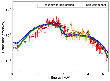
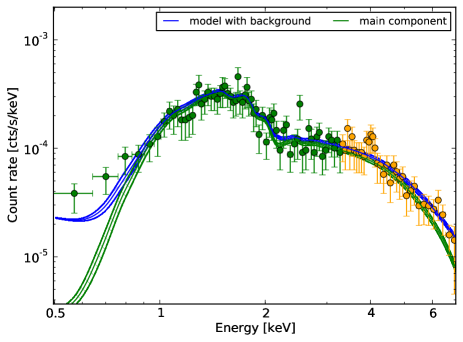
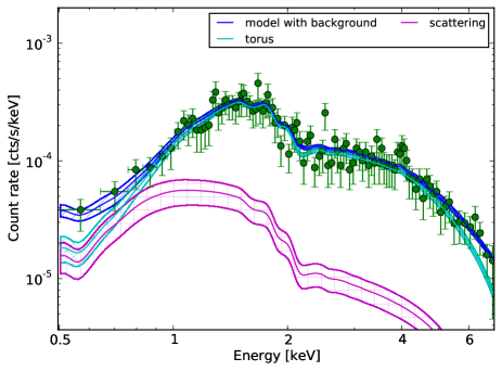
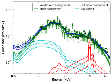
Source 179 (spectroscopic , GOODS-MUSIC 15626) was detected with 2485 counts in the band at RA/Dec=(3:32:13.23, -27:42:41.02). This source was chosen because it illustrates the model selection well, showing several features, namely the Fe-K line, scattering and absorption. In the next few paragraphs we present the source’s spectrum and how well different models reproduce them. Figure 5 overlays different models to the observed data. For brevity, only a subset of models are included in this presentation, namely powerlaw, wabs, torus+scattering and wabs+pexmon+scattering. We then show the results of model-selection for this object in Table 1, where the -column (normalised to highest) shows the computed evidence. Finally, the derived posterior parameters are shown.
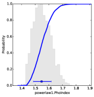
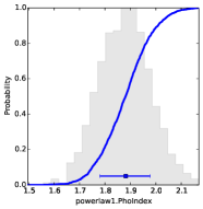
A power law model (powerlaw) does not provide a good fit. This can be seen in the deviations between model and data points in the upper left panel, and also in the fact that this model has the lowest evidence of all models Table 1 (column 5). Furthermore, the derived photon index, is unlikely and would constitute a outlier.
Obscuration is expected in some sources, and the wabs model indeed improves the fit. The model follows the spectrum much closer (upper right panel in Figure 5) with a line-of-sight absorption of . The evidence for this model is significantly higher, and rules out the powerlaw model. Here we consider a difference of as a significant preference (see Section 5.5). The same is true for sphere and torus models not shown here.
Comparing the data with the model prediction in the wabs spectrum, a line is visible at as well as an excess of soft energy counts. The former coincides with the Fe-K line, while we expect to model the latter with the +scattering component. Considering torus+scattering and wabs+pexmon+scattering (lower panels in Figure 5), they both model the observed counts well. However, the Fe-K line is clearly visible in the data. Compared to the simple absorption models, the addition of +scattering and +pexmon increases the evidence (see Table 1), hence these models are preferred, while the other models, e.g. the widely used wabs+scattering, are ruled out for this source.
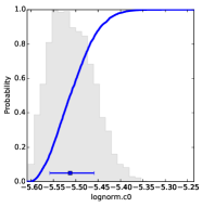
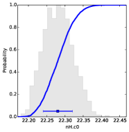
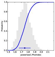
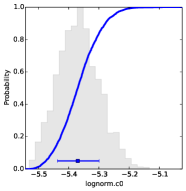
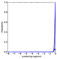
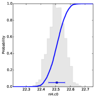
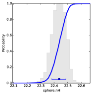
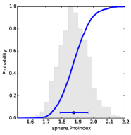
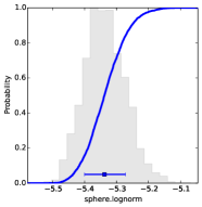
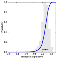
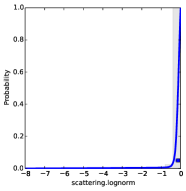
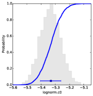
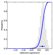
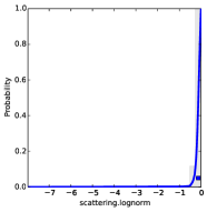
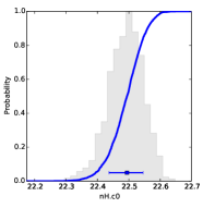
When comparing models, an important aspect is the model-dependence of derived physical parameters. In Table 1, we show the intrinsic luminosity, photon index and line-of-sight column density. These are computed by the posterior values and summarised using -equivalent quantiles. The marginal posterior distributions are shown in Figure 6. Simple absorption model like wabs try to compensate the soft X-rays by using a flatter spectrum with less absorption. Both the +scattering and +pexmon component increase the photon index. As these additional components only take up a fraction of the intrinsic power law component, the changes in intrinsic luminosity are small. Despite these changes, in between obscurer geometries (i.e. wabs, torus, sphere), the values are consistent.
Furthermore, it is important to check whether the results on the derived physical parameters are strongly influenced by the prior. For example, for a weak source with data of no discriminatory power, the posterior of would look like the prior (log-uniform). We use the KL-divergence (see Section 5.5), also known as the information gain or knowledge update, to measures the “distance” between prior and posterior of . For this particular source, the values are shown in column 4 of Table 1. For reference, a considerable information gain is e.g. which corresponds to halving the standard error of a Gaussian. Because is well-constrained in this source compared to the prior, the values are high, and the posterior is not dominated by the prior.
The BIC and AIC values (column 7 and 8 of Table 1, lower values are preferred) show the same preferences as the Bayesian evidence computations. They are an approximate method of model selection based on the likelihood ratio and parameter penalisation. There are however important differences to the Bayesian model selection (see Section 5.2 for details). The evidence and its approximation, the BIC, can be used to express how much more probable a model is compared to the others based on the data (column 6). The AIC, in contrast, measures the information loss by using a specific model. In this single source, the model selection prefers models with absorption, scattering and an additional reflection component (pexmon). However, no preference is found between the geometries of wabs, torus and sphere. To improve the discriminatory power, we combine the evidence of the full sample.
6.2 Model selection on the full sample
We present the results for the full sample in two forms. Firstly, in each source, we perform model comparison between each pair of models (arrows in Figure 3). We count for how many sources a preference was found. This is shown in Figure 7, where the two numbers indicate the two directions. For instance, in 6 sources, the (simpler) powerlaw model is preferred over the torus, while in 170 sources, the torus is preferred. The size of the arrows visualises the same information. There is clear preference for absorption, scattering and reflection in , and cases respectively, showing that in a substantial number of sources these components are required. Between wabs+pexmon+scattering, torus+pexmon+scattering and sphere+pexmon+scattering, there is no clear trend, however the torus geometry is preferred most often. This indicates some variety in the obscurer geometry between sources.
| Sample results | Bootstrapped results | ||||
| Model | # rej | # rej | ruled out | ||
| (1) | (2) | (3) | (4) | (5) | (6) |
| All (334 sources) | |||||
| torus+pexmon+scattering | |||||
| wabs+pexmon+scattering | |||||
| sphere+pexmon+scattering | |||||
| torus+scattering | |||||
| sphere+scattering | |||||
| wabs+scattering | |||||
| torus | |||||
| sphere | |||||
| wabs | |||||
| powerlaw | |||||
| (54 sources) | |||||
| wabs+pexmon+scattering | |||||
| sphere+pexmon+scattering | |||||
| powerlaw | |||||
| (47 sources) | |||||
| torus+pexmon+scattering | |||||
| sphere+pexmon+scattering | |||||
| wabs+pexmon+scattering | |||||
| torus+scattering | |||||
| (51 sources) | |||||
| wabs+pexmon+scattering | |||||
| torus+pexmon+scattering | |||||
| (14 sources) | |||||
| torus+scattering | |||||
| torus+pexmon+scattering | |||||
| torus | |||||
| (176 sources) | |||||
| torus+pexmon+scattering | |||||
| wabs+pexmon+scattering | |||||
| (229 sources) | |||||
| torus+pexmon+scattering | |||||
| wabs+pexmon+scattering | |||||
| torus+scattering | |||||
| (96 sources) | |||||
| torus+pexmon+scattering | |||||
| torus+scattering | |||||
| wabs+pexmon+scattering | |||||
| sphere+scattering | |||||
Secondly, we show the model comparison across all sources in Table 2. For each model, the evidence is stacked in column 3 by summing the values. This form of model comparison assumes that one common model describes all sources. For comparison, column 2 shows the number of sources for which the model was ruled out by the other models. As shown with Source 179 above, individual sources can already have strong preferences in the model selection. To have a result descriptive of the sample that is not dominated by outliers, we apply bootstrapping. Sources are drawn with repetition, and the same quantities (number of rejections, summed values) are computed, and taking all draws together the mean and root mean square is estimated. Additionally, we compute for each draw whether this model is ruled out (). If the model is ruled out in of draws (column 6), the result is robust against bootstrapping and thus there is confidence that this result will also hold for the parent sample and is not dominated by outliers.
The power law model (powerlaw) has the lowest evidence and is ruled out by simple absorption models. These in turn are ruled out by absorption with additional scattering (in Figure 7, strongly preferred in 15-23 objects). Then, for 6-23 objects additional pexmon reflection is strongly preferred.
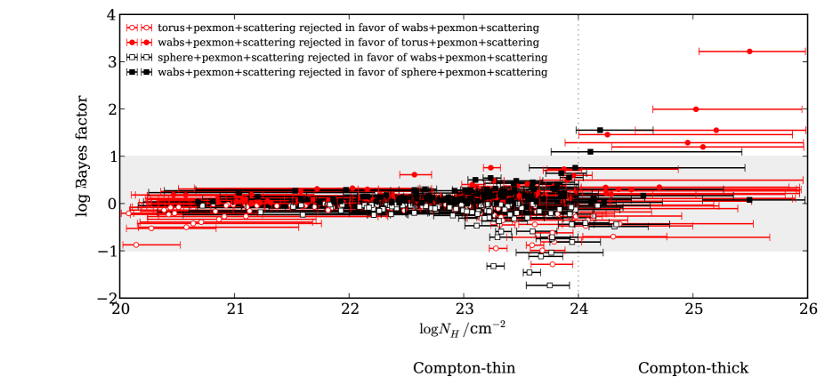
The remaining models are thus such that absorption, scattering and reflection are required. The number of objects for which a model is rejected remains comparable between wabs+pexmon+scattering, sphere+pexmon+scattering and torus+pexmon+scattering, with the latter having the highest evidence. The results for the full sample have significant large differences in . But when bootstrapping the values show large variation and overlap broadly, showing that the difference is not robust against bootstrapping, and sample-dependent. This indicates considerable variation in evidence, i.e. variation in the models preferred, between sources. We investigate this by splitting the samples by (lower segments of Table 2). For this, we assign a source to a bin if the quantiles of the posterior values determined from torus+scattering fall inside. As indicated before, is comparable between absorption models. Figure 9 shows the differences in evidence between the two best models, wabs+pexmon+scattering and torus+pexmon+scattering in blue circles.
In the Compton-thick regime (), torus+pexmon+scattering is consistently strongly preferred. However, both the table and the figure show only mild indication that the torus+pexmon+scattering model is the best across the full sample. Thus some sources must favour wabs+pexmon+scattering, while others favour torus+pexmon+scattering (see Figure 9).
A further concern might be that low-redshift sources with many counts dominate the result, ignoring the target population of our inference. The last two segments of Table 2 shows the result of selecting only sources with and respectively. The inference results in this regime are entirely consistent with the results for the full sample.
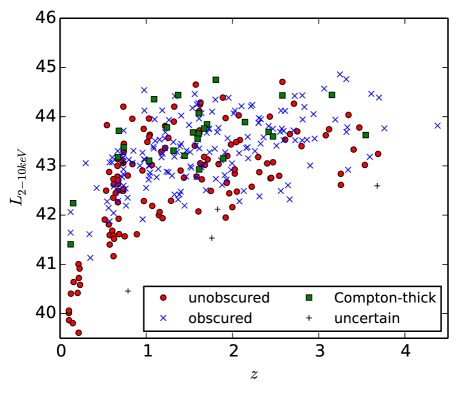
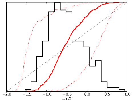
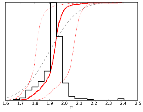
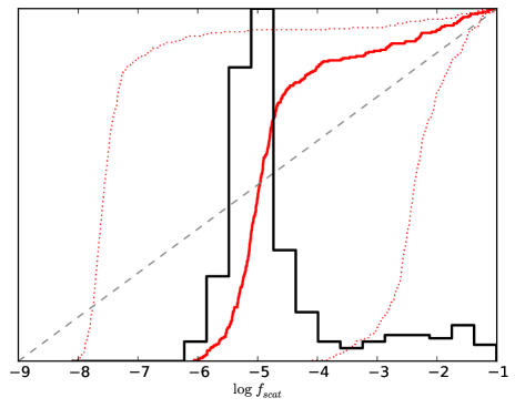
Overall however, torus+pexmon+scattering can be considered the best model. We release a catalogue of the derived quantities for each source in the CDFS (Table 3 shows an excerpt, Table 4 lists all Compton-thick sources; the complete catalogue is available electronically). In particular, we list column densities, intrinsic power law index, intrinsic luminosity as well as the relative normalisations of the additional scattering and reflection components. Full probability distributions are available on request. The most important parameters for e.g. luminosity function studies are , and , which are visualised in Figure 8.
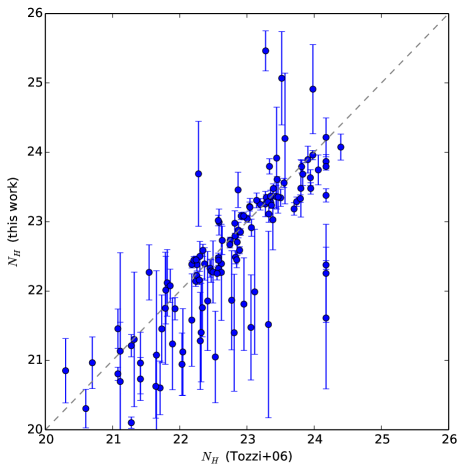
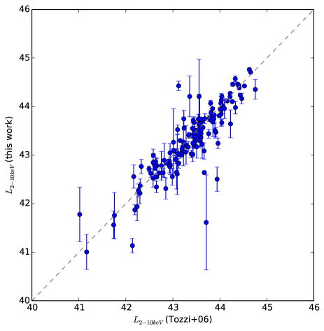
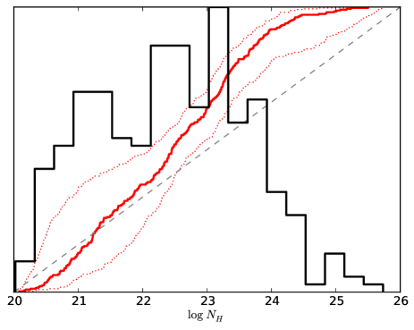
We plot the median and 1-sigma equivalent quantiles of the posterior in our analysis against the best fit found in Tozzi et al. (2006). There are important differences between the works. The Tozzi et al. (2006) analysis is based on only the first 1Ms data, and thus has much fewer counts. Furthermore, only simple absorption models have been considered in their maximum likelihood fitting.
Figure 11 shows a comparison to previously published works in the CDFS. Without going into detail here (see figure caption), the found Compton-thick AGN are in agreement with the sample found by Brightman & Ueda (2012), except that our selection criterion removes a number of sources whose soft photons are dominated by stellar processes. One source (ID 186 in their paper), is not found to be a Compton-thick AGN, as a different redshift from the improved catalogue (Hsu et al., in prep) was used.
| ID | RA | Dec | counts | notes | |||||||
|---|---|---|---|---|---|---|---|---|---|---|---|
| (1) | (2) | (3) | (4) | (5) | (6) | (7) | (8) | (9) | (10) | (11) | (12) |
| 49 | 3:32:14.01 | -27:51:00.53 | 1997 | 0.122 | O,s | ||||||
| 242 | 3:31:52.35 | -27:47:52.79 | 762 | U,R | |||||||
| 21 | 3:32:12.94 | -27:52:36.57 | 957 | 2.562 | O,R | ||||||
| 131 | 3:32:22.54 | -27:46:03.84 | 597 | 1.727 | O,S | ||||||
| 118 | 3:31:52.53 | -27:46:42.30 | 1295 | 0.673 | U,R | ||||||
| 338 | 3:32:49.20 | -27:40:50.01 | 667 | O,s | |||||||
| 144 | 3:32:29.98 | -27:45:29.96 | 3961 | 1.218 | U,R | ||||||
| 104 | 3:32:08.66 | -27:47:34.34 | 28019 | 0.543 | U,R | ||||||
| 190 | 3:32:27.00 | -27:41:05.11 | 32099 | 0.734 | U,R | ||||||
| 92 | 3:31:58.11 | -27:48:33.97 | 915 | 0.734 | U,R | ||||||
| 179 | 3:32:13.23 | -27:42:41.02 | 2485 | 0.605 | O,S,R | ||||||
| 287 | 3:31:55.40 | -27:54:47.21 | 618 | 0.737 | O,s | ||||||
| 4 | 3:32:38.90 | -27:57:00.17 | 4687 | 0.297 | O,s,R | ||||||
| 133 | 3:32:39.08 | -27:46:01.79 | 1355 | 1.216 | O,S | ||||||
| 50 | 3:32:18.34 | -27:50:55.13 | 647 | 1.536 | O,s | ||||||
| 181 | 3:32:47.88 | -27:42:32.78 | 8718 | 0.979 | O,S | ||||||
| 132 | 3:32:03.66 | -27:46:03.74 | 1380 | 0.574 | O,R | ||||||
| 7 | 3:32:40.82 | -27:55:46.76 | 1557 | O,s | |||||||
| 200 | 3:32:34.39 | -27:39:13.55 | 1848 | O,s |
| ID | RA | Dec | counts | notes | |||||||
|---|---|---|---|---|---|---|---|---|---|---|---|
| (1) | (2) | (3) | (4) | (5) | (6) | (7) | (8) | (9) | (10) | (11) | (12) |
| 460 | 3:32:23.41 | -27:42:55.89 | 194 | 2.145 | CT | ||||||
| 420 | 3:32:23.60 | -27:46:01.23 | 48 | 1.033 | CT | ||||||
| 412 | 3:32:42.87 | -27:48:09.44 | 67 | CT | |||||||
| 448 | 3:32:19.41 | -27:40:51.76 | 528 | 0.682 | CT | ||||||
| 474 | 3:32:15.81 | -27:42:06.78 | 339 | CT | |||||||
| 271 | 3:32:33.86 | -27:42:04.30 | 306 | CT | |||||||
| 478 | 3:32:14.60 | -27:52:57.06 | 164 | CT | |||||||
| 467 | 3:32:00.80 | -27:53:33.84 | 541 | CT | |||||||
| 437 | 3:32:39.15 | -27:48:32.26 | 54 | 2.470 | CT | ||||||
| 345 | 3:32:24.67 | -27:54:43.24 | 255 | 0.123 | CT | ||||||
| 451 | 3:32:31.49 | -27:50:28.64 | 38 | 1.613 | CT | ||||||
| 266 | 3:32:14.94 | -27:42:24.83 | 976 | CT | |||||||
| 416 | 3:32:21.77 | -27:46:56.99 | 64 | CT | |||||||
| 406 | 3:31:45.16 | -27:49:48.72 | 571 | 3.153 | CT | ||||||
| 400 | 3:32:25.18 | -27:54:49.72 | 346 | 1.090 | CT | ||||||
| 404 | 3:32:36.15 | -27:50:36.97 | 108 | 1.608 | CT | ||||||
| 401 | 3:31:50.45 | -27:52:11.49 | 592 | 1.370 | CT | ||||||
| 158 | 3:32:22.59 | -27:44:25.97 | 129 | 0.738 | CT | ||||||
| 77 | 3:32:35.71 | -27:49:16.18 | 95 | 2.578 | CT | ||||||
| 417 | 3:32:21.97 | -27:46:56.00 | 35 | 0.670 | CT | ||||||
| 570 | 3:33:00.76 | -27:48:57.46 | 438 | CT | |||||||
| 226 | 3:32:14.42 | -27:51:10.43 | 141 | 1.544 | CT | ||||||
| 441 | 3:32:22.79 | -27:45:28.54 | 46 | CT | |||||||
| 408 | 3:32:33.22 | -27:49:15.92 | 38 | CT | |||||||
| 459 | 3:32:29.48 | -27:43:22.27 | 143 | 1.609 | CT | ||||||
| 384 | 3:32:42.02 | -27:39:49.95 | 507 | 0.152 | CT |
7 Discussion
Before putting the results into context, we review our methodology.
7.1 X-ray spectral analysis methodology
We have presented a new framework and method for analysing X-ray spectra, relying on Bayesian inference using nested sampling. In particular, parameter estimation and model comparison are easily possible and overcome considerable limitations of current methods (see Section 5 for a detail discussion of various methods):
-
1.
No binning of data. Low-count and high-count sources are treated the same way using Poisson statistics, as with C-stat in the well-established maximum likelihood estimation methods. No information loss by binning needs to be introduced.
-
2.
Background modelling. The background is modelled with a continuous non-physical model (Gaussian mixture). Unlike other options (background subtractions, bin-wise background estimation), this method remains consistent with the used Poisson statistics.
-
3.
Bayesian parameter estimation. The presented Bayesian framework allows the estimation of parameters where full probability distributions for each parameter are a natural outcome. Constraints such as unphysical regions in parameter space, knowledge from local samples, and information from other studies can be incorporated. For instance, with the -prior we include the assumption that high-redshift AGN behave like local AGN in some regards, and we propagate the uncertainty of redshifts estimates for each source.
-
4.
Model comparison. The comparison of models used here overcomes the limitations of current methods. Likelihood-ratio based methods are approximate results in the limit, which can not compare non-nested models. Unlike approximations like information criteria, the approach is general so that it is unproblematic for model comparison at boundaries.
The implementation overcomes the weaknesses of standard MCMC, namely unknown convergence and multi-modal parameter spaces (see the discussion of methodology in Section 5, and also the Appendix B for a specific case). The computational cost is not higher than classical fitting with error estimation or MCMC.
Taking the small step from the MLE-based approach (“C-stat”) to a Bayesian methodology, one might be concerned that the priors influence the result too much. Similarly, one may ask why parametric models are used when no physical model is available? Non-parametric methods would remove the a-priori assumption of a specific model. Often however, physically motivated models are available, and the same is true for priors. Similarly to comparing multiple competing models, multiple priors can be tried to test the robustness of the results. To address the concern that prior distributions may dominate the posterior distribution, the Kullback-Leibler divergence (“information gain”) is a useful characterisation of how strongly the posterior was influenced by the prior (see Section 5).
The presented method performs better in model selection than likelihood-ratios, which are also problematic for the models considered here (see Appendix C, and the extensive discussion of methods in Section 5). For goodness-of-fit, we use the Kolmogorov-Smirnov measure to detect potential problems in background model fits, and visually inspect the deviations using Q–Q plots (see Appendix A).
7.2 Implications for the geometry of the obscurer of AGN
AGN are confirmed to have line-of-sight obscuration using our methodology by ruling out a simple power law in favour of any of the obscuration models (see Table 1 for decisive evidence on a single source, and Table 2 for the full sample). The improvement of the fit by adding photo-electric absorption (wabs) is shown in Figure 5 for a single source (ID 179), where the simple power law clearly does not fit the data. If a significant portion of AGN consisted of powerlaw spectra with a low photon index, this simpler model would have been preferred in the bootstrapped results of Table 2. This hypothesis by Hopkins et al. (2009) can clearly be rejected.
Additionally, a fraction of energy which has not seen any obscuration is apparent in the soft energies (shown in Figure 5, upper right panel). This component can be attributed to Thomson-scattering by ionised material within the opening angle of the torus, scattering the intrinsic spectrum into the line-of-sight. Models without this component are ruled out, as can be seen from the large differences in evidence values in Table 1 for Source 179, and in Table 2 for the full sample. This soft component may be confused with other processes such as thermal disk emission or stellar processes. To remedy this, we removed host-dominated sources, and further only considered the subsample of , where only the photons enter the observed band. As the lower segments of Table 2 show, this component is still strongly preferred. The detection of the soft scattering component is in agreement with Brightman & Ueda (2012), who used an ad-hoc method for model selection.
We considered three different absorption models, which differ mainly in the amount of Compton scattering produced outside the line-of-sight due to volume filling. While wabs represents a bullet-like blob in the line-of-sight with no Compton scattering, sphere and torus model a fully and partially open toroidal absorber respectively. The latter two models, computed using Monte Carlo simulations on a constant-density geometry, differ from wabs as they consider Compton scattering and K-shell fluorescence. For the full sample, wabs+scattering is ruled out by torus+scattering (and also sphere+scattering), indicating that these differences are important, i.e. that forward-scattered, low-energy radiation and the additional reflection are observed. This is a relevant finding because it means that high-redshift data is significantly better modelled by a more complex model than commonly used.
Next to absorption and the scattering component, we find that additional Compton reflection is needed. In Figure 5, where the spectrum of torus+scattering is shown in the lower left panel, this component is clearly visible in the data through its most prominent feature, the line. As torus+scattering already models the Compton scattering and line emission within the well-constrained line-of-sight obscurer, this component must be of different origin. Radiation may be scattered into the line of sight from denser regions of the torus, if a density gradient is assumed. It is worth re-stating that we photo-electrically absorbed the +pexmon component, requiring the reflection to occur behind the LOS column density. Alternatively, the accretion disk may contribute a reflection spectrum as is known from unobscured objects, which is transmitted through the obscurer. In principle, a higher iron abundance is another hypothesis to increase the yield of the line. These options are discussed further in Buchner et al. (in prep).
Overall, comparing the absorption models for obscured sources, torus+pexmon+scattering is the best model for obscured AGN, especially when considering Compton-thick AGN. However, the combination of photo-electric absorption with a Compton scattering and reflection component (wabs+pexmon+scattering) can emulate the observed spectra almost equally well, especially in the Compton-thin regime where the diversity does not seem to suggest one common geometry (see Figure 9). In this phenomenological model, the three interaction processes – photo-electric absorption, Compton scattering and Thomson scattering – are independent and not physically connected. Figure 2f,g illustrates possible geometries. But the wabs+pexmon+scattering model is ruled out for Compton-thick AGN (see lower segment of Table 2), in favour of torus+scattering.
The considered obscurer geometries differ in their covering factor, and thus in the strength of the Compton reflection hump. The sphere geometry has the largest reflective area, while wabs does not have any Compton scattering; torus constitutes an intermediate case. The sphere+pexmon+scattering model is ruled out in favour of torus+pexmon+scattering. As the geometry is the only difference between the models, we conclude that the opening angle of AGN must not be vanishing. The spherical geometry can thus be excluded not only by the amount of scattering needed, but independent of that due to the shape of the reflection hump (obscured sources in Table 2 rule out the sphere+scattering and wabs+scattering model). This result also holds when only the Compton-thick AGN are considered.
Unobscured objects, in contrast, are often well-described by a simple power law. However, they may show Fe lines originating from reflection off Compton-thick material outside the line of sight, either from the accretion disk or the torus. For this reason, e.g. wabs+pexmon+scattering provides a good fit here. The torus simulation used may be a good fit as well if torus had not been constrained to an edge-on view. In the face-on view, the Compton scattering off the torus is part of the model spectrum (see Brightman & Nandra 2011).
A number of more complicated variations of the best model, torus+pexmon+scattering, have been tried, namely (1) linking the opening angle to by decreasing it linearly from to from unobscured to Compton-thick sources, (2) making the opening angle a free parameter for each source, and (3) freeing both the opening and viewing angle. These models yield comparable evidence to torus+pexmon+scattering and thus are not justified by the data.
8 Conclusions
We develop a Bayesian framework for analysing X-ray spectra. We apply this methodology to faint, low-count spectra of AGN in the CDFS to infer model parameters. The approach propagates all uncertainties e.g. the Poisson process of collecting counts, or errors in photometric redshifts determination. The novelty of this work however is to apply Bayesian model comparison.
We consider physically motivated models where various geometries – no obscurer, bullet-like blob in the LOS, toroidal and spherical obscurer – are considered. The best model has (1) an intrinsic power law obscured by (2) a constant-density toroid where photo-electric absorption, Compton scattering and Fe-K fluorescence are considered. We detect the presence of (3) an unabsorbed power law associated with Thomson scattering off ionised clouds. Additional (4) Compton reflection, most noticeable through a stronger Fe-K line, is also found. We find strong evidence against a completely closed, or entirely open, toroidal obscurer geometry.
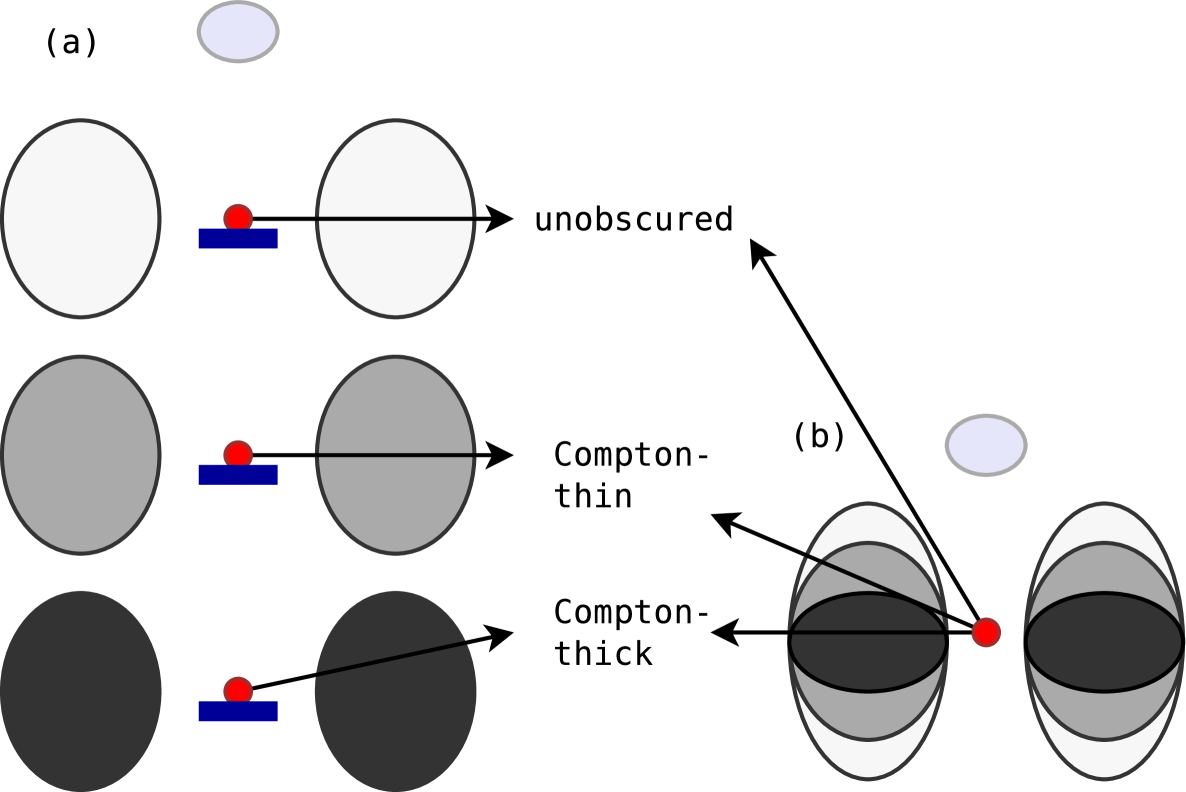
The geometry of the obscurer in the deepest field to date is thus, from the point of view of X-ray spectra, compatible with two simple scenarios illustrated in Figure 12: (a) Per-source density variations of a constant-density torus, with an accretion disk contributing extra reflection in some sources or (b), following the unification scheme, a torus with a column density gradient where the LOS obscuration depends on the viewing angle and the observed additional reflection originates in denser regions of the torus. In both scenarios, ionised clouds can scatter intrinsic radiation past the torus.
Acknowledgements.
JB thanks Farhan Feroz for proofreading the methodology section. Remaining errors are JB’s. JB acknowledges financial support through a Max-Planck-Gesellschaft stipend. We also thank the builders and operators of Chandra. This research has made use of software provided by the Chandra X-ray Center (CXC) in the application package CIAO.References
- Aird et al. (2010) Aird, J., Nandra, K., Laird, E. S., et al. 2010, MNRAS, 401, 2531
- Akaike (1974) Akaike, H. 1974, Automatic Control, IEEE Transactions on, 19, 716
- Akylas et al. (2012) Akylas, A., Georgakakis, A., Georgantopoulos, I., Brightman, M., & Nandra, K. 2012, A&A, 546, A98
- Alexander & Hickox (2012) Alexander, D. M. & Hickox, R. C. 2012, New A Rev., 56, 93
- Antonucci (1993) Antonucci, R. 1993, ARA&A, 31, 473
- Antonucci (1982) Antonucci, R. R. J. 1982, Nature, 299, 605
- Antonucci & Miller (1985) Antonucci, R. R. J. & Miller, J. S. 1985, ApJ, 297, 621
- Arnouts et al. (1999) Arnouts, S., Cristiani, S., Moscardini, L., et al. 1999, MNRAS, 310, 540
- Ashby et al. (2013) Ashby, M. L. N., Willner, S. P., Fazio, G. G., et al. 2013, ApJ, 769, 80
- Baganoff (1999) Baganoff, F. 1999, ACIS On-orbit Background Rates and Spectra from Chandra OAC Phase 1, ACIS Memo 162, Massachusetts Institute of Technology, Centerfor Space Research
- Bayarri & Castellanos (2008) Bayarri, M. J. & Castellanos, M. E. 2008, ArXiv e-prints
- Brightman & Nandra (2011) Brightman, M. & Nandra, K. 2011, MNRAS, 413, 1206
- Brightman et al. (2013) Brightman, M., Silverman, J. D., Mainieri, V., et al. 2013, MNRAS, 433, 2485
- Brightman & Ueda (2012) Brightman, M. & Ueda, Y. 2012, MNRAS, 423, 702
- Broos et al. (2010) Broos, P. S., Townsley, L. K., Feigelson, E. D., et al. 2010, ApJ, 714, 1582
- Budavári & Szalay (2008) Budavári, T. & Szalay, A. S. 2008, ApJ, 679, 301
- Burtscher et al. (2013) Burtscher, L., Meisenheimer, K., Tristram, K. R. W., et al. 2013, ArXiv e-prints
- Cardamone et al. (2010) Cardamone, C. N., van Dokkum, P. G., Urry, C. M., et al. 2010, ApJS, 189, 270
- Cash (1979) Cash, W. 1979, ApJ, 228, 939
- Comastri et al. (2002) Comastri, A., Vignali, C., Brusa, M., Hellas, & Hellas2XMM Consortia. 2002, in Astronomical Society of the Pacific Conference Series, Vol. 284, IAU Colloq. 184: AGN Surveys, ed. R. F. Green, E. Y. Khachikian, & D. B. Sanders, 235
- Damen et al. (2011) Damen, M., Labbé, I., van Dokkum, P. G., et al. 2011, ApJ, 727, 1
- de Rosa et al. (2012) de Rosa, A., Panessa, F., Bassani, L., et al. 2012, MNRAS, 420, 2087
- Efron et al. (2001) Efron, B., Gous, A., Kass, R., Datta, G., & Lahiri, P. 2001, Lecture Notes-Monograph Series, 208
- Fabian (1989) Fabian, A. C. 1989, in ESA Special Publication, Vol. 296, Two Topics in X-Ray Astronomy, Volume 1: X Ray Binaries. Volume 2: AGN and the X Ray Background, ed. J. Hunt & B. Battrick, 1097–1104
- Fabian (1999) Fabian, A. C. 1999, MNRAS, 308, L39
- Feroz et al. (2009) Feroz, F., Hobson, M. P., & Bridges, M. 2009, MNRAS, 398, 1601
- Ferrarese et al. (1996) Ferrarese, L., Ford, H. C., & Jaffe, W. 1996, ApJ, 470, 444
- Freeman et al. (2001) Freeman, P., Doe, S., & Siemiginowska, A. 2001, in Society of Photo-Optical Instrumentation Engineers (SPIE) Conference Series, Vol. 4477, Society of Photo-Optical Instrumentation Engineers (SPIE) Conference Series, ed. J.-L. Starck & F. D. Murtagh, 76–87
- Gaskell et al. (2008) Gaskell, C. M., Goosmann, R. W., & Klimek, E. S. 2008, Mem. Soc. Astron. Italiana, 79, 1090
- Georgakakis et al. (2013) Georgakakis, A., Carrera, F., Lanzuisi, G., et al. 2013, ArXiv e-prints
- Georgantopoulos & Georgakakis (2005) Georgantopoulos, I. & Georgakakis, A. 2005, MNRAS, 358, 131
- George & Fabian (1991) George, I. M. & Fabian, A. C. 1991, MNRAS, 249, 352
- Gierliński & Done (2004) Gierliński, M. & Done, C. 2004, MNRAS, 349, L7
- Gondhalekar et al. (1997) Gondhalekar, P. M., Rouillon-Foley, C., & Kellett, B. J. 1997, MNRAS, 288, 260
- Grogin et al. (2012) Grogin, N. A., Rajan, A., Donley, J. L., et al. 2012, in American Astronomical Society Meeting Abstracts, Vol. 220, American Astronomical Society Meeting Abstracts 220, 335.23
- Guainazzi & Bianchi (2007) Guainazzi, M. & Bianchi, S. 2007, MNRAS, 374, 1290
- Guo et al. (2013) Guo, Y., Ferguson, H. C., Giavalisco, M., et al. 2013, ApJS, 207, 24
- Hopkins et al. (2009) Hopkins, P. F., Hickox, R., Quataert, E., & Hernquist, L. 2009, MNRAS, 398, 333
- Hsieh et al. (2012) Hsieh, B.-C., Wang, W.-H., Hsieh, C.-C., et al. 2012, ApJS, 203, 23
- Hunter (2007) Hunter, J. D. 2007, Computing In Science & Engineering, 9, 90
- Ilbert et al. (2006) Ilbert, O., Arnouts, S., McCracken, H. J., et al. 2006, A&A, 457, 841
- Ilbert et al. (2009) Ilbert, O., Capak, P., Salvato, M., et al. 2009, ApJ, 690, 1236
- Jeffreys (1961) Jeffreys, H. 1961, International series of monographs on physics.
- Jones et al. (2001–) Jones, E., Oliphant, T., Peterson, P., et al. 2001–, SciPy: Open source scientific tools for Python
- King (2005) King, A. 2005, ApJ, 635, L121
- King (2010) King, A. R. 2010, MNRAS, 408, L95
- Koekemoer et al. (2011) Koekemoer, A. M., Faber, S. M., Ferguson, H. C., et al. 2011, ApJS, 197, 36
- Komatsu et al. (2011) Komatsu, E., Smith, K. M., Dunkley, J., et al. 2011, ApJS, 192, 18
- Kormendy & Ho (2013) Kormendy, J. & Ho, L. C. 2013, ARA&A, 51, 511
- Krolik & Kallman (1987) Krolik, J. H. & Kallman, T. R. 1987, ApJ, 320, L5
- Kullback & Leibler (1951) Kullback, S. & Leibler, R. A. 1951, The Annals of Mathematical Statistics, 22, 79
- Laird et al. (2009) Laird, E. S., Nandra, K., Georgakakis, A., et al. 2009, ApJS, 180, 102
- Levenberg (1944) Levenberg, K. 1944, Quart. Applied Math., 2, 164
- Magdziarz & Zdziarski (1995) Magdziarz, P. & Zdziarski, A. A. 1995, MNRAS, 273, 837
- Marquardt (1963) Marquardt, D. 1963, Journal of the Society for Industrial and Applied Mathematics, 11, 431
- Matt (2002) Matt, G. 2002, MNRAS, 337, 147
- Morrison & McCammon (1983) Morrison, R. & McCammon, D. 1983, ApJ, 270, 119
- Murphy & Yaqoob (2009) Murphy, K. D. & Yaqoob, T. 2009, MNRAS, 397, 1549
- Mushotzky (2004) Mushotzky, R. 2004, in Astrophysics and Space Science Library, Vol. 308, Supermassive Black Holes in the Distant Universe, ed. A. J. Barger, 53
- Nandra & George (1994) Nandra, K. & George, I. M. 1994, MNRAS, 267, 974
- Nandra et al. (2005) Nandra, K., Laird, E. S., Adelberger, K., et al. 2005, MNRAS, 356, 568
- Nandra et al. (2007) Nandra, K., O’Neill, P. M., George, I. M., & Reeves, J. N. 2007, MNRAS, 382, 194
- Nandra & Pounds (1994) Nandra, K. & Pounds, K. A. 1994, MNRAS, 268, 405
- Perola et al. (2002) Perola, G. C., Matt, G., Cappi, M., et al. 2002, A&A, 389, 802
- Protassov et al. (2002) Protassov, R., van Dyk, D. A., Connors, A., Kashyap, V. L., & Siemiginowska, A. 2002, ApJ, 571, 545
- Rangel et al. (2013a) Rangel, C., Nandra, K., Laird, E. S., & Orange, P. 2013a, MNRAS
- Rangel et al. (2013b) Rangel, C., Nandra, K., Laird, E. S., & Orange, P. 2013b, MNRAS, 428, 3089
- Richstone et al. (1998) Richstone, D., Ajhar, E. A., Bender, R., et al. 1998, Nature, 395, A14
- Risaliti et al. (1999) Risaliti, G., Maiolino, R., & Salvati, M. 1999, ApJ, 522, 157
- Ross & Fabian (1993) Ross, R. R. & Fabian, A. C. 1993, MNRAS, 261, 74
- Salvato et al. (2009) Salvato, M., Hasinger, G., Ilbert, O., et al. 2009, ApJ, 690, 1250
- Salvato et al. (2011) Salvato, M., Ilbert, O., Hasinger, G., et al. 2011, ApJ, 742, 61
- Schwarz (1978) Schwarz, G. 1978, Ann. Stat., 6, 461
- Severgnini et al. (2003) Severgnini, P., Caccianiga, A., Braito, V., et al. 2003, A&A, 406, 483
- Shankar et al. (2004) Shankar, F., Salucci, P., Granato, G. L., De Zotti, G., & Danese, L. 2004, MNRAS, 354, 1020
- Shankar et al. (2009) Shankar, F., Weinberg, D. H., & Miralda-Escudé, J. 2009, ApJ, 690, 20
- Silk & Rees (1998) Silk, J. & Rees, M. J. 1998, A&A, 331, L1
- Sinharay & Stern (2003) Sinharay, S. & Stern, H. S. 2003, Journal of Statistical Planning and Inference, 111, 209 , special issue I: Model Selection, Model Diagnostics, Empirical Bayes and Hierarchical Bayes
- Skilling (2004) Skilling, J. 2004, in AIP Conference Proceedings, Vol. 735, 395
- Stark et al. (1992) Stark, A. A., Gammie, C. F., Wilson, R. W., et al. 1992, ApJS, 79, 77
- Sunyaev & Titarchuk (1980) Sunyaev, R. A. & Titarchuk, L. G. 1980, A&A, 86, 121
- Thompson et al. (2001) Thompson, A., Vaughan, D., et al. 2001, X-ray data booklet (Lawrence Berkeley National Laboratory, University of California Berkeley, CA)
- Tozzi et al. (2006) Tozzi, P., Gilli, R., Mainieri, V., et al. 2006, A&A, 451, 457
- Treister et al. (2004) Treister, E., Urry, C. M., Chatzichristou, E., et al. 2004, ApJ, 616, 123
- Turner et al. (1997) Turner, T. J., George, I. M., Nandra, K., & Mushotzky, R. F. 1997, ApJS, 113, 23
- Turner & Pounds (1989) Turner, T. J. & Pounds, K. A. 1989, MNRAS, 240, 833
- Ueda et al. (2007) Ueda, Y., Eguchi, S., Terashima, Y., et al. 2007, ApJ, 664, L79
- van der Marel & van den Bosch (1998) van der Marel, R. P. & van den Bosch, F. C. 1998, AJ, 116, 2220
- van Dyk et al. (2001) van Dyk, D. A., Connors, A., Kashyap, V. L., & Siemiginowska, A. 2001, ApJ, 548, 224
- Wilk & Gnanadesikan (1968) Wilk, M. B. & Gnanadesikan, R. 1968, Biometrika, 55, pp. 1
- Wilks (1938) Wilks, S. 1938, The Annals of Mathematical Statistics, 60
- Xue et al. (2011) Xue, Y. Q., Luo, B., Brandt, W. N., et al. 2011, ApJS, 195, 10
- Zdziarski et al. (2000) Zdziarski, A. A., Poutanen, J., & Johnson, W. N. 2000, ApJ, 542, 703
Appendix A Goodness-of-Fit of the Background model

In the large, bottom panel we present the corresponding Q–Q (quantile-quantile) plot. For each energy , the model counts predicted and the counts observed below are recorded on the plot. The grey dashed line is where data and model would perfectly agree. Model 1 (blue solid top line) follows this line very closely, and thus can be considered a good model. Model 2 (red solid bottom line) deviates from the grey dashed line at , indicating that a feature in the data may be missing in the model. The shape and size of the deviation also indicates the shape of the needed feature. The significance of the feature can be tested using model selection. Here, the AIC shows that the feature at is necessary , but adding the more complicated feature at is not (see text in Appendix A for details).
We intend to demonstrate that the used background description is a good model. To this end, we present a goodness of fit (GoF) methodology for X-ray spectra. We use QQ plots for model discovery and the AIC model comparison method to test for the significance of model improvements, although any of the model comparison methods introduced in Section 5.2 could be chosen. We demonstrate the method using a background source spectrum and our best fit, comparing it to a simplified model. In our analysis, every spectrum is fitted individually to accommodate the diversity of background spectra.
A.1 Background model definition
We present “Model 1”, which is our final Gaussian mixture model with a constant base continuum:
To model the rise in the soft energies two Gaussians (called “softend” and “softsoftend”) are used of widths and at centred at . Another five Gaussian lines describe the spectral bumps due to e.g. transition lines of the detector material. These are centred around 1.486 (), 1.739 (), 2.142 (), 7.478 (), 9.713 (; all in keV). A feature at possibly composed of / lines is modelled by three further Gaussians at , , . We allow all centres to vary within . The parameters start from reasonable guesses and are optimised as long as the fit statistic (C-Stat) improves.
Figure 13 shows the comparison between data and model for a source with the sequential number 318 in the catalogue. This source has 3380 counts and was chosen because it constitutes an intermediate case between the most high-count spectra with many peculiarities and low-count spectra with almost no visible features. The final parameter values after fitting are shown in Table 5 (middle column).
| Source | 318 | 179 |
|---|---|---|
| line1.ampl | 413 | 511 |
| line1.fwhm | 0.0329 | 0.0162 |
| line1.pos | 1.475 | 1.49 |
| line2.ampl | 0 | 74.7 |
| line2.fwhm | 0.1 | 0.002 |
| line2.pos | 1.84 | 1.82 |
| line3.ampl | 420 | 581 |
| line3.fwhm | 0.1 | 0.0827 |
| line3.pos | 2.16 | 2.16 |
| line4.ampl | 3769 | 1159 |
| line4.fwhm | 0.0257 | 0.0768 |
| line4.pos | 7.48 | 7.49 |
| line5.ampl | 1446 | 42.9 |
| line5.fwhm | 0.002 | 0.102 |
| line5.pos | 8.10 | 8.07 |
| line6.ampl | 97.1 | 280 |
| line6.fwhm | 0.4 | 0.0793 |
| line6.pos | 8.37 | 8.25 |
| line7.ampl | 111.5 | 6656 |
| line7.fwhm | 0.002 | 0.002 |
| line7.pos | 8.47 | 8.47 |
| line8.ampl | 1993 | 2225 |
| line8.fwhm | 0.1 | 0.0886 |
| line8.pos | 9.72 | 9.71 |
| softend.ampl | 21092 | 21824 |
| softend.fwhm | 2.0 | 2.6 |
| softend.pos | 1.0 | 1.0 |
| softsoftend.ampl | 72642 | 78711 |
| softsoftend.fwhm | 0.325 | 0.638 |
| softsoftend.pos | 0.167 | 0.243 |
A.2 Goodness of Fit and Model discovery
For comparison, we present Model 2 which has several Gaussians disabled, namely the one centred at (line 3) and the three between (line 5-7). The intent is to compare methods evaluating whether Model 2 is a good model, where it deviates from the data, and whether the deviation is significant.
The classic method is to plot the data, model and the residuals. This is shown in the upper left panel of Figure 13 for the un-binned data and model, with the residuals below. The upper right panel shows the same, but with adaptive binning requiring 20 counts in each bin. The feature at is visible immediately, while the feature at is less striking.
We present an alternative method of analysing the quality of a model: the Q–Q plot, shown in the large lower panel. For each energy , the model counts predicted and the counts observed below are recorded on the plot. Here the counts are shown, while statisticians typically use quantiles, i.e. the fraction of observations that lie below a quantity. This does not influence the main point, namely the shape of the curve. The grey dashed line is where data and model would perfectly agree. A steeper curve means the model predicts more counts than observed, while a shallower curve indicates an excess of observed counts.
Model 1 (blue solid top line) follows this line very closely, and thus can be considered a good model. Model 2 (red solid bottom line) deviates from the grey dashed line at , indicating that a feature in the data is not modelled. Above , the line is parallel to Model 1, indicating no further difference. This means the feature is confined to this energy range. With a bit of practise one can also see that the difference required to bring the lines into agreement looks like the cumulative distribution of a Gaussian (a S-shape rather than e.g. a straight line for a flat distribution). Another, but more subtle, deviation is visible between . This is highlighted using the green solid middle line which does model the feature.
Having found a good model, and slightly worse, simpler models, we can now test whether the improvement is significant. For instance, it seems doubtful that the minute feature at justifies modelling with 3 Gaussian components (9 parameters). For this, we employ the AIC, which punishes the difference in the likelihood (C-stat) by adding twice the number of parameters. As (Model 2 vs Model 1, red text), the worsening is significant. But if we only remove the feature at , the AIC decreases due to the simplification of the model (green text). Thus, in this source, the feature can be ignored. However, in sources with more counts, it is required (see Figure 14 for one example).
The deviation between model and data can be summarised using GoF measures. The Kolmogorov-Smirnov measure, , records the largest deviation between the empirical cumulative distribution of observed counts (0 at the lowest energy, 1 at the highest), and the model cumulative distribution. Other measures, such as the ones used for the Cramér–von Mises test or the Anderson–Darling test take all deviations into account, not merely the largest. When many spectra are analysed in an automated fashion, the highest values can hint to problematic cases which require further, visual analysis.
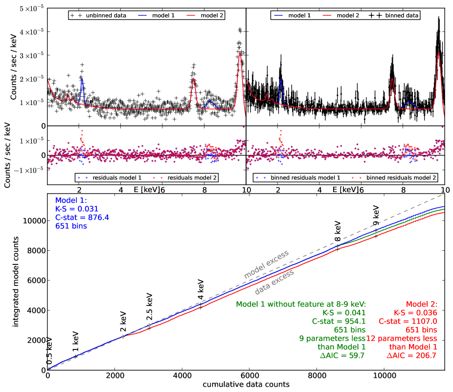
Appendix B Propagation of redshift uncertainty
It is common practise to use a redshift point estimator (best fit redshift) from photometric redshifts and analyse spectra with this value. In this work, in contrast, the redshift uncertainty from photometric redshift is propagated into the analysis of X-ray spectra in the form of a probability distribution on the redshift parameter. In this section, we discuss the differences between the approaches.
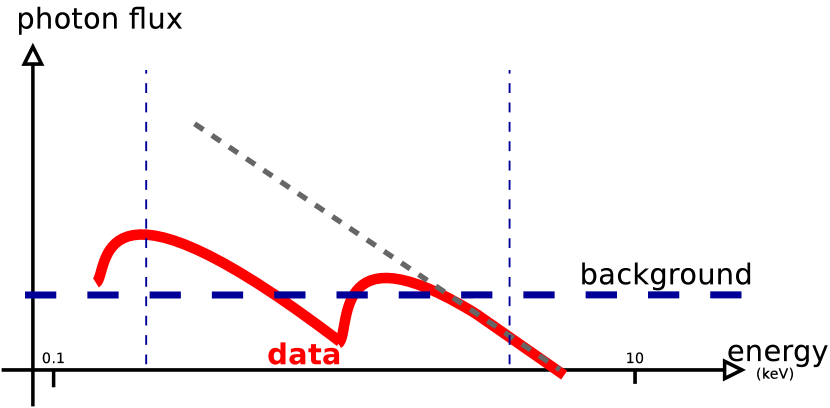
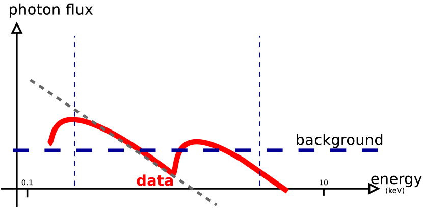
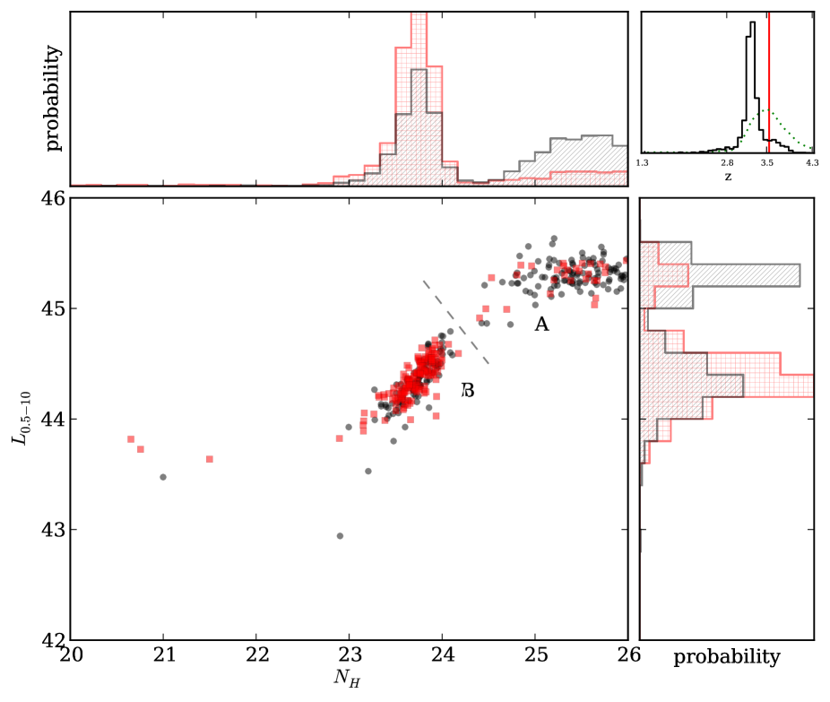
Two separated solutions are clearly visible and highlighted using the labels “A” for the highly obscured solution and “B” for the less obscured solution. The associated spectra are illustrated in Figure 15. The fixed redshift analysis has the highest likelihood at the less obscured solution. When given the freedom to vary the redshift parameter, the X-ray data have the highest likelihood at the highly obscured solution. Maximum Likelihood analysis methods thus may fail to account for the uncertainty (see text). The difference in results come from the freedom to move to a lower redshift, as can be seen in the upper right panel, where the black line shows the redshift posterior probability distribution. These results thus also show that redshift information can be improved using X-ray data (see Buchner et al. in prep).
We consider the source 551 in our catalogue and analyse its X-ray spectrum using the methodology laid out in this paper with the torus model. We perform the analysis twice, a) with the probability distribution from photometric redshifts and b) with the best fit photo-metric redshift. Figure 16 demonstrates how the different input redshifts (upper right panel) influence the results in the derived column density and intrinsic luminosity parameters (large panel). The Bayesian analysis shows that the parameter space is broad, and split to two distinct solutions (see lower left panel in Figure 16): a highly obscured solution and a less obscured solution. The maximum likelihood is in the less obscured solution for the fixed redshift value, but in the highly-obscured solution if the redshift distribution is used, because the likelihood improves when using a slightly lower value than the best fit redshift. The two solutions are strictly separated, i.e. an intermediate solution is ruled out. Common Maximum Likelihood methods, like fitting and error estimation by Fisher matrix or contour search, will fail to estimate the uncertainty correctly and hide the respectively other solution. Methods building on these results can therefore make false conclusions about e.g. the number of Compton-thick sources. The Bayesian inference method presented in this work can handle the separated solutions well and re-weighs them based on the redshift information given. The various methods are discussed and compared in Section 5.
Appendix C False discovery rate of model comparison methods
In this section, we compare the efficiency and error rate of model comparison methods.
On the one hand we consider methods based on the ratio of the highest likelihood, where, if the likelihood improves beyond a certain log-likelihood ratio threshold, the more complex model is accepted. The threshold may be dependent on the difference in the number of model parameters. In this general form, Wilks’ theorem, -test, -test, AIC and BIC methods are covered.
On the other hand, the Bayesian inference based on computing the evidence is considered, where, assuming a-priori equality, the Bayes factor is used to decide which model to use. In particular, when is greater than the threshold, Model 1 is accepted, while if is greater than the threshold, Model 2 is accepted. An important difference is that when the Bayesian inference can conclude that not enough information to make a decision.
C.1 Nested Problems
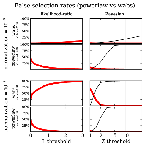
Considering the sum of thick red lines in panel pairs, the Bayesian model selection has a false selection rate below at the marked threshold, which can not be achieved using likelihood-ratios regardless of the threshold chosen. The Bayesian model selection may decline to decide due to insufficient discriminatory power of the data (thin black line). This is the case for the faint normalisations (bottom four panels), where the likelihood-ratio methods remain with the simpler model (yielding an error of ). In the brighter normalisations (upper right panels), the Bayesian method beyond a threshold of declines to distinguish when the powerlaw model was used to generate the data. This is a consequence of the degeneracy between the nested powerlaw and wabs models. Thus for nested models, a lower threshold, such as can be appropriate. When considering the efficiency only, the likelihood ratio based method yields more correct decisions, as the Bayesian method declines to choose very often. However, one may also remain with the simpler model, in which case the results would be comparable.
We generate 2000 spectra each based on the powerlaw and wabs input model. We assume a photon index of , redshift and column density (for wabs). The normalisation of the source power-law at 1 keV in is set to either or (1000 simulated spectra each). A fixed, flat background with is used. We re-use the exposure time, ARF and RMF of Source 179 to produce realistic, low-count spectra.
We analyse all simulated X-ray spectra in the band using the methodology laid out in this paper, once with the powerlaw and once with the wabs model. We also store the maximum likelihood (best fit). We apply model selection (Bayesian and likelihood-ratio-based) between powerlaw and the more complicated model wabs, and record the number of false choices (e.g. wabs was preferred, although powerlaw was used for generating the spectrum). These results shown in Figure 17 using thick red lines. For the Bayesian model selection, we also record the number of cases where no significant preference was found (black lines).
The Bayesian model selection has a false selection rate below at the marked threshold, which can not be achieved by likelihood-ratio based methods regardless of the threshold chosen. The Bayesian model selection may decline to decide due to insufficient discriminatory power of the data (thin black line). When considering the efficiency only, the likelihood ratio based method yields more correct decisions, as the Bayesian method declines to choose very often. However, one may also remain with the simpler model, in which case the results would be comparable.
C.2 Non-nested problems
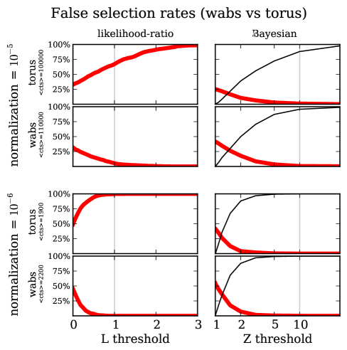
We now consider a non-nested model selection problem, applying the same methodology. We select between the models wabs and torus – neither is a special case of the other. We apply likelihood-ratio based methods using wabs as the null hypothesis, and only select torus when the likelihood-ratio threshold is exceeded. These results are presented in a similar fashion as above in Figure 18. The panels show higher normalisations, as the models are more subtle in their differences.
C.3 Conclusion
To summarise the Figures 17 and 18, error rates below can be achieved using the in the Bayesian model selection, with a threshold of e.g. . It should be clear that a Bayes factor of is actually a quite conservative choice, and does not necessarily refer to a false positive rate of 1 in 10, but a much lower value. This point has been appreciated in the literature before: Efron et al. (2001) show that the Bayes factor scale by Jeffreys (1961) is probably overly conservative.
In contrast, methods based on the likelihood-ratio always have higher error rates than regardless of the chosen threshold. This is due to the procedure remaining with the simpler model if the data has insufficient discriminatory power. The Bayesian method has the benefit of recognising these cases and can decline to decide. It should be stressed again that several likelihood ratio based methods are not valid for non-nested problems (Wilks’ theorem, F-test, -test, likelihood-ratio test), although e.g. the AIC is. Furthermore, all likelihood ratio based methods are not valid at testing against the border of the parameter space (e.g. powerlaw is a special case of wabs with minimal ). This is discussed further in Section 5.2. These results demonstrate that even if a valid method based on the likelihood ratio was introduced, it would perform poorly in the shown cases.