Conformations, Transverse Fluctuations and Crossover Dynamics of a Semi-Flexible Chain in Two Dimensions

Abstract

We present a unified scaling description for the dynamics of monomers of a semiflexible chain under good solvent condition in the free draining limit. We consider both the cases where the contour length $L$ is comparable to the persistence length $\ell_{p}$ and the case $L\gg\ell_{p}$. Our theory captures the early time monomer dynamics of a stiff chain characterized by $t^{3/4}$ dependence for the mean square displacement(MSD) of the monomers, but predicts a first crossover to the Rouse regime of $t^{2\nu/{1+2\nu}}$ for $\tau_{1}\sim\ell_{p}^{3}$, and a second crossover to the purely diffusive dynamics for the entire chain at $\tau_{2}\sim L^{5/2}$. We confirm the predictions of this scaling description by studying monomer dynamics of dilute solution of semi-flexible chains under good solvent conditions obtained from our Brownian dynamics (BD) simulation studies for a large choice of chain lengths with number of monomers per chain N = 16 - 2048 and persistence length $\ell_{p}=1-500$ Lennard-Jones (LJ) units. These BD simulation results further confirm the absence of Gaussian regime for a 2d swollen chain from the slope of the plot of $\langle R_{N}^{2}\rangle/2L\ell_{p}\sim L/\ell_{p}$ which around $L/\ell_{p}\sim 1$ changes suddenly from $\left(L/\ell_{p}\right)\rightarrow\left(L/\ell_{p}\right)^{0.5}$, also manifested in the power law decay for the bond autocorrelation function disproving the validity of the WLC in 2d. We further observe that the normalized transverse fluctuations of the semiflexible chains for different stiffness $\sqrt{\langle l_{\bot}^{2}\rangle}/L$ as a function of renormalized contour length $L/\ell_{p}$ collapse on the same master plot and exhibits power law scaling $\sqrt{\langle l_{\bot}^{2}\rangle}/L\sim(L/\ell_{p})^{\eta}$ at extreme limits, where $\eta=0.5$ for extremely stiff chains ($L/\ell_{p}\gg 1$), and $\eta=-0.25$ for fully flexible chains. Finally, we compare the radial distribution functions obtained from our simulation studies with those obtained analytically.

I Introduction

Macromolecules adsorbed on substrate surfaces occur in many different contexts, from materials science to biophysics, e.g., biomolecules interacting with cell membranes. Hence the understanding of conformations and dynamics of macromolecules in such a (quasi-) two-dimensional geometry has been of long-standing interest deGennes_1987 ; Fleer ; Eisenriegler ; Netz_2003 . Note also that many methods to characterize polymer conformations experimentally, e.g., electron microscopy Takabayashi ; Stokke ; Trachtenberg ; Bednar ; Agaskova ; Papadopoulos ; Lehman , atomic force microscopy (AFM) Hansma ; Yoshinaga ; Valle ; Moukhtar_PRL_2005 ; Rechendorff ; Langowski ; Moukhtar_2010 , fluorescence microscopy of suitably labelled biopolymers Maier_PRL_1999 ; Maier_2000 , require that these macromolecules are attached to a substrate. In this context, considerations of macromolecules confined to a strictly two-dimensional geometry are of interest, at least as a limiting case. The same statement holds when one considers macromolecules confined to nanoslits with non-adsorbing walls, a topic that also has found much recent interest.

While the statistical mechanics of completely flexible polymers in $d=2$ dimensions has been studied extensively since a long time and is well understood deGennes_book ; Sokal , under many circumstances it should be taken into account that macromolecules are stiff and not flexible on small scales Flory ; Grosberg ; Rubinstein . This is true both for simple synthetic polymers e.g., polystyrene, alkane chains, etc., and for various biopolymers, e.g., double-stranded (ds) and single stranded (ss) DNA, polysaccharides, proteins, etc. Parry . Apart from very stiff polymers (e.g., Actin, Titin, microtubules, etc.) the “persistence length $\ell_{p}$ Flory ; Grosberg ; Rubinstein ; Parry ; Hsu_Macro_2010 characterizing the stiffness typically is much less than the contour length $L$ of a macromolecule, and the crossover from rod-like behavior to the behavior of flexible polymers needs to be considered. As is well-known, the scales of interest range from the sub-nanometer scale to the micrometer scale Binder_book ; Thirumalai_Nature_2011 , and hence in the theoretical modeling coarse-grained models must be used Binder_book ; Thirumalai_Nature_2011 ; Hsu_Macro_Simul_2011 .

In the present work, we wish to address the problem of polymer conformation and dynamics for semi-flexible polymers in two dimensions, using Molecular Dynamics simulations of a bead-spring type model with a bond angle potential by which we can control the stiffness of the chains over a wide range. We note that the standard analytical coarse-grained description in terms of the Kratky-Porod Kratky ; Harris model for wormlike chains in $d=2$ dimensions is not very useful, since it neglects excluded volume effects completely, although they are known to be very important in $d=2$ Hsu_EPL_2011 . A study of semiflexible polymers in terms of a lattice model Hsu_EPL_2011 ; Hsu_JCP_2012_1 ; Hsu_JCP_2012_2 ; Hsu_Soft_2013 is expected to yield valid results for universal properties of semiflexible polymer, i.e., on length scales much larger than the persistence length; but on smaller scales it can describe only stiffness of the type similar to that of alkane chains, where $\ell_{p}$ is of the order of the typical length of “all trans” sequences, in between monomers taking a gauche ($g\pm$) minimum in the torsional potential. For such cases e.g., dsDNA we expect that the (small) flexibility of the macromolecules is due to fluctuations in bond lengths and bond angles, rather than disorder in the population of states in the torsional potential, and then the present off-lattice model is more realistic. In addition, the lattice work Hsu_EPL_2011 ; Hsu_JCP_2012_1 ; Hsu_JCP_2012_2 ; Hsu_Soft_2013 applying the pruned enriched Rosenbluth method (PERM) Grassberger_1997 ; Hsu_Stat_2011 could not address the dynamics of the chains at all. Previous work on the dynamics of single semiflexible chains in dilute solution Pincus_MM_1980 ; Harnau2 ; Kroy_PRE_1997 ; Shusterman_PRL_2004 ; Petrov ; Netz_EPL_2009 ; Hinczewski ; Hinczewski_PhysicaA ; Steinhauser has focused on the case $d=3$ almost exclusively, and most of the work Pincus_MM_1980 ; Harnau2 ; Kroy_PRE_1997 ; Shusterman_PRL_2004 ; Petrov ; Netz_EPL_2009 ; Hinczewski ; Hinczewski_PhysicaA has studied the effect of hydrodynamic (HD) interactions mediated by the solvent. Assuming that the substrate surface provides a stick boundary condition with respect to solvent fluid flow, one can show Winkler that HD interactions are essentially screened, and hence are ignored here (as well as in our preliminary communication where a small part of our results were presented Huang_epl ) from the outset.

While the Kratky-Porod Worm-like-chain (WLC) Model has been found to be grossly inadequate to describe a semiflexible chain in 2d, vast amounts of analytical and numerical work have been accumulated using the WLC model as the starting point Harnau1 ; Harnau2 ; Winkler_JCP_2003 . Recent experimental results of confined biopolymers on a 2d substrate are also analyzed using the well known results of WLC model Moukhtar_PRL_2005 . Therefore, in the following section we summarize the main results of the WLC model which we will revisit in the subsequent sections to compare our simulation results. The organization of the paper is as follows. In the next section we introduce the WLC model. Next in Sec. III a scaling theory is derived where we show that monomer dynamics of a semiflexible polymer exhibits a double crossover as a function of time. We then introduce the bead spring model for a semiflexible chain in Sec. IV. The results of BD simulation are presented in Sec. V, which is divided into two sub-sections: The equilibrium properties are presented in Sec. V.1; in Sec. V.2 among other results we validate the predictions of the scaling theory using (BD) simulation for chains of different length and stiffness.

II Kratky-Porod Worm-like-chain (WLC) Model

The Hamiltonian corresponding to the bending energy for the WLC model is given by

$$\mathcal{H}=\frac{\kappa}{2}\int_{0}^{L}\left(\frac{\partial^{2}\mathbf{r}}{\partial s^{2}}\right)^{2}ds,$$ (1)

where $\mathbf{r}(s)$ is the position vector of a mass point, $L$ is the inextensible contour length, $\kappa$ is the bending rigidity, and the integration is carried out along the contour $s$ Rubinstein ; Doi . Using symmetry arguments for the free energy it can be shown Landau that the chain persistence length $\ell_{p}$ for a WLC in 2d and 3d are given by

The model has been studied quite extensively applying path integral and other techniques Harnau1 ; Winkler_JCP_2003 ; Yamakawa ; Wilhelm_PRL_1996 and exact expressions of various moments of the distribution of monomer distances along the chain have been worked out. The end-to-end distance in the WLC model is given by Rubinstein

$$\frac{\langle R_{N}^{2}\rangle}{L^{2}}=\frac{2\ell_{p}}{L}\left(1-\frac{\ell_{p}}{L}[1-\exp(-L/\ell_{p})]\right).$$ (3)

In the limit $\ell_{p}\ll L$ one gets $\langle R_{N}^{2}\rangle=2\ell_{p}L$ and the chain behaves like a Gaussian coil; for $\ell_{P}\gg L$, $\langle R_{N}^{2}\rangle=L^{2}$ and the chain behaves like a rod. Evidently the model neglects the excluded volume (EV) (Eqn. 14 of the bead-spring model in Sec.-IV) interaction and hence interpolates between rod and Gaussian limits only.

The WLC model can be viewed as a limiting case of a freely rotating chain Rubinstein , where the correlation between bond vectors $\vec{b_{i}}$ and $\vec{b}_{i+s}$ is assumed to follow

$$\left<\vec{b}_{i}\cdot\vec{b}_{i+s}\right>=b^{2}\exp(-s/\ell_{p}),$$ (4)

where $|\vec{b_{i}}|=|\vec{b}_{i+s}|=b$ and the characteristic length is defined as the persistence length $\ell_{p}$. From Eqn. 4 it then immediately follows that $\ell_{p}$ can be calculated from the bond angle $\cos\theta=\hat{b}_{i}\cdot\hat{b}_{i+1}$, where $\hat{b}_{i}$ is the unit vector of the corresponding bond vector $\vec{b}_{i}$ as follows:

$$\ell_{p}=-\frac{1}{\ln\left(\cos\theta\right)}.$$ (5)

Likewise, dynamics of the WLC model have been explored using Langevin type of equation Granek_1997 ; Maggs_MM_1993 ; Kroy_PRE_1997 ; Wilhelm_PRL_1996 ; Bullerjahn_EPL_2011 . One can expect that the dynamics of a stiff chain will be dominated by transverse fluctuations (bending modes) Winkler_JCP_2003 and that the short time dynamics will be governed by the chain persistence length. Indeed a relaxation dynamics using the WLC Hamiltonian (Eqn. 1) approach yields an expression for fluctuation

$$\langle\left(\Delta h\right)^{2}\rangle\sim\ell_{p}^{-0.25}t^{0.75}.$$ (6)

which crosses over to simple diffusion at late time Granek_1997 ; Maggs_MM_1993 . As we will see later from our results that even for a Gaussian chain a more “complete theory” should have captured an intermediate regime characterized by a growth law $t^{0.5}$ for a fully flexible chain for an intermediate time when the fluctuation becomes of the order of radius of gyration of the chain. However, the Langevin theories for the WLC chain did not describe this regime.

III Scaling description

We first develop the scaling description for the dynamics of a two dimensional semiflexible chain in the free draining limit. The free draining limit is of particular interest in 2d because it often satisfies the experimental conditions, such as DNA confined in a 2d substrate where the effect of hydrodynamics is negligible. For a WLC several theories based on Langevin dynamics have been developed most of which indicate a $t^{0.75}$ dependence of the transverse fluctuation of the MSD $g_{1}(t)$ (see Eqn. 26a) with time $t$ for the stiff chain. Therefore, we start with the Eqn. 7 below derived by Granek Granek_1997 and Farge and Maggs Maggs_MM_1993 using a Langevin dynamics framework for the WLC Hamiltonian

$$g_{1}(t)=b^{2}\left(b/\ell_{p}\right)^{1/4}\left(Wt\right)^{3/4},$$ (7)

where $W$ is the monomer reorientation rate. Prefactors of order unity are omitted throughout Comment_g1 . For early time the monomer dynamics will be independent of the chain length $N$ until the fluctuations in monomer position become of the order of $\ell_{p}$. Therefore, denoting the time when the first crossover occurs as $\tau_{1}$ and substituting $g_{1}=\ell_{p}^{2}$ and $t=\tau_{1}$ in Eqn. 7 we immediately get

$$W\tau_{1}=\left(\ell_{p}/b\right)^{3}.$$ (8)

For $0<t\leq W^{-1}(\ell_{p}/b)^{3}$ the monomer dynamics is described by $g_{1}(t)\sim t^{0.75}$ according to Eqn. 7 until $g_{1}(t)=\ell_{p}^{2}$ at time $W^{-1}(\ell_{p}/b)^{3}$. The width of this region is independent of $N$ and solely a function of $\ell_{p}$ (see Fig. 1).

For $\tau_{1}<t<\tau_{2}$ the dynamics is governed by the Rouse relaxation of monomers of a fully flexible EV chain in 2d characterized by $g_{1}(t)\propto t^{2\nu/(1+2\nu)}=t^{0.6}$. $\tau_{2}$ characterizes the onset of the purely diffusive regime when $g_{1}(\tau_{2})=\langle R_{N}^{2}\rangle$ Grest_Kremer_PRA_1986 . Recall that the exponent $\nu$ that describes the scaling of the end-to-end distance $\vec{R}_{N}$ according to $\langle R_{N}^{2}\rangle\propto N^{2\nu}$ is $\nu=\frac{3}{4}$ in 2d.

Figure 1: Theoretical scaling for $(N,\kappa)\equiv(512,2)$, $(512,32)$(a) and $(N,\kappa)\equiv(128,32)$, $(1024,32)$(b). Blue (red) symbols, solid and dashed lines correspond to $g_{1}(t)\sim t^{0.75}$($g_{1}\sim t^{0.60}$), black dashed, solid lines correspond to $g_{3}(t)\sim t$. Here the power laws Eqn. 7,  10 and 13 are plotted, using units of $b=1$, $l_{p}=2\kappa/k_{B}T$, $W=1$. The width of each region shows how these regimes depend on $\ell_{p}$ and $N$. Note that in reality we expect a very gradual change of slope on the log-log plot at both crossover times, rather than sharp kinks.

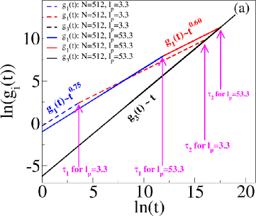
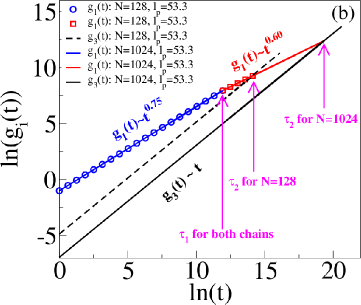
Note that when we increase the stiffness of the chain at fixed chain length, the times $\tau_{1}$ and $\tau_{2}$ can be made to coincide; this happens for $L=Nb=\ell_{p}$, as expected: when the contour length and the persistence length are of the same order, the regime described by Eqn. 10 is no longer present. We will verify the time dependence of $g_{1}$ at various regimes from BD simulations.

We then obtain $\tau_{2}$ as follows:

$$g_{1}(t)=\ell_{p}^{2}\left(t/\tau_{1}\right)^{3/5}\mathrm{~{}~{}~{}~{}~{}~{}for~{}~{}}t>\tau_{1}.$$ (9)

Substituting $\tau_{1}$ from Eqn. 8 in above

$$g_{1}(t)=b^{2}\left(\ell_{p}/b\right)^{1/5}\left(Wt\right)^{3/5},\mathrm{~{}~{}for~{}~{}}\tau_{1}<t<\tau_{2}.$$ (10)

At $t=\tau_{2}$

$$g_{1}(t=\tau_{2})=\langle R_{N}^{2}\rangle=\ell_{p}^{1/2}L^{3/2}.$$ (11)

Substituting Eqn. 10 for $t=\tau_{2}$ we get

$$W\tau_{2}=\left(\ell_{p}/b\right)^{\frac{1}{2}}N^{5/2}.$$ (12)

We also note that the dynamics of the center of mass is given by

$$g_{3}(t)=b^{2}W\frac{t}{N}.$$ (13)

The “phase diagram” for the crossover dynamics in terms of $N$, and $\ell_{p}$ are shown in Fig. 1. Notice that for a stiffer chain the region for $\tau_{1}<t<\tau_{2}$ for which we predict $g_{1}(t)\sim t^{0.6}$ requires to study very long chains and therefore, is hard to see in simulation for a stiffer chain.

IV THE MODEL

We have used a bead spring model of a polymer chain with excluded volume, spring and bending potentials as follows Grest_Kremer_PRA_1986 . The excluded volume interaction between any two monomers is given by a short range Lennard-Jones (LJ) potential with cut off and shifted in its minimum.

$$U_{\mathrm{LJ}}(r) = 4\epsilon[{(\frac{\sigma}{r})}^{12}-{(\frac{\sigma}{r})}^{6}]+\epsilon\;\;\;\;\;\;\;\;\mathrm{for~{}~{}}r\leq 2^{1/6}\sigma$$ (14)

$$= 0\;\;\;\;\;\;\;\;\;\;\;\;\;\;\;\;\;\;\;\;\;\;\;\;\;\;\;\ \mathrm{for~{}~{}}r>2^{1/6}\sigma\;.$$

Here, $\sigma$ is the effective diameter of a monomer, and $\epsilon$ is the strength of the potential. The connectivity between neighboring monomers is modeled as a Finitely Extensible Nonlinear Elastic (FENE) spring with

$$U_{\mathrm{FENE}}(r)=-\frac{1}{2}kR_{0}^{2}\ln(1-r^{2}/R_{0}^{2})\;,$$ (15)

where $r$ is the distance between consecutive monomers, $k$ is the spring constant and $R_{0}$ is the maximum allowed separation between connected monomers Grest_Kremer_PRA_1986 . The chain stiffness is introduced by adding an angle dependent interaction between successive bonds as (Fig. 2)

$$U_{\mathrm{bend}}(\theta_{i})=\kappa(1-\cos\theta_{i}).$$ (16)

Here $\theta_{i}$ is the complementary angle between the bond vectors $\vec{b}_{i-1}=\vec{r}_{i}-\vec{r}_{i-1}$ and $\vec{b}_{i}=\vec{r}_{i+1}-\vec{r}_{i}$, respectively, as shown in Fig. 2. The strength of the interaction is characterized by the bending rigidity $\kappa$. Introducing unit tangent vector $\mathbf{t}_{i}=\frac{\partial\mathbf{r}_{i}}{\partial s}$ ($|\mathbf{t}_{i}|=1$) we note that the discretized version of Eqn. 1 can be written as

$$\mathcal{H}\approx\frac{\kappa}{2}b_{l}\sum_{i}\left(\frac{\mathbf{t}_{i+1}-\mathbf{t}_{i}}{b_{l}}\right)^{2} =\frac{\kappa}{2b_{l}}\sum_{i}\left(\mathbf{t}_{i+1}^{2}+\mathbf{t}_{i}^{2}-2\cos\theta_{i}\right)$$

$$=\frac{\kappa}{b_{l}}\sum_{i}\left(1-\cos\theta_{i}\right),$$ (17)

where $b_{l}=|\vec{b_{i}}|$ is the bond length in our simulation. Therefore, for fixed bond length Eqn. 16 represents the discrete version of the WLC model of Eqn. 1. Thus the EV effect introduced through Eqn. 14 are completely absent in the WLC model.

Figure 2: Bead-spring model of a polymer chain with bending angle $\theta_{i}$ subtended by the vectors $\vec{b}_{i-1}=\vec{r}_{i}-\vec{r}_{i-1}$ and $\vec{b}_{i}=\vec{r}_{i+1}-\vec{r}_{i}$.

We use the Langevin dynamics with the following equation of motion for the i^th monomer

$$m\ddot{\vec{r}}_{i}=-\nabla(U_{\mathrm{LJ}}+U_{\mathrm{FENE}}+U_{\mathrm{bend}})-\Gamma\vec{v}_{i}+\vec{R}_{i}.$$

Here $\Gamma$ is the monomer friction coefficient and $\vec{R}_{i}(t)$, is a Gaussian white noise with zero mean at a temperature T, and satisfies the fluctuation-dissipation relation:

$$<\,\vec{R}_{i}(t)\cdot\vec{R}_{j}(t^{\prime})\,>=4k_{B}T\Gamma\,\delta_{ij}\,\delta(t-t^{\prime})\;.$$

The reduced units of length, time and temperature are chosen to be $\sigma$, $\sigma\sqrt{\frac{m}{\epsilon}}$, and $\epsilon/k_{B}$ respectively. For the spring potential we have chosen $k=30$ and $R_{0}=1.5\sigma$, the friction coefficient $\Gamma=0.7$, the temperature is kept at $1.2/k_{B}$. The choice of the FENE potential along with the LJ interaction parameters ensures that the average bond-length in the bulk $\langle b_{l}\rangle=0.971$. With the choice of these parameters the probability of chain crossing is very low. We also find that the average bond-length $\langle b_{l}\rangle$ is almost independent of the range of chain stiffness parameter ($\kappa=0-320$) used in our simulation. Strictly speaking, the contour length $L$ is $L=\left(N-1\right)\langle b_{l}\rangle$. The equation of motion is integrated with the reduced time step $\Delta t=0.01$ following the algorithm proposed by van Gunsteren and Berendsen Langevin .

V Results from Brownian Dynamics Simulation

We have carried out Brownian dynamics (BD) simulation for a wide range of chain length ($N$=16 - 2048) and bending constant ($\kappa$ = 0 - 320). Because of the argument given in Sec. III very long chains were needed to clearly identify the crossover regimes. First we present the equilibrium properties of the chains in section V.1 followed by the dynamical quantities presented in Sec. V.2.

V.1 Equilibrium Properties

V.1.1 Persistence length

From the BD simulation we have monitored the average $\langle\cos\theta\rangle$ and replacing $\cos\theta\rightarrow\langle\cos\theta\rangle$ in Eqn. 5 calculated the chain persistence length for various values of $\kappa$. One expects that Eqns. 2a and 5 must give results that agree with each other when the persistence length is much larger than the range of the excluded volume interaction, but that the two results agree even for small value of $\kappa=2$ we believe is a nontrivial result. The comparison of calculated $\ell_{p}$ by different methods is shown in Table 1. We also observe that the $\ell_{p}$ calculated using Eqn. 5 practically has no dependence on chain length $N$. We have used Eqn. 5 for further analysis of our data in the subsequent sections. Note that this behavior differs from the result found by Hsu et al. for a lattice model Hsu_EPL_2011 , where a renormalization of $\ell_{p}$ by excluded volume was shown to occur. Thus on length scales of order $\ell_{p}$ there is no strict universality between different models.

We emphasize, however, that the persistence length, when it is supposed to measure the local intrinsic stiffness of the chain (as supposed in the Kratky-Porod model), cannot be estimated from the asymptotic decay of the bond vector correlation function $\langle\vec{b}_{i}\cdot\vec{b}_{i+s}\rangle$ with the “chemical distance” $s$ along the chain, that is the conventional definition given in all the polymer physics textbooks: as will be shown below (Sec. V.1.5), we verify the predicted Hager power law behavior for very long chains and large $s$, previously seen already for a lattice model of semi-flexible chains by Hsu et al. Hsu_EPL_2011 . Although lattice and continuum models have different statistical properties when one considers lengths of the scale $\ell_{p}$, for much larger scales the behavior should be universal, and hence this power law decay is expected.

Table 1: Comparison of three ways of calculating $\ell_{p}$

  $\kappa$ Eqn. 2a Eqn. 5 $\ell_{p}$ from fitted slope (Fig. 6) 64 106.7 105.8 112.4 32 53.3 52.6 53.7 16 26.7 25.9 27.4 8 13.3 12.6 13.7 4 6.7 6.05 6.7 2 3.3 3.31 4.2

We also note that a definition of the persistence length dating back to Flory, where one considers the correlation of the first bond vector $\vec{b}_{1}$ with the end-to-end vector $\vec{R}_{N}$,

$$\ell_{p}^{\textrm{Flory}}=\langle\vec{b}_{1}\cdot\vec{R}_{N}\rangle/\langle b\rangle\;,$$ (18)

which has been advocated by Cifra Cifra as an “exact expression”, must similarly be refuted: in 2d, Redner and Privman Redner have shown that $\ell_{p}^{\textrm{Flory}}$ for large $N$ is logarithmically divergent with $N$ already for a simple self-avoiding walk (SAW). For completeness, we mention that an analogous definition for inner bond vectors

$$\ell^{\prime}_{p}=\langle\vec{b}_{i}\cdot\vec{R}_{N}\rangle/\langle b\rangle\quad,\quad 1\ll i\ll N$$ (19)

even shows a power-law divergence, $\ell_{p}^{\prime}\propto N^{(2\nu-1)}$, both in 2d and 3d (see Hsu et al. Hsu_Macro_2010 and Elsner ). Thus we urge that the results and discussion presented in this section need to be taken seriously in writing future review articles and newer edition of the existing textbooks.

V.1.2 Scaling of semi-flexible chain; comparison with theory

The extension of Flory theory for a semi-flexible chain has been done by Schaefer, Joanny, and Pincus Pincus_MM_1980 and Nakanishi Nakanishi_1987 which states that the RMS of the end-to-end distance $\langle R_{N}^{2}\rangle$ in $d$ spatial dimensions exhibits the following scaling relation

$$\sqrt{\langle R_{N}^{2}\rangle}\sim N^{\frac{3}{d+2}}\ell_{p}^{\frac{1}{d+2}}b^{\frac{d+1}{d+2}},$$ (20)

where $b$ is the bond length ($\langle b_{l}\rangle$ in our simulation). For $d=2$ this reduces to $\sqrt{\langle R_{N}^{2}\rangle}\sim N^{0.75}\ell_{p}^{0.25}$. In other words if the end-to-end distance is scaled by the appropriate power of the persistence length $\ell_{p}$, then this renormalized end-to-end distances $\langle\tilde{R}_{N}\rangle=\sqrt{\langle R_{N}^{2}\rangle}/\ell_{p}^{0.25}$ for different values of the chain stiffness parameter $\kappa$ will fall onto the same master plot. For a large combination of chain length $N$ and stiffness parameter $\kappa$ we observe excellent fit to our equilibrium data for $\langle\tilde{R}_{N}\rangle$ to Eqn. 20 as shown in Fig. 3.

Figure 3: Plot of $\sqrt{\langle R_{N}^{2}\rangle}/\ell_{p}^{0.25}$ versus $N^{0.75}$ for various values of the chain stiffness parameter. All the data for different stiffness parameter collapse on the same master plot. The solid line is a fit to a straight line. Only data points for which the contour length exceeds the persistence length were included in this plot.

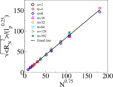
It is worth noting that the persistence length calculated from Eqn. 5 using the formula from WLC model uses the local correlation, namely the angle between the subsequent bond vectors and hence is expected to provide a decent value of the persistence length when EV is also included. The excellent collapse of the data for $\tilde{R}_{N}\sim N^{0.75}$ for various values of the stiffness parameter ($\kappa=1-192$) on the same master curve indicates that Eqn. 5 can be used as the standard definition of persistence length even in presence of the EV effect.

V.1.3 Comparison with WLC in 2d

Having established the definition of persistence length which validated Eqn. 20, we now use Eqn. 3 presented in section II to analyze the BD simulation results for the end-to-end distance. Please note that limiting cases of Eqn. 3 are either a Gaussian coil ($\langle R_{N}^{2}\rangle=2\ell_{p}L$ for $L\gg\ell_{p}$) or a rod ($\langle R_{N}^{2}\rangle=L^{2}$ for $L\ll\ell_{p}$). We have used simulation results to plot $\frac{\langle R_{N}^{2}\rangle}{2\ell_{p}L}\sim L/\ell_{p}$ for a large number of values($\sim 100$) of $L/\ell_{p}$ ($0.05\leq L/\ell_{p}\leq 170$).

Figure 4: $\langle\langle R_{N}^{2}\rangle/(2L\ell_{p})$ as a function of $L/\ell_{p}$ obtained from different combinations of chain length $N$ and stiffness parameter $\kappa$ (log-log scale). The solid (maroon) line is a fit to the formula $\langle R_{N}^{2}\rangle/2L\ell_{p}\sim(L/\ell_{p})^{0.5}$ for $4<L/\ell_{p}<170$. The inset shows the same for small values of $0<L/\ell_{p}<1$ which clearly indicates that limiting slope of unity ($\langle R_{N}^{2}\rangle=L^{2}$) for $L/\ell_{p}\rightarrow 0$.

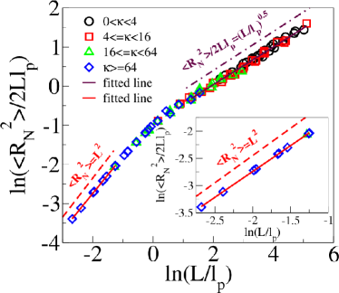
We have also taken additional care that a given value of $L/\ell_{p}$ is generated for different combinations of $L$ and $\ell_{p}$. These results are shown in Fig. 4. For $L/\ell_{p}\ll 1$ we observe that $\frac{\langle R_{N}^{2}\rangle}{2\ell_{p}L}\sim(L/\ell_{p})^{0.95}$ while for $L/\ell_{p}\gg 1$ the data very nicely fit with $\frac{\langle R_{N}^{2}\rangle}{2\ell_{p}L}\sim(L/\ell_{p})^{0.50}$. This is consistent with prior MC results using a lattice model by Hsu et al. Hsu_EPL_2011 . However, since our studies are done in continuum we are able to get data that is for much shorter length scales. The fact that in the rod-like regime ($L<\ell_{p}$) the “best fit” exponent is 0.95 rather than the asymptotic value 1.0 is due to the fact that for $\kappa$=32 and 64 the “rods” still exhibit nonnegligible transverse fluctuation unlike truly stiff rods. The Gaussian behavior that Eqn. 3 implies $\langle R_{N}^{2}\rangle/2L\ell_{p}=1$ for large $L$ would mean a horizontal straight line in Fig. 4, but no indication of such a behavior is seen. The simulation data then implies the strict absence of a Gaussian limit for 2d swollen semi-flexible chains due to severe dominance of the EV interaction. This result should be contrasted with the simulation results in 3d, where one sees a gradual crossover from rod limit to the EV limit (in 3d) passing through a Gaussian regime Moon_1991 ; Hsu_EPL_2010 .

V.1.4 Transverse Fluctuations

It is reasonable to define an average axis for a polymer chain in the rod limit ($\ell_{p}\gg L$). In this limit using WLC chain Hamiltonian the transverse fluctuation with respect to this average axis has been shown Fuji ; Odijk ; Capsi to obey the following equation

$$\langle l_{\bot}^{2}\rangle\sim L^{3}/\ell_{p},.$$ (21)

The above equation implies that the roughness exponent Barabasi $\zeta=3/2$ ($\sqrt{\langle l_{\bot}^{2}\rangle}\sim L^{\zeta}$) for a weakly bending rod. Starting from an extremely stiff chain where the transverse fluctuations are expected to be governed by the roughening exponent $\zeta=3/2$, if we approach the limit of fully flexible chain, then the fluctuations become isotropic and in this limit one can expect that $\langle l_{\bot}^{2}\rangle\sim L^{\nu}$, so that in 2d $\langle l_{\bot}^{2}\rangle\sim L^{0.75}$. In order to calculate the transverse fluctuation, in our simulation, for each configuration of the polymer chain, we choose $\hat{x}=\vec{R}_{N}/R_{N}$ as the longitudinal axis and calculate transverse fluctuations as follows:

$$\langle l_{\bot}^{2}\rangle=\frac{1}{N}\sum_{i=1}^{N}y_{i}^{2},$$ (22)

where $y_{i}$ is the perpendicular distance of the $i^{th}$ monomer with respect to the instantaneous direction $\vec{R}_{N}$. We have repeated this calculation for several chain lengths from extremely stiff chains to fully flexible chains.

Figure 5: (a) Log-log plot of $\sqrt{\langle l_{\bot}^{2}\rangle\ell_{p}}$ as a function of the contour length $L$ for chains of chain length $N=16$ (circle), 32 (square), 48 (diamond), 64 (up triangle), 96 (left triangle), 128 (down triangle), 256 (right triangle), 512($\times$) with various bending stiffness $\kappa=2$ (yellow), 4 (orange), 8 (magenta), 16 (brown), 32 (black), 48 (green), 64 (blue), 96 (indigo), 128 (cyan), 192 (red), 320 (dark green). The orange, magenta, brown, black solid lines are fitted to chains with $\kappa=4,8,16,32$, respectively. The maroon solid line is fitted for chains with $\ell_{p}>L/2$. (b) Log-log plot of $\sqrt{\langle l_{\bot}^{2}\rangle}/L$ as a function of $L/\ell_{p}$ showing excellent data collapse as well as maxima of the rescaled fluctuations around corresponding rescaled length $L/\ell_{p}\approx 1$.

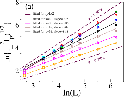
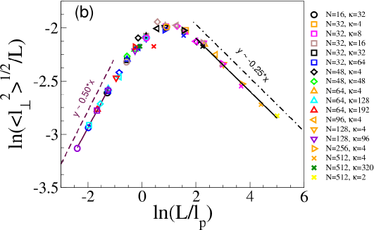
This is shown in Fig. 5(a). If one does not analyze the data carefully, one might be misled to conclude that the exponent $\zeta$ increases gradually with the chain stiffness $\kappa$. However, as we will see that the proper interpretation requires a scaling description in terms of $L/\ell_{p}$ as scaling variable. The interesting aspect of this rescaled dimensionless transverse fluctuation is shown in Fig. 5(b) as a function of rescaled length $L/\ell_{p}$ where the rescaled fluctuations collapse on the same master curve. This plot exhibits a maximum and then decreases gradually for large value of $L/\ell_{p}$. It is worth noting that analytical results do not exist for chains with intermediate stiffness. The physical origin of this maximum can be interpreted as follows. Starting from the stiff chain limit when $L/\ell_{p}\ll 1$ it increases for a more flexible chain when the chain undergoes shape changes from rod to ellipsoid-like blob, and finally to isotropic spherical blobs. Naturally, when chain flexibility is defined in units of the persistence length for some value of $L/\ell_{p}$ ($L/\ell_{p}\sim$ 3 from Fig. 5(b)) the fluctuation becomes maximum before it becomes isotropic. To the best of our knowledge this result is new and in principle can be used to measure the persistence length of a semiflexible polymer by measuring the transverse fluctuations using fluorescence probes. This would require numerically analyzing a large number of images of semiflexible chains (of a given kind of polymer) with varying contour length. For each image of a chain one can extract $L$ as well as the end-to-end vector $\vec{R}_{N}$ and then use Eqn. 22 to extract $\langle l_{\bot}^{2}\rangle$. Plotting then $\sqrt{\langle l_{\bot}^{2}\rangle}/L$ versus $L$ one would find $l_{p}$ from the position of the maximum of this plot.

V.1.5 Bond vector correlation

The orientational correlation between successive bonds decays exponentially in a WLC model according to Eqn. 4. However, recent Monte Carlo (MC) studies by Hsu, Paul, and Binder have verified that a swollen semiflexible chain in 2d exhibits a power law decay as a function of the separation $s$ between the beads Hsu_EPL_2011 given by

$$\left<\hat{b}_{i}\cdot\hat{b}_{i+s}\right>\propto s^{-\beta},\;\beta=2-2\nu\;\;{\rm for}\;s\ll N.$$ (23)

For a fully flexible chain $\nu=0.75$ in 2d so that $\beta=0.5$. It is then expected that a semiflexible chain will exhibit the same behavior when $L/\ell_{p}\gg 1$. While for very stiff chain one needs to have extremely long chain to see this asymptotic regime for large $L/\ell_{p}\gg 1$, yet satisfying the condition $s\ll N$, from our simulation we clearly see this trend for moderate values of $\kappa$.

We calculated the bond correlation function from its definition and tested both Eqn. 4 and 23. First in Fig. 6 we show the semi-log plot of Eqn. 4.

Figure 6: Semi-log plot. $\ell_{p}$ is calculated from the slope of the fitted line, which is very close to the values (correspondingly 105.8, 52.6, 25.9, 12.6, 6.05, 3.31) from $\ell_{p}=-1/\mathrm{ln}\langle\mathrm{cos}(\theta)\rangle$ (see Table 1).

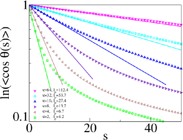
The straight lines are fitted only with the first several data points in order to get values of $\ell_{p}$ which are close to those calculated from $\ell_{p}=-1/\mathrm{ln}\langle\mathrm{cos}(\theta)\rangle$. The deviation from the initial slope (only after few points) clearly shows that Eqn. 4 predicted by the WLC model does not hold good for a 2d swollen chain as expected from the result of Fig. 4.

Fig. 7 shows the log-log plot of Eqn. 23 where we have also included the graph for a fully flexible chain for reference.

Figure 7: (a) Log-log plot of $\langle\cos\theta(s)\rangle$ as a function of $s$ for various combinations of $N$ and $\kappa$. While for large $\kappa$ the asymptotic slope of $s^{-0.5}$ is preempted by finite size effect, for $(N,\kappa)\equiv(1024,2)$ and $(N,\kappa)\equiv(2024,4)$ the slope of $-0.5$ is clearly visible; (b) Same as in (a) but using rescaled variable $s/\ell_{p}$ which shows excellent data collapse for $s/\ell_{p}\leq 1$. The inset shows the same but only for the cases to emphasize that in the limit $L/\ell_{p}\gg 1.0$ there is a perfect data collapse for the power law scaling.

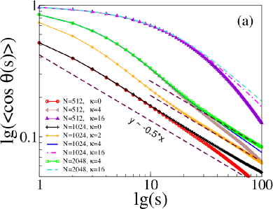
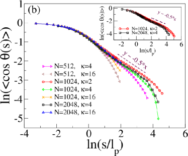
Please note that even for a fully flexible chain it requires a rather long chain length ($N=1024$) to clearly see the regime with slope with $\beta=0.5$ over an appreciably broad range of abscissa values. For comparison we put the graph for a shorter fully flexible chain of $N=512$. Here the curve starts to decrease faster before it reaches the slope corresponding to $\beta=0.5$. Naturally for stiffer chains (which could be thought of a flexible chain of length $L/\ell_{p}$ for this purpose) for the maximum chain length $N=2048$ considered in this paper we only see the regime characterized by $\beta=0.5$ only for $\kappa=2.0$ and 4.0.

It is expected that the bond vector correlation also exhibits a scaling behavior when studied as a function of $s/\ell_{p}$, as even for moderate values of $\ell_{p}\sim 5$ (see Fig. 6), this length rescaling $L\rightarrow L/\ell_{p}$ overrides the exponential decay for small $s/\ell_{p}$. With a choice of distance between monomers in units of $\ell_{p}$ all chains are expected to behave as fully flexible chains. Therefore, if we use the renormalized distance $s/\ell_{p}$ to replot Fig 7(a) then one expects that the power law correlation for chains with different stiffness will collapse on the same master plot. This is shown in Fig. 7(b). We observe excellent data collapse for $s/\ell_{p}\leq 1$. Deviations from this collapse occur at a progressively larger value of $s/\ell_{p}$ as the ratio $L/\ell_{p}$ increases either by increasing the contour length $L$ for a fixed $\ell_{p}$ or for the same contour length $L$ and lowering the value of $\ell_{p}$. This is expected, since Eqn. 23 can hold only for $s\ll N$. Of course, a numerical study of the regime $\ell_{p}/\langle b\rangle\ll s\ll N$ for large $\ell_{p}$ is prohibitively difficult. However, the inset shows both the data collapse and the $\beta=0.5$ regimes for two chain lengths ($N=1024$ and 2048) and for two values of $\kappa$ ($\kappa=2$ and $\kappa=4$) which proves beyond doubt that for $1\ll s/\ell_{p}\ll L/\ell_{p}$ the bond autocorrelation exhibits a power law decay of a fully flexible chain.

V.1.6 Radial distribution function for end-to-end distance

Figure 8: Comparison of the radial distribution for Eqn. 25 and the simulation for N=128 and 256 with various values of $\kappa$.

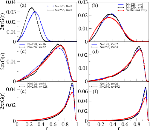
The Hamiltonian for the WLC chain model has been studied by many analytic technics assuming that for moderate chain lengths and stiff enough chains the EV effect will not dominate. Since we already established the severe dominance of the EV effect, Gaussian regime is absent for a 2d swollen chain. Here we compare the radial distribution functions for chains with different stiffness. In particular, we compare the results from our simulation with analytic results of Wilhelm and Frey Wilhelm_PRL_1996 in 2d. For the WLC model Wilhelm and Frey Wilhelm_PRL_1996 have derived expressions for the radial distribution functions $G(r)$ (both in 2d and 3d) in terms of infinite series. In 2d the expression for $G(r)$ is given as follows.

$$G(r)=\mathrm{const}\times t\sum^{\infty}_{l=0}\frac{(2l-1)\,!!}{2^{l}l\,!}\left[\frac{1}{2t(1-r)}\right]^{5/4}\times$$

$$\mathrm{exp}\left[-\frac{(l+1/4)^{2}}{2t(1-r)}\right]D_{3/2}\left[\frac{2l+1/2}{\sqrt{2t(1-r)}}\right],$$ (24)

where $t=\ell_{p}/L$, $r=R_{N}/L$ and $D_{3/2}(x)$ is a parabolic cylinder function. For the whole range of values of $\kappa$ in our simulation, when we plot the analytic result of Eqn. 24 we find that this series is fully dominated by the first term and we didn’t see visual differences from the plot that includes the first four terms. Therefore, in Fig. 8 we plot only the first term of this series ($l=0$) term given by

$$G_{l=0}(r)=\mathrm{const}\times t\times\left[\frac{1}{2t(1-r)}\right]^{5/4}\times$$

$$\mathrm{exp}\left[-\frac{(1/4)^{2}}{2t(1-r)}\right]D_{3/2}\left[\frac{1/2}{\sqrt{2t(1-r)}}\right]$$ (25)

Please note that for the radial distribution function Wilhelm and Frey Wilhelm_PRL_1996 does not take into account excluded volume effects. In Fig. 8 we have also included the distribution for a completely flexible chain ($\kappa=0$) for comparison purposes. For $\kappa=4$ and 8 (i.e., $L/\ell_{p}\approx 16$) the simulated distribution still is intermediate between the behavior of fully flexible chains (which we expect to result for $N\rightarrow\infty$ for all $\kappa$!) and the distribution of the Kratky-Porod model.

V.2 Dynamics

We now look at the dynamics of a swollen semi-flexible chain. We are using a Brownian dynamics (BD) scheme and therefore, HD effects are not included in our studies. However, for polymers adsorbed on a flat surface simulation studies have shown that the HD effects are negligible for no-slip boundary conditions Winkler . Thus we expect the results are relevant for a fair comparison of experimental studies. Also we would like to point out that unlike equilibrium properties, computational time increases dramatically to study time dependent properties for the same chain length. Thus the diffusion and relaxation studies for the longest chain length reported in this paper took significant time for well converged runs. We verified that the diffusion constant $D$ is independent of the persistence length $\ell_{p}$ and depends only on the chain length $N$ and scales as $D\sim k_{B}T/N$ with very good accuracy, as expected in a BD formalism.

Next we consider monomer relaxation dynamics of the chain. Following previous work for the relaxation of a fully flexible chain  Grest_Kremer_PRA_1986 ; Gerroff_JCP_1992 ; Milchev_JCP_1993 ; Binder_Review we have monitored various quantities pertaining to a single monomer relaxation. These quantities have been studied in the past using BD algorithm Grest_Kremer_PRA_1986 , and dynamical Monte Carlo algorithms (DMC) Gerroff_JCP_1992 ; Milchev_JCP_1993 , including the bond-fluctuation model (BFM) Binder_Review . The dynamics of the individual monomers and the collective dynamics for the whole chain have been characterized by the functions $g_{1}(t)$, $g_{2}(t)$, $g_{3}(t)$, $g_{4}(t)$, and $g_{5}(t)$. They are defined as follows:

$$g_{1}(t)=\langle\left[\mathbf{r}_{N/2}(t)-\mathbf{r}_{N/2}(0)\right]^{2}\rangle,$$ (26a)

$$g_{2}(t)=$$

$$\langle\left[\left(\mathbf{r}_{N/2}(t)-\mathbf{r}_{CM}(t)\right)-\left(\mathbf{r}_{N/2}(0)-\mathbf{r}_{CM}(0)\right)\right]^{2}\rangle,$$ (26b)

$$g_{3}(t)=\langle\left[\mathbf{r}_{CM}(t)-\mathbf{r}_{CM}(0)\right]^{2}\rangle,$$ (26c)

$$g_{4}(t)=\langle\left[\mathbf{r}_{end}(t)-\mathbf{r}_{end}(0)\right]^{2}\rangle,$$ (26d)

$$g_{5}(t)=$$

$$\langle\left[\left(\mathbf{r}_{end}(t)-\mathbf{r}_{CM}(t)\right)-\left(\mathbf{r}_{end}(0)-\mathbf{r}_{CM}(0)\right)\right]^{2}\rangle.$$ (26e)

The quantities $g_{1}(t)$, $g_{3}(t)$, and $g_{4}(t)$ reflect the time dependence of the position of the middle monomer, the center of mass, and the end monomer of the chain respectively. At late times for distances greater than the gyration radius the functions $g_{1}(t)$, $g_{3}(t)$ and $g_{4}(t)$ will describe the motion of the entire chain. Consequently,

$$g_{1}(\tau(N,\ell_{p}))\sim g_{3}(\tau(N,\ell_{p})\sim g_{4}(\tau(N,\ell_{p})\sim t,$$ (27)

for $t\geq\tau_{2}(N,\ell_{p})$ where $\tau_{2}$ is given by Eqn. 12. The quantities $g_{2}(t)$ and $g_{5}(t)$ on the contrary measure the relative displacement of the middle and the end monomer with respect to the center of mass of the chain. The functions $g_{2}(t)$ and $g_{5}(t)$ saturate at finite static values $2\langle\left(\vec{r}_{N/2}-\vec{r}_{CM}\right)^{2}\rangle$ and $2\langle\left(\vec{r}_{end}-\vec{r}_{CM}\right)^{2}\rangle$ respectively, since for $t\rightarrow\infty$ the orientations of the vectors $\vec{r}_{N/2}(t)-\vec{r}_{CM}(t)$, $\vec{r}_{end}(t)-\vec{r}_{CM}(t)$ are uncorrelated with their counterparts at $t=0$.

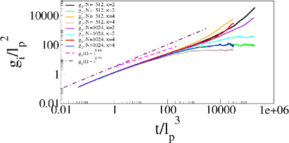
To study monomer dynamics, we have carried out BD simulation for various chain lengths $N=64-1024$ and for chain stiffness $\kappa=0-64$. We only show a limited set of data. As a reference and for comparison with the data for chains with $\kappa\neq 0$, we first show data for a fully flexible chain where we expect to see a single crossover dynamics from $g_{1}(t)\sim t^{0.6}$ at an early time for $0<t<\tau_{2}$ to a purely diffusive dynamics for the entire chain ($g_{1}(t)\sim t$). This is shown in Fig. 9 for chain length $N=512$ and 1024 respectively.

Figure 9: (a) $g_{i}(t)\sim t$ ($i=1-5$) for a fully flexible chain ($\kappa=0.0$) of length $N=512$. (b) $g_{i}(t)\sim t$ ($i=1-3$) for a fully flexible chain of length $N=1024$.

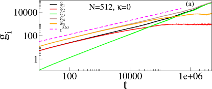
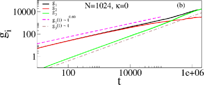
We have checked that the graphs for other chain length are similar and have the $t^{0.6}$ dependence for the fully flexible chain. At late times the functions $g_{2}$ and $g_{5}$ saturates and the functions $g_{1}$, $g_{3}$ and $g_{4}$ grow linearly as a function of time, becoming practically indistinguishable from each other. Similar studies have been reported earlier by Grest and Kremer Grest_Kremer_PRA_1986 and by Gerroff, Milchev, Paul, and Binder Gerroff_JCP_1992 ; Milchev_JCP_1993 ; Binder_Review . However, our studies are much more exhaustive and quantitatively captures the crossover from $t^{0.6}$ to the purely diffusive regime which were only qualitative in previous studies and for shorter chains.

We now show data for the double crossover to support our scaling analysis for $\kappa\neq 0$. In particular we show data for chain length $N=512$ with $\kappa=$2.0 and $N=1024$ with $\kappa=$2.0, 4.0 respectively. Unlike Fig. 9 for $\kappa=0$, plots for $g_{1}(t)$, $g_{2}(t)$ shown in Fig. 10 are characterized by a $t^{0.75}$ slope which then crosses over to the regime characterized by $g_{1}(t)\sim g_{2}(t)\sim t^{0.6}$ and that $g_{1}(t)$ eventually merges with $g_{3}(t)$. When we compare Fig. 10(a) and Fig. 10(b) consistent with the prediction of scaling theory we observe that the extent of the $t^{0.75}$ region in both the graphs are the same as they have the same value of $\kappa=2$, although the chain lengths are different. Likewise, comparing Fig. 10(b) and Fig. 10(c) we note that since both plots have the same chain length the beginning of the second crossover occur almost at the same time ($\tau_{2}\propto N^{2.5}$) but since the latter chain is twice as stiff it has a wider $t^{0.75}$ regime resulting in a narrower span of $t^{0.6}$ regime. Thus Fig. 10 unambiguously confirms predictions from the scaling theory. We observe that at early time $g_{1}(t)=g_{2}(t)$; however the width of the region $g_{2}(t)\sim t^{0.6}$ is narrower than that of $g_{1}(t)\sim t^{0.6}$ and it exhibits a slightly lower value of slope before saturation. Considering that the crossovers are broad, we believe that this is due to finite size effect as it is evident if we compare Fig. 10(a) and Fig. 10(b). In the latter case, which is for a larger chain length, the difference between $g_{1}(t)$ and $g_{2}(t)$ are much smaller and we notice that the difference begins at a later time. Ideally for very large system the point when $g_{1}(t)$ would change its slope towards $g_{1}(t)\sim t$, $g_{2}(t)$ also tend to saturate. The sharpness of this feature would require a much larger system. We also note the same feature in Fig. 9.

Figure 10: (a) Plot for $g_{1}(t)$ (black), $g_{2}(t)$ (red) and $g_{3}(t)$ (green) as a function of time on a log-log scale for chain length $N=512$ and $\kappa=2.0$. The blue and magenta dashed lines correspond to straight lines $g_{1}(t)=At^{0.75}$, and $g_{1}(t)=Bt^{0.60}$, respectively, where $A$ and $B$ are constants. (b) same but for $N=1024$ and $\kappa=2.0$. (c) same but for $N=1024$ and $\kappa=4.0$. Note that for a fully flexible chain the slope of the curve $\mathrm{log}(g_{i})\;\mathrm{versus}\;\mathrm{log}(t)$ would monotonously increase with time, unlike the present case.

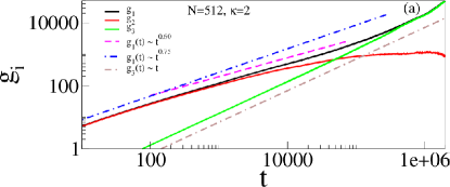
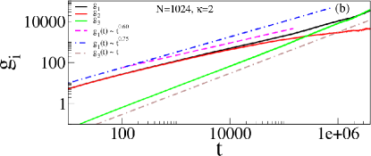
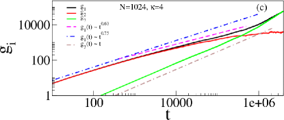
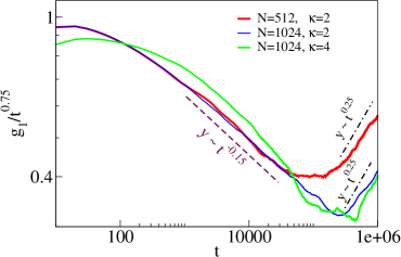
But the plots for $g_{1}(t)$ quite clearly show three distinct scaling regimes of $g_{1}(t)\sim t^{0.75}$ crossing over to $g_{1}(t)\sim t^{0.6}$ and then merging with $g_{3}(t)\sim t$ at late times. We have further confirmed the existence of this double crossover by plotting $g_{1}(t)/t^{0.75}\sim t$ as shown in Fig. 11. The existence of an initial plateau ($t<\tau_{1}$), followed by a decay ( $\propto t^{-0.15}$), and of a minimum (near $\tau_{2}$) before the diffusion ($\propto t^{0.25}$) starts further demonstrates quite conclusively that the exponent changes from $t^{0.75}\rightarrow t^{0.6}\rightarrow t$. We would like to mention that because of the width of the $t^{0.6}$ regime becomes narrower for stiffer chains we were unable to see this regime unambiguously in simulation of shorter chains and/or larger $\kappa$ (e.g., for $N=512$ and $\kappa\geq 4$ ). While for $N=512$ the double crossover is clear for $\kappa=2.0$, but becomes ambiguous for $\kappa\geq 4.0$ which required an increased chain length of $N=1024$. As expected, the crossovers are rather gradual, spread out over a decade in time $t$ each, and hence for chains that are not long enough the existence of these regimes is missed in previous work.

Figure 11: Log-log plot of $g_{1}(t)/t^{0.75}$ as a function of $t$ corresponding to the plots of Fig. 10(a) (red), (b) (blue) and (c) (green) respectively. In each graph the minimum occurs in the intermediate regime characterized by $t^{0.6}$.

The interplay of Rouse modes and the bending modes with respect to the monomer dynamics of semiflexible chains was considered in early work by Harnau et al. Harnau1 , in the framework of a Rouse model generalized by higher order terms to account for chain stiffness. They ignored excluded volume, and considered a single chain length, attempting to model $C_{100}$ alkanes in a melt. They found that their results were neither consistent with the Rouse behavior ($g_{1}(t)\sim t^{1/2}$) nor with the power law due to bending modes ($g_{1}(t)\sim t^{3/4}$ ). In our view, the chain length studied in this work was too small to observe both power laws separately, rather all their data fall in a regime of smooth crossover. Having established the double-crossover we now further investigate the consequence of scaling prediction that the first crossover occurs at time $\tau_{1}\propto\ell_{p}^{3}$ when $g_{1}(\tau_{1})\propto\ell_{p}^{2}$. Fig. 12 shows a plot of $g_{1}(t)/\ell_{p}^{2}$ as a function of rescaled time $t/\ell_{p}^{3}$ which shows data collapse for $g_{1}(t)/\ell_{p}^{2}\leq 1.0$ and $t/\ell_{p}^{3}\leq 1.0$ for various combinations of chain length $N$ and $\kappa$ confirming the length and the time scales for these crossovers. Note that the scaling theory of section III implies

$$g_{i}(t)/\ell_{p}^{2}=\tilde{g}(t/\tau_{1},t/\tau_{2}),$$ (28)

where $\tau_{1}$, $\tau_{2}$ are the times defined in Eqn. 8 and 12. If the first argument of the scaling function $\tilde{g}$, $t/\tau_{1}$ is small in comparison to unity, we can approximate Eqn. 28 as $g_{1}(t)/\ell_{p}^{2}\approx\tilde{g}(t/\tau_{1},0)\propto\left(t/\tau_{1}\right)^{3/4}$, which reduces to Eqn. 7. For $t/\tau_{1}>1$ we can rewrite the scaling function as

$$g_{i}(t)/\ell_{p}^{2}=\tilde{\tilde{g}}(t/\tau_{1},\tau_{2}/\tau_{1})=\tilde{\tilde{g}}(t/\tau_{1},\left(L/\ell_{p}\right)^{5/2}).$$ (29)

Note that $\tau_{2}/\tau_{1}$ remains constant when we increase $N$ and $\ell_{p}$ by the same factor: this observation explains that the scaling of the data in Fig. 12 encompasses the full range of times.

Figure 12: Plot for $g_{1}(t)/\ell_{p}^{2}$ and $g_{2}(t)/\ell_{p}^{2}$ as a function of $t/\ell_{p}^{3}$ on a log-log scale for chain lengths $N=512$, 1024 with $\kappa=2.0$, 4.0 respectively. The dot-dashed and dashed lines correspond to slopes 0.75 (maroon) and 0.6 (magenta) respectively.

VI Summary and Discussion

In conclusion, we have studied conformations, fluctuations, and crossover dynamics of a swollen semiflexible chain in 2d. We first developed a scaling theory which generalizes early time monomer dynamics of a fully flexible chain for a semiflexible chain characterized by its contour length and the persistence length. We predict a double crossover which arises due to the presence of an additional length scale introduced through the chain persistence length. Monomer dynamics up to a length scale $\ell_{p}$ is independent of chain length and is characterized by the $t^{0.75}$ power law. At a later time $t>\tau_{1}$ when the size of the fluctuations becomes bigger than $\ell_{p}$ the dynamics begin to look like that of a fully flexible chain and characterized by the well known $t^{2\nu/1+2\nu}$ growth. Both of these exponents have been discussed in the literature separately but have not been emphasized that before the entire chain reaches purely diffusive regime, there ought to be two and not one crossover, the first crossover differentiates chains of different stiffness. Previously the dynamics of monomer MSD of semiflexible polymers has also been studied by Harnau et al. Harnau1 , using a Rouse-type model generalized to include chain stiffness. They saw a gradual crossover, in between bending modes and Rouse modes, but did not consider the scaling description of the crossover. Note that excluded volume effects were absent in their model, and hence it is not applicable in $d=2$ dimensions.

Motivated by recent lattice MC results for a swollen chain in 2d predicting the absence of a Gaussian regime we undertook similar studies in 2d continuum using BD simulation. While checking our data for the RMS end-to-end distance for chain of different contour length and persistence length we discovered that we regain the well known results for the end-to-end distance due to Schaefer, Joanny, and Pincus Pincus_MM_1980 and Nakanishi Nakanishi_1987 provided we use the definition of the persistence length given by either the lattice or continuum version of the Kratky-Porod WLC model. We explain this by noting that the persistence length being a local property of a chain does not depend on the EV interaction. This is further reassured when we note that the persistence length calculated this way does not depend on the chain length unlike well used textbook definition of persistence length where the projection of the end-to-end vector on the first bond is used as the definition and does depend on the chain length. Therefore, we emphasize that the latter definition needs to be discarded.

We also confirm the absence of the Gaussian regime in the continuum bead-spring model where the swollen chain for $L/\ell_{p}\ll 1$ behaves like a rod and thereafter always behaves like a swollen chain. Considering that there are increased number of activities to explore the properties of biomolecules on a surface, our result (Fig. 4) will be extremely valuable to analyze the experimental data correctly for stiff molecules on flat surfaces. It has not escaped our attention that many such reported analyses are still done using the WLC model and/or calculating the chain persistence length from projected end-to-end to the first bond.

Transverse fluctuations in a stiff chain has been addressed analytically in the literature only in the extremely stiff chain limit where one finds that it is described by the roughening exponent. Analytic calculations for moderately stiff chains are hard to carry out, and to date there are no results for transverse fluctuations spanning the entire regime from a stiff to a fully flexible chain. We have numerically obtained this result and pointed out that the appropriate length variable to analyze the data is to use the persistence length as the unit of length. When we use $L/\ell_{p}$ as the length scale to plot transverse fluctuation we discover the non-monotonic behavior of this fluctuation reaching a maximum for some $L\gtrapprox\ell_{p}$. We point out that this universal scaling of the transverse fluctuation can be used to measure the persistence length of the chain. Another accompanying consequence of the absence of Gaussian regime for a swollen chain in 2d is the decay of the bond correlation function which exhibits a power law decay. Again, by choosing the normalized contour segment $s/\ell_{p}$ as the appropriate variable we regain the exponent $\beta=0.5$ which describes the decay of bond autocorrelation for a fully flexible chain. We must point out that many of these results and analyses on chain conformations and equilibrium fluctuations point to a common theme. In the limit $L/\ell_{p}\gg 1$ we recover the expected behavior of a fully flexible chain and chains with different stiffness exhibit universal scaling behavior when persistence length is chosen as the unit of length.

This general idea extends to our study of monomer dynamics as well. We have provided a new scaling theory of monomer dynamics for semiflexible polymers in 2d. Our theory predicts novel crossover dynamics at an intermediate time when the fluctuations of the monomers $g_{1}(\tau_{1})\sim\ell_{p}^{2}$. Around this time the monomer dynamics become the same as that of a fully flexible swollen chain characterized by $g_{1}(t)\sim t^{2\nu/(1+2\nu)}=t^{0.6}$ in 2d . The theory expands the existing scaling theory for monomer dynamics for a WLC and that of a fully flexible chain to include the effect of the chain persistence length. Fully flexible swollen chains are self-similar objects, while a polymer segment up to its own persistence length is not. Therefore, it is expected that for length scales up to $\ell_{p}$ the dynamics will have different characteristics due to bending modes arising out of the chain stiffness. The EV effect is almost negligible for the $t^{0.75}$ regime and therefore, our result is the same as that of previous studies using WLC Hamiltonian Granek_1997 ; Maggs_MM_1993 . For the $t^{0.6}$ regime originating from the EV effect, where the monomer dynamics are governed by Rouse relaxation of a fully flexible chain, our theory elucidates the exact role of chain persistence length neither contained in WLC model nor studied before. We also validate our new scaling theory by extensive BD simulation results.

A subtle issue concerns the limit $\kappa$ towards infinity while keeping the contour length $L$ fixed. Then transverse motions of the monomers relative to each other, in a coordinate system where the $x$-axis is fixed along the rod-like polymer, are completely suppressed. In the “laboratory coordinate system”, however, the rod still can make random transverse motions, namely rigid body rotations and translations. However, in addition to those motions still motions of the monomers relative to each other along the axis of the rod are possible. These motions may give rise to a transient $t^{1/2}$ behavior, as a model calculation for a one-dimensional harmonic chain shows huang_1d . However, our data for $g_{i}(t)$ for large $\kappa$ due to the smoothness of crossovers did not allow to clearly separate this mode of motions from the displacements due to transverse fluctuations.

In the present manuscript we have ignored HD interactions as they are not significant for 2d swollen chains on a substrate. However we now present simple estimates of generalization of our results in 3d and/or in presence of HD interactions which will be relevant for a 3d swollen chain. In the free draining limit, the results $t^{0.75}$ will remain the same in 3d Granek_1997 ; Maggs_MM_1993 , but the intermediate Rouse relaxation regime will be characterized by $t^{2\nu/(1+2\nu)}=t^{0.54}$ ($\nu=0.59$ in 3d), for the case where the EV is relevant (i.e., MSDs exceeding $R^{\ast 2}=\ell_{p}^{2}/b^{2}$). For MSD in between $\ell_{p}^{2}$ and $R^{\ast 2}$ Gaussian behavior prevails, $\nu=1/2$, and hence $g_{1}(t)\propto t^{1/2}$ in that regime. The crossover between flexible and stiff chain dynamics in 3d in the free draining limit was studied by Steinhauser et al. Steinhauser , but no scaling analysis is done.

Replacing Rouse relaxation by Zimm relaxation one immediately sees that in presence of HD interaction the intermediate regime is characterized by $t^{2\nu/3\nu}=t^{2/3}$ Hinczewski ; Netz_EPL_2009 ; Hinczewski_PhysicaA . Notice that in this case $\nu$ cancels out and this relaxation should be the same in 2d and 3d. However, as shown by Hinczewski and Netz  Netz_EPL_2009 ; Hinczewski_PhysicaA , very complicated crossovers occur in this case.

We now make some comments about some recent experiments to study monomer dynamics. This is typically done using FCS where a tagged monomer can be directly watched in real time. However, as has been mentioned by Petrov et al. Petrov that since the $t^{0.75}$ regime or the intermediate regimes (either $t^{0.5}$ or $t^{2/3}$) occur at much shorter time scales compared to the longest relaxation time, unless extreme caution is taken for the measurement of MSD of a labeled particle, the interpretation can be misleading, especially for shorter DNA fragments Shusterman_PRL_2004 . For dsDNA of length $10^{2}-2\times 10^{4}$ base pairs (which is equivalent to $L/\ell_{p}\sim 0.7-140)$ fluorescence correlation spectroscopy (FCS) studies of Petrov et al. observed the Zimm regime characterized by a $t^{2/3}$ power law. However, a clear demonstration of the double crossover is lacking in recent experiments with biopolymers Sackmann_NJP ; Goff_PRL_2002 ; Capsi ; Shusterman_PRL_2004 ; Petrov . This is partly due to lack of resolution of the experiments and partly due to the fact that lacking any theoretical predictions for this phenomenon, researchers did not specifically investigate the precise behavior of MSD before the onset of overall chain diffusion very carefully. We will provide some physical arguments why the experimental detection can be hard: a simple calculation for Fig. 1 shows that in order for the width of the $t^{0.75}$ and $t^{0.60}$ to be equal (in logarithmic scale) one needs $N=\ell_{p}^{2.2}$ in 2d. In other words for a stiffer chain one needs a very long chain to see the $t^{0.60}$ regime. Indeed in our simulation we found (not shown here) that for $\kappa=16$, 32, and 64, the results with chain length up to $N=512$ are largely dominated by the $t^{0.75}$ regime and we did not clearly see the $t^{0.60}$ regime. It is only after we lowered the value of $\kappa$ and used longer chain ($N=1024$), we identified these two regimes quite conclusively (Fig. 10). We suspect that the same might happen in experiments Sackmann_NJP . For extremely stiff chains the $t^{0.6}$ (or $t^{0.54}$ in 3D) region can be extremely narrow and could either be missed or the rather smooth double crossover might be mistakenly interpreted as a single crossover (with $t^{2/3}$ in 2d). Therefore, we believe that these results will not only promote new experiments but will be extremely valuable in identifying and interpreting different scaling regimes for the monomer dynamics of semiflexible polymers.