On Neutrino Masses in the MSSM with

BRpV


Marco A. Díaza, Maximiliano A. Riverab and Nicolás Rojasa


aDepartamento de Física, Universidad Católica de Chile,

Avenida Vicuña Mackenna 4860, Santiago, Chile

bDepartamento de Física, Universidad Técnica Federico Santa María

Casilla 110-V, Valparaiso, Chile

mad@susy.fis.puc.cl, maximiliano.rivera@usm.cl, nrojas1@uc.cl


Abstract

One loop corrections to the neutrino mass matrix within the MSSM with Bilinear R Parity Violation are calculated, paying attention to the approach in which an effective 3×3333\times 3 neutrino mass matrix is used. The full mass matrix is block diagonalized, it is found that second and third order terms can be numerically important, and this is analytically understood. Top-stop loops do not contribute to the effective 3×3333\times 3 at first order, nevertheless they contribute at third. An improved 3×3333\times 3 approach that include these effects is proposed. A scan over parameter space is made supporting the conclusions.

1 Introduction

The evidence for neutrino oscillation comes from many experiments around the world [1, 2, 3, 4, 5, 6, 7, 8, 9]. The activity around neutrino physics has grown due to a more precise determination of neutrino oscillation parameters, specially coming from experiments connected with the reactor angle θ13subscript𝜃13\theta_{13} [10, 11, 12, 13, 14]. Global fits [15] using data from the mentioned experiments, allow to extract three mixing angles: two large θ21subscript𝜃21\theta_{21} and θ23subscript𝜃23\theta_{23}, one small θ13subscript𝜃13\theta_{13}, and two mass scales Δm212Δsubscriptsuperscript𝑚221\Delta m^{2}_{21} and Δm322Δsubscriptsuperscript𝑚232\Delta m^{2}_{32}. This information, constitutes an experimental evidence that the Standard Model (SM) must be extended.

If neutrinos are massive Majorana particles, lepton number violating terms must be present. In the Minimal Supersymmetric Standard Model (MSSM) [16] with Bilinear R-Parity Violation (BRpV) [17], R-parity is broken via lepton number violation, introducing a bilinear term at the superpotential level [18, 19, 20, 21]. Therefore, neutrino masses and mixing angles are generated via a low-energy see-saw mechanism, mixing neutrino flavor-eigenstates and neutralinos. Although this solution is appealing to explain neutrino masses and mixing angles, signals for supersymmetry at the LHC have not been seen [22]. Since the majority of the searches are based on supersymmetry with bilinear R-parity conserved, there is an open window for it.

In the MSSM with R-Parity violation, one neutrino mass is generated at tree-level, while the other two neutrinos remain massless. To reconcile theoretical predictions with the experimental data requires going beyond the tree-level approximation [23]. Several authors have shown the dependence of the neutrino masses in terms of the parameter which bilinearly violate R-parity, and also how to determine these from collider physics [24]. Improvements in the precision measurement of the neutrino parameters [25], as it will be discussed, suggest to go beyond one loop order in the calculation of the neutrino masses.

The most convenient way to numerically introduce one loop corrections to neutrino masses in this model is through the 7×7777\times 7 mass matrix, which includes 4 neutralinos and 3 neutrinos. If this mass matrix is block diagonalized, an effective 3×3333\times 3 neutrino mass matrix is generated, and it is very convenient when an algebraical understanding is sought. Nevertheless, the 3×3333\times 3 approach can miss important numerical effects. This motivates a more careful treatment of the block diagonalization, leading to an improved 3×3333\times 3 approach.

The paper is organized as follow: In section 2, introductory remarks about neutrino mass generation in BRpV are provided. Section 3 shows how loop corrections are treated in this article. Section 4 develops algebraic approximations that explain the numerical effects. Finally, conclusions about the findings are provided.

2 Neutrino Masses in Bilinear R-Parity Violation

Models with BRpV include a bilinear term in the superpotential that violates simultaneously R-Parity and lepton number. The superpotential has the following form,

W=WYuk+εab(μH^daH^ub+ϵiL^iaH^ub),𝑊subscript𝑊𝑌𝑢𝑘subscript𝜀𝑎𝑏𝜇superscriptsubscript^𝐻𝑑𝑎superscriptsubscript^𝐻𝑢𝑏subscriptitalic-ϵ𝑖superscriptsubscript^𝐿𝑖𝑎superscriptsubscript^𝐻𝑢𝑏W=W_{Yuk}+\varepsilon_{ab}\left(-\mu\widehat{H}_{d}^{a}\widehat{H}_{u}^{b}+\epsilon_{i}\widehat{L}_{i}^{a}\widehat{H}_{u}^{b}\right), (2.1)

where in WYuksubscript𝑊𝑌𝑢𝑘W_{Yuk} one has the usual R-Parity conserving (hereafter, RpC) Yukawa terms. Here the explicit bilinear terms are shown, with μ𝜇\mu the higgsino mass and ϵisubscriptitalic-ϵ𝑖\epsilon_{i} the BRpV mass parameters. In this work trilinear R-Parity violating terms are not considered, motivated by models that generate BRpV and not TRpV [26]. The terms shown in eq. (2.1) induce a mixing between neutralinos and neutrinos, forming a set of seven neutral fermions Fi0subscriptsuperscript𝐹0𝑖F^{0}_{i}. The corresponding tree level mass terms can be written by a 7×7777\times 7 mass matrix as follows,

N0=[Mχ0mTm0].superscriptsubscript𝑁0delimited-[]superscriptsubscriptM𝜒0superscript𝑚𝑇𝑚0{\cal M}_{N}^{0}=\left[\begin{array}[]{cc}{\mathrm{M}}_{\chi}^{0}&m^{T}\\ m&0\end{array}\right]. (2.2)

The sub-matrix Mχ0superscriptsubscriptM𝜒0{\mathrm{M}}_{\chi}^{0} is the usual tree-level neutralino mass matrix of the MSSM, and m𝑚m is the BRpV mixing matrix which mix neutralinos and neutrinos. Those are given by,

Mχ0=[M1012gvd12gvu0M212gvd12gvu12gvd12gvd0μ12gvu12gvuμ0]superscriptsubscriptM𝜒0delimited-[]subscript𝑀1012superscript𝑔subscript𝑣𝑑12superscript𝑔subscript𝑣𝑢0subscript𝑀212𝑔subscript𝑣𝑑12𝑔subscript𝑣𝑢12superscript𝑔subscript𝑣𝑑12𝑔subscript𝑣𝑑0𝜇12superscript𝑔subscript𝑣𝑢12𝑔subscript𝑣𝑢𝜇0\displaystyle{\mathrm{M}}_{\chi}^{0}=\left[\begin{array}[]{cccc}M_{1}&0&-\frac{1}{2}g^{\prime}v_{d}&\frac{1}{2}g^{\prime}v_{u}\\ 0&M_{2}&\frac{1}{2}gv_{d}&-\frac{1}{2}gv_{u}\\ -\frac{1}{2}g^{\prime}v_{d}&\frac{1}{2}gv_{d}&0&-\mu\\ \frac{1}{2}g^{\prime}v_{u}&-\frac{1}{2}gv_{u}&-\mu&0\end{array}\right] ;absent\displaystyle\,\,\,;\,\,\,\, m=[12gv112gv10ϵ112gv212gv20ϵ212gv312gv30ϵ3].𝑚delimited-[]12superscript𝑔subscript𝑣112𝑔subscript𝑣10subscriptitalic-ϵ112superscript𝑔subscript𝑣212𝑔subscript𝑣20subscriptitalic-ϵ212superscript𝑔subscript𝑣312𝑔subscript𝑣30subscriptitalic-ϵ3\displaystyle m=\left[\begin{array}[]{cccc}-\frac{1}{2}g^{\prime}v_{1}&\frac{1}{2}gv_{1}&0&\epsilon_{1}\cr-\frac{1}{2}g^{\prime}v_{2}&\frac{1}{2}gv_{2}&0&\epsilon_{2}\cr-\frac{1}{2}g^{\prime}v_{3}&\frac{1}{2}gv_{3}&0&\epsilon_{3}\end{array}\right]. (2.10)

The matrix m𝑚m includes the sneutrino vacuum expectation values visubscript𝑣𝑖v_{i}. These vev‘s appear induced by the ϵisubscriptitalic-ϵ𝑖\epsilon_{i} in the superpotential as well as by the corresponding soft bilinear terms, not shown in this article (for more details, see [20, 27]). Eq. (2.2) can be block-diagonalized using the rotation matrix,

𝐑bd0=[112ξTξξTξ112ξξT],subscriptsuperscript𝐑0𝑏𝑑delimited-[]112superscript𝜉𝑇𝜉superscript𝜉𝑇𝜉112𝜉superscript𝜉𝑇{\bf R}^{0}_{bd}=\left[\begin{array}[]{cc}1-\frac{1}{2}\xi^{T}\xi&\xi^{T}\\ -\xi&1-\frac{1}{2}\xi\xi^{T}\end{array}\right], (2.11)

with ξ=mMχ01𝜉𝑚superscriptsuperscriptsubscriptM𝜒01\xi=m\,{{\mathrm{M}}_{\chi}^{0}}^{-1}. In this way, the block-diagonal mass matrix is,

Nbd,0superscriptsubscript𝑁𝑏𝑑0\displaystyle{\cal M}_{N}^{bd,0} =\displaystyle= [Mχ0+12(mTmMχ01+Mχ01mTm)00mMχ01mT]delimited-[]superscriptsubscriptM𝜒012superscript𝑚𝑇𝑚superscriptsuperscriptsubscriptM𝜒01superscriptsuperscriptsubscriptM𝜒01superscript𝑚𝑇𝑚00𝑚superscriptsuperscriptsubscriptM𝜒01superscript𝑚𝑇\displaystyle\left[\begin{array}[]{cc}{\mathrm{M}}_{\chi}^{0}+\frac{1}{2}(m^{T}m\,{{\mathrm{M}}_{\chi}^{0}}^{-1}+{{\mathrm{M}}_{\chi}^{0}}^{-1}m^{T}m)&0\\ 0&-m\,{{\mathrm{M}}_{\chi}^{0}}^{-1}\,m^{T}\end{array}\right] (2.14)
\displaystyle\equiv [Mχbd,000Mνbd,0].delimited-[]matrixsuperscriptsubscriptM𝜒𝑏𝑑000superscriptsubscriptM𝜈𝑏𝑑0\displaystyle\left[\begin{matrix}{\mathrm{M}}_{\chi}^{bd,0}&0\cr 0&{\mathrm{M}}_{\nu}^{bd,0}\end{matrix}\right]. (2.15)

The correction in the neutralino sector is usually ignored, while the correction in the neutrino sector is the well known tree-level neutrino effective mass matrix,

𝐌νbd,0=mMχ01mT=M1g2+M2g24detMχ0[Λ12Λ1Λ2Λ1Λ3Λ2Λ1Λ22Λ2Λ3Λ3Λ1Λ3Λ2Λ32],subscriptsuperscript𝐌𝑏𝑑0𝜈𝑚superscriptsuperscriptsubscriptM𝜒01superscript𝑚𝑇subscript𝑀1superscript𝑔2subscript𝑀2superscript𝑔24superscriptsubscriptM𝜒0delimited-[]superscriptsubscriptΛ12subscriptΛ1subscriptΛ2subscriptΛ1subscriptΛ3missing-subexpressionsubscriptΛ2subscriptΛ1superscriptsubscriptΛ22subscriptΛ2subscriptΛ3missing-subexpressionsubscriptΛ3subscriptΛ1subscriptΛ3subscriptΛ2superscriptsubscriptΛ32missing-subexpression{\bf M}^{bd,0}_{\nu}=-m\,{{\mathrm{M}}_{\chi}^{0}}^{-1}\,m^{T}=\frac{M_{1}g^{2}+M_{2}g^{\prime 2}}{4\det{{\mathrm{M}}_{\chi}^{0}}}\left[\begin{array}[]{cccc}\Lambda_{1}^{2}&\Lambda_{1}\Lambda_{2}&\Lambda_{1}\Lambda_{3}\cr\Lambda_{2}\Lambda_{1}&\Lambda_{2}^{2}&\Lambda_{2}\Lambda_{3}\cr\Lambda_{3}\Lambda_{1}&\Lambda_{3}\Lambda_{2}&\Lambda_{3}^{2}\end{array}\right], (2.16)

with Λi=μvi+ϵivdsubscriptΛ𝑖𝜇subscript𝑣𝑖subscriptitalic-ϵ𝑖subscript𝑣𝑑\Lambda_{i}=\mu v_{i}+\epsilon_{i}v_{d}. The matrix clearly has only one eigenvalue different from zero, which is experimentally unacceptable.

It is known that this problem is solved by radiative corrections. Concentrating only on loops with neutrinos in the external legs, one has for example,

νjsubscript𝜈𝑗\nu_{j}S0subscriptsuperscript𝑆0S^{0}_{\ell}Fk0subscriptsuperscript𝐹0𝑘F^{0}_{k}νisubscript𝜈𝑖\nu_{i}

where Fk0subscriptsuperscript𝐹0𝑘F^{0}_{k} are the mentioned neutral fermions and S0subscriptsuperscript𝑆0S^{0}_{\ell} are scalars formed by the mixing between Higgs bosons and sneutrinos [20]. These contributions can be calculated approximately in the block-diagonalized basis, obtaining a generalization to the neutrino mass matrix in eq. (2.16), which is customary to write as,

[𝐌νbd(1)]ij=AΛiΛj+B(Λiϵj+Λjϵi)+Cϵiϵj,subscriptdelimited-[]subscriptsuperscript𝐌𝑏𝑑1𝜈𝑖𝑗𝐴subscriptΛ𝑖subscriptΛ𝑗𝐵subscriptΛ𝑖subscriptitalic-ϵ𝑗subscriptΛ𝑗subscriptitalic-ϵ𝑖𝐶subscriptitalic-ϵ𝑖subscriptitalic-ϵ𝑗\big{[}{\bf M}^{bd(1)}_{\nu}\big{]}_{ij}=A\,\Lambda_{i}\Lambda_{j}+B\big{(}\Lambda_{i}\epsilon_{j}+\Lambda_{j}\epsilon_{i}\big{)}+C\,\epsilon_{i}\epsilon_{j}\,, (2.17)

where the parameter A𝐴A receives tree-level contributions given in eq. (2.16), while the parameters B𝐵B and C𝐶C are loop generated. It is also worth mentioning that the parameter C𝐶C is scale invariant, while B𝐵B is not.

As mentioned, the neutrino/neutralino tree-level mass matrix is completely diagonalized. This is done by applying an extra rotation to the one shown in eq. (2.11). This is,

𝐑xd0=[N00Nν].subscriptsuperscript𝐑0𝑥𝑑delimited-[]𝑁00subscript𝑁𝜈{\bf R}^{0}_{xd}=\left[\begin{array}[]{cc}N&0\\ 0&N_{\nu}\end{array}\right]. (2.18)

The matrix Nνsubscript𝑁𝜈N_{\nu} diagonalizes the effective tree-level neutrino mass matrix given in eq. (2.16) [21], and the N𝑁N matrix diagonalizes the 4×4444\times 4 neutralino mass matrix. The net effect is to have,

Nd,0=𝐑xd0𝐑bd0N0𝐑bd0T𝐑xd0T=(Mχd,000Mνd,0).superscriptsubscript𝑁𝑑0subscriptsuperscript𝐑0𝑥𝑑subscriptsuperscript𝐑0𝑏𝑑superscriptsubscript𝑁0subscriptsuperscript𝐑0𝑇𝑏𝑑subscriptsuperscript𝐑0𝑇𝑥𝑑superscriptsubscriptM𝜒𝑑000superscriptsubscriptM𝜈𝑑0\mathcal{M}_{N}^{d,0}={\bf R}^{0}_{xd}\,{\bf R}^{0}_{bd}\,{\cal M}_{N}^{0}\,{\bf R}^{0T}_{bd}\,{\bf R}^{0T}_{xd}=\left(\begin{array}[]{rr}{\mathrm{M}}_{\chi}^{d,0}&0\\ 0&{\mathrm{M}}_{\nu}^{d,0}\end{array}\right). (2.19)

It is at this point that quantum corrections are included,

N1=Nd,0+ΔN1superscriptsubscript𝑁1superscriptsubscript𝑁𝑑0Δsuperscriptsubscript𝑁1\displaystyle\mathcal{M}_{N}^{1}=\mathcal{M}_{N}^{d,0}+\Delta\mathcal{M}_{N}^{1} =\displaystyle= (Mχd,0+δMχδmTδmMνd,0+δMν),superscriptsubscriptM𝜒𝑑0𝛿subscript𝑀𝜒𝛿superscript𝑚𝑇𝛿𝑚superscriptsubscriptM𝜈𝑑0𝛿subscript𝑀𝜈\displaystyle\left(\begin{array}[]{cc}{\mathrm{M}}_{\chi}^{d,0}+\delta M_{\chi}&\delta m^{T}\\ \delta m&{\mathrm{M}}_{\nu}^{d,0}+\delta M_{\nu}\end{array}\right), (2.22)

where δMχ𝛿subscript𝑀𝜒\delta M_{\chi} are one-loop corrections within the neutralino 4×4444\times 4 sub-matrix, δMν𝛿subscript𝑀𝜈\delta M_{\nu} the one-loop corrections to the 3×3333\times 3 neutrino sub-matrix, and δm𝛿𝑚\delta m refers to the one-loop corrections to the neutralino/neutrino mixing sector. The above matrix can be block-diagonalized again, obtaining the following result,

Nbd,1=[Mχbd,100Mνbd,1],superscriptsubscript𝑁𝑏𝑑1delimited-[]superscriptsubscriptM𝜒𝑏𝑑100superscriptsubscriptM𝜈𝑏𝑑1{\cal M}_{N}^{bd,1}=\left[\begin{array}[]{cc}{\mathrm{M}}_{\chi}^{bd,1}&0\\ 0&{\mathrm{M}}_{\nu}^{bd,1}\end{array}\right], (2.23)

where there have been defined,

Mνbd,1=Mνd,0+δMνδm(Mχd,0)1δmT+δm(Mχd,0)1δMχ~(Mχd,0)1δmTsuperscriptsubscriptM𝜈𝑏𝑑1superscriptsubscriptM𝜈𝑑0𝛿subscript𝑀𝜈𝛿𝑚superscriptsubscriptsuperscriptM𝑑0𝜒1𝛿superscript𝑚𝑇𝛿𝑚superscriptsubscriptsuperscriptM𝑑0𝜒1𝛿subscript𝑀~𝜒superscriptsubscriptsuperscriptM𝑑0𝜒1𝛿superscript𝑚𝑇{\mathrm{M}}_{\nu}^{bd,1}={\mathrm{M}}_{\nu}^{d,0}+\delta M_{\nu}-\delta m\,({\mathrm{M}}^{d,0}_{\chi})^{-1}\,\delta m^{T}+\delta m\,({\mathrm{M}}^{d,0}_{\chi})^{-1}\,\delta M_{\tilde{\chi}}\,({\mathrm{M}}^{d,0}_{\chi})^{-1}\delta m^{T} (2.24)

and

Mχbd,1=Mχd,0+δMχsuperscriptsubscriptM𝜒𝑏𝑑1superscriptsubscriptM𝜒𝑑0𝛿subscript𝑀𝜒{\mathrm{M}}_{\chi}^{bd,1}={\mathrm{M}}_{\chi}^{d,0}+\delta M_{\chi} (2.25)

Notice that the last two terms in equation (2.24) are of second and third order in our block-diagonalization expansion, and thus they are susceptible to be neglected. Nevertheless, since the neutrino masses are several orders of magnitude smaller than the neutralino masses, the two terms are numerically important.

3 High Order Effects on Neutrino Masses

In order to show these effects, one-loop corrected neutrino masses in a specific supersymmetric scenario are calculated. A few of the parameters that define this benchmark are shown in Table 1,

Parameter Value Units
tanβ𝛽\tan\beta 16.716.716.7 -
μ𝜇\mu 317131713171 GeV
M1subscript𝑀1M_{1} 409409409 GeV
M2subscript𝑀2M_{2} 587587587 GeV
M3subscript𝑀3M_{3} 524052405240 GeV
MQsubscript𝑀𝑄M_{Q} 443644364436 GeV
MUsubscript𝑀𝑈M_{U} 403740374037 GeV
MDsubscript𝑀𝐷M_{D} 466846684668 GeV
MLsubscript𝑀𝐿M_{L} 166816681668 GeV
MRsubscript𝑀𝑅M_{R} 196419641964 GeV
Table 1: Supersymmetric parameters at the renormalization scale Q=4233𝑄4233Q=4233 GeV. Sfermion mass parameters are given for the third generation.

where the given scalar masses correspond to the third generation. In addition, in Table 2 are shown the masses of a few relevant particles.

Particle Mass
hh 126126126
A𝐴A 316831683168
χ10subscriptsuperscript𝜒01\chi^{0}_{1} 405405405
χ1+subscriptsuperscript𝜒1\chi^{+}_{1} 626626626
ν~τsubscript~𝜈𝜏\tilde{\nu}_{\tau} 166716671667
τ~1subscript~𝜏1\tilde{\tau}_{1} 166616661666
t~1subscript~𝑡1\tilde{t}_{1} 414241424142
b~1subscript~𝑏1\tilde{b}_{1} 458345834583
Table 2: Part of the supersymmetric spectrum (in GeV).

This scenario was generated using the code SUSPECT [28] for the RpC part. In particular, the Higgs boson mass is 126 GeV, as measured by experiments [29]. In addition, SUSPECT allows the calculation for: (i) the deviation from unity of the ρ𝜌\rho parameter Δρ=7.7×10⁶Δ𝜌7.7superscript106\Delta\rho=7.7\times 10^{-6} [30, 31], (ii) the anomalous magnetic moment of the muon Δaμ=5.7×10¹¹Δsubscript𝑎𝜇5.7superscript1011\Delta a_{\mu}=5.7\times 10^{-11} [30, 32], and (iii) the branching ratio for the radiative decay of a bottom quark B(bsγ)=3.3×10⁴𝐵𝑏𝑠𝛾3.3superscript104B(b\rightarrow s\gamma)=3.3\times 10^{-4} [33].

The BRpV part is handled by our own code. Since BRpV parameters are much smaller than the supersymmetric scale represented by the Higgsino mass parameter μ𝜇\mu, the extra contributions to the above loop quantities from BRpV are negligible.

Parameter Value Units
ϵ1subscriptitalic-ϵ1\epsilon_{1} 0.1620.1620.162 GeV
ϵ2subscriptitalic-ϵ2\epsilon_{2} 0.0430.043-0.043 GeV
ϵ3subscriptitalic-ϵ3\epsilon_{3} 0.1920.1920.192 GeV
Λ1subscriptΛ1\Lambda_{1} 0.1530.1530.153 GeV2
Λ2subscriptΛ2\Lambda_{2} 0.1780.1780.178 GeV2
Λ3subscriptΛ3\Lambda_{3} 0.0670.0670.067 GeV2
Table 3: BRpV parameters.

The selected BRpV parameters are given in Table 3. Note that the values for ϵisubscriptitalic-ϵ𝑖\epsilon_{i} are large enough to make the radiative corrections to neutrino masses very important.

Observable Central Value 3σ3𝜎3\sigma exp. value Units
Δmatm2Δsubscriptsuperscript𝑚2𝑎𝑡𝑚\Delta m^{2}_{atm} 2.56×1032.56superscript1032.56\times 10^{-3} 2.312.74×1032.312.74superscript1032.31-2.74\times 10^{-3} eV2
Δmsol2Δsubscriptsuperscript𝑚2𝑠𝑜𝑙\Delta m^{2}_{sol} 7.62×1057.62superscript1057.62\times 10^{-5} 7.128.20×1057.128.20superscript1057.12-8.20\times 10^{-5} eV2
sin2θatmsuperscript2subscript𝜃𝑎𝑡𝑚\sin^{2}\theta_{atm} 0.6390.6390.639 0.360.680.360.680.36-0.68 -
sin2θsolsuperscript2subscript𝜃𝑠𝑜𝑙\sin^{2}\theta_{sol} 0.3050.3050.305 0.270.370.270.370.27-0.37 -
sin2θreasuperscript2subscript𝜃𝑟𝑒𝑎\sin^{2}\theta_{rea} 0.0240.0240.024 0.0170.0330.0170.0330.017-0.033 -
Table 4: Experimental neutrino observables.

The experimental values for the neutrino parameters are given in Table 4.

First of all, a study on how important are the different loops in the determination of the neutrino parameters has been performed.
Refer to caption
Refer to caption
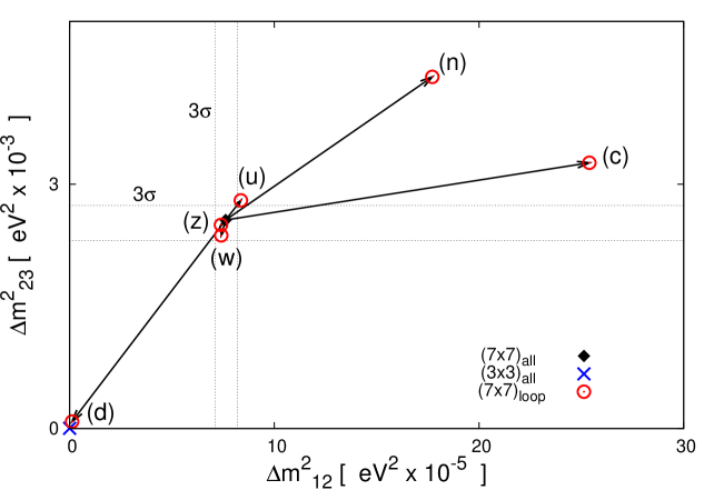
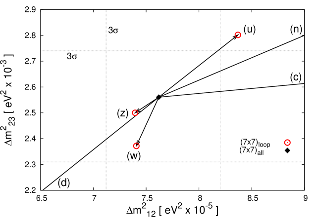
Figure 1: Influence of loop corrections on Δmatm2Δsubscriptsuperscript𝑚2𝑎𝑡𝑚\Delta m^{2}_{atm} and Δmsol2Δsubscriptsuperscript𝑚2𝑠𝑜𝑙\Delta m^{2}_{sol} in the whole 7×7777\times 7 mass matrix. The lower figure is a zoom-in of the top one.

In Fig. 1 one works in the plane formed by the atmospheric Δm232Δsubscriptsuperscript𝑚223\Delta m^{2}_{23} and the solar Δm122Δsubscriptsuperscript𝑚212\Delta m^{2}_{12} neutrino mass parameters. In vertical and horizontal dashed lines the 3σ3𝜎3\sigma experimental limits for these parameters are shown. At approximately the center of this allowed region one has the predictions from our scenario using the full 7×7777\times 7 mass matrix, represented by a dark (black) diamond. Flowing from this point one has several arrows ending in circles (red), one for each loop. What it is done here is to omit in every entry of the 7×7777\times 7 mass matrix the contribution from the corresponding loop, and show the prediction for the mass differences in these conditions.

The contributions from the bottom-sbottom, neutralino-neutral scalar, and chargino-charged scalar loops are large as expected (Fig. 1-top). The not-so-known effect is the importance of the top-stop loops, which are large enough to move the prediction outside the 3-σ𝜎\sigma region when it is not included (Fig. 1-bottom). The reason for the unexpectedness of this result is that these loops do not contribute to the neutrino masses in the 3×3333\times 3 approach, which is very popular. The contribution by these loops appears through the last term in eq. (2.24), which is of third order. As explain in the next section, this contribution is proportional to the top quark Yukawa coupling and needs the presence of the bottom-sbottom loops as well. One may also see that in this particular scenario, the 3×3333\times 3 approximation does not work since it gives a prediction for the solar and atmospheric mass squared parameters which are off by several orders of magnitude, represented by a cross (blue).
Refer to caption
Figure 2: Influence of loop corrections on Δmatm2Δsubscriptsuperscript𝑚2𝑎𝑡𝑚\Delta m^{2}_{atm} and Δmsol2Δsubscriptsuperscript𝑚2𝑠𝑜𝑙\Delta m^{2}_{sol} in a given matrix element of the 7×7777\times 7 mass matrix.

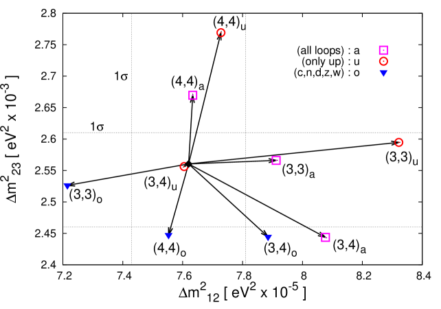
Second of all, in Fig. 2 a similar process is performed. This time a specific loop in a given entry in the 7×7777\times 7 mass matrix is omitted. For the arrows ending in a square (magenta), one is omitting all the loops at each (3,3)33(3,3), (3,4)34(3,4) and (4,4)44(4,4) matrix elements. For the arrows ending in a circle (red), one is omitting the up-sup loops for the same matrix elements. Finally, for the arrows ending in a triangle (blue), one is omitting all the loops except up-sup, also for the same matrix elements. The lesson draw from the figure is that the importance of the top-stop loops lies in the higgsino section of the mass matrix. This is clear since the corrections in that sector are proportional to the top quark Yukawa coupling.

When it is convenient to work with a 3×3333\times 3 neutrino mass matrix, the second and third order terms in eq. (2.24) should be included, because they are numerically important. Once that is done, the precision obtained with the 7×7777\times 7 approach is recovered.

Observable 7×7777\times 7 3×3333\times 3 3×3full3subscript3𝑓𝑢𝑙𝑙{3\times 3}_{full}
Δmatm2Δsubscriptsuperscript𝑚2𝑎𝑡𝑚\Delta m^{2}_{atm} 2.56×1032.56superscript1032.56\times 10^{-3} 2.02×1062.02superscript1062.02\times 10^{-6} 2.56×1032.56superscript1032.56\times 10^{-3}
Δmsol2Δsubscriptsuperscript𝑚2𝑠𝑜𝑙\Delta m^{2}_{sol} 7.62×1057.62superscript1057.62\times 10^{-5} 1.53×1081.53superscript1081.53\times 10^{-8} 7.57×1057.57superscript1057.57\times 10^{-5}
sin2θatmsuperscript2subscript𝜃𝑎𝑡𝑚\sin^{2}\theta_{atm} 0.6390.6390.639 0.8390.8390.839 0.6400.6400.640
sin2θsolsuperscript2subscript𝜃𝑠𝑜𝑙\sin^{2}\theta_{sol} 0.3050.3050.305 0.4420.4420.442 0.3030.3030.303
sin2θreasuperscript2subscript𝜃𝑟𝑒𝑎\sin^{2}\theta_{rea} 0.0240.0240.024 0.4070.4070.407 0.0240.0240.024
Table 5: Neutrino observables calculated in the different approaches.

In Table 5 the prediction for the neutrino observables in the same scenario introduced before is shown. In the second and third column the usual 7×7777\times 7 and 3×3333\times 3 approaches are shown. In the last column the extra terms in eq. (2.24), calling the approach as 3×3full3subscript3𝑓𝑢𝑙𝑙3\times 3_{full}, is included. It is clear the recovery in precision.

The second order is given by the third term in eq. (2.24). In the chosen scenario, this term is also very important. That can be understood from Fig. 1-top and Fig. 2. In Fig. 1-top the effect of the first order is seen by the cross (blue). The fact that this prediction is so small is an indication that this first order effect is also small. On the other hand, the effect of the third order seen in Fig. 2, although large when compared to experimental errors, is small compared to full expansion (first plus second plus third order), therefore, the second order is very important.

4 Algebraic Approximations

Here, approximated algebraic expressions for second and third order terms from the top-stop contribution to the solar mass are found, in order to better understand the numeric results shown in the previous section. These numerical calculations show that top-stop loops contribute importantly.

The contribution from top-stop loops to the second order term in eq. (2.24) is studied. In the higgsino sector the relevant matrix elements of the inverse neutralino mass matrix, following the Appendix B is,

(Mχ0)341=(Mχ0)4311μ.subscriptsuperscriptsuperscriptsubscriptM𝜒0134subscriptsuperscriptsuperscriptsubscriptM𝜒01431𝜇({\mathrm{M}}_{\chi}^{0})^{-1}_{34}=({\mathrm{M}}_{\chi}^{0})^{-1}_{43}\approx-\frac{1}{\mu}. (4.26)

Therefore,

[δmMχ01δmT]ijsubscriptdelimited-[]𝛿𝑚superscriptsubscriptMsuperscript𝜒01𝛿superscript𝑚𝑇𝑖𝑗\displaystyle-\left[\delta m\,{\mathrm{M}}_{\chi^{0}}^{-1}\,\delta m^{T}\right]_{ij} =\displaystyle= 1μ[δmi3δmj4+δmi4δmj3]ij=1μ(δm3,Λtt~)(δm4,Λtt~)ΛiΛj,1𝜇subscriptdelimited-[]𝛿subscript𝑚𝑖3𝛿subscript𝑚𝑗4𝛿subscript𝑚𝑖4𝛿subscript𝑚𝑗3𝑖𝑗1𝜇𝛿superscriptsubscript𝑚3Λ𝑡~𝑡𝛿superscriptsubscript𝑚4Λ𝑡~𝑡subscriptΛ𝑖subscriptΛ𝑗\displaystyle\frac{1}{\mu}\Big{[}\delta m_{i3}\delta m_{j4}+\delta m_{i4}\delta m_{j3}\Big{]}_{ij}=\frac{1}{\mu}(\delta m_{3,\Lambda}^{t\tilde{t}})(\delta m_{4,\Lambda}^{t\tilde{t}})\,\Lambda_{i}\Lambda_{j}\,, (4.27)

and it does not contribute to the solar mass, since it is proportional to ΛiΛjsubscriptΛ𝑖subscriptΛ𝑗\Lambda_{i}\Lambda_{j}. In fact, since the top-stop coupling to neutrinos does not include ϵitalic-ϵ\epsilon terms, none of the quantities δmijtt~𝛿superscriptsubscript𝑚𝑖𝑗𝑡~𝑡\delta m_{ij}^{t\tilde{t}} will produce a contribution to the solar mass. Thus, third order term is studied next.

The third order term in eq. (2.24), given by

δm(Mχd,0)1δMχ(Mχd,0)1δmT,𝛿𝑚superscriptsubscriptsuperscriptM𝑑0𝜒1𝛿subscript𝑀𝜒superscriptsubscriptsuperscriptM𝑑0𝜒1𝛿superscript𝑚𝑇\delta m\,({\mathrm{M}}^{d,0}_{\chi})^{-1}\,\delta M_{\chi}\,({\mathrm{M}}^{d,0}_{\chi})^{-1}\delta m^{T}\,, (4.28)

is written in the basis where the tree-level neutralino mass matrix has already been diagonalized. If work is to be done in the original basis instead, the term to analyze is,

δm(Mχ0)1δMχ(Mχ0)1δmT,𝛿𝑚superscriptsubscriptsuperscriptM0𝜒1𝛿subscript𝑀𝜒superscriptsubscriptsuperscriptM0𝜒1𝛿superscript𝑚𝑇\delta m\,({\mathrm{M}}^{0}_{\chi})^{-1}\,\delta M_{\chi}\,({\mathrm{M}}^{0}_{\chi})^{-1}\delta m^{T}\,, (4.29)

where δm𝛿𝑚\delta m (and δMχ~𝛿subscript𝑀~𝜒\delta M_{\tilde{\chi}}) in eq. (4.28) is written in the diagonal basis, while δm𝛿𝑚\delta m (and δMχ~𝛿subscript𝑀~𝜒\delta M_{\tilde{\chi}}) in eq. (4.29) is written in the original basis. The same notation is used for both out of simplicity.

In order to algebraically understand the issues mentioned in the previous section a few approximations are performed. First, notice that down-type quarks contribute to δm𝛿𝑚\delta m with a term proportional to ϵisubscriptitalic-ϵ𝑖\epsilon_{i}, while up-type quarks do not, as can be seen from the Appendix A. Thus, in this approximation,

(δm)ij=δmi3δj3.subscript𝛿𝑚𝑖𝑗𝛿subscript𝑚𝑖3subscript𝛿𝑗3(\delta m)_{ij}=\delta m_{i3}\,\delta_{j3}. (4.30)

Second, notice that the (4,4)44(4,4) matrix element in the neutralino sector makes a strong numerical effect on the neutrino parameters, and up-type quarks contribute to it. To isolate this effect it is assumed,

(δMχ)ij=δMχ,44δi4δj4.subscript𝛿subscript𝑀𝜒𝑖𝑗𝛿subscript𝑀𝜒44subscript𝛿𝑖4subscript𝛿𝑗4(\delta M_{\chi})_{ij}=\delta M_{\chi,44}\,\delta_{i4}\,\delta_{j4}. (4.31)

With this, the contribution from top-stop loops to the third order term in eq. (2.24) is,

[δm(Mχ0)1δMχ(Mχ0)1δmT]ijsubscriptdelimited-[]𝛿𝑚superscriptsubscriptsuperscriptM0𝜒1𝛿subscript𝑀𝜒superscriptsubscriptsuperscriptM0𝜒1𝛿superscript𝑚𝑇𝑖𝑗\displaystyle\left[\delta m\,({\mathrm{M}}^{0}_{\chi})^{-1}\,\delta M_{\chi}\,({\mathrm{M}}^{0}_{\chi})^{-1}\,\delta m^{T}\right]_{ij} \displaystyle\approx δMχ,44tt~(Mχ0)342(δmi3bb~)(δmj3bb~)𝛿superscriptsubscript𝑀𝜒44𝑡~𝑡subscriptsuperscriptsubscriptsuperscriptM0𝜒234𝛿superscriptsubscript𝑚𝑖3𝑏~𝑏𝛿superscriptsubscript𝑚𝑗3𝑏~𝑏\displaystyle\delta M_{\chi,44}^{t\tilde{t}}\,({\mathrm{M}}^{0}_{\chi})^{-2}_{34}(\delta m_{i3}^{b\tilde{b}})\,(\delta m_{j3}^{b\tilde{b}})
\displaystyle\approx δMχ,44tt~(Mχ0)342[δm3,Λbb~Λi+δm3,ϵbb~ϵi][δm3,Λbb~Λj+δm3,ϵbb~ϵj].𝛿superscriptsubscript𝑀𝜒44𝑡~𝑡subscriptsuperscriptsubscriptsuperscriptM0𝜒234delimited-[]𝛿superscriptsubscript𝑚3Λ𝑏~𝑏subscriptΛ𝑖𝛿superscriptsubscript𝑚3italic-ϵ𝑏~𝑏subscriptitalic-ϵ𝑖delimited-[]𝛿superscriptsubscript𝑚3Λ𝑏~𝑏subscriptΛ𝑗𝛿superscriptsubscript𝑚3italic-ϵ𝑏~𝑏subscriptitalic-ϵ𝑗\displaystyle\delta M_{\chi,44}^{t\tilde{t}}\,({\mathrm{M}}^{0}_{\chi})^{-2}_{34}\Big{[}\delta m_{3,\Lambda}^{b\tilde{b}}\Lambda_{i}+\delta m_{3,\epsilon}^{b\tilde{b}}\epsilon_{i}\Big{]}\Big{[}\delta m_{3,\Lambda}^{b\tilde{b}}\Lambda_{j}+\delta m_{3,\epsilon}^{b\tilde{b}}\epsilon_{j}\Big{]}.

Approximating further the ϵϵitalic-ϵitalic-ϵ\epsilon\epsilon term is,

[δm(Mχ0)1δMχ(Mχ0)1δmT]ijϵϵsuperscriptsubscriptdelimited-[]𝛿𝑚superscriptsubscriptsuperscriptM0𝜒1𝛿subscript𝑀𝜒superscriptsubscriptsuperscriptM0𝜒1𝛿superscript𝑚𝑇𝑖𝑗italic-ϵitalic-ϵ\displaystyle\left[\delta m\,({\mathrm{M}}^{0}_{\chi})^{-1}\,\delta M_{\chi}\,({\mathrm{M}}^{0}_{\chi})^{-1}\,\delta m^{T}\right]_{ij}^{\epsilon\epsilon} \displaystyle\approx [ncht232π2×2×2μ][1μ]2[nchb264π2μ×2×2μ]2ϵiϵjdelimited-[]subscript𝑛𝑐superscriptsubscript𝑡232superscript𝜋222𝜇superscriptdelimited-[]1𝜇2superscriptdelimited-[]subscript𝑛𝑐superscriptsubscript𝑏264superscript𝜋2𝜇22𝜇2subscriptitalic-ϵ𝑖subscriptitalic-ϵ𝑗\displaystyle\left[\frac{n_{c}h_{t}^{2}}{32\pi^{2}}\times 2\times 2\mu\right]\,\left[-\frac{1}{\mu}\right]^{2}\,\left[\frac{n_{c}h_{b}^{2}}{64\pi^{2}\mu}\times 2\times 2\mu\right]^{2}\epsilon_{i}\epsilon_{j} (4.33)
=\displaystyle= 2nc3ht2hb4(16π2)3μϵiϵjnc3g6mt2mb44(16π2)3sβ2cβ4mW6μϵiϵj2superscriptsubscript𝑛𝑐3superscriptsubscript𝑡2superscriptsubscript𝑏4superscript16superscript𝜋23𝜇subscriptitalic-ϵ𝑖subscriptitalic-ϵ𝑗superscriptsubscript𝑛𝑐3superscript𝑔6superscriptsubscript𝑚𝑡2superscriptsubscript𝑚𝑏44superscript16superscript𝜋23superscriptsubscript𝑠𝛽2superscriptsubscript𝑐𝛽4superscriptsubscript𝑚𝑊6𝜇subscriptitalic-ϵ𝑖subscriptitalic-ϵ𝑗\displaystyle\frac{2n_{c}^{3}h_{t}^{2}h_{b}^{4}}{(16\pi^{2})^{3}\mu}\epsilon_{i}\epsilon_{j}\approx\frac{n_{c}^{3}g^{6}m_{t}^{2}m_{b}^{4}}{4(16\pi^{2})^{3}s_{\beta}^{2}c_{\beta}^{4}m_{W}^{6}\mu}\epsilon_{i}\epsilon_{j}
\displaystyle\approx 102tβ4ϵiϵjμeV,superscript102superscriptsubscript𝑡𝛽4subscriptitalic-ϵ𝑖subscriptitalic-ϵ𝑗𝜇eV\displaystyle 10^{-2}\frac{t_{\beta}^{4}\epsilon_{i}\epsilon_{j}}{\mu}\,\,{\text{eV}}\,,

which gives the same order of magnitude of the solar mass squared difference, thus it should not be neglected.

5 General Scan over Parameter Space

In order to see the 0 of the different approximations a general scan over the parameter space was made. As it was explained in section 3 the code SUSPECT [28] was used for the running of the RpC supersymmetric parameters, and our own code for the neutrino observables from the R-Parity violating parameters (since R-Parity violation is small, the use of MSSM RGEs for the RpC parameters is a good approximation). Randomly selected values for the RpC parameters at the GUT scale are generated and SUSPECT is used to find their counterpart at the weak scale, including a correct electroweak symmetry breaking. At this point the following cuts are added: the Higgs mass, 124<mh<126124subscript𝑚126124<m_{h}<126 GeV, ΔρΔ𝜌\Delta\rho, ΔaμΔsubscript𝑎𝜇\Delta a_{\mu}, B(bsγ)𝐵𝑏𝑠𝛾B(b\rightarrow s\gamma) (see first paragraph in section 3). Then, randomly generated values for the RpV parameters are added to the 0 parameters, and with all of them a seed point in parameter space at the weak scale is defined. Using an implementation of the Markov chain [34] and starting from the seed point just described, a movement in steps is implemented, minimizing a χ2superscript𝜒2\chi^{2} function that includes neutrino experimental parameters only (mass squared differences and mixing angles) towards a final point that satisfy neutrino physics. Finally, cuts on the masses of the following supersymmetric particles are implemented mχ1+>600subscript𝑚subscriptsuperscript𝜒1600m_{\chi^{+}_{1}}>600 GeV, mχ10>300subscript𝑚subscriptsuperscript𝜒01300m_{\chi^{0}_{1}}>300 GeV, m~>1subscript𝑚~1m_{\tilde{\ell}}>1 TeV, mq~>2subscript𝑚~𝑞2m_{\tilde{q}}>2 TeV, mg~>2subscript𝑚~𝑔2m_{\tilde{g}}>2 TeV [35, 36]

Following section 3, some of the parameters at the weak scale that define the points that satisfy all cuts lie in intervals described in Table 6.

Parameter Minimum Maximum Units
tanβ𝛽\tan\beta 9.119.119.11 48.848.848.8 -
μ𝜇\mu 655655655 449544954495 GeV
M1subscript𝑀1M_{1} 313313313 897897897 GeV
M2subscript𝑀2M_{2} 567567567 159715971597 GeV
M3subscript𝑀3M_{3} 329632963296 595259525952 GeV
MQsubscript𝑀𝑄M_{Q} 286228622862 609360936093 GeV
MUsubscript𝑀𝑈M_{U} 161616161616 583458345834 GeV
MDsubscript𝑀𝐷M_{D} 242724272427 645864586458 GeV
MLsubscript𝑀𝐿M_{L} 100710071007 517651765176 GeV
MRsubscript𝑀𝑅M_{R} 102410241024 489948994899 GeV
ϵ1subscriptitalic-ϵ1\epsilon_{1} 0.1170.117-0.117 0.1580.1580.158 GeV
ϵ2subscriptitalic-ϵ2\epsilon_{2} 0.2350.235-0.235 0.3030.3030.303 GeV
ϵ3subscriptitalic-ϵ3\epsilon_{3} 0.1560.156-0.156 0.2770.2770.277 GeV
Λ1subscriptΛ1\Lambda_{1} 0.1020.102-0.102 0.1120.1120.112 GeV2
Λ2subscriptΛ2\Lambda_{2} 0.1180.118-0.118 0.1240.1240.124 GeV2
Λ3subscriptΛ3\Lambda_{3} 0.1300.130-0.130 0.1160.1160.116 GeV2
Table 6: Intervals for each parameters at the low scale.

Similarly, the interval for some of the physical masses are indicated in Table 7.

Particle Minimum Maximum
hh 124124124 126126126
A𝐴A 109710971097 412841284128
χ10subscriptsuperscript𝜒01\chi^{0}_{1} 310310310 897897897
χ1+subscriptsuperscript𝜒1\chi^{+}_{1} 601601601 165116511651
ν~τsubscript~𝜈𝜏\tilde{\nu}_{\tau} 100510051005 517651765176
τ~1subscript~𝜏1\tilde{\tau}_{1} 100110011001 480048004800
t~1subscript~𝑡1\tilde{t}_{1} 297329732973 623462346234
b~1subscript~𝑏1\tilde{b}_{1} 321632163216 655965596559
Table 7: Part of the supersymmetric spectrum (in GeV).

The high value for the squark masses (and soft mass parameters as well) is due to the Higgs mass, which needs high squarks masses in order to reach the value mh125similar-tosubscript𝑚125m_{h}\sim 125 GeV. For the same reason (although contributing at two loops), the gluino mass is also high: mg~>3500subscript𝑚~𝑔3500m_{\tilde{g}}>3500 GeV including radiative corrections.

Refer to caption
Figure 3: Solar mass squared difference calculated with the 3×3333\times 3 approximation, in comparison with the one calculated with the 7×7777\times 7 matrix.

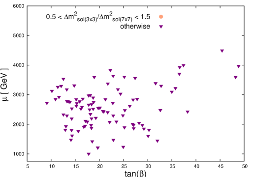
In Fig. 3 the 0 of the 3×3333\times 3 approximation in the μ𝜇\mu-tanβ𝛽\tan\beta plane is shown. Different colors according to the ratio Δmsol(3×3)2/Δmsol(7×7)2Δsubscriptsuperscript𝑚2𝑠𝑜𝑙33Δsubscriptsuperscript𝑚2𝑠𝑜𝑙77\Delta m^{2}_{sol(3\times 3)}/\Delta m^{2}_{sol(7\times 7)} are displayed (in principle), i.e., the solar mass squared difference calculated with the 3×3333\times 3 approximation in comparison with the same neutrino observable calculated with the full 7×7777\times 7 matrix. It is seen that the solar mass calculated with the 3×3333\times 3 approximation is always off by more than 50%percent5050\%. In fact, it is observed in the scan that it is always smaller, and very often the error is much larger than 50%percent5050\%. Considering the experimental errors in the measurement of the solar mass, the 3×3333\times 3 approximation is not reliable anymore.
Refer to caption
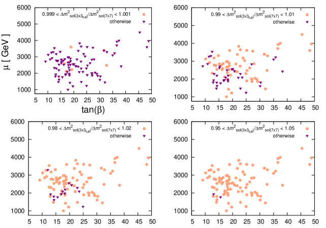
Figure 4: Solar mass squared difference calculated with the 3×3full3subscript3𝑓𝑢𝑙𝑙3\times 3_{full} approximation, in comparison with the one calculated with the 7×7777\times 7 matrix.

In Fig. 4 a similar comparison is made, but this time for the solar mass calculated with the 3×3full3subscript3𝑓𝑢𝑙𝑙3\times 3_{full} approximation. Furthermore, displayed are four quadrants that refer to four different values for the error: 0.1%percent0.10.1\%, 1%percent11\%, 2%percent22\%, and 5%percent55\%. In the lower-right frame (5%percent55\%) it is seen that the 3×3full3subscript3𝑓𝑢𝑙𝑙3\times 3_{full} approximation is much better than the usual 3×3333\times 3: almost all the time the solar mass lies within 5%percent55\% with respect to the calculated with the 7×7777\times 7 matrix. At the level of 0.1%percent0.10.1\% (upper-left), even the 3×3full3subscript3𝑓𝑢𝑙𝑙3\times 3_{full} approximation fails in comparison with 7×7777\times 7. In addition, from the sequence of frames in Fig. 4 it can be concluded that the 3×3full3subscript3𝑓𝑢𝑙𝑙3\times 3_{full} is more reliable at high values of tanβ𝛽\tan\beta. This can be understood from the fact that at high values of tanβ𝛽\tan\beta the bottom quark Yukawa coupling is larger and, therefore, bottom quark effects are more 0. This makes the 3×3full3subscript3𝑓𝑢𝑙𝑙3\times 3_{full} approximation more reliable, and simultaneously the 3×3333\times 3 approximation less reliable, at high values of tanβ𝛽\tan\beta.

Refer to caption
Figure 5: Effect of the removal of the up-type quark and squark loops.

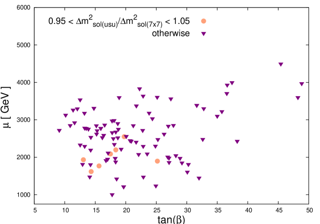
Finally in Fig. 5 it is seen the effect of the up type quarks and squarks on the solar mass, displayed in the same μtanβ𝜇𝛽\mu-\tan\beta plane. Notice that these loops contribute to the solar mass only via the third order term. In the scan the effect of removing all together the up-sup loops from the 7×7777\times 7 matrix is shown, and a 0 with the solar mass calculated with the full 7×7777\times 7 matrix is done. In most of the points the effect of the up-sup loops is large (larger than 5%percent55\% in the figure).

6 Conclusions

It was shown that the 3×3333\times 3 approach in the calculation of neutrino masses in the MSSM with BRpV, in the light of the present accuracy of the experimental results, sometimes does not give an acceptable answer. This was understood by studying the 3×3333\times 3 second and third order terms in the block diagonalization of the 7×7777\times 7 mass matrix. When it is convenient to work with 3×3333\times 3 matrices, it was shown also that keeping these terms gives a very similar result compared to the ones extracted from the 7×7777\times 7 neutrino mass matrix. In addition, in the 3×3333\times 3 approach, the top-stop loops do not contribute, nevertheless, they can be numerically important. These loops contribute through the already mentioned third order term, and it was shown that the contribution is dependent on the bottom as well as the top quark Yukawa couplings. The second order term in eq. (2.24) can also be very important. In fact, a scenario was chosen where it is crucial. All these issues motivate a two-loop calculation of neutrino masses in this model. A scan over parameter space is made to show that the conclusions are general, and not driven by the chosen point shown in section 3. Most of these numerical effect come from the high value of the Higgs boson mass.

Acknowledgments

This work was supported by Fondecyt grants No. 11110472, 1100837 and 1141190, Anillo “AtlasAndino” ACT1102, UTFSM-DGIP grant No. 11.12.39, and Conicyt Doctorate Grant.

Appendix A Squark Loop Contributions

A.1 Top-stop loops in δMχ𝛿subscript𝑀𝜒\delta M_{\chi}

It is numerically observed that among the 16 matrix elements of δMχ𝛿subscript𝑀𝜒\delta M_{\chi}, the (4,4)44(4,4) is the one that gives the largest contribution. In addition, the top-stop loops have an important effect on this matrix element. In order to algebraically understand the phenomena, this contribution is calculated. The coupling between neutral fermions and top-stop quarks is,

t~ksubscript~𝑡𝑘\tilde{t}_{k}t𝑡tFj0subscriptsuperscript𝐹0𝑗F^{0}_{j}

=i[OLjktnt~(1γ5)2+ORjktnt~(1+γ5)2],absent𝑖delimited-[]subscriptsuperscript𝑂𝑡𝑛~𝑡𝐿𝑗𝑘1subscript𝛾52subscriptsuperscript𝑂𝑡𝑛~𝑡𝑅𝑗𝑘1subscript𝛾52=\,i\,\Big{[}O^{tn\tilde{t}}_{Ljk}\frac{(1-\gamma_{5})}{2}+O^{tn\tilde{t}}_{Rjk}\frac{(1+\gamma_{5})}{2}\Big{]},

with

OLjktnt~subscriptsuperscript𝑂𝑡𝑛~𝑡𝐿𝑗𝑘\displaystyle O^{tn\tilde{t}}_{Ljk} =\displaystyle= ηj4gtW32𝒩j1Rk2t~ηjht𝒩j4Rk1t~,subscript𝜂𝑗4𝑔subscript𝑡𝑊32subscriptsuperscript𝒩𝑗1subscriptsuperscript𝑅~𝑡𝑘2subscript𝜂𝑗subscript𝑡subscriptsuperscript𝒩𝑗4subscriptsuperscript𝑅~𝑡𝑘1\displaystyle\eta_{j}\frac{4gt_{W}}{3\sqrt{2}}{\cal N}^{*}_{j1}R^{\tilde{t}}_{k2}-\eta_{j}h_{t}{\cal N}^{*}_{j4}R^{\tilde{t}}_{k1}\,,
ORjktnt~subscriptsuperscript𝑂𝑡𝑛~𝑡𝑅𝑗𝑘\displaystyle O^{tn\tilde{t}}_{Rjk} =\displaystyle= g2(𝒩j2+13tW𝒩j1)Rk1t~ht𝒩j4Rk2t~,𝑔2subscript𝒩𝑗213subscript𝑡𝑊subscript𝒩𝑗1subscriptsuperscript𝑅~𝑡𝑘1subscript𝑡subscript𝒩𝑗4subscriptsuperscript𝑅~𝑡𝑘2\displaystyle-\frac{g}{\sqrt{2}}\left({\cal N}_{j2}+\frac{1}{3}t_{W}{\cal N}_{j1}\right)R^{\tilde{t}}_{k1}-h_{t}{\cal N}_{j4}R^{\tilde{t}}_{k2}\,, (1.34)

and where htsubscript𝑡h_{t} is the top quark Yukawa coupling, Rt~superscript𝑅~𝑡R^{\tilde{t}} is the (assumed real) 2×2222\times 2 rotation matrix that diagonalizes the stop quark mass matrix, 𝒩𝒩{\cal N} is the (assumed real) 7×7777\times 7 rotation matrix that diagonalizes the neutralino sector, and ηjsubscript𝜂𝑗\eta_{j} is the sign of the corresponding fermion j𝑗j. Notice that the complex conjugated 𝒩superscript𝒩{\cal N}^{*} is kept only for reference, since one assumes it is real. If this coupling is specialized to the case when the neutral fermion is a neutralino one finds,

t~ksubscript~𝑡𝑘\tilde{t}_{k}t𝑡tχj0subscriptsuperscript𝜒0𝑗\chi^{0}_{j}

=i[OLjktχt~(1γ5)2+ORjktχt~(1+γ5)2],absent𝑖delimited-[]subscriptsuperscript𝑂𝑡𝜒~𝑡𝐿𝑗𝑘1subscript𝛾52subscriptsuperscript𝑂𝑡𝜒~𝑡𝑅𝑗𝑘1subscript𝛾52=\,i\,\Big{[}O^{t\chi\tilde{t}}_{Ljk}\frac{(1-\gamma_{5})}{2}+O^{t\chi\tilde{t}}_{Rjk}\frac{(1+\gamma_{5})}{2}\Big{]},

with

OLjktχt~subscriptsuperscript𝑂𝑡𝜒~𝑡𝐿𝑗𝑘\displaystyle O^{t\chi\tilde{t}}_{Ljk} =\displaystyle= ηj4gtW32Nj1Rk2t~ηjhtNj4Rk1t~,subscript𝜂𝑗4𝑔subscript𝑡𝑊32subscriptsuperscript𝑁𝑗1subscriptsuperscript𝑅~𝑡𝑘2subscript𝜂𝑗subscript𝑡subscriptsuperscript𝑁𝑗4subscriptsuperscript𝑅~𝑡𝑘1\displaystyle\eta_{j}\frac{4gt_{W}}{3\sqrt{2}}N^{*}_{j1}R^{\tilde{t}}_{k2}-\eta_{j}h_{t}N^{*}_{j4}R^{\tilde{t}}_{k1}\,,
ORjktχt~subscriptsuperscript𝑂𝑡𝜒~𝑡𝑅𝑗𝑘\displaystyle O^{t\chi\tilde{t}}_{Rjk} =\displaystyle= g2(Nj2+13tWNj1)Rk1t~htNj4Rk2t~.𝑔2subscript𝑁𝑗213subscript𝑡𝑊subscript𝑁𝑗1subscriptsuperscript𝑅~𝑡𝑘1subscript𝑡subscript𝑁𝑗4subscriptsuperscript𝑅~𝑡𝑘2\displaystyle-\frac{g}{\sqrt{2}}\left(N_{j2}+\frac{1}{3}t_{W}N_{j1}\right)R^{\tilde{t}}_{k1}-h_{t}N_{j4}R^{\tilde{t}}_{k2}\,. (1.35)

In this case, N𝑁N is the (real) 4×4444\times 4 rotation matrix that diagonalizes the neutralino mass sub-matrix, and ηjsubscript𝜂𝑗\eta_{j} is the sign of the j𝑗j-th neutralino mass. The relevant loop is formed with those couplings,

t~ksubscript~𝑡𝑘\tilde{t}_{k}t𝑡tχi0subscriptsuperscript𝜒0𝑖\chi^{0}_{i}χj0subscriptsuperscript𝜒0𝑗\chi^{0}_{j}

=iΣijtt~(p2),absent𝑖superscriptsubscriptΣ𝑖𝑗𝑡~𝑡superscript𝑝2=\,i\,\Sigma_{ij}^{t\tilde{t}}(p^{2}),

with,

Σijtt~(p2)=ncht2Ni4Nj416π2k=12[mtRk1t~Rk2t~(ηiPL+ηjPR)B0ptt~(Rk1t~2ηiηjPL+Rk2t~2PR)B1ptt~]+superscriptsubscriptΣ𝑖𝑗𝑡~𝑡superscript𝑝2subscript𝑛𝑐superscriptsubscript𝑡2subscript𝑁𝑖4subscript𝑁𝑗416superscript𝜋2superscriptsubscript𝑘12delimited-[]subscript𝑚𝑡subscriptsuperscript𝑅~𝑡𝑘1subscriptsuperscript𝑅~𝑡𝑘2subscript𝜂𝑖subscript𝑃𝐿subscript𝜂𝑗subscript𝑃𝑅superscriptsubscript𝐵0𝑝𝑡~𝑡italic-p̸subscriptsuperscript𝑅~𝑡2𝑘1subscript𝜂𝑖subscript𝜂𝑗subscript𝑃𝐿subscriptsuperscript𝑅~𝑡2𝑘2subscript𝑃𝑅superscriptsubscript𝐵1𝑝𝑡~𝑡\Sigma_{ij}^{t\tilde{t}}(p^{2})=\frac{n_{c}h_{t}^{2}N_{i4}N_{j4}}{16\pi^{2}}\sum_{k=1}^{2}\left[m_{t}R^{\tilde{t}}_{k1}R^{\tilde{t}}_{k2}(\eta_{i}P_{L}+\eta_{j}P_{R})B_{0}^{pt\tilde{t}}-\not{p}(R^{\tilde{t}2}_{k1}\eta_{i}\eta_{j}P_{L}+R^{\tilde{t}2}_{k2}P_{R})B_{1}^{pt\tilde{t}}\right]+... (1.36)

Here the three dots mean that only the terms proportional to ht2superscriptsubscript𝑡2h_{t}^{2} are shown. Also, the fact that the matrix N𝑁N is real was already used.

When evaluating δMχij𝛿superscriptsubscript𝑀𝜒𝑖𝑗\delta M_{\chi}^{ij} it should be understood that in the basis where the neutralinos are diagonal, one wants to evaluate the neutralino mass at p2superscript𝑝2p^{2}, and symmetrize over i𝑖i and j𝑗j. Thus,

δMχij𝛿superscriptsubscript𝑀𝜒𝑖𝑗\displaystyle\delta M_{\chi}^{ij} =\displaystyle= ncht2Ni4Nj432π2k=12{12mtRk1t~Rk2t~(ηi+ηj)(B0χitt~+B0χjtt~)\displaystyle\frac{n_{c}h_{t}^{2}N_{i4}N_{j4}}{32\pi^{2}}\sum_{k=1}^{2}\bigg{\{}-\frac{1}{2}m_{t}R^{\tilde{t}}_{k1}R^{\tilde{t}}_{k2}(\eta_{i}+\eta_{j})\left(B_{0}^{\chi_{i}t\tilde{t}}+B_{0}^{\chi_{j}t\tilde{t}}\right) (1.37)
+12(Rk1t~2ηiηj+Rk2t~2)(mχi0B1χitt~+mχj0B1χjtt~)},\displaystyle\qquad\qquad\qquad\qquad+\frac{1}{2}(R^{\tilde{t}2}_{k1}\eta_{i}\eta_{j}+R^{\tilde{t}2}_{k2})\left(m_{\chi^{0}_{i}}B_{1}^{\chi_{i}t\tilde{t}}+m_{\chi^{0}_{j}}B_{1}^{\chi_{j}t\tilde{t}}\right)\bigg{\}}\,,
=\displaystyle= ncht2Ni4Nj432π2k=12{12mtst~ct~(1)k(ηi+ηj)(B0χitt~+B0χjtt~)\displaystyle\frac{n_{c}h_{t}^{2}N_{i4}N_{j4}}{32\pi^{2}}\sum_{k=1}^{2}\bigg{\{}\frac{1}{2}m_{t}s_{\tilde{t}}c_{\tilde{t}}(-1)^{k}(\eta_{i}+\eta_{j})\left(B_{0}^{\chi_{i}t\tilde{t}}+B_{0}^{\chi_{j}t\tilde{t}}\right)
+12(ct~2ηiηj+st~2)(mχi0B1χitt~+mχj0B1χjtt~)}.\displaystyle\qquad\qquad\qquad\qquad+\frac{1}{2}(c_{\tilde{t}}^{2}\eta_{i}\eta_{j}+s_{\tilde{t}}^{2})\left(m_{\chi^{0}_{i}}B_{1}^{\chi_{i}t\tilde{t}}+m_{\chi^{0}_{j}}B_{1}^{\chi_{j}t\tilde{t}}\right)\bigg{\}}\,.

The contribution to the (4,4)44(4,4) neutrino/neutralino mass matrix element is therefore,

δMχ44=ncht2N44232π2k=12{2mtst~ct~(1)kη4B0(mχ402;mt2,mt~k2)+mχ40B1(mχ402;mt2,mt~k2)},𝛿superscriptsubscript𝑀𝜒44subscript𝑛𝑐superscriptsubscript𝑡2superscriptsubscript𝑁44232superscript𝜋2superscriptsubscript𝑘122subscript𝑚𝑡subscript𝑠~𝑡subscript𝑐~𝑡superscript1𝑘subscript𝜂4subscript𝐵0superscriptsubscript𝑚subscriptsuperscript𝜒042superscriptsubscript𝑚𝑡2superscriptsubscript𝑚subscript~𝑡𝑘2subscript𝑚subscriptsuperscript𝜒04subscript𝐵1superscriptsubscript𝑚subscriptsuperscript𝜒042superscriptsubscript𝑚𝑡2superscriptsubscript𝑚subscript~𝑡𝑘2\delta M_{\chi}^{44}=\frac{n_{c}h_{t}^{2}N_{44}^{2}}{32\pi^{2}}\sum_{k=1}^{2}\bigg{\{}2m_{t}s_{\tilde{t}}c_{\tilde{t}}(-1)^{k}\eta_{4}B_{0}(m_{\chi^{0}_{4}}^{2};m_{t}^{2},m_{\tilde{t}_{k}}^{2})+m_{\chi^{0}_{4}}B_{1}(m_{\chi^{0}_{4}}^{2};m_{t}^{2},m_{\tilde{t}_{k}}^{2})\bigg{\}}, (1.38)

which is an approximation for the top-stop loop contribution to δMχ44𝛿superscriptsubscript𝑀𝜒44\delta M_{\chi}^{44}.

A.2 Bottom-sbottom loops in δMχ𝛿subscript𝑀𝜒\delta M_{\chi}

Bottom-sbottom loops contribute importantly to δMχ𝛿subscript𝑀𝜒\delta M_{\chi}, and through it, also contribute importantly to the third term in eq. (2.24). Bottom-sbottom loops contribute importantly to δMν𝛿subscript𝑀𝜈\delta M_{\nu} too, but they are not the focus of this study. The neutral fermion coupling to bottom-sbottom quarks is,

b~ksubscript~𝑏𝑘\tilde{b}_{k}b𝑏bFj0subscriptsuperscript𝐹0𝑗F^{0}_{j}

=i[OLjkbnb~(1γ5)2+ORjkbnb~(1+γ5)2],absent𝑖delimited-[]subscriptsuperscript𝑂𝑏𝑛~𝑏𝐿𝑗𝑘1subscript𝛾52subscriptsuperscript𝑂𝑏𝑛~𝑏𝑅𝑗𝑘1subscript𝛾52=\,i\,\Big{[}O^{bn\tilde{b}}_{Ljk}\frac{(1-\gamma_{5})}{2}+O^{bn\tilde{b}}_{Rjk}\frac{(1+\gamma_{5})}{2}\Big{]},

with

OLjkbnb~subscriptsuperscript𝑂𝑏𝑛~𝑏𝐿𝑗𝑘\displaystyle O^{bn\tilde{b}}_{Ljk} =\displaystyle= ηj2gtW32𝒩j1Rk2b~ηjhb𝒩j3Rk1b~,subscript𝜂𝑗2𝑔subscript𝑡𝑊32superscriptsubscript𝒩𝑗1subscriptsuperscript𝑅~𝑏𝑘2subscript𝜂𝑗subscript𝑏superscriptsubscript𝒩𝑗3subscriptsuperscript𝑅~𝑏𝑘1\displaystyle-\eta_{j}\frac{2gt_{W}}{3\sqrt{2}}{\cal N}_{j1}^{*}R^{\tilde{b}}_{k2}-\eta_{j}h_{b}{\cal N}_{j3}^{*}R^{\tilde{b}}_{k1}\,,
ORjkbnb~subscriptsuperscript𝑂𝑏𝑛~𝑏𝑅𝑗𝑘\displaystyle O^{bn\tilde{b}}_{Rjk} =\displaystyle= g2(𝒩j213tW𝒩j1)Rk1b~hb𝒩j3Rk2b~,𝑔2subscript𝒩𝑗213subscript𝑡𝑊subscript𝒩𝑗1subscriptsuperscript𝑅~𝑏𝑘1subscript𝑏subscript𝒩𝑗3subscriptsuperscript𝑅~𝑏𝑘2\displaystyle\frac{g}{\sqrt{2}}\left({\cal N}_{j2}-\frac{1}{3}t_{W}{\cal N}_{j1}\right)R^{\tilde{b}}_{k1}-h_{b}{\cal N}_{j3}R^{\tilde{b}}_{k2}\,, (1.39)

and where hbsubscript𝑏h_{b} is the bottom quark Yukawa coupling, Rb~superscript𝑅~𝑏R^{\tilde{b}} is the (assumed real) 2×2222\times 2 rotation matrix that diagonalizes the sbottom quark mass matrix, 𝒩𝒩{\cal N} is the already defined (and real) 7×7777\times 7 rotation matrix that diagonalizes the neutralino sector, and ηjsubscript𝜂𝑗\eta_{j} is the already defined sign of the corresponding fermion j𝑗j. Specializing this coupling to the case when the neutral fermion is a neutralino, one finds,

b~ksubscript~𝑏𝑘\tilde{b}_{k}b𝑏bχj0subscriptsuperscript𝜒0𝑗\chi^{0}_{j}

=i[OLjkbχb~(1γ5)2+ORjkbχb~(1+γ5)2],absent𝑖delimited-[]subscriptsuperscript𝑂𝑏𝜒~𝑏𝐿𝑗𝑘1subscript𝛾52subscriptsuperscript𝑂𝑏𝜒~𝑏𝑅𝑗𝑘1subscript𝛾52=\,i\,\Big{[}O^{b\chi\tilde{b}}_{Ljk}\frac{(1-\gamma_{5})}{2}+O^{b\chi\tilde{b}}_{Rjk}\frac{(1+\gamma_{5})}{2}\Big{]},

with

OLjkbχb~subscriptsuperscript𝑂𝑏𝜒~𝑏𝐿𝑗𝑘\displaystyle O^{b\chi\tilde{b}}_{Ljk} =\displaystyle= ηj2gtW32Nj1Rk2b~ηjhbNj3Rk1b~,subscript𝜂𝑗2𝑔subscript𝑡𝑊32superscriptsubscript𝑁𝑗1subscriptsuperscript𝑅~𝑏𝑘2subscript𝜂𝑗subscript𝑏superscriptsubscript𝑁𝑗3subscriptsuperscript𝑅~𝑏𝑘1\displaystyle-\eta_{j}\frac{2gt_{W}}{3\sqrt{2}}N_{j1}^{*}R^{\tilde{b}}_{k2}-\eta_{j}h_{b}N_{j3}^{*}R^{\tilde{b}}_{k1}\,,
ORjkbχb~subscriptsuperscript𝑂𝑏𝜒~𝑏𝑅𝑗𝑘\displaystyle O^{b\chi\tilde{b}}_{Rjk} =\displaystyle= g2(Nj213tWNj1)Rk1b~hbNj3Rk2b~,𝑔2subscript𝑁𝑗213subscript𝑡𝑊subscript𝑁𝑗1subscriptsuperscript𝑅~𝑏𝑘1subscript𝑏subscript𝑁𝑗3subscriptsuperscript𝑅~𝑏𝑘2\displaystyle\frac{g}{\sqrt{2}}\left(N_{j2}-\frac{1}{3}t_{W}N_{j1}\right)R^{\tilde{b}}_{k1}-h_{b}N_{j3}R^{\tilde{b}}_{k2}\,, (1.40)

and where N𝑁N is the already defined (real) 4×4444\times 4 rotation matrix that diagonalizes the neutralino mass sub-matrix. The bottom-sbottom loops are,

b~ksubscript~𝑏𝑘\tilde{b}_{k}b𝑏bχi0subscriptsuperscript𝜒0𝑖\chi^{0}_{i}χj0subscriptsuperscript𝜒0𝑗\chi^{0}_{j}

=iΣijbb~(p2),absent𝑖superscriptsubscriptΣ𝑖𝑗𝑏~𝑏superscript𝑝2=\,i\,\Sigma_{ij}^{b\tilde{b}}(p^{2}),

where

Σijbb~(p2)=nchb2Ni3Nj316π2k=12[mbRk1b~Rk2b~(ηiPL+ηjPR)B0pbb~(Rk1b~2ηiηjPL+Rk2b~2PR)B1pbb~]+superscriptsubscriptΣ𝑖𝑗𝑏~𝑏superscript𝑝2subscript𝑛𝑐superscriptsubscript𝑏2subscript𝑁𝑖3subscript𝑁𝑗316superscript𝜋2superscriptsubscript𝑘12delimited-[]subscript𝑚𝑏subscriptsuperscript𝑅~𝑏𝑘1subscriptsuperscript𝑅~𝑏𝑘2subscript𝜂𝑖subscript𝑃𝐿subscript𝜂𝑗subscript𝑃𝑅superscriptsubscript𝐵0𝑝𝑏~𝑏italic-p̸subscriptsuperscript𝑅~𝑏2𝑘1subscript𝜂𝑖subscript𝜂𝑗subscript𝑃𝐿subscriptsuperscript𝑅~𝑏2𝑘2subscript𝑃𝑅superscriptsubscript𝐵1𝑝𝑏~𝑏\Sigma_{ij}^{b\tilde{b}}(p^{2})=\frac{n_{c}h_{b}^{2}N_{i3}N_{j3}}{16\pi^{2}}\sum_{k=1}^{2}\left[m_{b}R^{\tilde{b}}_{k1}R^{\tilde{b}}_{k2}(\eta_{i}P_{L}+\eta_{j}P_{R})B_{0}^{pb\tilde{b}}-\not{p}(R^{\tilde{b}2}_{k1}\eta_{i}\eta_{j}P_{L}+R^{\tilde{b}2}_{k2}P_{R})B_{1}^{pb\tilde{b}}\right]+... (1.41)

and again, only the terms proportional to hb2superscriptsubscript𝑏2h_{b}^{2} are shown. The contribution to δMχij𝛿superscriptsubscript𝑀𝜒𝑖𝑗\delta M_{\chi}^{ij} is therefore,

δMχij𝛿superscriptsubscript𝑀𝜒𝑖𝑗\displaystyle\delta M_{\chi}^{ij} =\displaystyle= nchb2Ni3Nj332π2k=12{12mbRk1b~Rk2b~(ηi+ηj)(B0χibb~+B0χjbb~)\displaystyle\frac{n_{c}h_{b}^{2}N_{i3}N_{j3}}{32\pi^{2}}\sum_{k=1}^{2}\bigg{\{}-\frac{1}{2}m_{b}R^{\tilde{b}}_{k1}R^{\tilde{b}}_{k2}(\eta_{i}+\eta_{j})\left(B_{0}^{\chi_{i}b\tilde{b}}+B_{0}^{\chi_{j}b\tilde{b}}\right) (1.42)
+12(Rk1b~2ηiηj+Rk2b~2)(mχi0B1χibb~+mχj0B1χjbb~)},\displaystyle\qquad\qquad\qquad\qquad+\frac{1}{2}(R^{\tilde{b}2}_{k1}\eta_{i}\eta_{j}+R^{\tilde{b}2}_{k2})\left(m_{\chi^{0}_{i}}B_{1}^{\chi_{i}b\tilde{b}}+m_{\chi^{0}_{j}}B_{1}^{\chi_{j}b\tilde{b}}\right)\bigg{\}},
=\displaystyle= nchb2Ni3Nj332π2k=12{12mbsb~cb~(1)k(ηi+ηj)(B0χibb~+B0χjbb~)\displaystyle\frac{n_{c}h_{b}^{2}N_{i3}N_{j3}}{32\pi^{2}}\sum_{k=1}^{2}\bigg{\{}\frac{1}{2}m_{b}s_{\tilde{b}}c_{\tilde{b}}(-1)^{k}(\eta_{i}+\eta_{j})\left(B_{0}^{\chi_{i}b\tilde{b}}+B_{0}^{\chi_{j}b\tilde{b}}\right)
+12(cb~2ηiηj+sb~2)(mχi0B1χibb~+mχj0B1χjbb~)}.\displaystyle\qquad\qquad\qquad\qquad+\frac{1}{2}(c_{\tilde{b}}^{2}\eta_{i}\eta_{j}+s_{\tilde{b}}^{2})\left(m_{\chi^{0}_{i}}B_{1}^{\chi_{i}b\tilde{b}}+m_{\chi^{0}_{j}}B_{1}^{\chi_{j}b\tilde{b}}\right)\bigg{\}}.

The contribution to the (4,4)44(4,4) neutrino/neutralino mass matrix element is therefore,

δMχ44=nchb2N43232π2k=12{2mbsb~cb~(1)kη4B0(mχ402;mb2,mb~k2)+mχ40B1(mχ402;mb2,mb~k2)},𝛿superscriptsubscript𝑀𝜒44subscript𝑛𝑐superscriptsubscript𝑏2superscriptsubscript𝑁43232superscript𝜋2superscriptsubscript𝑘122subscript𝑚𝑏subscript𝑠~𝑏subscript𝑐~𝑏superscript1𝑘subscript𝜂4subscript𝐵0superscriptsubscript𝑚subscriptsuperscript𝜒042superscriptsubscript𝑚𝑏2superscriptsubscript𝑚subscript~𝑏𝑘2subscript𝑚subscriptsuperscript𝜒04subscript𝐵1superscriptsubscript𝑚subscriptsuperscript𝜒042superscriptsubscript𝑚𝑏2superscriptsubscript𝑚subscript~𝑏𝑘2\delta M_{\chi}^{44}=\frac{n_{c}h_{b}^{2}N_{43}^{2}}{32\pi^{2}}\sum_{k=1}^{2}\bigg{\{}2m_{b}s_{\tilde{b}}c_{\tilde{b}}(-1)^{k}\eta_{4}B_{0}(m_{\chi^{0}_{4}}^{2};m_{b}^{2},m_{\tilde{b}_{k}}^{2})+m_{\chi^{0}_{4}}B_{1}(m_{\chi^{0}_{4}}^{2};m_{b}^{2},m_{\tilde{b}_{k}}^{2})\bigg{\}}, (1.43)

which is an approximation for the bottom-sbottom loop contribution to δMχ44𝛿superscriptsubscript𝑀𝜒44\delta M_{\chi}^{44}.

A.3 Top-stop loops in δm𝛿𝑚\delta m

In δm𝛿𝑚\delta m one has mixing between neutralinos and neutrinos. Therefore, to find the quantum corrections in this region of the mass matrix the neutralino-top-stop coupling in eq. (1.35) is needed. Also, to specialize the general coupling in eq. (1.34) to the neutrino-top-stop coupling is needed. One finds,

t~ksubscript~𝑡𝑘\tilde{t}_{k}t𝑡tνjsubscript𝜈𝑗\nu_{j}

=i[OLjktνt~(1γ5)2+ORjktνt~(1+γ5)2],absent𝑖delimited-[]subscriptsuperscript𝑂𝑡𝜈~𝑡𝐿𝑗𝑘1subscript𝛾52subscriptsuperscript𝑂𝑡𝜈~𝑡𝑅𝑗𝑘1subscript𝛾52=\,i\,\Big{[}O^{t\nu\tilde{t}}_{Ljk}\frac{(1-\gamma_{5})}{2}+O^{t\nu\tilde{t}}_{Rjk}\frac{(1+\gamma_{5})}{2}\Big{]},

with

OLjktνt~subscriptsuperscript𝑂𝑡𝜈~𝑡𝐿𝑗𝑘\displaystyle O^{t\nu\tilde{t}}_{Ljk} =\displaystyle= ηjRk1t~htξj4ηjRk2t~4gtW32ξj1ηjO~Lktνt~Λj,subscript𝜂𝑗subscriptsuperscript𝑅~𝑡𝑘1subscript𝑡subscript𝜉𝑗4subscript𝜂𝑗subscriptsuperscript𝑅~𝑡𝑘24𝑔subscript𝑡𝑊32subscript𝜉𝑗1subscript𝜂𝑗subscriptsuperscript~𝑂𝑡𝜈~𝑡𝐿𝑘subscriptΛ𝑗\displaystyle\eta_{j}R^{\tilde{t}}_{k1}h_{t}\xi_{j4}-\eta_{j}R^{\tilde{t}}_{k2}\frac{4gt_{W}}{3\sqrt{2}}\xi_{j1}\equiv\eta_{j}\widetilde{O}^{t\nu\tilde{t}}_{Lk}\,\Lambda_{j}\,,
ORjktνt~subscriptsuperscript𝑂𝑡𝜈~𝑡𝑅𝑗𝑘\displaystyle O^{t\nu\tilde{t}}_{Rjk} =\displaystyle= Rk1t~g2(ξj2+13tWξj1)+Rk2t~htξj4O~Rktνt~Λj.subscriptsuperscript𝑅~𝑡𝑘1𝑔2subscript𝜉𝑗213subscript𝑡𝑊subscript𝜉𝑗1subscriptsuperscript𝑅~𝑡𝑘2subscript𝑡subscript𝜉𝑗4subscriptsuperscript~𝑂𝑡𝜈~𝑡𝑅𝑘subscriptΛ𝑗\displaystyle R^{\tilde{t}}_{k1}\frac{g}{\sqrt{2}}\left(\xi_{j2}+\frac{1}{3}t_{W}\xi_{j1}\right)+R^{\tilde{t}}_{k2}h_{t}\xi_{j4}\equiv\widetilde{O}^{t\nu\tilde{t}}_{Rk}\,\Lambda_{j}\,. (1.44)

In the last equalities, the O~~𝑂\widetilde{O} couplings are defined as,

O~Lktνt~subscriptsuperscript~𝑂𝑡𝜈~𝑡𝐿𝑘\displaystyle\widetilde{O}^{t\nu\tilde{t}}_{Lk} =\displaystyle= Rk1t~htξ4Rk2t~4gtW32ξ1,subscriptsuperscript𝑅~𝑡𝑘1subscript𝑡subscript𝜉4subscriptsuperscript𝑅~𝑡𝑘24𝑔subscript𝑡𝑊32subscript𝜉1\displaystyle R^{\tilde{t}}_{k1}h_{t}\xi_{4}-R^{\tilde{t}}_{k2}\frac{4gt_{W}}{3\sqrt{2}}\xi_{1}\,,
O~Rktνt~subscriptsuperscript~𝑂𝑡𝜈~𝑡𝑅𝑘\displaystyle\widetilde{O}^{t\nu\tilde{t}}_{Rk} =\displaystyle= Rk1t~g2(ξ2+13tWξ1)+Rk2t~htξ4,subscriptsuperscript𝑅~𝑡𝑘1𝑔2subscript𝜉213subscript𝑡𝑊subscript𝜉1subscriptsuperscript𝑅~𝑡𝑘2subscript𝑡subscript𝜉4\displaystyle R^{\tilde{t}}_{k1}\frac{g}{\sqrt{2}}\left(\xi_{2}+\frac{1}{3}t_{W}\xi_{1}\right)+R^{\tilde{t}}_{k2}h_{t}\xi_{4}\,, (1.45)

and the ξijsubscript𝜉𝑖𝑗\xi_{ij} and ξisubscript𝜉𝑖\xi_{i} parameters are defined in Appendix C. The loops contributing to δm𝛿𝑚\delta m are,

t~ksubscript~𝑡𝑘\tilde{t}_{k}t𝑡tνisubscript𝜈𝑖\nu_{i}χj0subscriptsuperscript𝜒0𝑗\chi^{0}_{j}

=iΣi+4,jtt~(p2),absent𝑖superscriptsubscriptΣ𝑖4𝑗𝑡~𝑡superscript𝑝2=\,i\,\Sigma_{i+4,j}^{t\tilde{t}}(p^{2}),

with

Σi+4,jtt~(p2)=ncht2ξi4Nj416π2k=12[mtRk1t~Rk2t~(ηiPL+ηjPR)B0ptt~(Rk1t~2ηiηjPL+Rk2t~2PR)B1ptt~]+superscriptsubscriptΣ𝑖4𝑗𝑡~𝑡superscript𝑝2subscript𝑛𝑐superscriptsubscript𝑡2subscript𝜉𝑖4subscript𝑁𝑗416superscript𝜋2superscriptsubscript𝑘12delimited-[]subscript𝑚𝑡subscriptsuperscript𝑅~𝑡𝑘1subscriptsuperscript𝑅~𝑡𝑘2subscript𝜂𝑖subscript𝑃𝐿subscript𝜂𝑗subscript𝑃𝑅superscriptsubscript𝐵0𝑝𝑡~𝑡italic-p̸subscriptsuperscript𝑅~𝑡2𝑘1subscript𝜂𝑖subscript𝜂𝑗subscript𝑃𝐿subscriptsuperscript𝑅~𝑡2𝑘2subscript𝑃𝑅superscriptsubscript𝐵1𝑝𝑡~𝑡\Sigma_{i+4,j}^{t\tilde{t}}(p^{2})=-\frac{n_{c}h_{t}^{2}\xi_{i4}N_{j4}}{16\pi^{2}}\sum_{k=1}^{2}\left[m_{t}R^{\tilde{t}}_{k1}R^{\tilde{t}}_{k2}(\eta_{i}P_{L}+\eta_{j}P_{R})B_{0}^{pt\tilde{t}}-\not{p}(R^{\tilde{t}2}_{k1}\eta_{i}\eta_{j}P_{L}+R^{\tilde{t}2}_{k2}P_{R})B_{1}^{pt\tilde{t}}\right]+... (1.46)

where only terms proportional to the Yukawa coupling squared are kept. The above leads to the following contribution to δm𝛿𝑚\delta m,

δmijtt~𝛿superscriptsubscript𝑚𝑖𝑗𝑡~𝑡\displaystyle\delta m_{ij}^{t\tilde{t}} =\displaystyle= ncht2ξ4Nj464π2k=12{mtst~ct~(1)k(ηi+ηj)[B0(mχj02;mt,mt~k)+B0(0;mt,mt~k)]\displaystyle\frac{n_{c}h_{t}^{2}\xi_{4}N_{j4}}{64\pi^{2}}\sum_{k=1}^{2}\bigg{\{}m_{t}s_{\tilde{t}}c_{\tilde{t}}(-1)^{k}\left(\eta_{i}+\eta_{j}\right)\Big{[}B_{0}(m_{\chi_{j}^{0}}^{2};m_{t},m_{\tilde{t}_{k}})+B_{0}(0;m_{t},m_{\tilde{t}_{k}})\Big{]} (1.47)
mχ40(ηiηjct~2+st~2)B1(mχj02;mt,mt~k)}Λi.\displaystyle\qquad\qquad\quad-m_{\chi_{4}^{0}}\left(\eta_{i}\eta_{j}c_{\tilde{t}}^{2}+s_{\tilde{t}}^{2}\right)B_{1}(m_{\chi_{j}^{0}}^{2};m_{t},m_{\tilde{t}_{k}})\bigg{\}}\Lambda_{i}\,.

From this result one learns that the second order term in eq. (2.24) will never generate a solar neutrino mass from top-stop loops. This last conclusion arises because there is no term proportional to ϵisubscriptitalic-ϵ𝑖\epsilon_{i} in eq. (1.47).

A.4 Bottom-sbottom loops in δm𝛿𝑚\delta m

As it was mentioned before, in δm𝛿𝑚\delta m one has mixing between neutralinos and neutrinos. The contribution from bottom-sbottom loops to this quantity starts with the neutral fermion coupling to bottom-sbottom quarks, which is given in eq. (1.39). Specializing that coupling to the case when the neutral fermion is a neutrino one finds,

b~ksubscript~𝑏𝑘\tilde{b}_{k}b𝑏bνjsubscript𝜈𝑗\nu_{j}

=i[OLjkbνb~(1γ5)2+ORjkbνb~(1+γ5)2],absent𝑖delimited-[]subscriptsuperscript𝑂𝑏𝜈~𝑏𝐿𝑗𝑘1subscript𝛾52subscriptsuperscript𝑂𝑏𝜈~𝑏𝑅𝑗𝑘1subscript𝛾52=\,i\,\Big{[}O^{b\nu\tilde{b}}_{Ljk}\frac{(1-\gamma_{5})}{2}+O^{b\nu\tilde{b}}_{Rjk}\frac{(1+\gamma_{5})}{2}\Big{]},

with

OLjkbνb~subscriptsuperscript𝑂𝑏𝜈~𝑏𝐿𝑗𝑘\displaystyle O^{b\nu\tilde{b}}_{Ljk} =\displaystyle= ηj2gtW32ξj1Rk2b~+ηjhbξj3Rk1b~ηjO~Lkbνb~ΛjηjhbRk1b~μϵj,subscript𝜂𝑗2𝑔subscript𝑡𝑊32subscript𝜉𝑗1subscriptsuperscript𝑅~𝑏𝑘2subscript𝜂𝑗subscript𝑏subscript𝜉𝑗3subscriptsuperscript𝑅~𝑏𝑘1subscript𝜂𝑗subscriptsuperscript~𝑂𝑏𝜈~𝑏𝐿𝑘subscriptΛ𝑗subscript𝜂𝑗subscript𝑏subscriptsuperscript𝑅~𝑏𝑘1𝜇subscriptitalic-ϵ𝑗\displaystyle\eta_{j}\frac{2gt_{W}}{3\sqrt{2}}\xi_{j1}R^{\tilde{b}}_{k2}+\eta_{j}h_{b}\xi_{j3}R^{\tilde{b}}_{k1}\equiv\eta_{j}\widetilde{O}^{b\nu\tilde{b}}_{Lk}\,\Lambda_{j}-\eta_{j}\frac{h_{b}R^{\tilde{b}}_{k1}}{\mu}\epsilon_{j}\,,
ORjkbνb~subscriptsuperscript𝑂𝑏𝜈~𝑏𝑅𝑗𝑘\displaystyle O^{b\nu\tilde{b}}_{Rjk} =\displaystyle= g2(ξj213tWξj1)Rk1b~+hbξj3Rk2b~O~Rkbνb~ΛjhbRk2b~μϵj.𝑔2subscript𝜉𝑗213subscript𝑡𝑊subscript𝜉𝑗1subscriptsuperscript𝑅~𝑏𝑘1subscript𝑏subscript𝜉𝑗3subscriptsuperscript𝑅~𝑏𝑘2subscriptsuperscript~𝑂𝑏𝜈~𝑏𝑅𝑘subscriptΛ𝑗subscript𝑏subscriptsuperscript𝑅~𝑏𝑘2𝜇subscriptitalic-ϵ𝑗\displaystyle-\frac{g}{\sqrt{2}}\left(\xi_{j2}-\frac{1}{3}t_{W}\xi_{j1}\right)R^{\tilde{b}}_{k1}+h_{b}\xi_{j3}R^{\tilde{b}}_{k2}\equiv\widetilde{O}^{b\nu\tilde{b}}_{Rk}\,\Lambda_{j}-\frac{h_{b}R^{\tilde{b}}_{k2}}{\mu}\epsilon_{j}\,. (1.48)

In the last equalities, the O~~𝑂\widetilde{O} couplings are defined as,

O~Lkbνb~subscriptsuperscript~𝑂𝑏𝜈~𝑏𝐿𝑘\displaystyle\widetilde{O}^{b\nu\tilde{b}}_{Lk} =\displaystyle= 2gtW32ξ1Rk2b~+hbξ3Rk1b~,2𝑔subscript𝑡𝑊32subscript𝜉1subscriptsuperscript𝑅~𝑏𝑘2subscript𝑏subscript𝜉3subscriptsuperscript𝑅~𝑏𝑘1\displaystyle\frac{2gt_{W}}{3\sqrt{2}}\xi_{1}R^{\tilde{b}}_{k2}+h_{b}\xi_{3}R^{\tilde{b}}_{k1}\,,
O~Rkbνb~subscriptsuperscript~𝑂𝑏𝜈~𝑏𝑅𝑘\displaystyle\widetilde{O}^{b\nu\tilde{b}}_{Rk} =\displaystyle= g2(ξ213tWξ1)Rk1b~+hbξ3Rk2b~.𝑔2subscript𝜉213subscript𝑡𝑊subscript𝜉1subscriptsuperscript𝑅~𝑏𝑘1subscript𝑏subscript𝜉3subscriptsuperscript𝑅~𝑏𝑘2\displaystyle-\frac{g}{\sqrt{2}}\left(\xi_{2}-\frac{1}{3}t_{W}\xi_{1}\right)R^{\tilde{b}}_{k1}+h_{b}\xi_{3}R^{\tilde{b}}_{k2}\,. (1.49)

In addition, the neutralino coupling to bottom-sbottom, given in eq. (1.40), is needed. The bottom-sbottom loops contributing to δm𝛿𝑚\delta m are therefore,

b~ksubscript~𝑏𝑘\tilde{b}_{k}b𝑏bνisubscript𝜈𝑖\nu_{i}χj0subscriptsuperscript𝜒0𝑗\chi^{0}_{j}

=iΣi+4,jbb~(p2),absent𝑖superscriptsubscriptΣ𝑖4𝑗𝑏~𝑏superscript𝑝2=\,i\,\Sigma_{i+4,j}^{b\tilde{b}}(p^{2}),

with

Σi+4,jbb~(p2)=nchb2ξi3Nj316π2k=12[mbRk1b~Rk2b~(ηiPL+ηjPR)B0pbb~(Rk1b~2ηiηjPL+Rk2b~2PR)B1pbb~]+superscriptsubscriptΣ𝑖4𝑗𝑏~𝑏superscript𝑝2subscript𝑛𝑐superscriptsubscript𝑏2subscript𝜉𝑖3subscript𝑁𝑗316superscript𝜋2superscriptsubscript𝑘12delimited-[]subscript𝑚𝑏subscriptsuperscript𝑅~𝑏𝑘1subscriptsuperscript𝑅~𝑏𝑘2subscript𝜂𝑖subscript𝑃𝐿subscript𝜂𝑗subscript𝑃𝑅superscriptsubscript𝐵0𝑝𝑏~𝑏italic-p̸subscriptsuperscript𝑅~𝑏2𝑘1subscript𝜂𝑖subscript𝜂𝑗subscript𝑃𝐿subscriptsuperscript𝑅~𝑏2𝑘2subscript𝑃𝑅superscriptsubscript𝐵1𝑝𝑏~𝑏\Sigma_{i+4,j}^{b\tilde{b}}(p^{2})=-\frac{n_{c}h_{b}^{2}\xi_{i3}N_{j3}}{16\pi^{2}}\sum_{k=1}^{2}\left[m_{b}R^{\tilde{b}}_{k1}R^{\tilde{b}}_{k2}(\eta_{i}P_{L}+\eta_{j}P_{R})B_{0}^{pb\tilde{b}}-\not{p}(R^{\tilde{b}2}_{k1}\eta_{i}\eta_{j}P_{L}+R^{\tilde{b}2}_{k2}P_{R})B_{1}^{pb\tilde{b}}\right]+... (1.50)

where again only terms proportional to the Yukawa coupling squared are kept. The above leads to the following contribution to δm𝛿𝑚\delta m,

δmijbb~𝛿superscriptsubscript𝑚𝑖𝑗𝑏~𝑏\displaystyle\delta m_{ij}^{b\tilde{b}} =\displaystyle= nchb2ξ3Nj364π2k=12{mbsb~cb~(1)k(ηi+ηj)[B0(mχj02;mb,mb~k)+B0(0;mb,mb~k)]\displaystyle\frac{n_{c}h_{b}^{2}\xi_{3}N_{j3}}{64\pi^{2}}\sum_{k=1}^{2}\bigg{\{}m_{b}s_{\tilde{b}}c_{\tilde{b}}(-1)^{k}\left(\eta_{i}+\eta_{j}\right)\Big{[}B_{0}(m_{\chi_{j}^{0}}^{2};m_{b},m_{\tilde{b}_{k}})+B_{0}(0;m_{b},m_{\tilde{b}_{k}})\Big{]} (1.51)
mχj0(ηiηjcb~2+sb~2)B1(mχj02;mb,mb~k)}Λi\displaystyle\qquad\quad-m_{\chi_{j}^{0}}\left(\eta_{i}\eta_{j}c_{\tilde{b}}^{2}+s_{\tilde{b}}^{2}\right)B_{1}(m_{\chi_{j}^{0}}^{2};m_{b},m_{\tilde{b}_{k}})\bigg{\}}\Lambda_{i}
nchb2Nj364π2μk=12{mbsb~cb~(1)k(ηi+ηj)[B0(mχj02;mb,mb~k)+B0(0;mb,mb~k)]\displaystyle-\frac{n_{c}h_{b}^{2}N_{j3}}{64\pi^{2}\mu}\sum_{k=1}^{2}\bigg{\{}m_{b}s_{\tilde{b}}c_{\tilde{b}}(-1)^{k}\left(\eta_{i}+\eta_{j}\right)\Big{[}B_{0}(m_{\chi_{j}^{0}}^{2};m_{b},m_{\tilde{b}_{k}})+B_{0}(0;m_{b},m_{\tilde{b}_{k}})\Big{]}
mχj0(ηiηjcb~2+sb~2)B1(mχj02;mb,mb~k)}ϵi(δm3,Λbb~)Λi+(δm3,ϵbb~)ϵi.\displaystyle\qquad\quad-m_{\chi_{j}^{0}}\left(\eta_{i}\eta_{j}c_{\tilde{b}}^{2}+s_{\tilde{b}}^{2}\right)B_{1}(m_{\chi_{j}^{0}}^{2};m_{b},m_{\tilde{b}_{k}})\bigg{\}}\epsilon_{i}\equiv(\delta m_{3,\Lambda}^{b\tilde{b}})\Lambda_{i}+(\delta m_{3,\epsilon}^{b\tilde{b}})\epsilon_{i}\,.

From this result one learns that the second order term in eq. (2.24) can generate a solar neutrino mass from bottom-sbottom loops, because of the term proportional to ϵisubscriptitalic-ϵ𝑖\epsilon_{i} in eq. (1.51). But that fact is known. More importantly, one learns that the top-stop loops can contribute to the solar mass through the third order term in eq. (2.24), in combination with the bottom-sbottom loops.

Appendix B Inverse Neutralino Mass Matrix

For the reader’s benefit, the inverse of the tree-level neutralino mass matrix is given. Its matrix elements are equal to,

(Mχ0)1=1detMχ0[IggIghIhgIhh],superscriptsuperscriptsubscriptM𝜒011subscript𝑀superscript𝜒0delimited-[]matrixsuperscript𝐼𝑔𝑔superscript𝐼𝑔superscript𝐼𝑔superscript𝐼({\mathrm{M}}_{\chi}^{0})^{-1}=\frac{1}{\det{M_{\chi^{0}}}}\left[\begin{matrix}I^{gg}&I^{gh}\cr I^{hg}&I^{hh}\end{matrix}\right], (2.52)

with the following expressions for each sub-matrix,

Iggsuperscript𝐼𝑔𝑔\displaystyle I^{gg} =\displaystyle= [M2μ2+12g2vuvdμ12ggvuvdμ12ggvuvdμM1μ2+12g2vuvdμ],delimited-[]matrixsubscript𝑀2superscript𝜇212superscript𝑔2subscript𝑣𝑢subscript𝑣𝑑𝜇12𝑔superscript𝑔subscript𝑣𝑢subscript𝑣𝑑𝜇12𝑔superscript𝑔subscript𝑣𝑢subscript𝑣𝑑𝜇subscript𝑀1superscript𝜇212superscript𝑔2subscript𝑣𝑢subscript𝑣𝑑𝜇\displaystyle\left[\begin{matrix}-M_{2}\mu^{2}+\frac{1}{2}g^{2}v_{u}v_{d}\mu&\frac{1}{2}gg^{\prime}v_{u}v_{d}\mu\cr\frac{1}{2}gg^{\prime}v_{u}v_{d}\mu&-M_{1}\mu^{2}+\frac{1}{2}g^{\prime 2}v_{u}v_{d}\mu\end{matrix}\right],
Ighsuperscript𝐼𝑔\displaystyle I^{gh} =\displaystyle= [12gvuM2μ12gvdM2μ12gvuM1μ12gvdM1μ],delimited-[]matrix12superscript𝑔subscript𝑣𝑢subscript𝑀2𝜇12superscript𝑔subscript𝑣𝑑subscript𝑀2𝜇12𝑔subscript𝑣𝑢subscript𝑀1𝜇12𝑔subscript𝑣𝑑subscript𝑀1𝜇\displaystyle\left[\begin{matrix}-\frac{1}{2}g^{\prime}v_{u}M_{2}\mu&\frac{1}{2}g^{\prime}v_{d}M_{2}\mu\cr\frac{1}{2}gv_{u}M_{1}\mu&-\frac{1}{2}gv_{d}M_{1}\mu\end{matrix}\right], (2.53)
Ihhsuperscript𝐼\displaystyle I^{hh} =\displaystyle= [14(g2M1+g2M2)vu2M1M2μ14(g2M1+g2M2)vuvdM1M2μ14(g2M1+g2M2)vuvd14(g2M1+g2M2)vd2],delimited-[]matrix14superscript𝑔2subscript𝑀1superscript𝑔2subscript𝑀2superscriptsubscript𝑣𝑢2subscript𝑀1subscript𝑀2𝜇14superscript𝑔2subscript𝑀1superscript𝑔2subscript𝑀2subscript𝑣𝑢subscript𝑣𝑑subscript𝑀1subscript𝑀2𝜇14superscript𝑔2subscript𝑀1superscript𝑔2subscript𝑀2subscript𝑣𝑢subscript𝑣𝑑14superscript𝑔2subscript𝑀1superscript𝑔2subscript𝑀2superscriptsubscript𝑣𝑑2\displaystyle\left[\begin{matrix}-\frac{1}{4}(g^{2}M_{1}+g^{\prime 2}M_{2})v_{u}^{2}&M_{1}M_{2}\mu-\frac{1}{4}(g^{2}M_{1}+g^{\prime 2}M_{2})v_{u}v_{d}\cr M_{1}M_{2}\mu-\frac{1}{4}(g^{2}M_{1}+g^{\prime 2}M_{2})v_{u}v_{d}&-\frac{1}{4}(g^{2}M_{1}+g^{\prime 2}M_{2})v_{d}^{2}\end{matrix}\right],

and Ihg=(Igh)Tsuperscript𝐼𝑔superscriptsuperscript𝐼𝑔𝑇I^{hg}=(I^{gh})^{T}.

Appendix C Approximated Neutralino/Neutrino Rotation Matrix

The neutralino/neutrino 7×7777\times 7 mass matrix is diagonalized, in first approximation, by

𝒩[NNξTNνξNν]𝒩delimited-[]𝑁𝑁superscript𝜉𝑇subscript𝑁𝜈𝜉subscript𝑁𝜈{\cal N}\approx\left[\begin{array}[]{cc}N&N\xi^{T}\\ -N_{\nu}\xi&N_{\nu}\end{array}\right] (3.54)

where N𝑁N diagonalizes the 4×4444\times 4 neutralino sub-matrix, Nνsubscript𝑁𝜈N_{\nu} diagonalizes the 3×3333\times 3 neutrino sub-matrix, and the 3×4343\times 4 matrix ξ𝜉\xi is part of the block diagonalization described in eq. (2.11). The parameters ξij=(mMχ01)ijsubscript𝜉𝑖𝑗subscript𝑚superscriptsubscriptMsuperscript𝜒01𝑖𝑗\xi_{ij}=(m\,{\mathrm{M}}_{\chi^{0}}^{-1})_{ij} are very important and have simple expressions,

ξi1=gM2μ2detMχ0Λi,subscript𝜉𝑖1superscript𝑔subscript𝑀2𝜇2subscript𝑀superscript𝜒0subscriptΛ𝑖\displaystyle\xi_{i1}=\frac{g^{\prime}M_{2}\mu}{2\det{M_{\chi^{0}}}}\Lambda_{i}\,,\,\qquad ξi2=gM1μ2detMχ0Λi,subscript𝜉𝑖2𝑔subscript𝑀1𝜇2subscript𝑀superscript𝜒0subscriptΛ𝑖\displaystyle\xi_{i2}=\frac{gM_{1}\mu}{2\det{M_{\chi^{0}}}}\Lambda_{i}\,,\,\qquad
ξi3=(g2M1+g2M2)vu4detMχ0Λiϵiμ,subscript𝜉𝑖3superscript𝑔2subscript𝑀1superscript𝑔2subscript𝑀2subscript𝑣𝑢4subscript𝑀superscript𝜒0subscriptΛ𝑖subscriptitalic-ϵ𝑖𝜇\displaystyle\xi_{i3}=\frac{(g^{2}M_{1}+g^{\prime 2}M_{2})v_{u}}{4\det{M_{\chi^{0}}}}\Lambda_{i}-\frac{\epsilon_{i}}{\mu}\,,\,\qquad ξi4=(g2M1+g2M2)vd4detMχ0Λi.subscript𝜉𝑖4superscript𝑔2subscript𝑀1superscript𝑔2subscript𝑀2subscript𝑣𝑑4subscript𝑀superscript𝜒0subscriptΛ𝑖\displaystyle\xi_{i4}=-\frac{(g^{2}M_{1}+g^{\prime 2}M_{2})v_{d}}{4\det{M_{\chi^{0}}}}\Lambda_{i}\,.\,\qquad (3.55)

One defines also the reduce notation ξi1=ξ1Λisubscript𝜉𝑖1subscript𝜉1subscriptΛ𝑖\xi_{i1}=\xi_{1}\Lambda_{i}, ξi2=ξ2Λisubscript𝜉𝑖2subscript𝜉2subscriptΛ𝑖\xi_{i2}=\xi_{2}\Lambda_{i}, ξi3=ξ3Λiϵi/μsubscript𝜉𝑖3subscript𝜉3subscriptΛ𝑖subscriptitalic-ϵ𝑖𝜇\xi_{i3}=\xi_{3}\Lambda_{i}-\epsilon_{i}/\mu, and ξi4=ξ4Λisubscript𝜉𝑖4subscript𝜉4subscriptΛ𝑖\xi_{i4}=\xi_{4}\Lambda_{i}.

References

  • [1] [Kamiokande Collaboration]: Y. Fukuda et al., Phys. Lett.  B 335 (1994) 237; Phys. Rev. Lett.  77 (1996) 1683. S. Hatakeyama et al., Phys. Rev. Lett.  81 (1998) 2016.
  • [2] [Super-Kamiokande Collaboration]: Y. Fukuda et al., Phys. Rev. Lett.  81 (1998) 1562; Phys. Rev. Lett.  86 (2001) 5656; Phys. Rev. Lett.  86 (2001) 5651; Phys. Lett.  B 539 (2002) 179; M. B. Smy et al., Phys. Rev.  D 69 (2004) 011104; Y. Ashie et al., Phys. Rev. Lett.  93 (2004) 101801.
  • [3] [KamLAND Collaboration] K. Eguchi et al., Phys. Rev. Lett.  90 (2003) 021802; T. Araki et al., Phys. Rev. Lett.  94 (2005) 081801.
  • [4] [K2K Collaboration] M. H. Ahn et al., Phys. Rev. Lett.  90 (2003) 041801. E. Aliu et al., Phys. Rev. Lett.  94 (2005) 081802.
  • [5] [Soudan 2 Collaboration]: M. C. Sanchez et al., Phys. Rev.  D 68 (2003) 113004.
  • [6] [SNO Collaboration]: Q. R. Ahmad et al., Phys. Rev. Lett.  87 (2001) 071301; Phys. Rev. Lett.  89 (2002) 011301; Phys. Rev. Lett.  89 (2002) 011302; S. N. Ahmed et al., Phys. Rev. Lett.  92 (2004) 181301.
  • [7] [SAGE Collaboration]: J. N. Abdurashitov et al., J. Exp. Theor. Phys.  95 (2002) 181 [Zh. Eksp. Teor. Fiz.  122 (2002) 211].
  • [8] [GALLEX Collaboration]: W. Hampel et al., Phys. Lett.  B 447 (1999) 127.
  • [9] [MACRO Collaboration]: M. Ambrosio et al., Phys. Lett.  B 566 (2003) 35. Eur. Phys. J.  C 36 (2004) 323.
  • [10] K. Abe et al. [T2K Collaboration], Phys. Rev. Lett.  107 (2011) 041801.
  • [11] P. Adamson et al. [MINOS Collaboration], Phys. Rev. Lett.  108 (2012) 191801.
  • [12] F. P. An et al. [DAYA-BAY Collaboration], Phys. Rev. Lett.  108 (2012) 171803.
  • [13] J. K. Ahn et al. [RENO Collaboration], Phys. Rev. Lett.  108 (2012) 191802.
  • [14] Y. Abe et al. [DOUBLE-CHOOZ Collaboration], Phys. Rev. Lett.  108 (2012) 131801; Phys. Rev. D 86 (2012) 052008.
  • [15] D. V. Forero, M. Tortola and J. W. F. Valle, Phys. Rev. D 86 (2012) 073012 G. L. Fogli, E. Lisi, A. Marrone, D. Montanino, A. Palazzo and A. M. Rotunno, Phys. Rev. D 86 (2012) 013012. M. C. Gonzalez-Garcia, M. Maltoni, J. Salvado and T. Schwetz, JHEP 1212 (2012) 123.
  • [16] H. E. Haber and G. L. Kane, Phys. Rept.  117 (1985) 75.
  • [17] G. R. Farrar and P. Fayet, Phys. Lett.  B 76 (1978) 575; S. Dimopoulos and H. Georgi, Nucl. Phys.  B 193 (1981) 150; L. J. Hall and M. Suzuki, Nucl. Phys.  B 231 (1984) 419; L. E. Ibanez and G. G. Ross, Nucl. Phys.  B 368 (1992) 3.
  • [18] R. Barbier et al., Phys. Rept.  420 (2005) 1.
  • [19] M. A. Diaz, J. C. Romao and J. W. F. Valle, Nucl.  Phys. B 524, 23 (1998).
  • [20] M. Hirsch, M. A. Diaz, W. Porod, J. C. Romao and J. W. F. Valle, Phys. Rev. D 62, 113008 (2000) [Erratum-ibid. D 65, 119901 (2002)] [hep-ph/0004115].
  • [21] M. A. Diaz, M. Hirsch, W. Porod, J. C. Romao and J. W. F. Valle, Phys. Rev. D 68, 013009 (2003) [Erratum-ibid. D 71, 059904 (2005)] [hep-ph/0302021].
  • [22] S. Chatrchyan et al. [CMS Collaboration], Phys. Rev. Lett.  107, 221804 (2011) [arXiv:1109.2352 [hep-ex]]. G. Aad et al. [ATLAS Collaboration], Phys. Lett. B 710, 67 (2012) [arXiv:1109.6572 [hep-ex]].
  • [23] R. Hempfling, Nucl. Phys. B 478, 3 (1996) [hep-ph/9511288].
  • [24] W. Porod, M. Hirsch, J. Romao and J. W. F. Valle, Phys. Rev. D 63, 115004 (2001) [hep-ph/0011248]; M. A. Diaz, R. A. Lineros and M. A. Rivera, Phys. Rev. D 67, 115004 (2003).
  • [25] H. Minakata, H. Nunokawa, W. J. C. Teves and R. Zukanovich Funchal, Phys. Rev.  D 71, 013005 (2005): J. P. Cravens et al. [Super-Kamiokande Collaboration], Phys. Rev.  D 78 (2008) 032002.
  • [26] J. M. Mira, E. Nardi, D. A. Restrepo and J. W. F. Valle, Phys. Lett. B 492, 81 (2000) [hep-ph/0007266].
  • [27] M. Hirsch, J. C. Romao and J. W. F. Valle, Phys. Lett. B 486 (2000) 255 [hep-ph/0002264].
  • [28] A. Djouadi, J. -L. Kneur and G. Moultaka, Comput. Phys. Commun.  176 (2007) 426 [hep-ph/0211331].
  • [29] G. Aad et al. [ATLAS Collaboration], Phys. Lett. B 716, 1 (2012) [arXiv:1207.7214 [hep-ex]]; S. Chatrchyan et al. [CMS Collaboration], Phys. Lett. B 716, 30 (2012) [arXiv:1207.7235 [hep-ex]].
  • [30] J. Beringer et al. [Particle Data Group Collaboration], Phys. Rev. D 86, 010001 (2012).
  • [31] D. A. Ross and M. J. G. Veltman, Nucl. Phys. B 95, 135 (1975).
  • [32] G. W. Bennett et al. [Muon G-2 Collaboration], Phys. Rev. D 73, 072003 (2006) [hep-ex/0602035].
  • [33] D. Asner et al. [Heavy Flavor Averaging Group Collaboration], arXiv:1010.1589 [hep-ex].
  • [34] R.Y. Rubinstein, D.P. Kroese, “Simulation and the Monte Carlo Method”, Wiley Series in Probability and Statistics (2007).
  • [35] G. Aad et al. [ATLAS Collaboration], JHEP 1406, 035 (2014) [arXiv:1404.2500 [hep-ex]]; G. Aad et al. [ATLAS Collaboration], JHEP 1405, 071 (2014) [arXiv:1403.5294 [hep-ex]]; G. Aad et al. [ATLAS Collaboration], arXiv:1405.5086 [hep-ex]; G. Aad et al. [ATLAS Collaboration], JHEP 1406, 035 (2014) [arXiv:1404.2500 [hep-ex]]; G. Aad et al. [ATLAS Collaboration], Phys. Lett. B 723, 15 (2013) [arXiv:1212.1272].
  • [36] [CMS Collaboration], CMS-PAS-SUS-12-027; S. Chatrchyan et al. [CMS Collaboration], Phys. Rev. Lett.  111, no. 22, 221801 (2013) [arXiv:1306.6643 [hep-ex]]; S. Chatrchyan et al. [CMS Collaboration], Phys. Lett. B 730, 193 (2014) [arXiv:1311.1799 [hep-ex]].