Emergence of a sustained current by coupling equilibrating systems: Making a NESS out of equilibrium

Abstract

We show that coupling together two closed thermodynamic systems that independently attain equilibrium may give rise to a nonequilibrium stationary state (NESS) with a persistent, non-vanishing current. We study a simple example that is exactly soluble, consisting of random walkers with different biases towards a reflecting boundary, modelling, for example, Brownian particles with different charge states in an electric field. We obtain exact analytical expressions for the (generating functions of) concentrations and currents in the NESS for this model, and exhibit the main features by numerical simulation.

1 Introduction

When two thermodynamic systems are placed in contact, the expected result is that the systems equilibrate with one other. In this Letter, we show that the opposite may also occur: starting from systems which individually equilibrate and placing them in contact may instead drive the combined system out of equilibrium, leading to a nonequilibrium stationary state (NESS) with a nontrivial internal circulation flow. We show that this counterintuitive behavior occurs already in one of the simplest diffusive systems, biased random walkers, where this effect is amenable to an exact analysis.

It is well known that a diffusive process subject to a constant drift, or bias, towards a reflecting wall reaches an equilibrium state, characterized by an exponential distribution decaying away from the wall, known as the barometric formula [1, 2, 3, 4]. Being an equilibrium distribution, this can be interpreted as the configuration factor of a Boltzmann distribution, where the constant bias is due to a force derived from a linear potential, e.g., gravity, or an electric field, and the diffusion constant is related to the temperature through the Einstein relation [1, 5]. In particular, these results form the basis of the experimental results of Perrin showing the “objective reality of molecules” via Brownian motion under gravity [1].

On the other hand, the nature of nonequilibrium steady states has attracted much attention; see, e.g., Ref. [6]. Although the statistical properties of these systems are independent of time, currents driven by external forces are sustained within the systems and detailed balance is not satisfied.

In this Letter, we study the effect of coupling together two biased diffusive systems with reflecting boundaries. Each of these systems individually equilibrates, and coupling them at a single site produces a global equilibrium state. However, when the systems are coupled appropriately, we show that the combined system in general reaches a nonequilibrium steady state (NESS) with a non-vanishing current, i.e., a constant particle circulation [6], with particles traveling against the force in one of the columns and returning through the other. For definiteness, we present a discrete-time model, in which all walkers jump at each time step; however, our results can easily be transposed to a continuous-time version [7, 8]. Results for periodic models have been obtained by Kolomeisky and co-workers [9, 10, 11].

2 Model and equilibrium states

2.1 Model

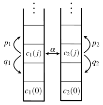
Our model consists of two vertical, semi-infinite discrete columns, with sites at height $i$ having concentrations $c_{1}(i,n)$ and $c_{2}(i,n)$, respectively, at time step $n$; see Fig. 1. Reflecting boundaries are placed at the bottom of each column, which we take to be at $i=0$. In each column $\nu=1,2$, we consider biased random walkers in discrete time, with probabilities ${p}_{\nu}$ to jump upwards and ${q}_{\nu}=1-{p}_{\nu}$ to jump downwards at each time step. To enforce the reflecting boundary condition, walkers which try to jump downwards from site $0$ remain at site $0$. We believe that this is the simplest model in which the effect is found, allowing a complete analytical solution. However, as we discuss below, similar phenomena can be expected to arise whenever two or more systems with spatially varying equilibrium states are coupled at several places.

Figure 1: Transition probabilities between sites and stationary occupation probabilities.

When the columns are not coupled, the following master equation describes the time evolution of the concentrations:

$$c_{\nu}(i,n+1)={p}_{\nu}c_{\nu}(i-1,n)+{q}_{\nu}c_{\nu}(i+1,n),\quad j\neq 0$$ (1)

with boundary conditions

$$c_{\nu}(0,n+1)={q}_{\nu}c_{\nu}(0,n)+{q}_{\nu}c_{\nu}(1,n).$$ (2)

If ${q}_{\nu}\geq{p}_{\nu}$, i.e., if the bias is directed towards the reflecting boundary at the origin, then the physical (i.e., normalizable) stationary solutions of these equations are:

$$c_{\nu}(i)={K}_{\nu}\left({p}_{\nu}/{q}_{\nu}\right)^{i},$$ (3)

where the ${K}_{\nu}$ are normalization constants. The crucial feature of these solutions is that the vertical current $J_{\nu}(i):={p}_{\nu}c_{\nu}(i-1)-{q}_{\nu}c_{\nu}(i)$ between sites within either column vanishes identically, so that the system is in equilibrium.

2.2 Coupling

We now couple the columns together so that they may exchange particles at a single height $j$, where particles have the same probability $\alpha$ to jump “horizontally” from one column to the other in either direction (see Fig. 1). The equations describing the system are then modified in the vicinity of site $j$ to take account of the additional current due to the coupling:

$$c_{\nu}(j+1,n+1)=(1-\alpha){p}_{\nu}c_{\nu}(j,n)+{q}_{\nu}c_{\nu}(j+2,n);$$

$$c_{\nu}(j-1,n+1)={p}_{\nu}c_{\nu}(j-2,n)+(1-\alpha){q}_{\nu}c_{\nu}(j,n);$$

$$c_{1}(j,n+1)={p}_{1}c_{1}(j-1,n)+{q}_{1}c_{1}(j+1,n)+\alpha c_{2}(j,n);$$

$$c_{2}(j,n+1)={p}_{2}c_{2}(j-1,n)+{q}_{2}c_{2}(j+1,n)+\alpha c_{1}(j,n).$$

There is then a unique stationary solution for the whole system, given by

$$c_{\nu}(i)=K\cases{(1-\alpha)\left({p}_{\nu}/{q}_{\nu}\right)^{i-j}&if $i\neq j$;\\ 1&if $i=j$,}$$ (4)

for $\nu=1,2$, with a single normalization constant $K$. Note that the concentrations in the two sites at height $j$, where interchange is allowed, are equal, giving a zero total horizontal current there. Thus, this is again an equilibrium distribution with vanishing current everywhere, showing that such a coupling procedure is natural, and allows the systems to equilibrate with each other.

3 Non-equilibrium stationary state

However, coupling at more than one site instead forces the system to settle into a nonequilibrium stationary state, with non-vanishing currents. To show this, in what follows we consider the case of horizontal coupling at every height, with symmetrical probability $\alpha$ of jumping between columns.

In the stationary state, the concentrations satisfy the following set of coupled linear equations at sites $i\neq 0$:

$$c_{1}(i)=\left(1-\alpha\right)\left[{p}_{1}c_{1}(i-1)+{q}_{1}c_{1}(i+1)\right]+\alpha c_{2}(i),$$ (5)

$$c_{2}(i)=\left(1-\alpha\right)\left[{p}_{2}c_{2}(i-1)+{q}_{2}c_{2}(i+1)\right]+\alpha c_{1}(i).$$ (6)

At height $0$, the reflecting boundary conditions give the following:

$$c_{1}(0)=\left(1-\alpha\right)\left[{q}_{1}c_{1}(0)+{q}_{1}c_{1}(1)\right]+\alpha c_{2}(0),$$ (7)

$$c_{2}(0)=\left(1-\alpha\right)\left[{q}_{2}c_{2}(0)+{q}_{2}c_{2}(1)\right]+\alpha c_{1}(0).$$ (8)

To solve the system (5)–(8), we introduce generating functions [8], a discrete version of the Laplace transform:

$$\hat{C}_{\nu}(z):=\sum_{i=0}^{\infty}c_{\nu}(i)z^{i},\qquad\nu=1,2.$$ (9)

Multiplying (5) and (6) by $z^{i}$, summing over $i$ from $1$ to $\infty$, and using the boundary conditions leads to two simultaneous linear equations for the generating functions in terms of the values of the concentrations $c_{1}(0)$ and $c_{2}(0)$ at the boundary, which have yet to be determined:

$$\left(\begin{array}[]{cc}f_{1}(z)&-\alpha\\ -\alpha&f_{2}(z)\end{array}\right)\left(\begin{array}[]{c}\hat{C}_{1}(z)\\ \hat{C}_{2}(z)\end{array}\right)=\left(\begin{array}[]{c}g_{1}(z)\\ g_{2}(z)\end{array}\right),$$ (10)

where $f_{\nu}(z):=1-(1-\alpha)[{p}_{\nu}z+\frac{{q}_{\nu}}{z}]$ and $g_{\nu}(z):=(1-\alpha){q}_{\nu}(1-\frac{1}{z})c_{\nu}(0)$.

Solving yields

$$\hat{C}_{1}(z)=\frac{[z-(1-\alpha)({p}_{2}z^{2}+{q}_{2})]{q}_{1}c_{1}(0)+\alpha z{q}_{2}c_{2}(0)}{\alpha z\left[{q}_{1}+{q}_{2}-z({p}_{1}+{p}_{2})\right]-(1-\alpha)(1-z)({q}_{1}-z{p}_{1})({q}_{2}-z{p}_{2})},$$ (11)

and an analogous equation for $\hat{C}_{2}(z)$ with the subscripts $1$ and $2$ interchanged in the numerator (the denominator being unchanged). This gives (in principle) an exact solution for the stationary concentration distributions, obtained by inverting Eq. (9): $c_{\nu}(i)=\frac{1}{i!}\hat{C}^{(i)}_{\nu}(0)$, where $\hat{C}_{\nu}^{(i)}$ denotes the $i$th derivative; or, equivalently, by expanding in formal power series in $z$ and equating coefficients.

The vertical current in column $\nu$ between site $j$ and site $j+1$ is given by $J_{\nu}(j):=(1-\alpha)[{p}_{\nu}c_{\nu}(j)-{q}_{\nu}c_{\nu}(j+1)]$. The corresponding generating functions follow from Eq. (11):

$$\hat{J}_{1}(z)=\alpha(1-\alpha)\frac{({q}_{2}-z{p}_{2}){q}_{1}c_{1}(0)-({q}_{1}-z{p}_{1}){q}_{2}c_{2}(0)}{\alpha z\left[{q}_{1}+{q}_{2}-z({p}_{1}+{p}_{2})\right]-(1-z)(1-\alpha)[{q}_{1}-z{p}_{1}][{q}_{2}-z{p}_{2}]}$$ (12)

and $\hat{J}_{2}(z)=-\hat{J}_{1}(z)$, reflecting the fact that the system is in a steady state. However, neither current (in either column) can be identically zero unless the corresponding hopping probabilities are equal, $p_{1}=p_{2}$, in which case the steady state is an equilibrium state. Rather, there is a circulation through the system, moving upwards in the column with larger $p_{\nu}$ and downwards in the other column.

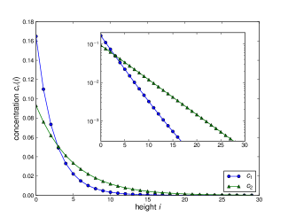
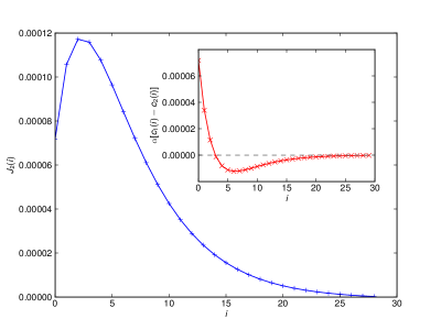
Figures 2 and 3 show this phenomenon for a representative set of parameters, giving the concentration profiles, and vertical and horizontal current, respectively. The stationary solution was obtained by numerically iterating the master equation for the time evolution of the $c_{\nu}(i)$, using a finite system with a reflecting boundary condition also at the top, confirming that the concentration profiles have exponential tails. It may be checked that this numerical solution agrees with the exact solution described below when the corresponding parameter values are substituted in the exact expressions.

Figure 2: Steady-state concentrations $c_{\nu}(i)$ as a function of height $i$ with coupling at all heights; the lines are a guide for the eye. Parameters: $p_{1}=0.4$; $p_{2}=0.45$; $\alpha=0.001$; system height $N=30$ with upper and lower reflecting boundary conditions. Inset: same data on a semi-logarithmic scale.

Figure 3: Vertical current $J_{2}(i)$ as a function of height $i$; same parameters as in Fig. 2. Inset: horizontal current as a function of height.

Other relevant quantities can also be easily calculated. For example, since there is a sustained current in the system, it must be driven by thermodynamic forces. These forces can be related to the respective hopping probabilities ${p}_{\nu}$ and ${q}_{\nu}$ in each column via $f_{\nu}=\ln({p}_{\nu}/{q}_{\nu})$; this identification arises from the fact that when $\alpha=0$, the concentrations reach equilibrium distributions of the form $c_{\nu}(j){\sim}({p}_{\nu}/{q}_{\nu})^{j}=\exp[-j\,\ln({q}_{\nu}/{p}_{\nu})]$, so that $j\,\ln({q}_{\nu}/{p}_{\nu})$ is a potential from which the force $f_{\nu}$ is derived. Then, the amount of “work” dissipated can be calculated from the generating function $\hat{W}(z)=\ln({p}_{1}/{q}_{1})\hat{J}_{1}(z)+\ln({p}_{2}/{q}_{2})\hat{J}_{2}(z)$, giving that the total work dissipated within the system is

$$\hat{W}(z=1)=(1-\alpha)\left[\ln({q}_{2}{p}_{1}/{p}_{2}{q}_{1})\right]\frac{\left[({q}_{2}-{p}_{2}){q}_{1}c_{1}(0)-({q}_{1}-{p}_{1}){q}_{2}c_{2}(0)\right]}{\left[{q}_{1}+{q}_{2}-({p}_{1}+{p}_{2})\right]}.$$ (13)

4 Exact solution and asymptotics

To evaluate and make use of all of the above analytical expressions, we must determine the hitherto unknown constants $c_{1}(0)$ and $c_{2}(0)$. Taking the limit $z\to 1$ in Eq. (11) gives $\lim_{z\to 1}\hat{C}_{1}(z)=\lim_{z\to 1}\hat{C}_{2}(z)$, i.e., the total probabilities in each column are equal in the stationary state. This is a result of the nature of the coupling used, and expresses the fact that the total current from one column to the other must be $0$ in the stationary state. (Note that the (horizontal) current from one column to the other, at height $i$, is $\alpha[c_{1}(i)-c_{2}(i)]$.)

In what follows, we assume the total normalization to be equal to one, so that $\hat{C}_{1}(z=1)=\hat{C}_{2}(z=1)=\frac{1}{2}$. Evaluating this equality gives one relation between the unknown constants $c_{1}(0)$ and $c_{2}(0)$:

$${q}_{1}c_{1}(0)+{q}_{2}c_{2}(0)=1-(p_{1}+p_{2})={q}_{1}-{p}_{2}.$$ (14)

To determine another relation between them, and hence find their precise values, we use the face that the generating functions $\hat{C}_{\nu}$ be analytic in the region $|z|\leq 1$ [12]. Indeed, $c_{\nu}(j)$ are probabilities, and thus take values in the interval $[0,1]$, so that generating functions $\hat{C}_{\nu}(z)$ can have no poles in the interval $z\in[0,1]$.

To impose this constraint, we must determine the zeros of the denominator $\Delta(z)$ in the expression (11) for the $\hat{C}_{\nu}(z)$, given by

$$\Delta(z):=\alpha z\left[{q}_{1}+{q}_{2}-z({p}_{1}+{p}_{2})\right]-(1-z)(1-\alpha)({q}_{1}-z{p}_{1})({q}_{2}-z{p}_{2}).$$ (15)

Since $\Delta(0)=-{q}_{1}{q}_{2}(1-\alpha)<0$ and $\Delta(1)=2\alpha({q}_{1}+{q}_{2}-1)$, a sufficient condition for $\Delta(z)$ to have a zero in the interval $(0,1)$ is that ${q}_{1}+{q}_{2}>1$. We denote the zeros of $\Delta$ by $z_{0}\in(0,1)$ and $z_{1},z_{2}\geq 1$. For $\hat{C}_{1}(z)$ and $\hat{C}_{2}(z)$ to have no poles in $(0,1)$, the numerator in Eq. (11) must thus also vanish at $z_{0}$.

Since $\Delta(z)$ is a cubic polynomial, one can find exact explicit expressions for $z_{0}$ in terms of the parameters of the system. However, the general resulting expressions are cumbersome and unenlightening, and we do not give them here.

Nonetheless, simple perturbative expressions can be found, for example, in the limit of small $\alpha$, for which we have, to first order in $\alpha$,

$$z_{0}\simeq 1-\alpha\frac{({q}_{1}+{q}_{2})-({p}_{1}+{p}_{2})}{({q}_{1}-{p}_{1})({q}_{2}-{p}_{2})},$$ (16)

provided ${q}_{1}>{p}_{1}$ and ${q}_{2}>{p}_{2}$. If, instead, ${p}_{1}>{q}_{1}$, say, and ${q}_{2}$ is large enough to ensure that $\Delta(1)>0$, then to first order

$$z_{0}\simeq\frac{{q}_{1}}{{p}_{1}}-\alpha\frac{{q}_{1}}{{p}_{1}-{q}_{1}},$$ (17)

whereas if ${q}_{1}={p}_{1}$ then $z_{0}\simeq 1-\sqrt{2\alpha}$.

Imposing the condition of analyticity on, say, $\hat{C}_{1}(z)$ then provides the missing condition to determine $c_{1}(0)$ and $c_{2}(0)$:

$$[z_{0}-(1-\alpha)({p}_{2}z_{0}^{2}+{q}_{2})]{q}_{1}c_{1}(0)+\alpha{q}_{2}c_{2}(0)=0.$$ (18)

Note that, given the form of the denominator, had we chosen instead to impose the requirement of analyticity at $z_{0}$ on $\hat{C}_{2}(z)$, we would have arrived at the same condition. Equivalently, we could impose that the generating function for the current, Eq. (12), be analytic at $z_{0}$. This leads to

$$c_{1}(0)=\frac{1}{2}\left[\frac{({q}_{1}+{q}_{2})-({p}_{1}+{p}_{2})}{({q}_{1}+{q}_{2})-z_{0}({p}_{1}+{p}_{2})}\right]({q}_{1}-z_{0}{p}_{1})$$ (19)

and a corresponding equation for $c_{2}(0)$, which provide the complete solution to the problem in terms of the root $z_{0}$. Then, for example, substitution of these expressions in the equation for the total work dissipated in the system gives

$$\hat{W}(z=1)=\frac{\alpha z_{0}}{2}\left[\frac{{p}_{1}{q}_{2}-{p}_{2}{q}_{1}}{({q}_{1}-z_{0}{p}_{1})({q}_{2}-z_{0}{p}_{2})}\right]\ln\left(\frac{{q}_{2}{p}_{1}}{{q}_{1}{p}_{2}}\right).$$

The generating functions $\hat{C}_{\nu}(z)$ of the concentrations, as shown in Eq. (11), are rational functions of $z$, which correspond to concentration profiles formed by a linear combination of decaying exponentials $z_{1}^{-j}$ and $z_{2}^{-j}$. As is the case for $z_{0}$, approximate expressions for these other roots at small values of $\alpha$ can easily be calculated. For example, when ${p}_{1}<{q}_{1}$ and ${p}_{2}<{q}_{2}$, to first order in $\alpha$ we have

$$z_{\nu}\simeq\frac{{q}_{\nu}}{{p}_{\nu}}+\alpha\frac{{q}_{\nu}}{{q}_{\nu}-{p}_{\nu}},\qquad\nu=1,2.$$ (20)

A special case occurs when one of the ${p}_{\nu}$ vanishes, say $p_{2}=0$. In this case, the cubic denominator $\Delta(z)$ simplifies to a quadratic, and the exact expressions for its zeros become significantly simpler:

$$z_{0,1}=\frac{1+\alpha q_{1}\pm\sqrt{(1+\alpha q_{1})^{2}-4p_{1}q_{1}(1-\alpha)}}{2p_{1}},$$ (21)

where $z_{0}\in[0,1]$ is given by taking the minus sign for the radical. The $\hat{C}_{\nu}(z)$ must vanish at $z=z_{0}$, giving a single factor $z-z_{1}$ in the denominator. The two concentration profiles are then exactly exponential for $i>0$, differing only by a multiplicative factor and the concentration at height $0$.

5 Conclusions

Figure 4: Concentration profiles $c_{\nu}(i)$ (shown on a semi-logarithmic scale) as a function of height $i$ when the horizontal coupling is allowed only at two heights, $j_{1}=6$ and $j_{2}=14$; vertical dashed lines indicate the different regimes. Parameters: $p_{1}=0.4$, $p_{2}=0.45$, $\alpha=0.1$, $N=30$. Inset: Vertical current $J_{2}(i)$, which is constant between $j_{1}$ and $j_{2}$, as it must be.

In conclusion, by furnishing a complete analytical solution, we have shown that coupling together two simple biased diffusive systems can give rise to nonequilibrium steady state with a sustained current throughout the combined system, even though each of them separately reaches equilibrium. This effect arises due to the fact that the equilibrium profiles can be “matched” when the systems are coupled at just a single site, so that the current across that site vanishes, whereas if the coupling occurs at various sites, then the equilibrium distributions can no longer be made to match at all sites simultaneously.

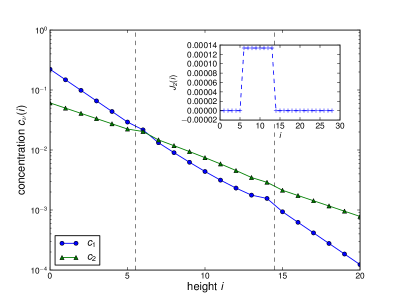
The same phenomenon thus occurs even with coupling at only two heights, $j_{1}$ and $j_{2}$. The density profiles and currents obtained numerically for a specific realization of this minimal case are shown in Fig. 4. This case can also be solved analytically: below $j_{1}$ and above $j_{2}$, the profiles are exactly exponential, due to the absence of current there; these exponentials are matched with the exact solution between $j_{1}$ and $j_{2}$.

Physical realizations of this phenomenon may be obtained, for example, with particles suspended in a fluid under the combined effect of gravity and an applied electric field, as in electrophoresis. If the particles are capable of capturing or losing a charge (or can be induced to do so), then they can transition from one charge state to the other. The drift induced by the field will then differ depending on the charge state of the particle. Note that our model can also be interpreted in this way, where the subindex describes the charge state of the particle, rather than its physical position.

These and other realizations may require generalizing the analysis to the case in which there is asymmetric coupling, i.e., in which the probability of jumping from state 1 to state 2 differs from the reverse transition probability. The effect described in this work will nonetheless persist.

Financial support from SEP-CONACYT grant CB-101246 and PAPIIT grants IN109111, IN116212 and IN117214 from DGAPA-UNAM is acknowledged.

Bibliography

- [1] M. Jean Perrin. Brownian Movement and Molecular Reality. Taylor and Francis, London, 1910.
- [2] S. Chandrasekhar. Stochastic problems in physics and astronomy. Rev. Mod. Phys., 15:1–89, Jan 1943.
- [3] M.C. Wang and G.E. Uhlenbeck. On the theory of the Brownian motion II. Rev. Mod Phys, 17:323–342, 1945.
- [4] T. Biben, J.P. Hansen, and J. L. Barrat. Density profiles of concentrated colloidal suspensions in sedimentation equilibrium. J. Chem. Phys., 98:7739, 1993.
- [5] E. Bringuier. From mechanical motion to Brownian motion, thermodynamics and particle transport theory. Eur. J. Phys., 29:1243–1262, 2008.
- [6] Xue-Juan Zhang, Hong Qian, and Min Qian. Stochastic theory of nonequilibrium steady states and its applications. part I. Phys. Rep., 510(1–2):1–86, 2012.
- [7] M. Kac. Random walk and the theory of Brownian motion. Amer. Math. Monthly, 54(369–391), 1947.
- [8] G.H. Weiss. Aspects and Applications of the Random Walk. North-Holland, Amsterdam, 1994.
- [9] Anatoly B. Kolomeisky. Exact results for parallel-chain kinetic models of biological transport. J. Chem. Phys., 115(15):7253–7259, 2001.
- [10] Evgeny B. Stukalin and Anatoly B. Kolomeisky. Transport of single molecules along the periodic parallel lattices with coupling. J. Chem. Phys., 124(20):204901, 2006.
- [11] Hamid Teimouri and Anatoly B. Kolomeisky. All-time dynamics of continuous-time random walks on complex networks. J. Chem. Phys., 138(8):084110, 2013.
- [12] R. Rajesh and S.N. Majumdar. Exact calculation of the spatiotemporal correlations in the Takayasu model and in the -model of force fluctuations in bead packs. Phys. Rev. E, 62(3186–3196), 2000.