From mobile phone data to the spatial structure of cities

Abstract

Pervasive infrastructures, such as cell phone networks, enable to capture large amounts of human behavioral data but also provide information about the structure of cities and their dynamical properties. In this article, we focus on these last aspects by studying phone data recorded during 55 days in 31 Spanish metropolitan areas. We first define an urban dilatation index which measures how the average distance between individuals evolves during the day, allowing us to highlight different types of city structure. We then focus on hotspots, the most crowded places in the city. We propose a parameter free method to detect them and to test the robustness of our results. The number of these hotspots scales sublinearly with the population size, a result in agreement with previous theoretical arguments and measures on employment datasets. We study the lifetime of these hotspots and show in particular that the hierarchy of permanent ones, which constitute the ‘heart’ of the city, is very stable whatever the size of the city. The spatial structure of these hotspots is also of interest and allows us to distinguish different categories of cities, from monocentric and ”segregated” where the spatial distribution is very dependent on land use, to polycentric where the spatial mixing between land uses is much more important. These results point towards the possibility of a new, quantitative classification of cities using high resolution spatio-temporal data.

Introduction

Pervasive, geolocalized data generated by individuals has recently triggered a renewed interest for the study of cities and urban dynamics, and in particular, individual mobility patterns Asgari2013 . Various data sources have been used such as car GPS gallotti_towards_2012 ; Furletti2013 , RFIDs for collective transportation roth2011structure , and also data coming from social networks such as TwitterHawelka2013 or Foursquarenoulas_tale_2012 . A recent, very important source of data is given by individual mobile phone data onnela2007structure ; lambiotte2008geographical . These data have allowed to study the individual mobility patterns with a high spatial and temporal resolution gonzalez2008understanding ; schneider2013unravelling ; kung_exploring_2013 , the automatic detection of urban land uses pei_new_2013 , or the detection of communities based on human interactions sobolevsky_delineating_2013 .

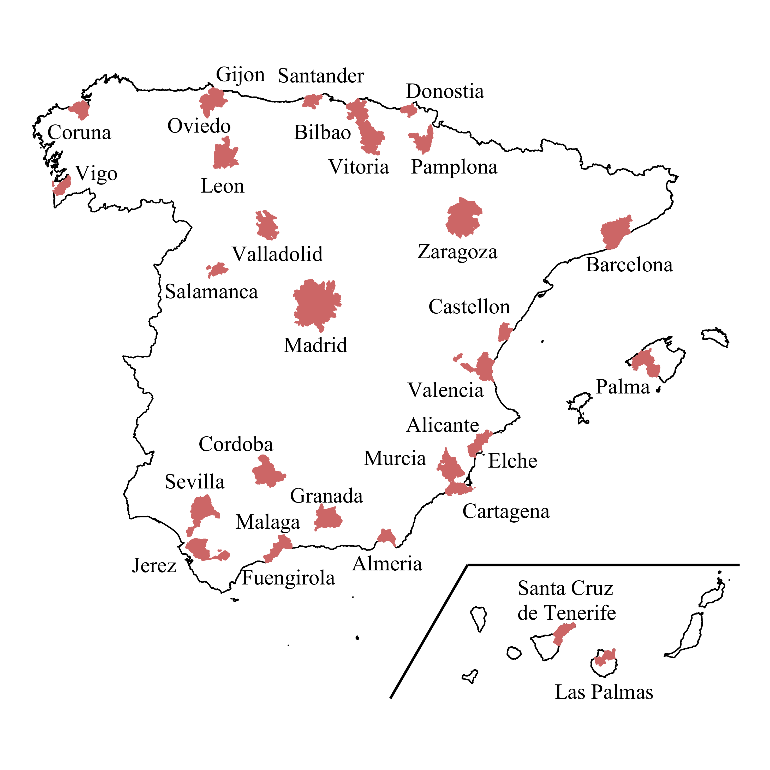
Morphological aspects, such as the quantitative characterization and comparison of cities through their density landscape, their space consumption, their degree of polycentrism, or the clustering degree of their activity centers, have been studied for a long time in quantitative geography and spatial economy anas_urban_1997 ; bertaud2003spatial ; Tsai2005 ; pereira_urban_2013 ; schwarz2010 ; thomas_morphology_2008 ; Guerois2008 ; berroir2011 ; LeNechet2012 . Until the late 2000, these quantitative comparisons of cities were necessarily based on census data and/or remote sensing data, both giving a static estimation of the density of individuals and land uses in the city, at a fine spatial granularity but at a fixed, unique point in time. Given the atemporal nature of these studies, they could not investigate some interesting questions related to the dynamical properties of the spatial structure of cities: how much does the city shape change through the course of the day? Where are the city’s hotspots located at different hours of the day? How are these hotspots spatially organized? Is there some kind of typical distance(s) characterizing the permanent core, or ‘backbone’, of each city? Mobile phone data contain the spatial information about individuals and how it evolves during the day. These datasets thus give us the opportunity to answer some of these questions and to characterize quantitatively the spatial structure of cities. In this article, we address some of these questions using mobile phone data for a set of $31$ Spanish cities shown on Figure 1.

Figure 1: The 31 Spanish cities (urban areas) with more than 200,000 inhabitants in 2011. Map of their locations and spatial extensions. The set of cities analyzed in this article comprises very different types of cities such as central cities, port cities and cities on islands.

We focus on the spatio-temporal properties of cities and, defining new metrics, study their structural properties and exhibit interesting patterns of urban systems.

Results

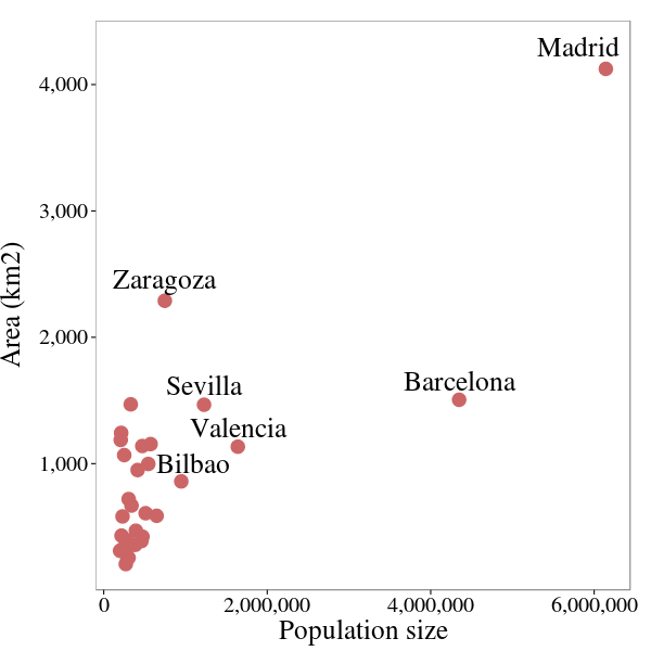
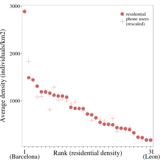
Our analysis is based on aggregated and annonymized mobile phone traces provided by a Spanish telecommunications operator, which concerns 31 Spanish urban areas studied during weekdays. These urban areas are very diverse in terms of geographical location, area, population size and density, as illustrated by Figure 2. In particular, the wide range of population sizes will allow us to test some scaling relations and also to identify various behaviors. We will first describe the dataset and then present the results obtained about several aspects of cities.

(a)	(b)

a

Figure 2: Population sizes, areas and densities of 31 Spanish cities (urban areas) with more than 200,000 inhabitants in 2011. (a) Population size vs. area. The set of cities under study displays a large variety of sizes. We also note that there is no general statistical relation between the population size of Spanish urban areas and their spatial extension. (b) Rank-size distribution of their residential density and phone activity density (rescaled by a constant factor given by the inverse of the fraction of phone users in the denser urban area, $\rho_{Barcelona,residential}/\rho_{Barcelona,phoneusers}$). The distribution shows that the fraction of phone users is almost constant in all cities.

Data description

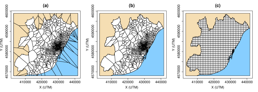
Our analysis is based on a mobile phone dataset provided by a Spanish telecommunications operator. The aggregated records represent the number of unique individuals using a given antenna for each hour of the day. No individual information or records were available for this study. These data provide some snapshots of the spatial distribution of people in the city at successive points in time. We have this information for the 31 Spanish urban areas of more than 200,000 inhabitants, and for 55 days. The number of users (per hour) represents in average $2\%$ of the total population and at most $5\%$ of the total population. These percentages are almost the same for all the urban areas. Given the irregularity of the spatial distribution of the antennas in each city and from one city to another, we spatially aggregated the number/densities of users recorded each hour in each mobile phone antenna on a regular square grid of varying cell size $a$, in order to simplify comparisons of indicators between cities, as shown on Figure 3. The choice of the spatial scale of data aggregation is known to be an important source of bias in spatial analysis openshaw1979million , hence we tested the robustness of our results on three different sizes of grid cells (see section Methods for details).

Figure 3: Map of the metropolitan area of Barcelona. The white area represents the metropolitan area, the brown area represents territories surrounding the metropolitan area and the blue area the sea. (a) Voronoi cells of the mobile phone antennas point pattern. (b) Intersection between the Voronoi cells and the metropolitan area. (c) Grid composed of 1 km² square cells on which are aggregated the number/density of unique phone users associated to each phone antenna.

General features

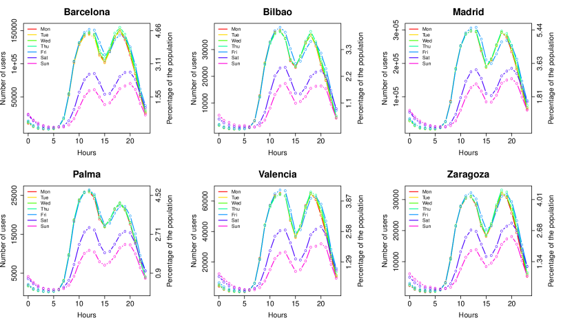
In order to get a preliminary grasp of the data we plot the time evolution of the number of users along the day and see if it follows the same pattern in every city. Figure 4 shows the average number of mobile phone users per hour according to the day of the week for six of them. Globally, the number of phone users is significantly higher during the weekdays than during the weekends, except at night time. From 11pm to 8am, the number of users is relatively low, it reaches a minimum at 5am during weekdays and at 7am during the weekend. For all cities we observe two activity peaks, one at 12am during weekdays (1pm during the weekend) and another one at 6pm during weekdays (and at 8pm during the weekend).

Figure 4: Number of mobile phone users according to the hour of the day, for each day of the week, in six Spanish metropolitan areas.

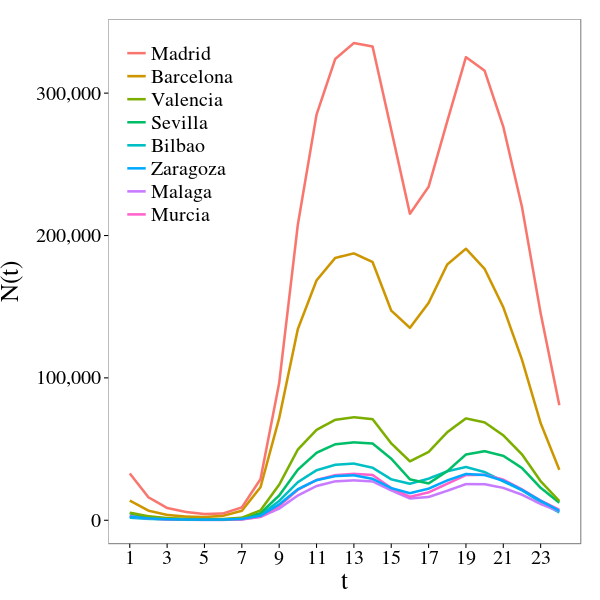
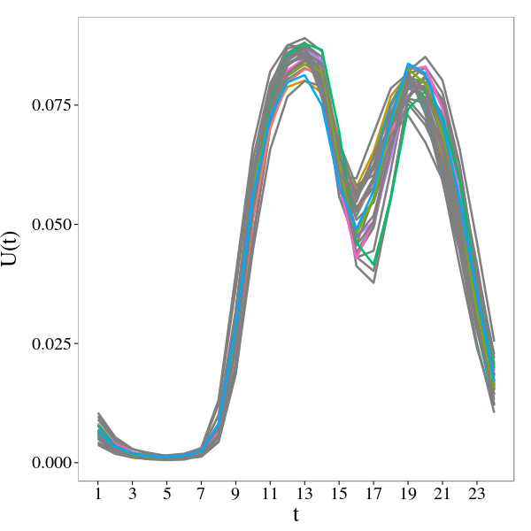
In order to compare these values obtained for different cities, we rescale the values by the total number of users for an average weekday. We show the results in Figure 5. The rescaled plot suggests the existence of a single ‘urban rhythm’ common to all cities. The data collapse is very good in the morning, while in the afternoon we observe a little more variability from one city to another. It is interesting to note that in four cities located in the western part of Andalusia (Sevilla, Granada, Cordoba and Jerez de la Frontera) the activity restarts later in the afternoon, around 5pm one hour later than in the other cities.

(a)	(b)

Figure 5: Time evolution of the number of mobile phone users per hour during an average weekday (a) Total number of unique mobile phone users per hour (shown here for the eight biggest Spanish cities). (b) Rescaled numbers of unique users per hour for 31 cities. Each value $U_{i}(t)$ is equal to the number of phone users in city $i$ at time $t$, $N_{i}(t)$, divided by the total number of phone users in $i$ during the entire day : $U_{i}(t)=N_{i}(t)/\sum_{t=1}^{t=24}N_{i}(t)$. The good collapse suggests the existence of an urban rhythm common to all cities.

Global weighted indicators versus hotspots analysis

Essentially, the mobile phone data give access to the local density $\rho(i,t)$ of users at a location $i$ and at a time $t$. The difficulty is then to study this complex object which displays variation in time and space. We will consider here two main directions to tackle this problem. The first one is to define global indicators that consider all points and weight them by the user density. The second approach consists in identifying local maxima of the function $\rho(i,t)$, or in other words, the hotspots. There are pros and cons in each method. Looking at hotspots is convenient since it provides a clear picture of the important locations in the city, but contains some arbitrariness in their determination. On the other hand, working with weighted indices does not require to identify hotspots but at the cost of producing results more difficult to interpret. These two approaches can however be seen as complementary since they highlight different properties of the city: weighted indices inform us about the global properties of a given city, while the hotspots give us a more local look and allow us to concentrate on the ‘heart’ of the city. This is why in the following we will successively apply the two methods.

Global analysis

Urban dilatation index

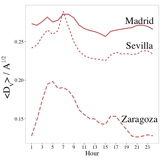
The average weighted distance $D_{V}(t)$ between individuals in the city (see section Methods for the precise definition) and its evolution during the course of an average weekday provides a first interesting indicator about the organization of the city. Figure 6 (a) shows the evolution of this normalized average, weighted distance during a typical weekday.

(a)	(b)

Figure 6: Time evolution of the average distance $D_{V}(t)$ between phone users in the city, and the values of the dilatation index $\mu=\max D_{V}(t)/\min D_{V}(t)$ for the 31 Spanish metropolitan areas studied. (a) Illustration of the time evolution of $D_{V}$ in three urban areas: Madrid, Sevilla and Zaragoza. This distance $D_{V}$ is equal to the average of the distances between each pair of cells weighted by the density of each of the cells. The resulting distance is then divided by the typical spatial size of the city (given by $\sqrt{A}$ the square root of the city’s area) in order to compare the curves across cities. (b) Rank-size distribution of the dilatation index $\mu$ in the 31 metropolitan areas.

We can essentially distinguish two broad categories according to the spatial organization of residences and activities:

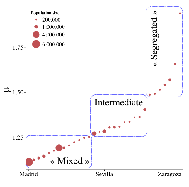
• In the case of the simple picture of a typical monocentric city with predominant Central Business District (CBD), the city collapses in the morning when people living in the suburbs commute to their workplaces, and expands in the evening when they get back home. We then expect in this case a large variation (at the city scale) of the average distance $D_{V}$. In this case, activity and residential places are spatially ”segregated”.

• For more polycentric cities, where residential and work places are spatially less separated, we expect a smaller variation of $D_{V}$ than the one observed for monocentric cities. Here activity places and residential areas are more ”mixed”.

For all cities we observe the same typical pattern: we see two peaks, one around 7 am, when people switch on their mobile phones, probably at home or when they are in transportation system’s entry points (see Figure 6(a)). We then see a decrease of the distance (the city ‘collapses’), displaying spatial concentration of individuals during the middle of the day, mainly corresponding to the activity period for most individuals (workers/students). During the afternoon we see a second, smaller peak dispersed over 4-5pm, when people start going back home. This afternoon peak is less pronounced, suggesting a higher variety of mobility behaviors at the end of the day. The interesting feature of theses curves is the variation amplitude that informs us about the importance of this collapse phenomenon. Despite the fact that several factors such as phone use or behavioral factors affect these variations, we observe a common pattern: a pronounced peak at the beginning of the day and a minimum usually observed at the middle of the day. From this curve it is then natural to calculate for each city a ‘dilatation coefficient’ defined as

$$\mu=\frac{\max_{t}(D_{V}(t))}{\min_{t}(D_{V}(t))}$$ (1)

We show in Figure 6(b) the rank plot of this dilatation index obtained for the 31 cities where we can distinguish roughly three groups of cities. For the first group with a value of $\mu$ around one, the average distance stays approximately constant throughout the day. This means that whatever the hour of the day, the spatial spread of the high density locations does not change significantly. High density locations correspond to different activities depending on the moment of the day, and a small value of the dilatation coefficient implies that daytime activity places (work places, schools, leisure places) are not more spatially concentrated than residences. Homes and activity places are more entangled, supporting the picture of more ‘mixed’ cities, such as Madrid for example. In the opposite case of large values, the spatial organization of the different high-density locations changes significantly along the day. A typical example would be a monocentric city where individuals are localized in the CBD during the day and where residences are spread all around the center. In our set, Zaragoza for example is representative of this type of cities. For the intermediate group the cities display a less marked behavior, probably resulting of a combination of monocentric and polycentric features.

Hotspots analysis

Identifying the hotspots

This problem corresponds to identify local maxima in the surface of density of users. A simple method amounts to choose a threshold $\delta$ and to consider that every point $i$ with a density larger than this threshold $\rho(i,t)>\delta$ is a hotspot at time $t$. Most of the methods so far rely on this simple argument but there is obviously some arbitrariness in the choice of $\delta$. In contrast here (all technical details can be found in the Methods section), we discuss two extreme choices for the threshold value. The lower threshold $\delta_{min}$ corresponds to the average value of the density, which is indeed a reasonable, minimal requirement to be a local maxima. Based on considerations about the Lorenz curve of the density, we are also able to determine another value $\delta_{max}$ which can be considered as the maximal, reasonable value for $\delta$. In the following we will distinguish the ‘Average’ method from the ‘Loubar’ method which correspond to the two values $\delta_{min}$ and $\delta_{max}$, respectively. The most important point here, is that once the lower and upper bounds for the threshold are determined and allow for the identification of hotspots, all the results obtained should be robust with respect to the choice of $\delta$. In other words, if a given result is qualitatively the same when considering the lower and upper bounds for $\delta$, the result can safely be considered as an intrinsic feature of the system.

Number of hotspots

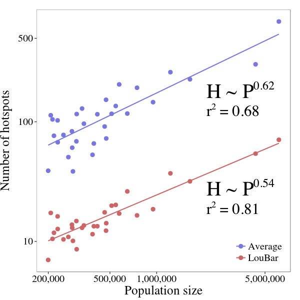
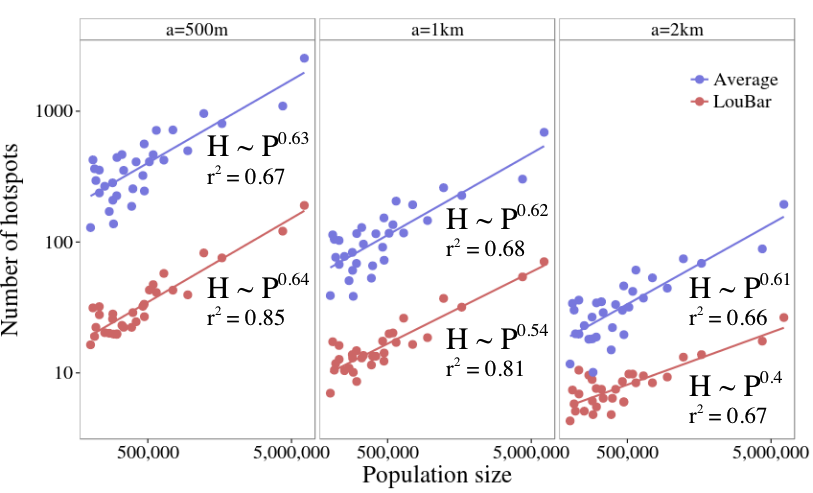
We first focus on the number of hotspots. Using both methods, ’Average’ and ‘Loubar’, for each city we count the number of hotspots at each hour of the day, compute the average over the day and see how this average number scales with the population size of the city. This measure is motivated by recent theoretical and empirical work LoufBarthelemy2013 that has highlighted a clear sub-linear relation between the population size of cities and their number of activity centers (defined as employment hotspots). For the U.S., it has been shown that the number of activity centers $N_{a}$ (determined from employment data) scales as

$$N_{a}\sim P^{\beta}$$ (2)

with $\beta\sim 0.64$. Figure 7 displays the number $H$ of hotspots versus the population for the set of the 31 biggest Spanish cities considered here. The power law fit confirms the result obtained in LoufBarthelemy2013 that there is a sublinear relation and, remarkably enough, that the value of the exponent is of the same order. We note here that this result is robust against the thresholding criteria used to define hotspots (see also section Methods for aggregation grids with different cell sizes).

Figure 7: Scatter plot and fit of the number of hotspots $H$ vs. the population size $P$ for the 31 cities studied. Each point in the scatterplot corresponds to the average number of hotspots determined for each one-hour time bin of a weekday (for five weekdays considered here). The power law fit is consistent, for both hotspots identification methods, with a sublinear behavior characterized by an exponent of order $0.6$, a value in agreement with theoretical predictions and empirical observations on employment data LoufBarthelemy2013 .

We also note here that recent empirical work arcaute_city_2013 has highlighted the sensitivity of the values of scaling laws exponents to the choice of city boundaries. This result underlines the crucial role of city definition when attempting to identify patterns of behavior across cities, and the need for consistency in defining the spatial boundaries of cities for such comparisons bretagnolle_organisation_2009 . That is the reason that has led us to rely on the spatial delimitations of urban areas, which are harmonized delimitations based on the ratio of home-work commuting journeys (see Methods for details).

Stability of the hotspots hierarchy

Another interesting feature to inspect in cities is the stability of their hotspots and the evolution of their relative importance in the city according to the hour of the day, which is related to the evolution of the hierarchy of places in the city. In order to capture the behavior of cities about these aspects, we plot various indicators. We start with the histogram of the persistence of hotspots: for each city we count the number of one-hour time bins during which each cell has been a hotspot. We then plot the distribution of the hotspots ‘lifetime’ (measured in number of one-hour bins), as shown in Figure 8 for the eight largest Spanish cities.

Figure 8: Histogram of lifetime duration of hotstpots for eight cities and for the two hotspots identification methods (top: ‘Average’ method and bottom: ‘Loubar’ method). In the case of the ’Loubar’ hotspots, we can essentially distinguish three groups: the permanent (24h hotspots), intermittent (from 1 up to 7 hours) and intermediary (all the others) hotspots.

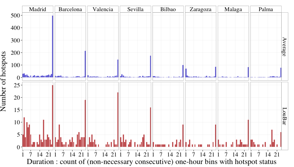
Figure 8 highlights the importance of ‘permanent’ hotspots, i.e. locations which are hotspots during the whole day. Each city has its number of important locations, those that form the ‘heart’ of the city. In addition to the permanent hotspots we also observe two other main groups: a set of intermediate hotspots (with lifetime of the order half a day) and ‘intermittent’ hotspots that are present only a few hours per day. We note that these groups are robust with respect to the hotspot definition, that is when defined with the ‘Average’ criterion (top line of each histogram) and with the ‘LouBar’ criterion (bottom line).

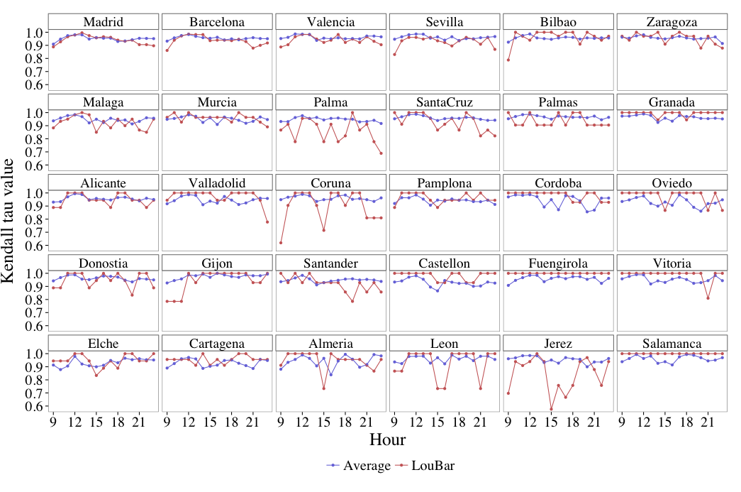
The permanent hotspots are the most important locations in the city in terms of individuals density. An interesting question is whether their rank (according to the density) is constant or changes during the day. In order to test the stability in time of the hierarchy of permanent hotspots, we compute the Kendall tau value $\tau(t)$ of the set of permanent hotspots (see the Methods section for definition and for the plots). Our results show that the heart of the cities is indeed very stable both in space and in time, whatever their size.

Spatial structure of the hotspots

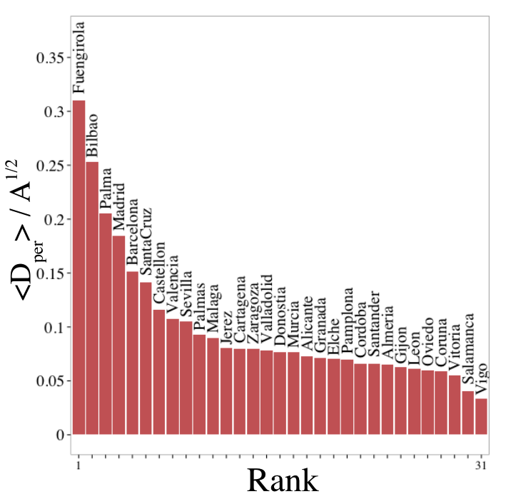
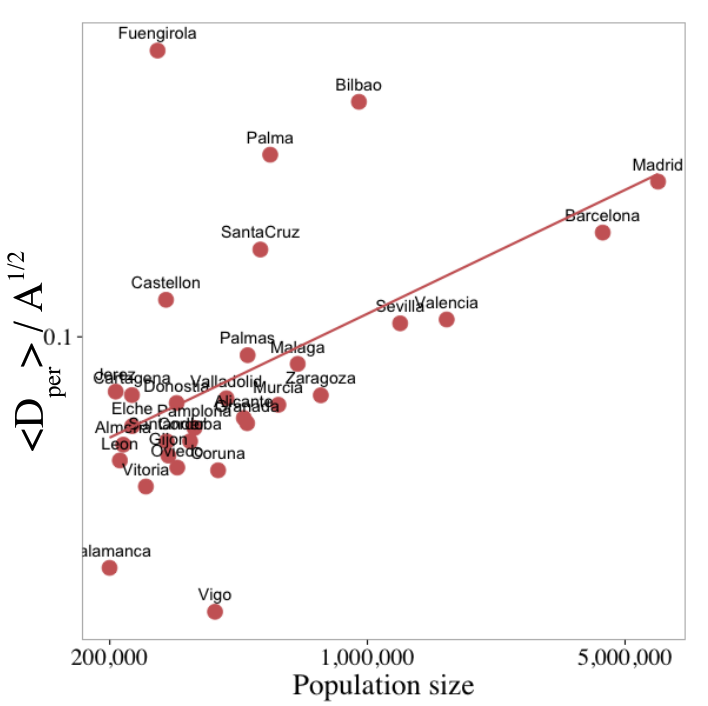
Another important question about hotspots concerns their spatial organization. We start with the specific group formed by the permanent hotspots, as defined by our more restrictive criteria ‘LouBar’ (see Methods section). We compute how distant they are from each other, compared to the typical size of the city given by $\sqrt{A}$, where $A$ is the city’s area. We show in Figure 9 the rank-plot of our ‘compacity coefficient’ defined as

$$C(i)=\frac{\langle D_{per(i)}\rangle}{\sqrt{A_{i}}}$$ (3)

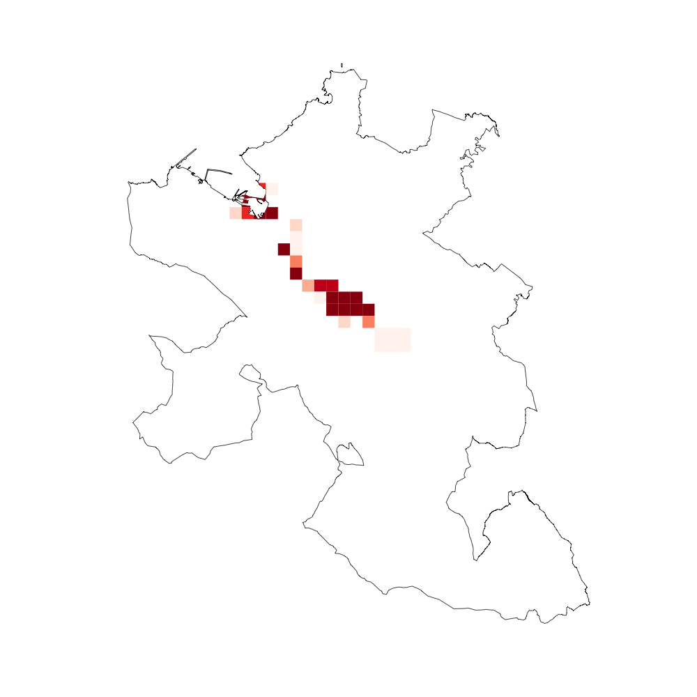
where $\langle D_{per(i)}\rangle$ is the average distance between permanent, weekday hotspots in city $i$, and $A_{i}$ is the area of the city $i$. This indicator informs us how the permanent hotspots are sprawled all over the city’s space, and it is thus a measure of the compacity of the city core: for cities with values around 0, the permanent hotspots are very close to one another, when compared to the spatial extension of the urban area. On the contrary, a value close to one indicates that these always-crowded places are spread all over the whole city space (see figure 9).

(a)	(b)
(c)	(d)

Figure 9: Different spatial structure of hotspots in cities. Rank plot of the compacity coefficient $C=\langle D_{per}\rangle/\sqrt{A}$ among the 31 metropolitan areas. (b) Compacity versus population size. We observe a trend (at least for a large subset of cities, the corresponding fit is shown as a guide to the eye). (c) and (d) The spatial organization of the $1km2$ permanent hotspots determined by the Loubar method, in the urban areas of Bilbao ($950,000$ inhabitants) and Vitoria ($250,000$ inhabitants). These figures reveal two types of spatial organization: polycentric in the case of Bilbao (c), whose permanent hotspots are not contiguous and more spread over the space of the urban area, and clearly compact and monocentric in the case of Vitoria (d).

It is interesting to note in Figure 9(b) that the compacity of a city seems to increase with the population size. At least for a large subset of cities, we indeed observe this trend, which is consistent with the idea that the larger the city, the more spread are the hotspots (and the more polycentric it tends to be).

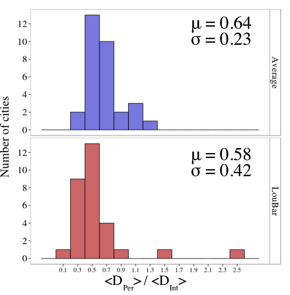
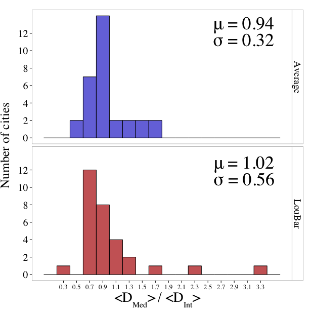
For each city, once we have determined the hotspots and have classified them into permanent, intermediary and intermittent, we measure the average distance between hotspots within each group. For example we can look at $\langle D_{int~{}hotspots}\rangle/\langle D_{per~{}hotspots}\rangle$, the ratio between the typical distance separating intermittent hotspots and the typical distance separating permanent hotspots. Since the intermittent hotspots are those with a lifespan of six hours at most, they are more inclined to capture the residential locations, while the permanent hotspots represent the dominant places of the city, that is, zones that are very dense both during daytime and nightime. On Figure 10 (a) we plot the histogram of this ratio for all cities, for the two hotspots delimitation criteria (see section Methods for these plots with different sizes of the aggregation grid). We can see in this plot that the distribution is centered around 0.6 (with similar results for the more restrictive Loubar criterion). We also computed the ratio of the average distance between intermittent hotspots and the average distance between intermediary hotspots (i.e. those that are not intermittent or permanent, so those who are present between 7 and 23 hours per day). We plot the histogram of this ratio for all 31 cities in Figure 10 (b). The distribution is peaked around 0.95-1, with lower values of standard deviation, which means that intermittent and intermediate hotspots are, on average, as much dispersed and that the significative differences lie in the spatial organization of permanent hotspots vs. non permanent hotspots.

(a)	(b)

Figure 10: Histograms of the coefficients $<D_{per}>/<D_{int}>$ (a) and $<D_{med}>/<D_{int}>$ (b). While the spatial features of intermittent and intermediary hotspots are similar, the main difference between cities lies in how the permanent hotspots are distributed in space.

Discussion

We have shown in this study that it is possible to extract relevant information from mobile phone data, not only about the mobility behavior of individuals, but also about the structure of the city itself. We have defined various indices that allow us to propose a new classification of cities based on their dynamical properties. We have also presented a method to determine the dominant centers, the hotspots, and we have confirmed recent results -obtained on completely different data- showing that the number of activity centers in cities scales sublinearly with the population size of the city. We have also highlighted some properties of hotspots such as the strong stability of the hierarchy of city centers along the day, whatever the city size. These results constitute a step towards a quantitative typology of cities and their spatial structure, an important ingredient in the construction of a science of cities.

Methods

Spatial delimitation of cities

Comparing the spatial structure of cities of very different population sizes and areas requires to rely on a harmonized definition of cities that goes beyond the arbitrariness of the spatial boundaries of the administrative units bretagnolle_time_2002 ; bretagnolle_organisation_2009 . To that extent, we have chosen to rely on the urban areas defined by the AUDES initiative (Areas Urbanas De ESpaña) which capture some coherent delimitations of cities regarding the home-work commuting patterns of individuals living in the core city of the metropolitan areas and in their surrounding municipalities. These delimitations are built upon statistical criteria based on the proportion of residents of surrounding municipalities that commute to the main city to work.

Average distance between individuals and dilatation index

We started with the Venables index pereira_urban_2013 , defined as:

$$V=\sum_{i\neq j}s_{i}s_{j}d_{i,j}$$ (4)

with $s_{i}(t)=n_{i}(t)/N(t)$ the share of individuals present in cell $i$ at time $t$, and $d_{ij}$ the distance between $i$ and $j$. When all activity is concentrated in one spatial unit only, the minimum value zero of $V$ is reached. An important point of this dilatation index is that one doesn’t need to determine hotspots to compute it. By normalizing $V$ by the densities, we can compute a weighted average distance, the ‘Venables distance’

$$D_{V}(t)=\frac{\sum_{i<j}s_{i}(t)s_{j}(t)d_{ij}}{\sum_{i<j}s_{i}(t)s_{j}(t)}$$ (5)

with $s_{i}(t)=n_{i}(t)/N(t)$ the share of individuals present in cell $i$ at time $t$. In order to compare the value of $D_{V}$ across cities, we compute $D_{V}(t)/\sqrt{A}$ with $A$ the area of the city. By considering all pairs of cells and weighting their distance by the densities of individuals in each of them, $D_{V}(t)$ signals how much the important places of the city at time $t$ are distant from each other.

Identification of the hotspots

The data gives access to the spatial density $\rho(i,t)$ of users at different moments. The full density is a complex object and we have to extract relevant and useful information. The locations that display a density much larger than the others - the hotspots - give a good picture of the city by showing where most of the people are. The hotspots thus contain important information about points of interest and activities in the city.

The determination of centres and subcentres is a problem which has been broadly tackled in urban economics giuliano1991subcenters ; mcmillen2001nonparametric ; mcmillen2003number . Starting from a spatial distribution of densities, we have to identify the local maxima. This is in principle a simple problem solved by the choice of a threshold $\delta$ for the density $\rho$: a cell $i$ is a hotspot at time $t$ if the instantaneous density of users $\rho(i,t)>\delta$. This is for example what was done in giuliano1991subcenters to determine employment centres in Los Angeles. It is however clear that this method introduces some arbitrariness due to the choice of $\delta$, and also requires prior knowledge of the city to which it is applied to choose a relevant value of $\delta$. Nonparametric methods have also been applied to determine the number of centres, some based on the regression of the natural logarithm of employment density on distance from the centre mcmillen2001nonparametric , some on the exponent of the negative exponential fit of the density distribution griffith1981modelling . Limits of these methods stand in the fact that they return a unique number of centres that could be biased when the actual density distribution is not properly fitted by an exponential law. Here we will propose an alternative method that allows us to control the impact of this choice.

A first simple criterion is to choose the point that corresponds to the average $m(t)=\overline{\rho(i,t)}$ of the distribution at time $t$ : all the cells whose density is larger than $m$ are hotspots. This is indeed a weak definition of what can be considered as a hotspot, and we propose here to use it as a ‘lower’ bound $\delta_{min}=m$.

In order to understand how the various properties of hotspots will depend on this definition, we introduce a more restrictive definition which will be considered as an upper bound of what can be considered as a hotspot. In the following we discuss how to find this upper bound. In order to characterize the disparity of the activity in the city and to isolate the dominant places, we first plot the Lorenz curve of the density distribution in the city at each hour. The Lorenz curve, a standard object in economics, is a graphical representation of the cumulative distribution function of an empirical probability distribution. For a given hour, we have the distribution of densities $\rho(i,t)$ and we sort them in increasing rank, and denote them by $\rho(1,t)<\rho(2,t)<...<\rho(n,t)$ where $n$ is the number of cells. The Lorenz curve is constructed by plotting on the x-axis the proportion of cells $F=i/n$ and on the y-axis the corresponding proportion of users density $L$ with:

$$L(i,t)=\frac{\sum_{j=1}^{i}\rho(j,t)}{\sum_{j=1}^{n}\rho(j,t)}$$ (6)

If all the densities were of the same order the Lorenz curve would be the diagonal from $(0,0)$ to $(1,1)$. In general we observe a concave curve with a more or less strong curvature, and the area between the diagonal and the actual curve is related to the Gini coefficient, an important indicator of inequality used in economics.

In the Lorenz curve, the stronger the curvature the stronger the inequality and, intuitively, the smaller the number of hotspots. This remark allows us to construct a new criterion by relating the number of dominant hotspots (i.e. those that have a very high value compared to the other cells) to the slope of the Lorenz curve at point $F=1$: the larger the slope, the smaller the number of dominant individuals in the statistical distribution. The natural way to identify the typical scale of the number of hotspots is to take the intersection point $F^{*}$ between the tangent of $L(F)$ at point $F=1$ and the horizontal axis $L=0$ (see Figure 11). This method is inspired from the classical scale determination for an exponential decay: if the decay from $F=1$ were an exponential of the form $\exp{-(1-F)/a}$ where $a$ is the typical scale we want to extract, this method would give $1-F^{*}=a$.

Figure 11: Illustration of the criteria selection on the Lorenz curve.

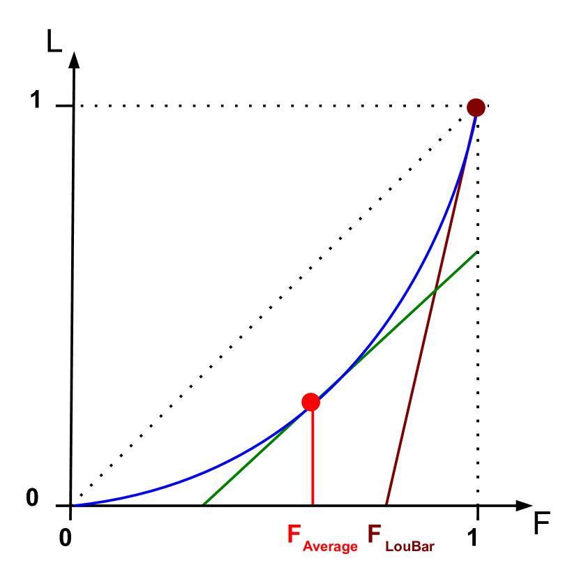
We note here that the average criterion corresponds to the point of the Lorenz curve with slope equal to $1$. Indeed, the general expression of the Lorenz curve for the set of densities $\rho(i,t)$ whose cumulative function is $F(\rho)$ is:

$$L(F)=\frac{1}{m}\int_{0}^{F}\rho(F)dF$$ (7)

where $\rho(F)$ is the inverse function of the cumulative. This point thus satisfies

$$\frac{dL}{dF}=1$$ (8)

which gives $m=\rho(F_{Avg})$ or in other words, the hotspots will be those with densities larger than the average. In contrast, our more restrictive criterion based on the slope at $F=1$ gives

$$F^{*}=1-\frac{\mu}{\rho_{M}}$$ (9)

where $\rho_{M}$ is the maximum value of $\rho(i,t)$ (for a given time $t$). We thus see that in general $F_{Avg}<F^{*}$ and that this new criterion, more restrictive, does not only depend on the average value of the density but also on the dispersion: as $\rho_{M}$ increases, the value of $F^{*}$ increases and therefore the number of detected hotspots decreases.

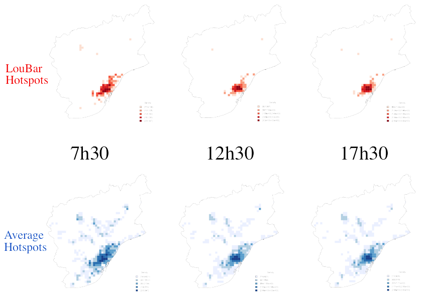
All other possible and reasonable methods will then give a value comprised in the interval $[F_{Avg},F^{*}]$ between the average criterion and our criterion (also denoted by ‘LouBar’). Instead of choosing a particular point, we will thus study most of the properties computed for hotspots with the two methods, giving us both a lower and upper bounds. In particular, we will be able to test the robustness of our results against the arbitrariness of the hotspot identification method. Figure 12 shows the location of the hotspots selected according to the two methods/criteria at different moments of the day, in the metropolitan area of Barcelona. These maps can be regarded as the extremes of hotspots maps that reasonable delimitation methods could produce (i.e. with a number of hotspots comprised between $F_{Avg}$ and $F^{*}$.

Figure 12: Location of the hotspots in the metropolitan area of Barcelona, selected with two different criteria: the Average criterion and our more restrictive criterion (’LouBar’). Here density data are aggregated on a grid composed of $1km^{2}$ square cells.

Influence of the spatial scale of aggregation

Hotspots

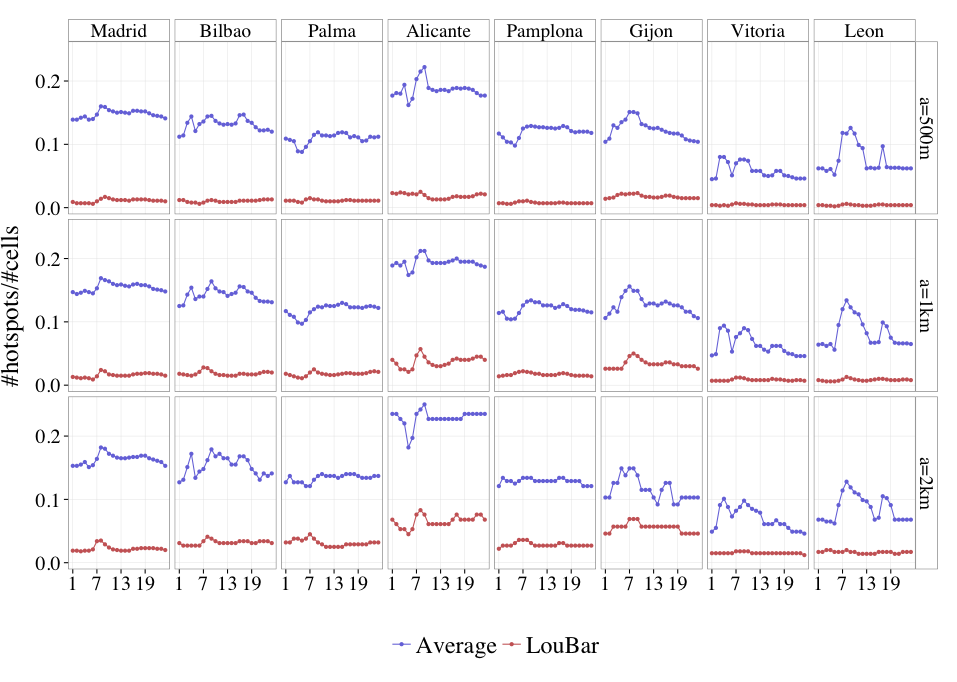
In the hotspots identification process, the size of the grid cells on which we aggregate the numbers/densities of users is another arbitrary parameter (cf. section Methods). Since we don’t want to determine this value separately for each city, we consider that several sizes should be tested for each city and that it is reasonable to consider that this cell size $a$ can vary from $500$ meters to $2$ km. Figure 13 gives an idea of how much the proportion of hotspots change from one cell size to another. The cell size $a$ should primarily be chosen based on what is considered as a reasonable size for an urban hotspot. From the pedestrian point of view, every size between 500 metres and 2 kilometres seems a priori acceptable. Below 500m, it would clearly be necessary to aggregate contiguous hotspots : for example, for $a=100m$ ($10^{-2}km^{2}$ cells), two contiguous hotspots could not as easily be distinguished as two different ones from a pedestrian point of view. In contrast, a size of $2000m$ can be considered as an upper bound for the same reasons: if two contiguous cells are classified as hotspots, it is reasonable to identify them as two distincts neighbourhoods. It is however a question of perception and should be discussed carefully. In the hypothesis of $a=1000m$ ($1km^{2}$ cells), we chose to consider that two adjacent hotspots are two different hotspots. For reasonable sizes of grid, the values of the indicators should be robust with a change of the cell size. We then tested the sensitivity of our results with respect to different resolutions.

Figure 13: Time evolution of the ratio $\frac{\#hotspots}{\#cells}$ for two hotspots definitions and different sizes of grid cells, for eight different cities of very different sizes. The cities chosen cover the full range of the poulation size distribtion of the set of the 31 cities studied. Every reasonable method for defining hotspots would give a value between the two lines of each plot. One can see that qualitatively pattern stays identical whatever the grid size for couple (city, method).

Number of hotspots

In Figure 14 we show the scaling relation between the number of hotspots with the population and the effect of the grid size. Here we see that the scaling results and the value of the exponent are robust against a change in (i) the threshold used for identifying the hotspots and (ii) the size of the grid cells.

Figure 14: Scatter plot and model fit line of the number of hotspots $H$ vs. the population size $P$ for the 31 cities studied. Each point in the scatterplot corresponds to the average number of hotspots determined for each one-hour time bin of a weekday time period considered for the five weekdays. The linear relationship on a log-log plot indicates a power-law relationship between the two quantities, with an exponent value $\beta<1$, indicating that the number of activity centers in a city grows sublinearly with its population size.

Kendall’s $\tau$

Definition

The Kendall rank coefficient is used as a test statistic to establish whether two lists of random variables may be regarded as statistically dependent. To each cell $i$ we associate its rank $r_{i}(t)$ in the ordered density distribution at time $t$. Kendall’s $\tau$ value indicates how much the hierarchy changed between $t-1$ and $t$. For a set of pairs $(i,j)$, it is equal to the difference between the number of converging pairs (i.e. $\rho_{i}$ was larger (resp. smaller) than $\rho_{j}$ at $(t-1)$ and is still larger (resp. smaller) at $t$) and the number of diverging pairs ($\rho_{i}$ was smaller (resp. larger) than $\rho_{j}$ at $(t-1)$ and is larger (resp. smaller) at $t$). The Kendall values $\tau(t)$ are plotted on Figure 15.

Under the null hypothesis of independence of two lists, the distribution of $\tau$ has an expected value of zero and for larger samples, the variance is given by

$$\overline{\tau^{2}}=\frac{2(2n+5)}{9n(n-1)}$$ (10)

Any value of $\tau$ larger than this null-value signals the existence of relevant correlations.

Hierarchy stability

We show in Figure 15 the evolution of Kendall $\tau$ values calculated for the set of permament hotspots during daytime in an average weekday, for 31 Spanish urban areas with more than 200,000 inhabitants. The curves are ranged by decreasing order of population size (the biggest city in the top left corner, the smallest in the bottom right). The red curves correspond to the daytime evolution of the Kendall $\tau$ for the hotspots selected with the ‘LouBar’ more restrictive criterion, the blue ones to the Kendall $\tau$ of the hotspots selected with the ’Average’ criterion. These results indicate that the hierarchy of permanent hotspots is indeed very stable in time.

Figure 15: Evolution of Kendall $\tau$ values for permament hotspots during daytime for an average weekday.

Author Contributions

T.L. designed the study, analysed the data and wrote the manuscript; M.L. processed and analysed the data; O.G.C and M.P. processed the data; R.H. and J.J.R. coordinated the study; E.F.-M. obtained and processed the data; M.B. coordinated and designed the study, and wrote the manuscript. All authors read, commented and approved the final version of the manuscript.

References

- (1) Asgari F, Gauthier V, Becker M (2013) A survey on human mobility and its applications. arXiv:13070814 [physics].
- (2) Gallotti R, Bazzani A, Rambaldi S (2012) Towards a statistical physics of human mobility. International Journal of Modern Physics 23.
- (3) Furletti B, Cintia P, Renso C, Spinsanti L (2013) Inferring human activities from gps tracks. In: UrbComp 2013 Chicaco, USA, August 11.
- (4) Roth C, Kang SM, Batty M, Barthélemy M (2011) Structure of urban movements: polycentric activity and entangled hierarchical flows. PloS one 6: e15923.
- (5) Hawelka B, Sitko I, Beinat E, Sobolevsky S, Kazakopoulos P, et al. (2013) Geo-located twitter as the proxy for global mobility patterns. arXiv:13110680 [physics].
- (6) Noulas A, Scellato S, Lambiotte R, Pontil M, Mascolo C (2012) A tale of many cities: Universal patterns in human urban mobility. PLoS ONE 7: e37027.
- (7) Onnela JP, Saramäki J, Hyvönen J, Szabó G, Lazer D, et al. (2007) Structure and tie strengths in mobile communication networks. Proceedings of the National Academy of Sciences 104: 7332.
- (8) Lambiotte R, Blondel VD, de Kerchove C, Huens E, Prieur C, et al. (2008) Geographical dispersal of mobile communication networks. Physica A: Statistical Mechanics and its Applications 387: 5317–5325.
- (9) Gonzalez MC, Hidalgo CA, Barabasi AL (2008) Understanding individual human mobility patterns. Nature 453: 779–782.
- (10) Schneider CM, Belik V, Couronné T, Smoreda Z, González MC (2013) Unravelling daily human mobility motifs. Journal of The Royal Society Interface 10.
- (11) Kung KS, Sobolevsky S, Ratti C (2013) Exploring universal patterns in human home/work commuting from mobile phone data. arXiv:13112911[physics].
- (12) Pei T, Sobolevsky S, Ratti C, Shaw SL, Zhou C (2013) A new insight into land use classification based on aggregated mobile phone data. arXiv:13106129 [cs].
- (13) Sobolevsky S, Szell M, Campari R, Couronné T, Smoreda Z, et al. (2013) Delineating geographical regions with networks of human interactions in an extensive set of countries. arXiv:13101829 [physics].
- (14) Anas A, Arnott R, Small KA (1997) Urban spatial structure. University of California - Transportation Center.
- (15) Bertaud A, Malpezzi S (2003) The spatial distribution of population in 48 world cities: Implications for economies in transition. Report, World Bank.
- (16) Tsai YH (2005) Quantifying urban form: compactness versus sprawl. Urban Studies 42: 141–161.
- (17) Pereira RHM, Nadalin V, Monasterio L, Albuquerque PHM (2013) Urban centrality: A simple index. Geographical Analysis 45: 77–89.
- (18) Schwarz N (2010) Urban form revisited - selecting indicators for characterising european cities. Landscape and Urban Planning 96: 29–47.
- (19) Thomas I, Frankhauser P, Biernacki C (2008) The morphology of built-up landscapes in wallonia (belgium): A classification using fractal indices. Landscape and Urban Planning 84: 99–115.
- (20) Guérois M, Pumain D (2008) Built-up encroachment and the urban field: a comparison of forty european cities. Environment and Planning A 40: 2186–2203.
- (21) Berroir S, Mathian H, Saint-Julien T, Sanders L (2011) The role of mobility in the building of metropolitan polycentrism. In: Desrosiers F, Thériault M, editors, Modelling urban dynamics, ISTE-Wiley. pp. 1–25.
- (22) Le Néchet F (2012) Urban spatial structure, daily mobility and energy consumption: a study of 34 european cities. Cybergeo : European Journal of Geography.
- (23) Openshaw S, Taylor PJ (1979) A million or so correlation coefficients: three experiments on the modifiable areal unit problem. Statistical applications in the spatial sciences 21: 127–144.
- (24) Louf R, Barthelemy M (2013) Modeling the polycentric transition of cities. Physical Review Letters 111.
- (25) Arcaute E, Hatna E, Ferguson P, Youn H, Johansson A, et al. (2013) City boundaries and the universality of scaling laws. arXiv:13011674 [physics].
- (26) Bretagnolle A, Pumain D, Vacchiani-Marcuzzo C (2009) The organisation of urban systems. Complexity perspective in innovation and social change : 197–220.
- (27) Bretagnolle A, Paulus F, Pumain D (2002) Time and space scales for measuring urban growth. Cybergeo : European Journal of Geography.
- (28) Giuliano G, Small KA (1991) Subcenters in the los angeles region. Regional science and urban economics 21: 163–182.
- (29) McMillen DP (2001) Nonparametric employment subcenter identification. Journal of Urban Economics 50: 448–473.
- (30) McMillen DP, Smith SC (2003) The number of subcenters in large urban areas. Journal of Urban Economics 53: 321–338.
- (31) Griffith DA (1981) Modelling urban population density in a multi-centered city. Journal of Urban Economics 9: 298–310.