Kosterlitz-Thouless and Potts transitions in a generalized XY model

Abstract

We present extensive numerical simulations of a generalized XY model with nematic-like terms recently proposed by Poderoso et al [PRL 106(2011)067202]. Using finite size scaling and focusing on the $q=3$ case, we locate the transitions between the paramagnetic (P), the nematic-like (N) and the ferromagnetic (F) phases. The results are compared with the recently derived lower bounds for the P-N and P-F transitions. While the P-N transition is found to be very close to the lower bound, the P-F transition occurs significantly above the bound. Finally, the transition between the nematic-like and the ferromagnetic phases is found to belong to the 3-states Potts universality class.

I Introduction

Two dimensional systems with short-range interactions can not break continuous symmetry. This is the reason why neither true crystals, ferromagnets, or nematics can exist in 2D Mermin and Wagner (1966). Nevertheless, at low temperatures these systems can exhibit a quasi-long range order, with the correlation functions decaying with distance as a power law. The transition between the “ordered” and disordered phases is often found to be of infinite order and to belong to the Kosterlitz-Thouless (KT) universality class Kosterlitz and Thouless (1973); Kosterlitz (1974). The transition is driven by the unbinding of topological charges (vortices). At low temperature the charges are bound in dipolar vortex-antivortex pairs, while at high temperature the vortices unbind and lead to the destruction of the quasi long-range order. Unlike the usual thermodynamic phases, the low temperature KT phase is critical for all temperatures and is characterized by a discontinuous jump of the helicity modulus, which is the order parameter that measures how the system responds to a global twist Fisher et al. (1973); Nelson and Kosterlitz (1977); Ohta and Jasnow (1979).

A generalization of the XY model, including nematic-like terms, has been recently introduced and studied by several authors for both $q=2$ Korshunov (1985); Lee and Grinstein (1985); Lee et al. (1986); van Himbergen (1986); Sluckin and Ziman (1988); Carpenter and Chalker (1989); Zukovic et al. (2001); Messager and Nachtergaele (2006); Park et al. (2008); Komendová and Hlubina (2010); Dian and Hlubina (2011); Shi et al. (2011); Hübscher and Wessel (2013) and integers $q>2$ Romano (2006); Poderoso et al. (2011),

$${\cal H}=-\sum_{\langle ij\rangle}[\Delta\cos(\theta_{i}-\theta_{j})+(1-\Delta)\cos(q\theta_{i}-q\theta_{j})],$$ (1)

with $0\leq\Delta\leq 1$, $0\leq\theta_{i}\leq 2\pi$ and nearest neighbors interactions. Similar models have recently been considered in the contexts of collective motion of active nematics Ngo et al. (2012) and Hamiltonian mean field models Teles et al. (2012). For $\Delta=1$, one recovers the usual XY model with the critical temperature $T_{\scriptstyle\rm KT}(1)\simeq 0.893$. Changing variables in the partition function, $q\theta_{i}\rightarrow\bar{\theta}_{i}$, shows that the $\Delta=0$ model is also isomorphic to the XY model with the same critical temperature (see also Ref. Carmesin (1987)), $T_{\scriptstyle\rm KT}(0)=T_{\scriptstyle\rm KT}(1)$. In between, when $0<\Delta<1$, Eq.(1) describes the competition between directional and nematic-like alignment (i.e., $2k\pi/q$ with integer $k\leq q$), with a line of critical points $T_{\scriptstyle\rm KT}(\Delta)$. In general, besides the high temperature, paramagnetic (P) phase, there are at least two other phases that are extensions of the phases occurring at $\Delta=0$ and $\Delta=1$. A quasi long-range ferromagnetic (F) phase exists for all values of $\Delta$ and extends down to zero temperature (because parallel spins minimize both terms of the Hamiltonian, while nematic-like ordering minimizes only the second term). For small values of $\Delta$, there is an intermediate temperature phase with nematic-like (N) quasi long-range order. A second order phase transition line is found to separate F and N phases, ending in a multicritical point at $\Delta_{\scriptstyle\rm mult}$. Only recently the phase diagram for $q=2$ has been precisely obtained Hübscher and Wessel (2013). In a recent paper, Poderoso et al have studied Poderoso et al. (2011) the $q$-nematic N to F transition for the $q=3$ model. This transition was found to belong to the 3-states Potts universality class. The P-N and P-F transitions were expected to belong to the KT class, however, neither the location nor the universality class of these transitions was precisely determined in Ref. Poderoso et al. (2011). Using heuristic arguments Korshunov Korshunov (2012), suggested that for $q>2$ a $q$-nematic phase is impossible . This, however, clearly contradicted the results of the simulations of Poderoso et al Poderoso et al. (2011). Furthermore, the mapping between $\Delta=0$ and 1 shows that the N phase exists at least for $\Delta=0$. Using Ginibre’s inequality Ginibre (1970) it can then be shown Romano (2006) that the N-P transition must also extend to finite $\Delta$. Ginibre’s inequality also provides a rigorous lower bound Romano (2006) for the transition temperature between P and N phases, $T_{\scriptstyle\rm KT}(\Delta)\geq(1-\Delta)T_{\scriptstyle\rm KT}(0)$ for $\Delta<\Delta_{\scriptstyle\rm mult}$. For $\Delta>\Delta_{\scriptstyle\rm mult}$, the KT transition is between P and F phases Romano (2006), with the lower bound given by $T_{\scriptstyle\rm KT}(\Delta)\geq T_{\scriptstyle\rm KT}(0)\Delta$. Since at very low temperature the system must be in the F phase, this proves the existence of all three phases for small, but finite $\Delta$. The objective of the present work is to precisely calculate the phase diagram for the $q=3$ generalized XY model and to compare the critical temperatures for the P-N and P-F transitions with the bounds obtained in Ref. Romano (2006). Moreover, since the very existence of the N-P transition has been contested for $q>2$ Korshunov (2012), it is important to present a broad set of solid evidences supporting such a transition.

II Simulations

The simulations were performed on a square lattice of linear size $L$ and periodic boundary conditions. Both Metropolis single-flip and Wolff cluster algorithms Wolff (1989) were used. The phase transitions are characterized by observables such as the generalized magnetizations and the corresponding susceptibilities,

$$m_{k} =\frac{1}{L^{2}}\left|\sum_{i}\exp(ik\theta_{i})\right|$$ (2)

$$\chi_{k} =\beta L^{2}(\langle m_{k}^{2}\rangle-\langle m_{k}\rangle^{2})$$ (3)

where $k=1,\ldots,q$, and the Binder cumulants Loison (1999); Hasenbusch (2008),

$$U_{k}=\frac{\langle m_{k}^{2}\rangle^{2}}{\langle m_{k}^{4}\rangle}.$$ (4)

Since there is no long-range order in 2d, the observables $m_{k}$ are not, strictly speaking, the order parameters for the phase transition. The order parameter for KT transition is the helicity modulus $\Upsilon$ which, in the thermodynamic limit, is zero in the disordered phase and remains finite in the ordered phase. It is defined as the response upon a small, global twist along one particular direction. Following Ref. Minnhagen and Kim (2003), it can be written as $\Upsilon=e-L^{2}\beta s^{2}$, where $e\equiv L^{-2}\sum_{\langle ij\rangle_{x}}U_{ij}^{\prime\prime}(\phi)$ and $s\equiv L^{-2}\sum_{\langle ij\rangle_{x}}U_{ij}^{\prime}(\phi)$ (the sum is over the nearest neighbors along the horizontal direction), $\phi=\theta_{i}-\theta_{j}$ and $U_{ij}(\phi)$ is the potential between spins $i$ and $j$. For the Hamiltonian Eq. (1) Hübscher and Wessel (2013),

$$\Upsilon =\frac{1}{L^{2}}\sum_{\langle ij\rangle_{x}}\left[\Delta\cos\phi+q^{2}(1-\Delta)\cos(q\phi)\right]$$

$$-\frac{\beta}{L^{2}}\left(\sum_{\langle ij\rangle_{x}}\left[\Delta\sin\phi+q(1-\Delta)\sin(q\phi)\right]\right)^{2}.$$ (5)

For the XY model with $\Delta=1$, the critical temperature is determined by the condition $\Upsilon(T_{\scriptstyle\rm KT})=2T_{\scriptstyle\rm KT}/\pi$ Fisher et al. (1973); Nelson and Kosterlitz (1977). The isomorphism between the ferromagnetic XY model with $\Delta=1$ and a purely $q$-nematic model with $\Delta=0$ requires that the critical temperature must be the same for both models. The helicity modulus for the $q$-nematic, however, contains an extra factor of $q^{2}$ which must be accounted for in the condition for criticality. Following Ref. Hübscher and Wessel (2013) the location of the KT transition will be determined by the asymptotic crossing point of $\Upsilon$ and the line $2T_{\scriptstyle\rm KT}/\lambda^{2}\pi$. The factor $\lambda$ is related to the charge of the topological excitation. For the F-P transition ($q=1$), $\lambda=1$ and the transition is driven by the unbinding of integer vortices. For $q=2$, $\lambda=1/2$ in the N phase, corresponding to half-integer vortices (connected by domain walls). In general, $\lambda=1/q$ for the $q$-nematic-paramagnetic transition.

For the N-F transition the usual finite size scaling (FSS) analysis provides the critical exponents $\beta,\gamma,$ and $\nu$: $m=L^{-\beta/\nu}f(tL^{1/\nu})$ and $\chi=L^{\gamma/\nu}g(tL^{1/\nu})$, where $m$ is the order parameter and $\chi$ is its susceptibility, $f$ and $g$ are the scaling functions, and $t=T/T_{c}-1$ is the reduced temperature. Indeed, for $q=3$ this transition is in the universality class of the 3-states Potts model with $\nu=5/6$, $\beta=1/9$ and $\gamma=13/9$, and has been studied in detail in Ref. Poderoso et al. (2011). However, the KT transition has an essential singularity, the correlation length grows exponentially, and this FSS is no longer valid. Furthermore, the whole low temperature phase is critical and both the correlation length and the susceptibility are infinite in the thermodynamic limit Kosterlitz (1974); Tobochnik and Chester (1979). Nevertheless, for all temperatures $T\leq T_{\scriptstyle\rm KT}$, the critical exponent ratios are well defined and the magnetization and the associated susceptibility scale, respectively, as $m\propto L^{-\beta/\nu}$ and $\chi\propto L^{\gamma/\nu}$. Exactly at the transition, $\beta/\nu=1/8$ and $\gamma/\nu=7/4$, which are the same ratios as for the 2d Ising model. Below the phase transition temperature the critical exponents are non-universal.

Figure 1: (Top) Average magnetization $m_{1}$ and $m_{3}$ Poderoso et al. (2011) for $\Delta=0.25$ and several system sizes $L$ showing the N-F phase transitions at $T_{\rm Potts}\simeq 0.36$ and P-N transition at $T_{\scriptstyle\rm KT}\simeq 0.67$. (Bottom) Average helicity modulus $\Upsilon$ versus $T$. The crossing of the helicity with the line $18T/\pi$ (see text for an explanation) at $T_{\scriptstyle\rm KT}(L)$ gives, for $L\to\infty$, $T_{\scriptstyle\rm KT}\simeq 0.67$. Notice also that the system sizes used here are considerably larger than those in Ref. Poderoso et al. (2011).

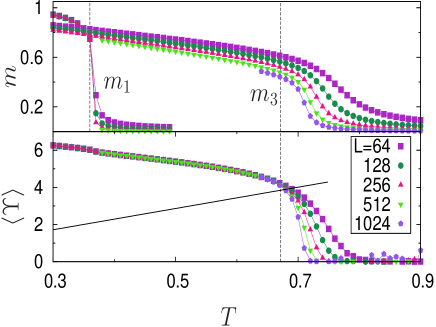
Results for the average magnetizations $m_{1}$ and $m_{3}$ are shown in Fig. 1 (top) for $\Delta=1/4$. For this $\Delta$ the critical temperature for the N-F transition was found to be $T_{\rm Potts}(0.25)\simeq 0.365$ Poderoso et al. (2011) at which $m_{1}$ drops to very low values. On the other hand, the nematic magnetization $m_{3}$ clearly shows the N-P transition. At the transition temperature $T_{\scriptstyle\rm KT}$, $m_{3}$ behaves as $m_{3}(T_{\scriptstyle\rm KT})\sim L^{-0.128}$ (not shown). The exponent is very close to the KT value, $\beta/\nu=1/8$. In the bottom part of Fig. 1, the averaged data for the helicity modulus $\Upsilon$ Fisher et al. (1973) for $\Delta=0.25$ is shown along with the line $18T/\pi$. Following Refs. Weber and Minnhagen (1988); Hübscher and Wessel (2013), we first fit the helicity modulus data for a fixed temperature assuming a logarithmic approach to its asymptotic value:

$$\Upsilon_{\scriptstyle\rm fit}(L)=\frac{2TA}{\pi}\left(1+\frac{1}{2}\frac{1}{\log L+C}\right),$$ (6)

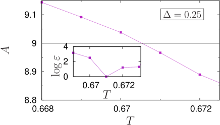
where $A$ and $C$ are fitting parameters. The constant $A$ is related to the vorticity of the system and is expected to be $A=1/\lambda^{2}$ at the transition. This form, valid at $T_{\scriptstyle\rm KT}$, was inspired by renormalization group calculations and was observed to be valid even for very small systems Weber and Minnhagen (1988). Away from $T_{\scriptstyle\rm KT}$, the above expression is no longer valid, the data deviates from it and the fitting error increases. Indeed, after repeating the process for several temperatures close to the transition, the critical temperature corresponds to the one that minimizes the normalized quadratic error,

$$\varepsilon=\sum_{i}\left(\frac{\langle\Upsilon(T,L_{i})\rangle-\Upsilon_{\scriptstyle\rm fit}(T,L_{i})}{\sigma(T,L_{i})}\right)^{2},$$ (7)

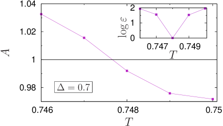
with $\sigma(T,L_{i})=\sqrt{\langle\Upsilon^{2}\rangle-\langle\Upsilon\rangle^{2}}$. Following this procedure we obtain, for $\Delta=0.25$, $T_{\scriptstyle\rm KT}\simeq 0.671$ and $A\simeq 8.97$ ($\lambda\simeq 1/3$). Within error bars, this value is the same as the lower bound. For the F-P transition one expects $\lambda=1$ and, repeating the same procedure one gets, for $\Delta=0.7$, $A\simeq 0.99$ and $T_{\scriptstyle\rm KT}\simeq 0.748$.

Figure 2: The susceptibility $\chi_{3}(T)$ associated with $m_{3}$ near the KT transition for $\Delta=0.25$. Notice that $\chi_{3}$ grows with the system size even far below the critical temperature. At the transition, the peak increases as $\chi_{3}(T_{\scriptstyle\rm KT})\sim L^{1.755}$, where the exponent was obtained from the fit shown in the inset.

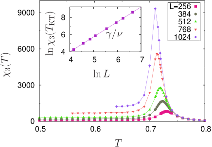
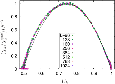
Fig. 2 shows that the susceptibility $\chi_{3}$ diverges for all temperatures below $T_{\scriptstyle\rm KT}$ as $L\rightarrow\infty$. The exponent is clearly non universal and is larger in the critical region. For a KT phase transition, for increasing $L$, one expects $\chi_{3}(T_{\scriptstyle\rm KT})\sim L^{\gamma/\nu}$, with $\gamma/\nu=7/4$. Indeed, we find $\chi_{3}(T_{\scriptstyle\rm KT})\sim L^{1.755}$, as can be seen in the inset of Fig. 2. Further evidence of the transition can be obtained from the Binder cumulant, Eq. (4), even without the knowledge of the critical temperature. Near the phase transition the Binder cumulant scales as $U=h(L/\xi)$, where $h(x)$ is a scaling function, and $\xi$ is the correlation length. On the other hand $\chi_{3}=L^{2-\eta}g(L/\xi)$, so that $\chi_{3}L^{\eta-2}=g[h^{-1}(U)]$. Therefore, by plotting $\chi_{3}L^{\eta-2}$ (with $\eta=1/4$ for KT transition) vs. the Binder cumulant Loison (1999), all the susceptibilities for different system sizes and temperatures should collapse onto one universal curve. This is precisely what is found in our simulations. Fig. 3 shows the data collapse for $U_{1}$ and $\chi_{1}$ for several values of $\Delta<0.5$ and $U_{3}$ and $\chi_{3}$ for $\Delta>0.5$. After rescaling the collapsed curves by the height of their maxima, $\chi_{k}^{\scriptscriptstyle\rm max}(\Delta)$, all points fall on the same universal curve close to the critical region (the line, a parabolic fit, is just a guide to the eyes). A probable explanation is that, despite corresponding to transitions between different phases, P-N and P-F, they are all in the KT universality class.

Figure 3: Collapse of the rescaled susceptibility vs. the Binder cumulant, $U_{k}=\langle m_{k}^{2}\rangle^{2}/\langle m_{k}^{4}\rangle$, for several values of $\Delta$. With $k=3$ we have $\Delta=0.1$ and 0.25 and, with $k=1$, $\Delta=0.6$, 0.7, 0.9 and 1. The linear size ranges from $L=96$ to 1024. The collapse is obtained with the KT value of the exponent, $\eta=1/4$. In addition, by rescaling the curves with the maximum value of each susceptibility, $\chi_{k}^{\scriptscriptstyle\rm max}(\Delta)$, the results for both P-N and P-F transitions all collapse on the same universal curve. The solid line, showing a small deviation from the parabolic behavior, is just a guide to the eyes.

Figure 4: Fit parameter $A$ of the helicity modulus for $\Delta=0.25$ (top) and 0.7 (bottom). Notice that $A$ crosses the value 9 (top), that is, $q^{2}$, and 1 (bottom) very close to the temperature in which the fitting error is minimum.

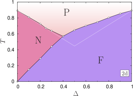
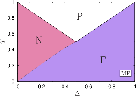
The information above can be used to construct the phase diagram for the $q=3$ generalized XY model shown in Fig. 5. Remarkably, the transition line N-P is very close to the lower bound calculated in Ref. Romano (2006) (except, close to the multicritical point). The F-P line, on the other hand, is well above the lower bound and, as a consequence, the multicritical point is located away from $\Delta=0.5$. This phase diagram is qualitatively similar to the one obtained using a simple mean-field analysis of the Hamiltonian Eq. (1). Within the mean-field approximation all the spins are connected and the Mermin-Wagner theorem does not apply. The magnetizations, $m_{1}$ and $m_{3}$, become the true order parameters, and are found to satisfy a set of coupled equations

$$m_{1} =\frac{{\cal I}_{1}(2\beta m_{1}\Delta,2\beta m_{3}(1-\Delta))}{{\cal I}_{0}(2\beta m_{1}\Delta,2\beta m_{3}(1-\Delta))}$$ (8)

$$m_{3} =\frac{{\cal I}_{3}(2\beta m_{1}\Delta,2\beta m_{3}(1-\Delta))}{{\cal I}_{0}(2\beta m_{1}\Delta,2\beta m_{3}(1-\Delta))},$$ (9)

where $\beta=1/T$, ${\cal I}_{1}(x,y)=\partial{\cal I}_{0}(x,y)/\partial x$, ${\cal I}_{3}(x,y)=\partial{\cal I}_{0}(x,y)/\partial y$ and

$${\cal I}_{0}(x,y)=\frac{1}{2\pi}\int_{0}^{2\pi}\!\!d\theta\exp\left[x\cos\theta+y\cos(3\theta)\right].$$ (10)

The free energy density is

$$f=-T\ln{\cal I}_{0}(2\beta m_{1}\Delta,2\beta m_{3}(1-\Delta))+m_{1}^{2}\Delta+(1-\Delta)m_{3}^{2}.$$ (11)

At high temperatures there is a paramagnetic phase with $m_{1}=m_{3}=0$. The phase transition between the P and F phases occurs at $T_{c}=\Delta$ for $\Delta\geq 0.5$ and the transition between the P and N phases happens at $T_{c}=1-\Delta$ for $\Delta\leq 0.5$, see Fig. 6. Both transitions are of second order. Within the N phase, $m_{1}$ is identically zero, while the nematic order vanishes as $m_{3}\sim(T_{c}-T)^{1/2}$ as the phase transition line is approached from below. On the other hand, inside the F phase the order parameters vanish as $m_{1}\sim(T_{c}-T)^{1/2}$ and $m_{3}\sim(T_{c}-T)^{3/2}$ as the F-P phase boundary is approached from below. Notice that the critical temperature for $\Delta=0$ (and 1) is $T=1$ and differ from the (smaller) KT value. As expected the fluctuations decrease the critical temperature. At lower temperatures, and $0\leq\Delta\leq 0.5$, there is a second transition at which $m_{1}$ jumps discontinuously from 0 to a finite value, corresponding to a first order transition between the N and F phases. Thus, although the nature of the phase transitions is not correctly captured by the mean field theory, both the topology of the phase diagram and the fact that the transition N-F is not in the same universality class as the transitions between P-N and P-F phases is correctly predicted.

Figure 5: Phase diagram for $q=3$. There are two KT phases, N and F, both with quasi long-range order. The points were obtained using the helicity modulus, while the lines are only guides to the eye. The transition between N and F phases is in the 3-states Potts universality class. The dashed lines are the lower bounds for the order-disorder transitions obtained in Ref. Romano (2006), $T=T_{\scriptstyle\rm KT}(0)(1-\Delta)$ and $T=T_{\scriptstyle\rm KT}(0)\Delta$ for $\Delta\leq 0.5$ and $\Delta\geq 0.5$, respectively, with a multicritical point at $\Delta_{\scriptstyle\rm mult}=1/2$ and $T_{\scriptstyle\rm KT}(1/2)=T_{\scriptstyle\rm KT}(0)/2$.

Figure 6: Mean field phase diagram for $q=3$ generalized XY model. The P-N and P-F transitions phase are continuous (solid lines) while the transition N-F (dashed line) is of first order.

III Discussion and Conclusions

In conclusion, we have studied, through extensive Monte Carlo simulations and FSS, a generalized XY model with $q=3$. Contrary to the early doubts regarding the existence of a nematic-like (N) phase in this model, as opposed to a simple crossover Korshunov (2012), we have presented strong numerical evidence that the model has P, N, and F phases. Curiously, the boundary between P and N phases coincides closely with the lower bound obtained in Ref. Romano (2006) while, on the other hand, the phase transition between F and P phases lies well above it. The transition between the N and F phases, which for $q=2$ is in the 2d Ising universality class, for $q=3$ belongs to the 3 states Potts universality class. The overall topology of the $q=2$ and 3 cases are very similar and a simple mean-field analysis is capable to grasp the existence (albeit not the actual nature) of each phase.

With the possible exception of the region around the multicritical point, the transition line N-P is very close to the lower bound (indicated in Fig. 6 by the dotted line) predicted by Romano Romano (2006). That is, the declivity of $T_{\scriptstyle\rm KT}(\Delta)$, within our precision, is $-1$. On the other hand, the line F-P has a slope smaller than unity and is located far above the lower bound. As a consequence, the multicritical point at which both lines merge is not located at $\Delta=1/2$ and is above the lower bound $T_{\scriptstyle\rm KT}/2$. These features can be observed in the phase diagram Fig. 5 and in the diagram for $q=2$ Hübscher and Wessel (2013) as well. Moreover, for different values of $q$, the multicritical point $\Delta_{\scriptstyle\rm mult}^{(q)}$ is located at increasing values of $\Delta$: $\Delta_{\scriptstyle\rm mult}^{(2)}\simeq 0.32$ Hübscher and Wessel (2013), $\Delta_{\scriptstyle\rm mult}^{(3)}\simeq 0.4$. For $q=8$, we do not yet have a precise location, but it appears to be close to $\Delta=0.5$. We observe that these points tend to the multicritical point consistent with the lower bound calculated by Romano Romano (2006), $\Delta_{\scriptstyle\rm mult}=1/2$. Thus, the F-P transition approaches, as $q$ increases, the lower bound $T_{c}(\Delta)=T_{\scriptstyle\rm KT}\Delta$ (or, possibly, there may exist a critical value of $q$ above which the lower bound might be exact).

There are several possible future extensions of this work. We are presently performing a detailed study of this model in 3d. In 2d it is important to explore the phase diagrams for larger $q$ values, since there are indications of the change in topology that occurs for larger $q$. In particular, it was observed Poderoso et al. (2011) that, differently from $q=2$ and 3, new phases appear for $q=8$. A detailed exploration of the nature of these phases is in order, not only for $q=8$ but for intermediate values as well. Finally, it has recently been proposed Shi et al. (2011); Bonnes and Wessel (2012), that for $q=2$, there may exist a region close to the multicritical point in which the transition to the paramagnetic phase is not KT, but Ising. The very existence of this Ising transition region is still an open question Hübscher and Wessel (2013) (and thus care must be taken with the use of the term multicritical). It will be interesting to see whether this topology might also extend to the larger $q$ values.