The clustering of galaxies in the SDSS-III Baryon Oscillation Spectroscopic Survey: mock galaxy catalogues for the low-redshift sample

Abstract

We present one thousand mock galaxy catalogues for the analysis of the Low Redshift Sample (LOWZ, effective redshift $z\sim 0.32$) of the Baryon Oscillation Spectroscopic Survey Data Releases 10 and 11. These mocks have been created following the PTHalos method of Manera et al. (2013) revised to include new developments. The main improvement is the introduction of a redshift dependence in the Halo Occupation Distribution in order to account for the change of the galaxy number density with redshift. These mock catalogues are used in the analyses of the LOWZ galaxy clustering by the BOSS collaboration.

1 Introduction

The Baryon Oscillation Spectroscopic Survey (BOSS, Dawson et al., 2013) is an spectroscopic survey that uses imaging data from SDSS-III (Eisenstein et al., 2011) to map over 1.35 million galaxies covering an unprecedented volume of the universe over an area of aproximately a quarter of the sky. The BOSS Data Release 11 (DR11, Anderson et al., 2013) contains $1,277,503$ galaxies covering $8498$ square degrees, which, assuming a concordance $\Lambda\textrm{CDM}$ model, results in an effective volume of $8.4$ Gpc³, the largest ever surveyed at this density.

BOSS targets two distinct galaxy samples: the CMASS sample, a high redshift sample $0.4\lesssim z\lesssim 0.7$ that selects galaxies with roughly a constant stellar mass, and a low redshift sample $0.2\lesssim z\lesssim 0.45$ that targets galaxies following an algorithm close to that designed for Luminous Red Galaxies (LRG) in SDSSS-I/II. Each of the DR11 samples has been used to fit the position of the baryon acoustic oscillation (BAO) feature, constraining the distance measurement $D_{V}$ at two per cent for LOWZ (Tojeiro et al., 2013) and one per cent in CMASS (Anderson et al., 2013). The latter is the most precise distance constraint ever obtained from a galaxy survey.

The generation of mock galaxy catalogues is an essential component to the analysis of the data from any galaxy surveys. Mocks are required for an accurate understanding of the sampling errors and the systematic errors of the clustering measurements, including the effects of cosmic variance, non-linear evolution, scale-dependend bias, redshift distortions, and discreteness effects. They also enable detailed testing of analysis pipelines. For a particular survey, mock galaxy catalogues mimic the survey geometry, the number density of objects and their selection. All key science analyses of large scale galaxy clustering from BOSS DR9 relied heavily on the mock catalogues presented in Manera et al. (2013) Science analyses of ongoing and future surveys such as the Dark Energy Survey (DES) , or in the near future HETDEX (Hill et al., 2004), DESI (Levi et al., 2013), Euclid (Laurejis et al., 2011) and LSST (Abell et al., 2009) this will also require a large suit of mock galaxy catalogues.

Ideally a set of high resolution N-body cosmological simulations, including hydrodynamics, would be run to generate the mock galaxy catalogues, but in practise the computational time that this would require is exceedingly expensive. For this reason other methods to generate a large number of galaxy mock catalogues quickly have been developed.

Manera et al. (2013), inspired by Scoccimarro and Sheth (2002), developed the PThalos method to generate fast mock galaxy catalogues. The two main steps are: i) generate a matter field using Second Order Lagrangian Perturbation Theory (2LPT) ii) populate the field with halos and galaxies, using a prescription that is calibrated against numerical simulations, and that reproduces the observed clustering of galaxies (see Section 3 for details) This method was used to create mock catalogues for the BOSS CMASS DR9 sample, which were used in analyses by Anderson et al. (2012); Tojeiro et al. (2012); Samushia et al. (2013a); Anderson et al. (2013); Reid et al. (2012); Sanchez et al. (2013).

Other methods have also been developed to generate fast galaxy mocks. Monaco et al. (2013, 2002) uses the collapsing times of dark matter particles in the Lagrangian field smoothed at several scales to fragment the dark matter field into halos, giving clustering results similar to that of PTHalos. It has also been suggested that N-body simulations could be run with low time resolution. These runs are 2-3 times slower than the methods based on a single field, but still at least within an order of magnitude or two faster than simulations. Tassev et al. (2013), suggested using 2LPT analytically at large scales, and White et al. (2013), advocate essentially to run a Particle-Mesh simulation in this way. They obtain an increasing accuracy on the mass function and clustering with respect to the perturbation theory based methods.

Finally, in order to increase the mass range of the halos from which galaxies are drawn in mocks, one can use the conditional bias of halos as a function of the local halo density (de la Torre & Peacock, 2013) use the halo mass function as a function of local mass density from a smaller size but higher resolution N-body simulations (Angulo et al., 2013), or alternatively combine the 2LPT approach for large scales with the Spherical Collapse model for small scales (Kitaura and He, 2013). We do not apply such methods here and use a mapping between the mocks and corresponding N-body simulations instead (see Section. 3 for details).

In this paper we present 1000 mock galaxy catalogues for the LOWZ DR10 and DR11 BOSS galaxy samples. These mocks were produced using the PTHalos method developed in Manera et al. (2013) but with a redshift dependence in the Halo Occupation Distribution (HOD) of galaxies in halos in order to account for the change of the galaxy number density in redshift. The mocks are fitted to the LOWZ sample clustering presented in Tojeiro et al. (2013) and the masks applied to the mocks mimic the survey geometry, observational completeness, and small-scale features such as patches of bad imaging and bright stars. These mocks have been used to provide covariance matrices and enable the study the systematic and statistical uncertainty on the BAO scale measurements presented in Anderson et al. (2013); Sanchez et al. (2013); Chuang et al. (2013). The mocks will be made publicly available.

This paper is organized as follows. In Section 2 we introduce the LOWZ sample. We summarise the PThalos method and discuss the geometry of the sample and the masks in Section 3. The HOD fitting is presented in Section 4. In Section 5 we explain the results and conclude in Section 6. Finally, tables with the covariance matrices of the LOWZ sample correlation function are provided.

2 BOSS LOWZ galaxy sample

Figure 1: DR10 (left) and DR11 (right) survey footprints in equatorial coordinates. Northern Galactic Caps on the top and Southern Galactic caps on the bottom. The color code shows the completeness of each sector.

BOSS uses SDSS CCD photometry (Gunn et al. 1998,2006) from five passbands (u, g, r, i, z; e.g., Fukugita et al. 1996) to select targets for spectroscopic observation. The LOWZ galaxy sample of BOSS targets galaxies with an algorithm that follows closely the one designed in SDSS-I/II for Luminous Red Galaxies, described in Eisenstein et al. (2001), but extending to fainter magnitudes to increase the number density. This data set has already been used by Anderson et al. (2013); Parejko et al. (2013); Tojeiro et al. (2013).

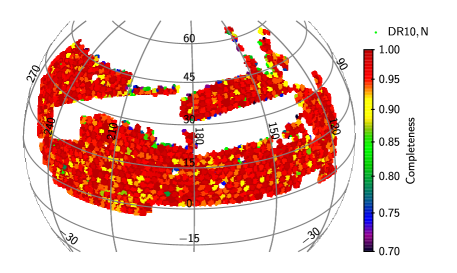
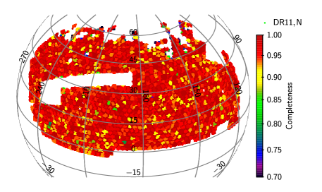
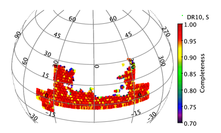
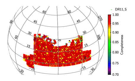
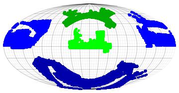
The LOWZ Data Release 10 (DR10), covers a total area of $5,635\,$deg² and is split in two separate contigous regions. One is in the Northen Galactic Cap (NGC) and covers $4,205\,$deg². The other is in the Southern Galactic Cap (SGC) and covers $1,430\,$deg². The total LOWZ DR10 sample has $218,905$ galaxies with $0.15\lesssim z\lesssim 0.43$. The DR11 covers respectively a total area of $7,998\,$deg² ($5,793\,$deg² in the NGC and $2,205\,$deg² in the SGC) and has a total of $313,780$ galaxies. The NGC footprint is smaller than that of the CMASS sample as the final target algorithm was not used for LOWZ during the first nine month of BOSS observations. The footprint of the LOWZ sample is shown in Figure 1.

Parejko et al. (2013) studied the small scale clustering of the LOWZ sample and showed that the LOWZ galaxies occupy halos of typical mass of $\sim 5\times 10^{13}$h^-1M_⊙, and galaxy bias $b\sim 2.0$. The large scale clustering of the LOWZ sample is presented in Tojeiro et al. (2013), where the observational systematics of the sample are studied in detail. The effective isotropic distance at $z=0.32$, $D_{V}=[cz(1+z)^{2}D_{A}^{2}/H]^{1/3}$, where $H$ is the Hubble parameter and $D_{A}$ the angular diameter distance, has been measured using the LOWZ BAO peak with an accuracy better than 2 per cent. The cosmological implications of this measurement when combined with the BAO measurement from the CMASS sample are presented in Anderson et al. (2013). Both papers have used the PTHalos mocks galaxy catalogues for the covariance matrices and analysis of errors.

3 Method

We have created 1000 mock galaxy catalogues for the LOWZ DR10 and DR11 galaxy samples. We use a method similar to that of Manera et al. (2013), adapted to a lower redshift and with several improvements. The mocks are such that covariance matrices can be computed and the methods of analysis of the galaxy clustering can be tested for bias and relative accuracy. The steps that we took in generating these PTHalos mocks can be summarised as follows:

3.1 Dark matter

We have run 500 dark matter particle fields based on 2LPT, using the pubicly available code 2LPTic. The matter fields were generated at redshift $z=0.32$, which is the effective pair-weighted redshift of the LOWZ sample. The matter realizations have been generated in a cubical box of size $L=2400$ h^-1 Mpc with $N=1280^{3}$ particles, for a $\Lambda$CDM cosmology with parameters $\Omega_{m}=0.274$, $\Omega_{\Lambda}=0.726$, $\Omega_{b}=0.04$, $h=0.7$, $\sigma_{8}=0.8$ and $n_{s}=0.95$, giving a particle mass $M_{p}=50.1\times 10^{10}M_{\odot}/h$ The input power spectrum has been smoothed with a cut-off as in Manera et al. (2013) as it helps the clustering of small halos. These cosmological parameters are the same as the standard fiducial choices used in BOSS analyses.

3.2 Halos

Halos have been identified in the dark matter field using a Friends-of-Friends halo-finder algorithm (FoF, Davis et al., 1985) which percolates in a halo all the particles that can be linked by within a given linking-length $l$. The value of the linking-length used in N-body simulations varies in the literature, the most common value being $l=0.2$ times the mean inter-particle distance. For a 2LPT dark matter field the value of the linking-length has to be appropriately changed in accord with the 2LPT dynamics. In the spherical collapse approximation both values can be related as follows (Manera et al., 2013):

$$l_{2LPT}=b_{N-body}\left(\frac{\Delta_{vir}^{N-body}}{\Delta_{vir}^{2LPT}}\right)^{1/3}\;,$$ (1)

where $\Delta_{vir}^{N-body}$ and $\Delta_{vir}^{2LPT}$ are the N-body and 2LPT virial overdensities. For the N-body halos we take the value of Bryan and Norman (1998) fit,

$$\Delta_{vir}^{sim}=[18\pi^{2}+82(\Omega_{m}(z)-1)-39(\Omega_{m}(z)-1)^{2}]/\Omega_{m}(z),$$ (2)

where $\Omega_{m}(z)=\Omega_{m}(1+z)^{3}H(0)/H(z)$, and $H(z)$ is the Hubble expansion value at redshift $z$. For the 2LPT halos we take $\Delta_{vir}^{2LPT}=35.4$. This value comes from the relation between the linear and non-linear density in 2LPT,

$$\Delta_{vir}^{2LPT}=\delta_{NL}^{2LPT}+1=(1-\delta_{0}D_{1}/3+\delta_{0}^{2}D_{1}^{2}/9)^{-3}\,,$$ (3)

where $\delta_{0}D_{1}=1.868$ is the value of the linear density fluctuation at collapse, and $\delta_{NL}$, its non-linear value.

Applying the above equations, we use the linking length value $l=0.388$ for halos at redshift $z=0.32$. As the value is approximate, and 2LPT lacks small scale power, the halo mass function recovered would not completely match that of an N-body simulation. Therefore, following Manera et al. (2013), we re-assigned the masses of the halos, while keeping their positions and rank-order in mass, such that we recover the Tinker et al. (2008) mass function for this cosmology. This method has been shown to match the clustering of halos in N-body simulations within 10 per cent accuracy.

3.3 Galaxies

We assign galaxies into halos by means of an Halo Occupation Distribution (HOD; Peacock & Smith 2000, Scoccimarro et al. 2001, Berlind & Weinberg 2002) functional form with five parameters, as used by Zheng et al. (2007). The mean number of galaxies in a halo of mass $M$ is the sum of the mean number of central galaxies plus the mean number of satellite galaxies, $\langle N(M)\rangle=\langle N_{cen}(M)\rangle+\langle N_{sat}(M)\rangle$, where

$$\langle N_{cen}\rangle = \frac{1}{2}\left[1+{\rm{erf}}\left(\frac{{\rm log}M-{\rm log}M_{cut}}{\sigma_{{\rm log}M}}\right)\right]$$

$$\langle N_{sat}\rangle = \langle N_{cen}\rangle\left(\frac{M-M_{0}}{M_{1}}\right)^{\alpha}\;,$$ (4)

and $\langle N_{sat}\rangle=0$ if the halo mass has $M<M_{0}$. In this parametrization $M_{cut}$ and $M_{1}$ are the typical halo masses for having respectively order of one central and one satellite galaxy. The HOD parameters are calibrated to fit the observational data (see Section 4). Galaxies in halos are given the velocity of the halo, plus a dispersion velocity from a Gaussian distribution with an amplitude given by the mass of the halo and the Virial theorem. Galaxies that are below our lower halo mass limit of $5\times 10^{12}M_{\odot}/h$ ( 7 per cent of the total) are assigned randomly to dark matter particles that do not belong to halos. This is different from the CMASS mocks in Manera et al. (2013) where we randomly assigned these galaxies to any dark matter particle. More importantly, we have allowed the HOD to depend on the number density of galaxies, and fitted the HOD simultaniously with the number density as a function of redshift, therefore, we have not subsampled the galaxy field a posteriori to match the LOWZ distribution. The details of the fitting procedure are explained in Section 4.

3.4 Mask: geometry

Figure 2: Footprints of the LOWZ DR10 NGC and SGC mock galaxy catalogues. Two of each can fit without overlap in the celestial sphere. The same is true for the DR11 footprints.

LOWZ DR10	NGC	SGC
Total area / deg2	4222	1429
Veto area / deg2	251	58
Used area / deg2	3971	1371
Effective area / deg2	3840	1331
LOWZ DR11	NGC	SGC
Total area / deg2	5787	2204
Veto area / deg2	335	89
Used area / deg2	5452	2115
Effective area / deg2	5287	2060

Table 1: Areas of the LOWZ sample mock galaxy catalogues.

BOSS observes regions of the sky in the two galactic hemispheres. Figure 1 shows the NGC and the SGC observed footprints for the LOWZ Data Release 10 and 11 (DR10,DR11), the latter more than double the areas observed by BOSS in DR9.

As with the data, the footprints of the mock galaxy catalogues exclude vetoed regions, which amounts to about 5 per cent of the total area covered. These regions are generally small and have been removed for a variety of reasons including regions with bad photometry, failing of the PSF modelling, timing out errors in the pipeline reduction, or regions around bright stars, or around objects that have been highly prioritized, since a galaxy cannot be observed within the fibre collision radius of these points. For more detailed information of the veto mask see Anderson et al. (2012) and SDSS DR10 documentation.

In table 1 we show the areas of the NGC and SGC of the LOWZ DR10 and DR11 mock galaxy catalogues. There are small differeences (less than 0.5 per cent) between the areas of the mocks and of the data, which result because of ”last minute” changes to the data mask used. The effect of these differences is insignificant. The effective area is the area used weighted by the target completeness.

Regarding the geometry of the LOWZ sample, it is worth noticing that it is possible to fit two samples of the NGC and SGC footprints in the celestial sphere without overlap. We have taken advantage of that when creating our mock galaxy catalogues. In this way we only needed 500 matters field to generate 1000 mocks. In order to get two footprints within the same matter run, we convert the right ascension, $\rm{ra}$, and declination, $\rm{dec}$, to cartesian coordinates and then rotate about the $y$ axes using the standard transformation between $\rm{ra}$ and $\rm{dec}$ and the cartesian coordinates

$$\hskip 56.9055ptx = \rm{cos}(\rm{ra})\,\rm{cos}(\rm{dec})$$

$$\hskip 56.9055pty = \rm{sin}(\rm{ra})\,\rm{cos}(\rm{dec})$$

$$\hskip 56.9055ptz = \rm{sin}(\rm{dec})\,.$$ (5)

The vector $r={x,y,z}$ can be easily rotated by an angle $\alpha$ by $r^{\prime}=\text{Ry}[\alpha]\,r$, with the matrix of rotation about the $y$ axis

$$\text{Ry}[\alpha]=\left(\begin{array}[]{ccc}\text{cos}[\alpha]&0&\text{sin}[\alpha]\\ 0&1&0\\ -\text{sin}[\alpha]&0&\text{cos}[\alpha]\end{array}\right)\;.$$ (6)

Figure 2 shows two NGG and two SGC footprints. The second footprints of the NGC and SGC are obtained by rotating the previous ones respectively with $\alpha=-120$deg and $\alpha=-55$deg.

3.5 Mask: completeness

The mocks have been created taking into account the completeness of the sample observed at every sector in the sky, as measured from the data. We do not re-position plates for each mock as if we were performing actual observations. The mock galaxies have been subsampled to mimic variations in the target completeness, redshift failures, and close pair completeness. Close pair completeness refers to the case where a spectroscopic redshift of a galaxy is not available due to the fact that is is within 62^′′ of another galaxy, meaning that two fibers cannot be placed on both galaxies simultaneously. The effective areas of the mocks, that result from weighting by a measure of target completeness, $C_{BOSS}$, as defined in Anderson et al. (2012) are shown in table 1. For detailed numbers of galaxies, missed targets and areas of the LOWZ galaxy sample see Tojeiro et al. (2013).

4 Modelling the galaxy distribution

4.1 HOD(z)

Figure 3: Top: Average of the absolute magnitude of the LOWZ DR10 (solid line) and DR11 (dashed line) galaxy samples. Bottom: Number density of galaxies of the LOWZ DR10 (solid line) and DR11 (dashed line) galaxy samples. In both panels the blue lines show the NGC sample and the green lines the SGC.

Given a Halo Occupation Distribution set of parameters the number density of galaxies is fixed; it can be obtained as an integration of the halo mass function weighted by the HOD. Previous mock galaxy catalogues based on populating halos from a cosmological time-slice by means of an HOD have, by construction, a constant number density of galaxies. Consequently, to mimic the number density as a function of redshift, the number of galaxies must be subsampled a posteriori (Xu et al., 2012; Manera et al., 2013; McBride et al., 2013 in prep). Randomly subsampling a distribution of galaxies would not change any of its fundamental properties apart from the number density itself.

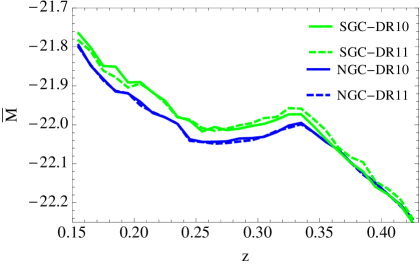
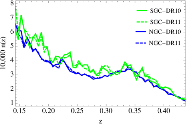
In the top panel of Figure 3 we show the average absolute magnitude of the (k-corrected r-band) galaxies in the LOWZ sample for DR10 and DR11. We see that the average magnitude of the sample varies with redshift for both the NGC or SGC. Moreover the shape as a function of redshift is similar to that of the number density, which we show in the bottom panel of Figure 3. This suggests that the HOD parameters are not likely to be well approximated as constant with redshift.

In this paper we want to improve on the mocks by allowing the HOD parameters to vary as a function of redshift. Fitting a different HOD pareametes in redshift slices would not constrain the HOD parameters sufficiently, so we have chosen instead to include the redshift dependence through a fixed dependency of the HOD parameters on the number density of galaxies. This dependency is based on previous studies, as we now describe.

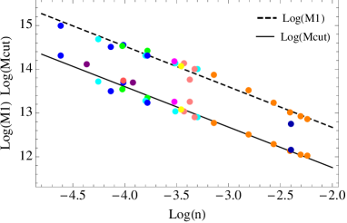
Parejko et al. (2013) report a compilation of the Mcut and M1 HOD parameters from various papers in the literature based on a variety of different galaxy samples. While the functional form of the HOD used in these papers varies, they are sufficiently similar to allow for a comparison between the derived parameters and thus study the evolution of the HOD. We have used the data from Table A1 in Parejko et al. (2013)to fit a log-linear dependence of Mcut and M1 as a function of the number density of galaxies used in each paper. In Figure 4, we show the data and our best fits,

$$\textrm{log}M_{cut} = \textrm{log}M_{cut}^{0}+S_{cut}\bar{n}\;,$$

$$\textrm{log}M_{1} = \textrm{log}M_{1}^{0}+S_{1}\bar{n}\;,$$ (7)

where $\textrm{log}M_{cut}^{0}=9.90\pm 0.12$, $S_{cut}=-0.925\pm 0.035$, $\textrm{log}M_{1}^{0}=10.81\pm 0.12$ and $S_{1}=0.928\pm 0.037$.

We have considered data from publications that include the parameters $\alpha$, $\kappa=M_{0}/M1$, or $\sigma_{logM}$, and found no significant dependency of these parameters on the number density of galaxies. Consequently, when fitting the HOD parameters for our mocks, we keep these parameters constant as a function of redshift, while for $M_{cut}$ and $M_{1}$ we have fixed the tilts $S_{cut}$ and $S_{1}$ to the best fit values given the previous data and fitted only the amplitudes $M^{0}_{cut}$ and $M^{0}_{1}$ to the BOSS data. For a redshift and luminosity depenence of the HOD see also Zheng et al. (2007); Coupon et al. (2012); Tinker et al. (2013); Hong et al. (2014).

4.2 Fit to n(z)

The actual number density of observed LOWZ galaxies varies as a function of redshift for two main reasons. The principal effect is due to the color and magnitude cuts of the target selection that induce a smooth redshift dependence. In addition, there are ’high-frequency’ variantions in redshift that come from observing a particular volume of the universe, i.e, cosmic variance. The shot-noise contribution from being a sample with a finite number of galaxies is subdominant respect to the cosmic variance.

We creating our suit of mock catalogues, we aim to an average redshift distribution that matches the smooth component of the observed redshift profile without the noisy component that is specific to the observed sample. The noisy contribution is accounted for as each mock is a different realization of our universe, within our fiducial cosmology.

Figure 4: HOD parameters $M_{cut}$ and $M_{1}$ as a function of the number density of galaxies. The points are from the list of table A1 in Parejko et al. (2013). Blue: SDSS LRG (2PCF), Zheng et al. (2009); Mandelbaum et al. (2006); Cyan: SDSS LRG (Photo-z, BCL), Blake et al. (2008); Pink: SDSS LRG (Photo-z, PW), Padmanabhan et al. (2009); Dark Blue: Combo-17 Phleps et al. (2006); Purple: SDSS LRG (Lensing), Mandelbaum et al. (2006); Red: SDSS LRG (3PCF),Kulkarni et al. (2007); Orange: NDWFS, Brown et al. (2008); Green: 2SLAQ Wate et al. (2008); Kulkarni et al. (2007); Yellow: BOSS CMASS, White et al. (2011); Magenta: LOWZ Parejko et al. (2013)

We have therefore smoothed the observational galaxy redshift distribtuion to obtain the target n(z) to which we fit the HOD of the mock galaxy catalogues. The smoothed n(z) is a cubic spline curve with seven nodes. The number of nodes and their n(z) values have been determined with a minimization process. First, we have estimated a covariance matrix of n(z), in bins of 0.05, from a preliminary version of the mocks that already included a redshift dependent number density. Then, using this covariance matrix, we have fitted a set of cubic splines to the observed n(z), each spline with a different number of nodes. For each of these splines we have set the n(z) values by minimising the $\chi^{2}$ against the observed n(z). As expected the goodness of fit increases with the number of nodes but at the expense of mimicking all the little wiggles that are inducced by cosmic variance. Consequently, we have used the lower number of nodes that fit the data with $\chi^{2}\sim 1$ per degree of freedom.

We have found that, for the NGC, seven nodes between $0.1175<z<0.4425$ fit well the redshift distribution, so we have used this number for our n(z) spline. The redshift range is broader than the one we use for our LOWZ sample $0.15<z<0.43$ to allow for redshift space distortions that may cross the redshift boundary. We have fitted the SGC with the same number of nodes, as we expect the smooth component of n(z) to be similar in the two hemispheres and the NGC measured n(z) has a higher signal-to-noise (see (Tojeiro et al., 2013) for a discussion of NGC and SGC differences).

Figure 5: Number density of galaxies of the LOWZ DR10 galaxy sample for the NGC (blue dots, lower values) and the SGC (green dots, higher values). Error bars show the rms of the 1000 mock galaxy catalogues. The solid lines are fits to the data. The mock galaxy catalogues n(z) are shown in dashed lines; all the redshift dependence of the mocks n(z) comes through the variation of the HOD.

We have set the HOD parameters by minimizing the $\chi^{2}$ value of the power spectrum and the number density. The joint $\chi^{2}$ is thus the addition of the two respective contributions:

$$\begin{split}\chi^{2}=\sum_{i,j}(P^{m}(k_{i})-P^{d}(k_{i}))C_{i,j}(P)^{-1}(P(k_{j})^{m}-P(k_{j})^{d})\\ +\sum_{st}(n^{m}(z_{s})-n^{d}(z_{s}))C_{s,t}(n)^{-1}(n(z_{t})^{m}-n(z_{t})^{d}),\end{split}$$ (8)

where $P(k_{l})$ is the value of the power spectrum at wave number bin $l$, and $C_{i,j}(P)$ is the covariance matrix of the power spectrum. In the same manner $n(z_{l})$ is the value of the number density at redshift bin $l$, and $C_{s,t}(n)$ the covariance of the number density of galaxies. The labels $d$ and $m$ stand for data and mocks. We have fitted $P(k)$ in the range $0.02<k<0.15$ and $n(z)$ in the range $0.15<z<0.43$. For each HOD set of parameters that we have run we took the mock power spectrum and number density to be the mean of ten realizations for the NGC and twenty for the SGC. In this way we reduce the effect of fiting the data with only one mock catalogue. We have used twenty mocks for the SGC and then for the NGC in order to have a similar number of galaxies in both cases.

To minimize the $\chi^{2}$ we have used the simplex algorithm of Nedler and Mead (1969). This method constructs a multi-dimensional simplex with vertices given by the initial guess of the HOD parameters and a certain step-size. By a series changes of the position of the vertex with worst $\chi^{2}$ the simplex moves in the parameter space until it brackets the minimum within a given volume.

For the covariance matrices we have used an estimation of a preliminary version of the mocks that had been created in the same manner starting with the HOD parameters of Parejko et al. (2013). With this covariance matrix we then minimized the HOD, separately for the NGC and SGC, obtaining the following best fits:

param	NGC	SCG
$\textrm{log}M_{cut}$	13.20	13.14
$\textrm{log}M_{1}$	14.32	14.58
$\textrm{log}M_{0}$	13.24	13.43
$\sigma_{logM}$	0.62	0.55
$\alpha$	0.93	0.93
$\chi^{2}$	49	30

Table 2. HOD values for the LOWZ mock catalogues.

where $\textrm{log}M_{cut}$, $\textrm{log}M_{1}$ and $\textrm{log}M_{0}$ are the values of these parameters when in Eq (7) we set $n(z)=2.98\cdot 10^{-4}$ and $S_{cut}$ and $S_{1}$ are respectively $-0.925$ and $-0.928$.

As the HOD that we are using has five free parameters there is some room for the best fit to vary depending on the initial guess at which the fiting starts as well as the particular set mock realizations used to fit the data. We also expect the observational HOD to be different due to the fact that 7 per cent of our galaxies are not in resolved halos in our simulation. The values we have found for the HOD parameters are within one sigma of the mean of the full sample in Parejko et al. (2013). The recovered $\chi^{2}$ values for our best-fit HOD models show they are a good fit to the data. Indeed, since we have 88 bins in total (32 from $P(k)$ and 56 from $n(z)$), the $\chi^{2}$ square values are less than the number of degrees of freedom, and thus a good fit for the purposes of creating mocks for covariance matrices and clustering data analysis.

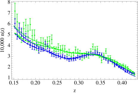
In Figure 5 we show the number density of galaxies in the DR10 LOWZ sample for the NGC and the SGC, with errors displaying the rms of the 1000 mock catalogues. The solid lines show the mean of the targeted n(z) that comes from the seven-node spline fit to the data, and the dashed lines shows the mean n(z) of the mock galaxy catalogues. The number density of the mocks have not been subsampled and its redshift dependence comes only through Eq (7) after fitting for the HOD parameters. We recover the redshift distribution for $z>0.2$ quite well. At lower redshift the differences come from the fact that the log-linear (or constant) dependence of the HOD mass parameters as a function of n(z) is an aproximation to the true HOD as function of redshift.

Following the methods outlined in Sections 3 and 4 we have created one thousand mock galaxy catalogues for the LOWZ DR10 and DR11 galaxy sample. Since both releases have the same targeting their clustering and redshift distributions are very similar. We have consequently used the same halo fields and HOD parameters for both releases, those fitted with DR10 data.

5 Results

Figure 6: Power spectrum and correlation function of the LOWZ galaxy sample. The DR10 NGC and SGC measurements are shown as blue solid circles and green solid triangles respectively, with sample errors from the dispersion of the mock galaxy catalogues. DR11 clustering is displayed in open symbols. The mean values of the mock catalogues are shown for the NGC and SGC as blue and red lines.

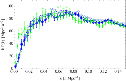
In the left panel of Figure 6 we show the power spectrum of the DR10 LOWZ galaxy sample with errors from the mocks, both for the NGC (blue solid circles) and the SGC (green solid circles). The DR11 values are set as open symbols. We have used the Feldman, Kaiser & Peacock (1994) (FKP) estimator. The mean of the mock catalogues is shown by the solid lines. There is a good fit between the data and the mock catalogues for $k>0.02$, which is the region in which we have fitted the HOD. At lower $k$ values the power of the mock catalogues decreases, as expected for any $\Lambda$CDM cosmology with typical values from WMAP or PLANCK measurements. The power of the DR10 galaxy sample for the NGC decreases as well, but the SGC increases having extra power compared to the NGC. Tojeiro et al. (2013) have looked at the differences between NGC and SGC data in terms of systematics and found that none of the systematic contributions analysed in the CMASS sample has an significant impact in the LOWZ data. Tojeiro et al. (2013) found that the differences between the two galactic caps are reduced in DR11 and are compatible with one another, given the expected variance computed from the mocks.

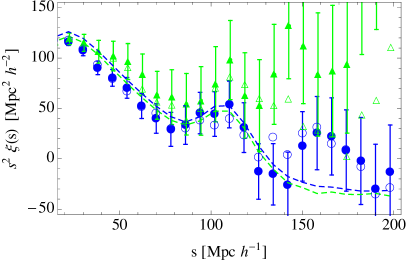
In the right panel of Figure 6 we show the two-point correlation function of the DR10 LOWZ galaxy sample both for the NGC (blue solid circles) and SGC (green solid). The DR11 values are set as open circles. We have used the Landy & Szalay (1993) estimator, including FKP weights as it reduces the variance also in the correlation function. The error bars are the sample errors computed from the mock catalogues and the values of the mean of the mocks are shown as solid lines. The excess power of the SGC at low $k$ translates into a higher values of the correlation function at a wide range of scales.

We present the values of the DR10 LOWZ power spectrum and correlation function, and their covariance matrices in the appendix of the paper. The mocks for LOWZ DR10 will be made publicly available online. These mocks have been used by the BOSS collaboration in analysis of the large scale of the LOWZ sample and the BAO peak position (Anderson et al., 2013; Tojeiro et al., 2013; Sanchez et al., 2013). The elements of covariance matrices estimated from a finite set of mocks have uncertainties that depend on the number of mocks. These uncertainties translate into errors in the inverse covariance matrices and likelihood estimators. Since our suit consists of 1000 mocks these errors are expected to be small in most cases, and are of order few percent for 1000 mocks using $~{}30$ bins. For a detailed accounting for this errors see Percival et al. (2013).

6 Conclusion

We have created 1000 mock galaxy catalogues for the BOSS LOWZ DR10 and DR11 galaxy sample. These mock catalogues have been produced following the PTHalos method developed in Manera et al. (2013), but with significant differences. We have created 500 particle dark matter fields using a 2LPT code and obtained halos in those fields by FoF method with the appropriate linking length. The mass of the halos have been ranked and masses re-assigned to match the Tinker et al. (2008). These PTHalos have been populated with galaxies. For each matter field we can fit two full LOWZ footprints without overlap, resulting in a 1000 mocks for both the Northern Galactic Cap and the Southern Galactic Cap. Redshift space distortions are included through peculiar velocities.

In contrast to previous mocks these have been created allowing for a variable HOD as a function of redshift, authomatically matching the number density of galaxies. The mocks were created by fitting simultanously the measured clustering and number density, with no need for applying a posterior subsampling of galaxies. We have implemented the DR10 and DR11 LOWZ masks to the mock catalogues, including small vetoed areas due to bright stars or other effects like bad photometry and target completeness. We have also included close pair corrections, and redshift failures. For the fitting procedure and HOD dependence on number density see Section 4. The one thousand LOWZ mocks galaxy catalogues have been used in the analysis of the Baryon Accoustic Peak position Anderson et al. (2013) and shape of the correlation function Sanchez et al. (2013). In the appendix we present the LOWZ DR10 correlation function covariance matrix.

Mock galaxy catalogues for the BOSS CMASS galaxy sample ($0.43<z<0.7$) have also been upgraded from DR9 Manera et al. (2013) to DR10 and DR11, keeping the same HOD but repopulating the halos and applying the DR10 and DR11 footprints, completeness masks, and $n(z)$ fit as in Section 3. These mocks have been used in studying the clustering of red and blue galaxies, (Ross et al., 2012) the accuracy of fitting methods (Vargas-Magana et al., 2013) and the analysis of the the large scale clustering and its cosmological implications, including the BAO position, anisotropic clustering (Anderson et al., 2013; Samushia et al., 2013b; Sanchez et al., 2013; Chuang et al., 2013).

The DR10 LOWZ and CMASS mocks will be publicly available online.⁵

C(r1,r2)	30	38	46	54	62	70	78	86
30	32.15
38	23.15	21.58
46	15.69	15.86	15.52
54	11.29	11.69	12.27	12.37
62	8.384	8.821	9.545	10.12	10.42
70	6.186	6.786	7.479	8.015	8.698	8.879
78	5.013	5.452	6.112	6.504	7.085	7.511	7.74
86	4.142	4.437	4.936	5.268	5.718	6.068	6.576	6.736
94	3.112	3.244	3.691	3.97	4.303	4.587	5.091	5.475
102	2.479	2.526	2.88	2.978	3.251	3.542	3.976	4.306
110	2.118	2.019	2.175	2.223	2.419	2.674	2.967	3.209
118	1.544	1.516	1.66	1.694	1.808	1.962	2.158	2.352
126	1.068	1.204	1.341	1.376	1.406	1.572	1.737	1.878
134	0.7244	0.8605	1.002	1.04	1.028	1.205	1.367	1.451
142	0.445	0.6053	0.7028	0.755	0.7507	0.8816	1.004	1.054
150	0.2411	0.387	0.4769	0.539	0.5401	0.6727	0.788	0.8107
C(r1,r2)	94	102	110	118	126	134	142	150
94	5.405
102	4.453	4.527
110	3.355	3.634	3.697
118	2.456	2.735	2.996	3.145
126	1.933	2.151	2.464	2.743	3.013
134	1.505	1.675	1.965	2.257	2.625	2.874
142	1.142	1.267	1.511	1.745	2.081	2.435	2.595
150	0.9066	0.9725	1.175	1.364	1.655	1.987	2.224	2.351

C(r1,r2)	30	38	46	54	62	70	78	86
30	88.16
38	64.43	60.73
46	46.3	47.45	48.32
54	31.59	34.57	37.63	37.47
62	22.36	24.87	27.6	28.97	27.87
70	16.61	18.52	20.92	22.38	22.84	23.49
78	12.62	14.	15.86	17.49	18.24	19.44	19.94
86	10.01	11.11	12.17	13.61	14.06	15.13	16.58	17.06
94	7.674	8.367	8.902	10.17	10.58	11.59	12.97	14.26
102	5.459	5.619	5.887	7.01	7.602	8.493	9.906	11.18
110	4.166	3.76	3.783	4.482	5.065	5.691	6.794	7.997
118	3.224	3.056	3.02	3.224	3.587	3.975	4.75	5.717
126	2.576	2.477	2.275	2.214	2.578	2.94	3.514	4.247
134	1.27	1.109	1.153	1.215	1.705	2.064	2.476	3.051
142	0.004535	0.03784	0.3373	0.5719	1.084	1.364	1.764	2.213
150	-0.9506	-0.5445	-0.04525	0.1988	0.6778	1.04	1.389	1.789
C(r1,r2)	94	102	110	118	126	134	142	150
94	14.88
102	12.37	12.9
110	9.248	10.35	10.57
118	6.905	8.08	8.722	9.293
126	5.098	6.116	6.719	7.655	8.256
134	3.662	4.599	5.144	6.05	6.983	7.645
142	2.589	3.244	3.643	4.449	5.385	6.302	6.868
150	2.005	2.394	2.605	3.227	4.12	4.917	5.789	6.43

Table 2: Covariance matrices of the spherically averaged correlation function $\xi(s)$ for the LOWZ DR10 NGC (top) and SGC (bottom), derived from one thousand mock galagxy catalogues. The first column and the lines with integers indicate the center of the bins in h^-1 Mpc. Since the covariance matrix is symmetric only the lower half is displayed, and its values, for clarity, multiplied by $10^{6}$.

References

- Abell et al. (2009) Abell P.A., Allison J., Anderson S.F, Andrew J.R., Angel J.R.P., et al., 2009, arXiv 0912.0201
- Anderson et al. (2012) Anderson L., et al., 2012, MNRAS, 427, 3435 [arxiv:1203.6594]
- Anderson et al. (2013) Anderson et al., 2013, BOSS collaboration paper, arXiv:1312.4877
- Angulo et al. (2013) Angulo, Raul E.; Baugh, Carlton M.; Frenk, Carlos S.; Lacey, Cedric G., 2013, eprint arXiv:1310.3880
- Blake et al. (2008) Blake C., Collister A., Lahav O., 2008, MNRAS, 385, 1257
- Blake et al. (2011) Blake, C.; David, D.; Poole, G.G; Parkinson, D., 2011, MNRAS, 415, 2892-2909
- Brown et al. (2008) Brown M. J. I. et al., 2008, ApJ, 682, 937
- Bryan and Norman (1998) Bryan G.L and Norman M.L, 1998, ApJ 4095, 80
- Coupon et al. (2012) Coupon, J.; Kilbinger, M.; McCracken, H. J.; Ilbert, O.; Arnouts, S.; Mellier, Y.; Abbas, U.; de la Torre, S.; Goranova, Y.; Hudelot, P.; Kneib, J.-P.; Le F vre, O., A& A (2012) 542, 5
- Chuang et al. (2013) Chuang, Chia-Hsun, et al., arXiv:1312.4889
- Davis et al. (1985) Davis M., Efstathiou G., Frenk C.S., White S.D.M., 1985, ApJ, 292, 371
- Dawson et al. (2013) Dawson K. S., et al., 2013, AJ, 145, 10
- de la Torre & Peacock (2013) de la Torre, Sylvain; Peacock, John A., 2013, MNRAS, 435, 743
- Eisenstein et al. (2001) Eisenstein D. J., et al., 2001, AJ, 122, 2267
- Eisenstein et al. (2011) Eisenstein D.J., et al., 2011, AJ 142, 72
- Feldman, Kaiser & Peacock (1994) Feldman H.A., Kaiser N., Peacock J.A., 1994, ApJ, 426, 23
- Hill et al. (2004) Hill, G. J.; Gebhardt, K.; Komatsu, E; MacQueen, P.J., The New Cosmology: Conference on Strings and Cosmology; The Mitchell Symposium on Observational Cosmology, AIP Conference Proc., 743, 2004, p.224-233
- Hong et al. (2014) Hong Guo Zheng Zheng, Idit Zehavi, David H. Weinberg, in prep
- Kitaura and He (2013) Kitaura, Francisco-Shu and He , Steffen, 2013, MNRAS Letters, 435, L78
- Kulkarni et al. (2007) Kulkarni G.V., Nichol R.C., Sheth R.K., Seo H., Eisenstein D.J. and Gray A., 2007, MNRAS 378, 1196K
- Landy & Szalay (1993) Landy S.D., Szalay A.S., 1993, ApJ 412, 64
- Laurejis et al. (2011) Laurejis R., Amiaux J., Ardunini S., Auguères J., et al., 2011, arXiv:1110.3193
- Levi et al. (2013) Levi, Michael; Bebek, Chris; Beers, Timothy; Blum, Robert; Cahn, Robert; Eisenstein, Daniel; Flaugher, Brenna; Honscheid, Klaus; Kron, Richard; Lahav, Ofer; McDonald, Patrick; Roe, Natalie; Schlegel, David; representing the DESI collaboration, 2013, arXiv:1308.0847
- Mandelbaum et al. (2006) Mandelbaum R., Seljak U., Kauffmann G., Hirata C. M., Brinkmann J., 2006, MNRAS, 368, 715
- Manera et al. (2013) Manera M., Soccimarro R., Percival W. J., et al., 2013, MNRAS 428, 1036-1056
- McBride et al. (2013 in prep) McBride C., 2013, in preparation. http://lss.phy.vanderbilt.edu/lasdamas/download.html
- Monaco et al. (2013) Monaco, P.; Sefusatti, E.; Borgani, S.; Crocce, M.; Fosalba, P.; Sheth, R. K.; Theuns, T., 2013,MNRAS, 433, 2389
- Monaco et al. (2002) Monaco, P., Theuns, T., & Taffoni, G. 2002, MNRAS, 331, 587
- Parejko et al. (2013) Parejko J. K., Sunayama T., Padmanabhan N., Wake D., Berlind A.A., Bizyaev D., Blanton M., Bolton A., et al., 2013, MNRAS, 529, I1 p98-112
- Padmanabhan et al. (2009) Padmanabhan N., White M., Norberg P., Porciani C., 2009, MNRAS, 397, 186
- Percival et al. (2013) Percival W.J., et al. 2013, submitted to MNRAS
- Phleps et al. (2006) Phleps S., Peacock J. A., Meisenheimer K., Wolf C., 2006, A&A, 457, 145
- Reid et al. (2012) Reid B., Samushia L., White M., et al., MNRAS, 2012, 426, 2179
- Ross et al. (2012) Ross A.J., et al., 2013, submitted to MNRAS
- Samushia et al. (2013a) Samushia L., Reid B., White M., et. a., 2013, 429, 1514
- Samushia et al. (2013b) Samushia L., submitted to MNRAS, arXiv:1312.4899
- Sanchez et al. (2013) Sánchez A.G., 2013, submitted to MNRAS, arXiv:1312.4854
- Scoccimarro and Sheth (2002) Scoccimarro R., Sheth R.K, 2002, MNRAS 329, 629
- Tassev et al. (2013) Tassev, Svetlin; Zaldarriaga, Matias; Eisenstein, Daniel J., 2013, JCAP, 06, 036
- Tinker et al. (2008) Tinker, J.L., Kravtsov, A.V., Klypin, A., Abazajian, K., Warren, M.S., Yepes, G., Gottloeber, S., Holz, D.E., 2008, ApJ, 688, 709
- Tinker et al. (2013) Tinker, Jeremy L.; Leauthaud, Alexie; Bundy, Kevin; George, Matthew R.; Behroozi, Peter; Massey, Richard; Rhodes, Jason; Wechsler, Risa H., ApJ (2013) 778, 93
- Tojeiro et al. (2013) Tojeiro R., et al., 2013, LOWZ galaxy sample
- Tojeiro et al. (2012) Tojeiro R., et al., MNRAS (2012) 424, 2339
- Vargas-Magana et al. (2013) Vargas-Magana M., 2013, arXiv:XXXX.XXXX
- Wate et al. (2008) Wake D. et al., 2008, MNRAS, 387, 1045
- White et al. (2011) White, Martin; Blanton, M.; Bolton, A.; Schlegel, D.; Tinker J.; et al., ApJ 728 (2011) Issue 2, 126
- White et al. (2013) White M., Tinker, J.L, and McBride, C, 2013, MNRAS online
- Xu et al. (2012) Xu X., Cuesta A.,J., Padmanabhan N, Eisenstein D.J., and McBride C., 2013, MNRAS 431,2834
- Zheng et al. (2009) Zheng Z., Zehavi I., Eisenstein D. J., Weinberg D. H., Jing Y. P., 2009, ApJ,707, 554
- Zheng et al. (2007) Zheng, Zheng; Coil, Alison L.; Zehavi, Idit, Apj (2007) 667,760