Cosmological Parameter Uncertainties from SALT-II Type Ia Supernova Light Curve Models
Abstract
We use simulated type Ia supernova (SN Ia) samples, including both photometry and spectra, to perform the first direct validation of cosmology analysis using the SALT-II light curve model. This validation includes residuals from the light curve training process, systematic biases in SN Ia distance measurements, and a bias on the dark energy equation of state parameter . Using the SN-analysis package SNANA, we simulate and analyze realistic samples corresponding to the data samples used in the SNLS3 analysis: low-redshift () SNe Ia, SDSS SNe Ia (), and SNLS SNe Ia (). To probe systematic uncertainties in detail, we vary the input spectral model, the model of intrinsic scatter, and the smoothing (i.e., regularization) parameters used during the SALT-II model training. Using realistic intrinsic scatter models results in a slight bias in the ultraviolet portion of the trained SALT-II model, and biases () ranging from to . These biases are indistinguishable from each other within the uncertainty; the average bias on is .
1. Introduction
In 1998, observations of type Ia supernovae (SNe Ia) revealed the accelerating expansion of the universe (Riess et al., 1998; Perlmutter et al., 1999), attributable to an unknown source of acceleration commonly called “dark energy.” SNe Ia based measurements allow the direct detection of dark energy, and as such remain valuable components of the quest to understand this mysterious phenomenon. In particular, over the past decade observational cosmology has focused on measuring the cosmological equation of state parameter (e.g., Weinberg et al., 2013).
The cosmological utility of SNe Ia is due to their nature as standardizable candles. Building on work by Pskovskii (1977), Phillips (1993) was the first to demonstrate that shapes of SN Ia light curves are correlated with their absolute luminosity. An additional correlation between SN Ia color and luminosity was shown by Tripp (1998), resulting in a two-parameter luminosity correction. Although other standardization methods exist, including infrared light curve shapes (Barone-Nugent et al., 2012; Kattner et al., 2012) and spectral ratios (e.g., Bailey et al., 2009), the ubiquity of optical SN Ia light curve data makes shape and color standardization the most common technique.
SN light curve analysis is the process of empirically training an SN model with broadband photometry and spectra, using the model to determine the SN light curve shape and color information, and deriving the best possible distance measurements from these SN parameters. SN light curve analysis is one source of systematic uncertainty affecting our ability to constrain the nature of dark energy.
A thorough study of systematic uncertainties arising from SN light curve analysis has been made by Guy et al. (2010) (hereafter G10) specifically regarding the training of the SALT-II light curve model and its application to the 3-year Supernova Legacy Survey (SNLS) SN Ia cosmology sample (Conley et al., 2011). To quantify systematic uncertainties in SN Ia distance measurements, G10 uses two main techniques: calculations and variation analysis. For instance, calculations are used to determine the model statistical uncertainties from the training covariance matrix, and variations are used to estimate uncertainties due to light curve model training procedures.
The key results of these tests — distance uncertainties as a function of redshift — are shown in G10(Figure 16). In general, G10 finds light curve model-related fluctuations about the fiducial result to be small, with at most redshifts. However, because these results are based on a limited training sample and test set, it is not clear that these results would hold in general for any training sample and test set. Nor is it possible to determine whether the distances themselves (and the associated cosmology parameter ) are biased.
In this paper, we use detailed Monte Carlo (MC) simulations to reevaluate the systematic uncertainties determined by G10 for SALT-II and the 3-year SNLS cosmology sample. In addition, the large statistics afforded by simulations allow us to rigorously determine biases in the Hubble Diagram (HD) and resulting from the full SN light curve analysis procedure.
SN Ia modeling consists of a set of assumptions about the number of observable SN Ia parameters. As mentioned above, most SN Ia models assume that the family of SNe Ia may be described by two parameters – light curve shape and color. Models define the SN Ia rest frame flux as a function of phase (rest-frame days since peak -band magnitude), wavelength, and observable light curve parameters. Since SN Ia progenitors and explosion mechanisms remain ill-defined, models are empirically determined and must be “trained” from a subset of observed SN data for which initial light curve parameter values can be estimated. The training procedure consists of solving for the model parameters that best fit the training set of observed SN Ia data. For example, training of the magnitude-based MLCS2k2 model (Jha et al., 2007) includes solving for bandpass-dependent coefficients which relate magnitudes to light curve shapes. The training of the flux-based model SALT-II (Guy et al., 2007) includes solving for the coefficients of the spline basis functions used to represent SN Ia flux as a function of wavelength and phase.
Once the best-fit model parameters have been found, the model is ready to be used for light curve fitting. For each SN in the data set, the trained model is used to compute synthetic observed magnitudes in conjunction with minimization routines to “fit” the most likely light curve parameters (e.g., stretch , color , and an overall normalization factor ). With the data set light curve parameters in hand, distances may be calculated and an HD constructed for cosmological parameter determination.
Currently, the main source of the SN Ia HD systematic uncertainty is photometric calibration (e.g., Sullivan et al., 2011). However, improved low-redshift SN Ia samples (Hicken et al., 2009; Holtzman et al., 2008; Stritzinger et al., 2011) and greater attention to calibration (e.g., Betoule et al., 2013) are reducing the significance of this contribution, making it increasingly important to understand systematic uncertainties related to the training and implementation of the light curve model itself. Because the same trained model is used to fit all SN light curves, the model’s statistical uncertainties introduce correlated uncertainties into the fitted light curve parameters.
The SN Ia model, training procedure, and training set are all sources of uncertainties that affect light curve parameter measurement, and hence cosmology parameter measurement. One approach to determine model-related systematic uncertainties is to compare cosmology results from the same set of SN Ia observations evaluated with different SN Ia models. The most notable studies of model-related systematic uncertainties have been undertaken by Kessler et al. (2009a) (K09), comparing the MLCS2k2 and SALT-II models, and G10, comparing SALT-II and SiFTO (Conley et al., 2008). K09 found a significant difference between MLCS2k2 and SALT-II derived cosmology parameters, which they attributed to the different handling of color in the two models and the fact that MLCS2k2 training is much more reliant on observer-frame observations in the ultraviolet region. G10 found that SALT-II and SiFTO produced similar cosmology results.
A second technique is to estimate light curve model-based distance uncertainties directly from the model training itself. G10 take this approach to estimate the sizes of systematic distance uncertainties caused by 1) finite training samples and 2) the wavelength dependence of the scatter between the model and the training data. As shown in Figure 16 of G10, these uncertainties have been estimated as a function of redshift for the SALT-II model.
While these two approaches are used to estimate the model uncertainty, the true model bias cannot be determined from SN Ia observations. Therefore it is possible that systematic offsets in the trained model parameters may propagate as-yet unknown biases onto the final HD. Properly determining these biases is the focus of this work and will be instrumental to correctly interpreting SN Ia cosmology data, constructing future training sets, and designing the next generation of SN Ia models.
1.1. Training Test Overview
In this work we use simulated SN Ia samples to directly evaluate systematic biases and uncertainties originating from the SN Ia light curve analysis, with a specific focus on model training and bias corrections. We use the SALT-II model exclusively: the most recent, most precise SN Ia cosmology results are based on SALT-II light curve fits (Sullivan et al., 2011), making this state-of-the-art model an ideal choice for these systematics studies. In addition, its automated training process makes it straightforward to generate the multiple training iterations needed to evaluate biases.
By examining such quantities as training residuals, Hubble residuals,
and best-fit cosmologies resulting from various training configurations
and input training sets we will answer three key questions about SALT-II.
First, we will test the ability of the SALT-II framework to determine the model
uncertainty from input data.
Second, we will quantify the biases in Hubble residuals and cosmology parameters
caused by “regularization”, the training strategy used to manage phase or wavelength gaps in the training data.
Third, we will measure biases resulting from mismatches between the underlying
model and the assumed SALT-II model.
Figure 1 provides an overview of the process this work uses to test SALT-II training.
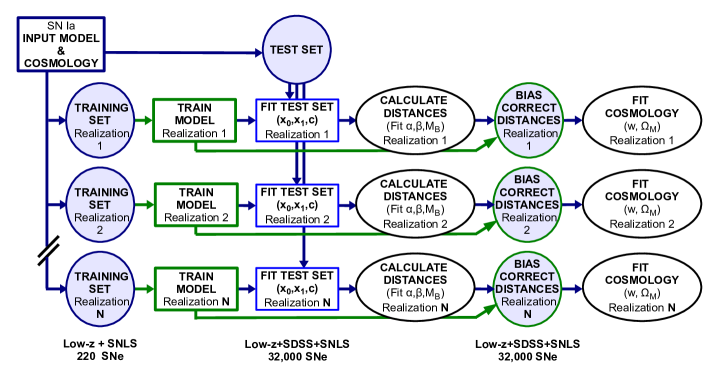
From an SN Ia input model and cosmology, statistically independent realizations of SN Ia training sets (light curve photometry and spectra) are generated. These observations (“Training Sets”) are used to train new SALT-II models (“Trained Models”). Finally, each trained model is used to fit a single set of SN Ia light curves (“Test Set”) generated from the SN Ia input model, resulting in sets of light curve parameters ().
We have adapted existing SN Ia MC simulation routines from the SN analysis software package SNANA (Kessler et al., 2009b) to enable accurate random realizations of both the light curve photometry and spectral data samples forming the basis of the most recent published SALT-II model training. There are two key parts to this change. First, we have added a spectral simulation component, which uses an SN Ia spectral energy distribution (SED) model and a library of existing SN Ia spectral observations to produce spectra with realistic signal-to-noise ratios, resolution, cadences, wavelength coverage, and galaxy contamination. Second, we have added several new intrinsic scatter models (described in K13), as well as the machinery to apply them to simulated light curves and spectra.
In addition to measuring biases introduced by the training, our multiple training set realizations are used to check estimates of the statistical uncertainty of SALT-II model parameters due to the finite sizes of existing training sets and directly measure uncertainties resulting from different choices of training parameters.
Most importantly, because the underlying cosmology and parameter distributions of the simulated training sets are known, we are able to perform complete light curve analyses for each set of input models, from model training through HD construction and cosmology fits. We use this information to evaluate HD bias as a function of redshift, and biases in . This is the first systematic study in which simulations are used to directly test uncertainties and biases resulting from SN Ia light curve analysis. The software used to run these light curve analysis tests is part of the publicly available SNANA supernova software package; these tools can be adapted to test other SN Ia models and data samples.
The outline of the paper is as follows. A brief introduction to the SALT-II model and its training procedure will be given in Section 2. Section 3 details the input SN Ia models which will be used for this work, followed by a discussion of our simulations and data analysis procedures, including redshift-dependent bias corrections, in Section 4. Section 5 describes the metrics with which training results will be evaluated. Section 6 presents results of our two main training tests: trainings with idealized training sets and trainings with realistic training sets. Finally, the implications of the results of these tests for further SALT-II training, light curve model development, and training set observations are described in Section 7.
2. Training SALT-II
The SALT-II model describes SNe Ia with three components: two spectral time series and , and a color law CL. The component is identified as the mean SN Ia SED; component accounts for light curve width variations. The color law CL incorporates any wavelength-dependent color variations that are independent of epoch. No assumptions about dust or extinction laws are made a priori. These three components are assumed to be the same for all supernovae. The flux for an individual SN Ia is determined by the components described above and three supernova-specific parameters: the overall flux scale , the light curve shape parameter , and the peak color . As a function of phase and wavelength the flux is:
| (1) |
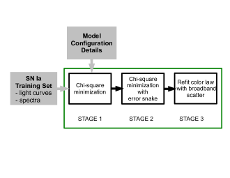
More details on the SALT-II model may be found in Guy et al. (2007) and G10. A cartoon schematic of the SALT-II training process is shown in Figure 2. The SALT-II model parameters and are presented in Sections 2.1-2.3. Descriptions of the additional model uncertainties used to account for SN Ia intrinsic variability are given in Section 2.4.
2.1. SALT-II Model Parameters
Defining to be the set of model parameters, solving for the best-fit model consists of varying to minimize the chi-squared () corresponding to the difference between the training set SN fluxes, , and corresponding model fluxes, . Training set fluxes obtained from spectra,, are compared to model fluxes of the same wavelength, , and phase, , adjusted for SN-appropriate recalibration parameters, . Training set fluxes obtained from broadband photometry, , are compared with the integration of the model at phase over the appropriate broadband filter, . In either case, the model is redshifted to match the redshift of the training set SN prior to flux comparison.
The training is:
| (2) |
Here is the set of observable light curve parameters , , for the supernova, is the set of recalibration parameters applied to the spectral flux , and are the statistical uncertainties of the training SN fluxes, and is the uncertainty in the model flux. An extra regularization term , to be discussed in Section 2.3, is also included in the training . The summations are over all spectral and photometric observations of all training set SNe.
Third-order b-spline basis functions are used to construct the and spectral time series. Closely resembling Gaussians, third-order b-spline basis functions are parameterized by knot values, which determine the local region of phase (or wavelength) space to which each basis function contributes, and control points, which determine the amplitude of each basis function. Only the control points are varied during the SALT-II minimization process. The phase range 14 to 50 rest-frame days is spanned by 20 basis functions for a phase resolution of 3.2 days. The wavelength range 2000 to 9200 Å is spanned by 100 splines, or 72 Å per basis function. As in G10, the functional form of the color law is a polynomial with four free coefficients covering the wavelengths 2800 – 7000 Å. The best-fit color law is linearly extrapolated for wavelengths outside these regions.
2.2. Spectral Recalibration
In general, SN Ia spectra are not as well calibrated as SN Ia photometry and spectral flux uncertainties are not uniformly calculated. In order to maximize the benefits of training with heterogeneous spectroscopic data, training set spectra are recalibrated to match the best-fit model of their input light curve data. The recalibration is performed by multiplying each input spectrum by the exponential of a polynomial whose order is determined by the wavelength range of the spectrum and the wavelength coverage of input light curve data. As noted in Equation 2 and Table 1, the polynomial coefficients for each spectrum are part of the best-fit model parameters and are determined iteratively during the minimization process.
2.3. Regularization
If a region of wavelength and phase lacks spectral training data, the corresponding and components are determined by the underlying spline interpolations and constrained solely by broadband photometry. The spline interpolation can produce high-frequency noise or “ringing” in the poorly constrained region. Extra “regularization” terms are added to the training (Equation 2) to disfavor models with unphysical rapid fluctuations in wavelength or phase. However, regularization can also oversmooth, thereby removing real features from the best-fit model.
As described in the Appendix of G10, two types of regularization are used for the SALT-II model: gradient and dyadic. Gradient regularization penalizes changes in flux with respect to wavelength, but ignores changes with respect to phase:
| (3) |
where is the gradient regularizaton weight, is the effective number of spectral flux measurements constraining that region of phase space, and the sums run over all phase and wavelength basis functions.
SALT-II dyadic regularization is implemented as follows:
| (4) |
where is the dyadic regularization weight, is the effective number of spectral flux measurements constraining that region of phase space, and the sums run over all phase and wavelength basis functions. Dyadic regularization favors model fluxes that can be decomposed separately as a function of phase times a function of wavelength (i.e., ).
These terms are combined in the training :
| (5) |
To limit the use of regularizations to those regions that need it the most, we set a cutoff value for : in regions where , . Figure 3 shows as a function of wavelength for four different phase values. Near the epoch of peak luminosity, regularization is not used for wavelengths between 4000 and 8000 Å. On the other hand, most wavelength bins are regularized at early and late times and wavelengths less than 4000 Å are always regularized.
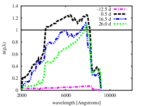
The overall strengths of the regularization terms are controlled by the scaling factors and . Nominal values for these parameters are and .
As an illustration of the importance of the scaling factor values, Figure 4 demonstrates the results of model trainings where and are multiplied by an amount .
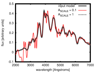
First, we generated a training set and removed all training spectra between phases 2 and 8. Then we ran the nominal SALT-II training twice: once with (i.e., nominal regularization), and once with (i.e., ten times weaker regularization). With the best-fit SALT-II model shows high-frequency oscillations around the input model which increase in amplitude toward the bluest wavelengths. When , the best-fit SALT-II model is almost identical to the input model. Only slight differences in feature strength are evident (e.g. 3000 Å).
The choices of regularization type, scaling factor, and effective number threshold setting are discussed further in Section 6.2.1.
2.4. Intrinsic Variability
To account for intrinsic variability in the SN Ia population the SALT-II model formalism incorporates two additional model uncertainties: a color-independent error scaling factor (hereafter “error snake”) associated with the spectral time series and the parameter, and a broadband magnitude scatter associated with the color law and the parameter. As illustrated by the training schematic shown in Figure 2, the calculation and subsequent incorporation of these added uncertainties require three successive rounds of chi-squared minimization before the final model uncertainty is obtained.111For sake of readability, in this section we have omitted the SN-specific indices and .
After the model best-fit and basis parameters have been determined (“Stage 1” in Figure 2) the error snake is calculated by requiring light curve training data to have reduced chi-squared values of 1 in any given phase-wavelength bin. The default error snake bin size is (6 days) (1200 Å), but it is increased if there are less than 10 data points in each bin. Once the error snake has been calculated, the Stage 1 model uncertainty is redefined as
| (6) |
and the chi-squared minimization is repeated (“Stage 2” in Figure 2). It should be noted that the definition above, which has the error snake scaling the rms, is slightly different from that of Guy et al. (2007) where the error snake scales the model variance.
A similar process takes place for the color law. The SALT-II model formalism assumes a phase-independent broadband magnitude scatter which can be described as a function of the central filter wavelength and a set of parameters such that
| (7) |
The best-fit scatter parameters are determined from the Stage 2 light curve residuals and uncertainties. During this calculation, one free normalization parameter is included for each SN and therefore the coherent contribution to intrinsic scatter is not included in .
Subsequently, the model uncertainty is redefined to include , such that the covariance of two measurements and of the same light curve is
| (8) |
and the final color law is fit (“Stage 3” in Figure 2).
2.5. Final distribution
As discussed in Section 5 of Guy et al. (2007), the average value and scale of the SALT-II stretch parameter are arbitrary. Therefore, the training rescales fitted values to satisfy the distributions and . Although all simulations are performed with global stretch parameter , this rescaling changes the expected value of . Analytic calculations of the expected values as a function of input model are described in Appendix A.
3. SN Ia input models
As illustrated in Figure 1, all training tests begin with the selection of a SN Ia input model. For this work three different input models have been used: the SALT-II surfaces published in G10, a specially designed variant of the SALT-II surfaces published in G10, and a model based on the Hsiao templates (Hsiao et al., 2007). In Sections 3.1-3.3 we describe the motivation for the use of each input model and provide a general description of how the models were made. To match the observed intrinsic scatter, three intrinsic scatter models are combined with each of our input models. Section 3.4 provides details of the intrinsic scatter models we have selected. Finally, Section 3.5 summarizes the model naming conventions used in this work.
3.1. G10 Model
This model is built from the G10 spectral surfaces and the G10 color law, combined as prescribed in Equation (1) for a range of stretch and color values. Because it contains some negative fluxes, especially at early times in the UV region and late times in the near-IR, this model is not suitable for our training purposes; however, it is used for internal cross checks.
3.2. G10′ Model
A second model, hereafter G10′, uses the G10 surfaces as a starting point. To ensure full SALT-II training compatibility, these surfaces were modified to remove negative fluxes, and then translated back onto the desired b-spline training basis. Equation (1) was used to combine the output surfaces with the G10 color law to add color variations.
3.3. H Model
The third type of model we use is based on spectral templates presented in (Hsiao et al., 2007), which we will refer to as the “Hsiao templates.” We use the Hsiao templates because they have real spectral features without being imprinted by an underlying set of basis functions (as is the G10′ model) making this model a useful test of the ability of SALT-II training to reproduce arbitrary SN Ia models. We have added width variation by applying a stretch function to the flux, such that a supernova with stretch and peak time has flux at epoch and wavelength
| (9) |
where . As in the prior two models, the G10 color law was used to add color variation, and the same input range of and values was utilized222From Guy et al. (2007), .
3.4. Intrinsic Scatter Models
Fits of SNe Ia data typically include an intrinsic scatter term on the order of mag, representing the amount of extra uncertainty required to be added in quadrature such that a fit to a SN Ia derived HD obtains a reduced chi-squared value of . Historically, this extra uncertainty has been associated with the peak -band magnitude parameter . However, several recent papers have presented evidence suggesting that the SN Ia scatter varies as a function of wavelength, producing not just magnitude scatter but also color scatter (Guy et al., 2010; Foley & Kasen, 2011; Chotard et al., 2011; Marriner et al., 2011; Kessler et al., 2013; Scolnic et al., 2014) and that the assumptions we make about this scatter affect extinction laws and cosmology derived from our SN data sets. The underlying source of this scatter is a subject of ongoing study. In this work, we use intrinsic scatter models from Kessler et al. (2013) (hereafter K13) to test the effects of different intrinsic scatter forms on SALT-II training. All of the K13 models are defined as wavelength-dependent perturbations to an underlying input model. By design, these perturbations average to zero so that the underlying SN Ia model is not changed. Although all models used in this work are independent of redshift and epoch, the validity of this assumption is not well constrained with current data and remains an active area of research. The chosen models, COH, G10, and C11, are briefly described below. We also employ a model with no intrinsic scatter, which we refer to as “NONE.” As this model is trivial, we omit a description. Combining these intrinsic scatter models with our base H and G10′ models provides eight total input models to choose from.
3.4.1 COH
Coherent magnitude shifts are the simplest form of scatter to add to our base model. For each SN, a shift in flux is chosen from a Gaussian distribution of mean zero and standard deviation equal to the desired scatter ( for this work). The underlying SN Ia flux is multiplied by 1+, then spectra and magnitudes are computed as usual. This scattering model produces a coherent shift in magnitudes; as such it only changes the SN Ia parameter and produces no change in colors.
3.4.2 G10
This scatter model is based on the wavelength-dependent magnitude dispersion measured from the G10 SNLS3 training set during the SALT-II training process (Fig. 8 of G10). To create a perturbation that can be applied to our input models, independent scatter values are chosen from the measured dispersion at 800 Å wavelength intervals and then joined by a sine interpolation. This scattering model produces color scatter as well as magnitude scatter.
3.4.3 C11
Our last scatter model is based on a covariance magnitude scatter model from the Chotard et al. (2011) analysis of high-quality Nearby Supernova Factory spectra. The original scatter model was extended to the UV by K13: we use the C11_0 variant. As with the G10 scatter model, the C11 scatter is determined for broadband wavelengths. To apply it directly to our input models, six correlated random magnitude shifts [] are drawn from the covariance matrix and then connected with the same sine interpolation used for the G10 model. In contrast to the two previous models, the C11 model produces mostly color scatter with minimal magnitude scatter.
3.5. Input Model Naming Conventions
To be clear about which model is being used to train SALT-II, a compound name will be used to describe the input. For example, an input data set created with the G10′ base model altered by G10 scatter will be called G10′–G10, and an input data set created with the H base model altered by COH scatter will be called H–COH. Two additional components are appended to the input model name to signify the types of simulations used (IDEAL or REAL, described in Section 6.1 and 6.2) for the training set and test set simulations. Table 2 summarizes the training option naming conventions used in this work.
| input model | scatter model | training set | test set |
|---|---|---|---|
| H | NONE | IDEAL | IDEAL |
| G10′ | COH | REAL | REAL |
| C11 | |||
| G10 |
Note. — Main training options used in this work. Particular training tests will be identified by a concatenation of options. For instance, a training test based on the H input model with C11 intrinsic scatter trained with an ideal training set and tested on a realistic test set would be designated H-C11-IDEAL-REAL.
4. Simulation and Analysis Methods
As illustrated in Figure 1, using a set of SN Ia light curves and spectra to measure cosmology parameters is a multi-step process. In our case, we begin with an SN Ia model (“INPUT MODEL”) from which we simulate SN Ia training set realizations and a single SN Ia test set. These simulations are the only aspect in which our light curve analysis technique differs from analyses based on real data. Following the order of Figure 1 from left to right, five steps are implemented: (1) the training set is used to train a SALT-II light curve model; (2) the trained light curve model is used to fit the cosmology test set, determining the object-specific model parameters , , for each SN in the set; (3) the ensemble of fitted SN parameters is used to determine global SN Ia parameters , , and . These global parameters are used to calculate the initial SN distances . (4) Redshift-dependent bias corrections are determined and applied to inital distances in order to obtain final distances . (5) Cosmology parameters are determined by fits from the HD. In the following sections we describe the methods used for each of these steps.
4.1. Simulation Overview
As shown by the shaded circles in Figure 1, three different sets of SN Ia simulations are generated as part of our training test procedure: (1) the model training sets, which match real data statistics; (2) the high-statistics SN Ia test set, which represents the data set from which cosmological parameters are measured; (3) the high-statistics bias correction sets. This section provides a brief overview of our simulations. We begin by describing those methods shared by the three sets of simulations, including general simulation techniques and the SN Ia data samples after which our simulations are patterned. Then, we move through our training and test set simulations, describing methods specific to each. Section 4.6.2 presents more information on our bias correction simulations. We close by outlining the tests we have performed to evaluate our simulations.
4.1.1 General Techniques
All of our simulations are performed with the SNANA MC code (Kessler et al., 2009b), and all are based on a flat CDM cosmology with , , , and . SN Ia models may be constructed analytically from a set of model parameters and associated stretch and color parameters (e.g. the SALT-II model, Equation 1), or from a spectral time series lookup table.333The main advantage of a lookup table is to allow arbitrary flexibility in the choice of SN model. Both techniques are used in this work. More details of the latter technique will be given in Section 4.2.
For a given SN Ia simulation, we begin by selecting stretch and color parameter values. Parent distributions of the stretch () and color () parameters are chosen to be asymmetric Gaussians characterized by a mean value and two standard devations and . We choose to use the same stretch and color distributions for all simulated surveys within a given training test, rather than use the separate distributions for each survey that best match the observed data (e.g. K13, Section 3). This choice is made to simplify the interpretation of our training test results.
The goals of this work — to verify the systematic uncertainty estimates of the SALT-II training procedure, to test the impact of regularization on HD biases, and to measure training-related HD bias as a function of redshift — will be satisfied so long as the simulations provide an approximate representation of the data. Comparisons between data and simulations will be presented in Section 4.4.
Once the color and stretch are selected, the SN Ia spectra are generated. All of our SN Ia models are based on time sequences of rest-frame spectra. To generate observer-frame magnitudes for a specific epoch, the appropriate rest-frame spectrum is redshifted and its flux is integrated over the appropriate filter-response curves. To account for non-photometric conditions and varying time intervals between observations due to bad weather, actual observing conditions are used when available. For each simulated observation, the noise is determined from the measured point-spread function (PSF), Poisson noise from the source, and sky background. Contamination from the host-galaxy background is included as needed. The simulated flux in CCD counts is based on the observed mag-to-flux zero points and a random fluctuation drawn from the noise estimate. When available, realistic models of survey search efficiencies are used to determine whether a particular simulated SN Ia epoch would be observed. More details of SNANA light curve simulations can be found in Kessler et al. (2009b) and in Section 6 of Kessler et al. (2009a).
4.1.2 The SN Ia Data Samples
To generate simulated samples similar to the real data used in G10 we pattern our simulations after three key data sets: the SDSS-II sample, the SNLS3 sample, and the nearby sample.
SDSS-II
The SDSS-II SN survey discovered and spectroscopically confirmed 500 type Ia SNe during its three fall operating seasons from 2005–2007 (Frieman et al., 2008). All data were acquired on the SDSS 2.5 m telescope (Gunn et al., 2006) with the SDSS camera (Gunn et al., 1998) and filters (Fukugita et al., 1996; Doi et al., 2010). This set of homogenous observations bridges the gap in redshift between nearby and high SN Ia samples, making it interesting for both cosmology and light curve training. Contamination from host-galaxy background is observed to have a small effect on low-redshift SDSS SNe; thus we include it in our simulations. Although light curves have only been released for 146 of these SNe (Holtzman et al., 2008), our simulated SDSS-II data use cadence and imaging noise information drawn from all three seasons of SDSS-II observing conditions. The entire SDSS-II SN light curve data set is published in Sako et al. (2014).
SNLS 3-year
The SNLS 3-year data set (Conley et al., 2011) consists of 279 SN Ia discovered and spectroscopially confirmed during the first three years of the SNLS survey. All data were acquired on the 3.6 m Canada–France–Hawaii Telescope (CFHT) using the MegaCam imager with filters. These homogeneously observed and reduced light curves cover the redshift range from – . The photometric noise contribution from the host galaxy is negligible for this sample and has not been included in our simulations.
Nearby
To approximate the G10 SALT-II training, our simulation’s nearby sample is patterned after the Calán/Tololo SN Ia survey (Hamuy et al., 1996) and the CfA monitoring campaign (Riess et al., 1999; Jha et al., 2006; Hicken et al., 2009). These data cover the redshift range and have been reported either in the Landolt system (Landolt, 1992) or in the native system. Because the bulk of the G10 training spectra come from the Calán/Tololo survey and the Jha et al. (2006) compilation, we simplify our simulations by considering only these components, using Bessell (1990) filters. Nearby-SN statistics approximate those of the G10 data: simulated nearby SNe make up half of the training set and one-fifth of the test set.
Since we do not have the observing conditions (mainly PSF and sky noise) needed for the SNANA simulations, each observed SN in the nearby sample is used to define an observational sequence, including observational redshift, time of peak brightness, and cadence.
4.2. Training Set Simulations
Training set simulations are generated from one of the eight sets of input model-intrinsic scatter pairs described in Section 3. To be consistent with the G10 analysis, the training set SNe are restricted to nearby and SNLS () components. Training set simulations require simulated SN Ia light curves and spectra. In this case, both light curves and spectra are generated from a four-dimensional flux lookup table. The four dimensions are phase (71 bins, spanning to days), wavelength (721 bins, spanning 2000 Å to 9200 Å), stretch (25 bins, spanning to ), and color (41 bins, spanning to mags).
The lookup table is created from one of our input models (Section 3). Intrinsic scatter is included when the lookup tables are constructed. When a table entry is generated for a given , pair a random set of intrinsic scatter parameters is chosen. The scatter corresponding to the chosen parameters is applied to the flux as a function of wavelength, , along with the color and stretch adjustments. In other words, each stretch–color pair in the lookup table is associated with a random realization drawn from the intrinsic scatter model.
For a given selection of phase, stretch, and color, light curve photometry is obtained from the lookup table by integrating the fluxes over wavelength with the appropriate broadband filters. Whereas phases are interpolated, exact grid points are used for stretch and color. The parameter distributions from which the training set simulations are generated are listed in Table 4.
Finally, three quality cuts are applied: we require training set light curves to have at least one observation before days, one observation after days, and ten observations with S/N.
4.2.1 Spectrum Simulation Details
Using a set of simulation libraries444Referred to as “SIMLIBS” in the SNANA manual. the SNANA MC code is able to produce light curves with S/Ns and cadences. We have developed a similar set of SN spectral libraries to enable the generation of SN spectra with realistic S/N and cadences. Spectroscopic information for a survey is stored in a file called a “SPECLIB.” For SNe with associated observed spectra, each SPECLIB entry captures the relevant details of one observed spectrum, including rest-frame epoch, beginning and ending observer-frame wavelengths, and S/N as a function of observed wavelength. SNe without associated spectra are also included in the SPECLIB, to ensure that SNe with no spectroscopic data are accurately accounted for in the simulation.
At the start of a simulation, the subset of library entries matching the simulation redshift range is selected. From this subset, each simulated SN is matched with the library SN closest in redshift. A simulated SN spectrum is generated for each observation date in the library SN entry. The simulated spectrum’s observed phase, wavelength range, and S/N are calculated to match the library SN spectrum upon which it is based. All valid library entries are used once before a library entry is reassigned to an additional MC SN. Two spectral libraries are used for this paper: a “low-redshift” library and an SNLS library.
Although the SNLS3 training set only included those spectra judged to have negligible galaxy contamination, we have included galaxy contamination capabilities in our spectral simulator to check the impact of small spectral biases. For each simulated SN a galaxy contamination fraction at peak brightness can be chosen from a parent distribution. A galaxy template is then normalized to the appropriate flux and added to the SN spectra. We focus on contamination from elliptical and normal spiral galaxies, using as templates the sb and elliptical spectra555 The template files elliptical_template and sb_template were downloaded from the website http://www.stsci.edu/hst/observatory/cdbs/cdbs_kc96.html from the Kinney-Calzetti Spectral Atlas of Galaxies (Calzetti et al., 1994; Kinney et al., 1996).
4.3. Test Set Simulations
Test set SN light curves are simulated identically to training set light curves: the same models, lookup tables, and parameter distributions are used. This setup mirrors what happens in real SN Ia cosmology experiments: both the model training set and the cosmology data are drawn from the same set of objects.
There are three differences between the test set simulations and the training set simulations: (1) the test set simulations do not include spectra, (2) no quality cuts are applied to the test set simulations, and (3) the number of simulated test set SNe is two orders of magnitude larger (36,000 SNe compared with 220 SNe in the training set). We want to calculate HD and best-fit cosmology parameter biases due to the training and fitting process only. Therefore, we dramatically increase the size of the training set to limit the impact of its statistical uncertainties on our results. A summary of the average numbers of SNe in each of our simulated data sets is given in Table 3.
| Simulation | Nearby | SDSS | SNLS | |
|---|---|---|---|---|
| Training | 120 | … | 120 | 240 |
| Test | 5900 | 12240 | 13870 | 32010 |
| Bias | 5900 | 12240 | 13870 | 32010 |
4.4. Simulation Tests
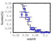
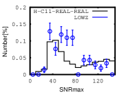
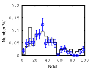
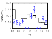
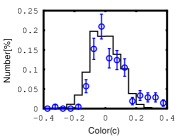
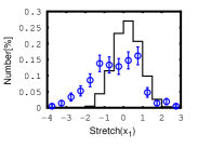
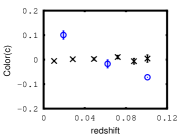
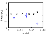
The quality of the simulations for the nearby, SDSS-II, and SNLS3-Megacam samples is illustrated with several data/MC comparisons in Figures 5 – LABEL:fig:REALDATA_SNLS.
|
|
|
|
Most aspects of the SDSS-II and SNLS3 MCs agree well with the observed data. The largest difference comes in fitted SALT-II color () and stretch () distributions, particularly for the nearby sample (e.g. Figure 5). As stated in Section 4.1.1, to simplify the implementation of the training tests we have chosen to use the same stretch and color parameter distributions for all SNe within a given training test, regardless of survey. Despite this simplification, our fitted MC mean color and stretch as a function of redshift agree reasonably well with their SDSS and SNLS data counterparts.
| mean | gen. range | |||
|---|---|---|---|---|
| Input Model = G10′ | ||||
| 0.0 | 1.0 | 0.7 | 2, 2 | |
| 0.0 | 0.07 | 0.1 | 0.3, 0.3 | |
| Input Model = H | ||||
| 0.5 | 1.0 | 0.7 | 2.5, 2.5 | |
| 0.0 | 0.07 | 0.1 | 0.3, 0.3 | |
Note. — The same distributions are used for all training data simulations with a given input model.
4.5. Determining Distances
The simulated test set is fit times, once by each realization of the trained model (see Figure 1). For each SN in the test set, the best-fitting scale (), stretch (), and color () parameters are determined by minimizing a based on the difference between the SN photometry and synthetic photometry of the model flux. To ensure good quality fits to the light curves, the following selection criteria are applied.
-
•
At least one observation before days.
-
•
At least one observation after days.
-
•
At least three filters with an observation that has a S/N above five.
-
•
At least five observations in the fitted epoch range to days.
The initial distance modulus for each test set SN is given by
| (10) |
where the effective -band magnitude is defined as and the global parameters , , and are determined by a fit of the entire test set using the SALT2mu program described in Marriner et al. (2011).
4.6. Redshift-dependent Bias Corrections
To obtain accurate cosmology parameters, flux-limited SN surveys must account for the impact of selection effects on distance modulus measurements. Typically this bias is determined by simulating SN Ia light curves from parameter distributions (color, stretch, ) consistent with the observed data, evaluating selection biases from these simulations, and correcting the initial distance moduli accordingly. Slight variations exist in the ways the simulated light curves are deployed and the biases are evaluated.
4.6.1 Bias Correction Method
In most previous analyses, bias corrections are calculated by analyzing the simulated bias data in a manner identical to the real data. In other words, the simulated light curves are generated and fit from the chosen SN Ia model, and subjected to any additional processing (i.e., global parameter fitting if using SALT) necessary to obtain distance measurements. The fitted distances are then compared with the underlying distances to obtain the recovered distance modulus bias as a function of redshift, and the real data are corrected accordingly. In terms of the fitted and simulated distances, the bias correction is
| (11) |
and the corrected distances are
| (12) |
This method has been used in Wood-Vasey et al. (2007) and Kessler et al. (2009a). In these works the corrections are usually described as “Malmquist bias” or “selection bias” corrections. However, by including light curve fitting as part of the process, this technique implicitly corrects for fitting biases as well as selection biases.
4.6.2 Bias Correction Simulation and Fitting
Following the schematic laid out in Figure 1, we generate our bias correction sets directly from the trained models; no lookup tables are created for these simulations. Each simulation’s intrinsic scatter function is taken from its trained model’s color dispersion applied as per the K13 prescription (Section 3.4.2).
Because the bias correction simulations should match the test set simulations as closely as possible, the same proportions of nearby, SDSS-II, and SNLS3 SNe are simulated with the same observing conditions as the test set. The number of SNe in the bias correction set is approximately the same as that of the test set.
Naively, one might expect that because we know the underlying ideal model parameter distributions, we can use those same distributions for bias correction simulations generated from our trained models. However, this is not the case. First, during the SALT-II model training, the stretch parameter mean and rms are rescaled from their initial distribution to a final distribution of and . Therefore, the trained model distribution will not be the same as the input model distribution. Second, we wish to approximate a data-based light curve analysis as closely as possible. When performing bias corrections on real SN Ia distances, the underlying stretch and color parameter distributions are unknown and must be backed out of the observed parameter distributions, which themselves suffer from redshift-related biases. Examples of this calculation can be found in D’Agostini (1995) and Kessler et al. (2009a).
To simplify our light curve analysis pipeline, we fit a high S/N realistic simulation with all trained model realizations and average the results to obtain an approximation of the underlying trained model stretch and color parameter distribution. In this same vein, the individual and values fitted by the trained models from the corresponding test set are used for the bias correction simulation.
Simulated bias correction SN light curves are fit with the trained model in a manner identical to the test set. Finally, SALT2mu is used to determine the best-fit , , and and to calculate distances for each set.
As an illustration, two sets of bias corrections are shown in Figure 6.
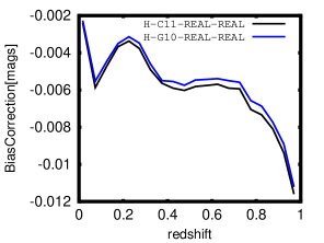
4.7. Cosmology
To obtain best-fit cosmology parameters, we fit the test set HD in a manner similar to the CDM fits described in Kessler et al. (2009a). We assume spatial flatness , but allow to differ from . SN distance moduli are combined with Baryon Acoustic Oscillation (BAO) and cosmic microwave background (CMB) constraints as described below.
For the BAO constraint, we use the quantity defined by Eisenstein et al. (2005),
| (13) |
and for the CMB we use the shift parameter
| (14) |
In both cases,
| (15) |
Rather than taking the best-fit and values from the data (e.g., Eisenstein et al., 2005; Komatsu et al., 2009), we determine and from our SN simulation cosmology parameters () and the experimentally determined redshifts and . To account for our much larger test sample, we scale the experimentally determined uncertainties by the equivalent number of G10 data sets (), such that
| (16) |
and
| (17) |
Tests have been performed to ensure that scaling the BAO and CMB uncertainties by the number of equivalent data sets produces the same result as averaging best-fit cosmology parameters from data sets.
Taken all together, the constraints on our best-fit cosmology are
| (18) |
and
| (19) |
In the absence of input SN data, these constraints yield the best-fit cosmology parameters and .
4.8. Final Distances and Best-fit Cosmology
Using the bias correction simulations and fits described previously (Section 4.6.1), bias corrections as a function of redshift are calculated using Equation 11 and applied to the recovered test set distances to obtain corrected distances . The corrected HD is fit to obtain final best-fit cosmology parameters and .
5. Training Test Evaluations
In this section we describe the quantities that will be used to evaluate the results of the training tests.
5.1. Quantities Derived From Training
To evaluate the performance of the training procedure, we begin by examining the training products themselves. The training process and products have been outlined in Figure 2 and described in Section 2. Color laws and color dispersions ) will be compared directly with those of the input model. The color dispersion residual is defined as
| (20) |
Similarly, the color law residual is defined as
| (21) |
By definition, the color law is defined for SNe with (e.g., Equation 1). Because the observed SN Ia color dispersion is 0.1, the quantity is the typical magnitude difference resulting from , and is the quantity we evaluate from here forward.
We also calculate residuals of the model components. First, the trained and input model surface fluxes are integrated over 1000-Å wide box filters centered on 3500 Å (), 4500 Å (), and 5500 Å (). The fractional flux difference is calculated for each filter independently, e.g., the -band residual is
| (22) |
For purposes of comparison, we take the H model “” surface to be the spectral time series with stretch and color both equal to zero.
5.2. Quantities Derived from Light Curve Fitting
For a given training test, it is interesting to compare the recovered , and distances with their input values. Various quantities may also be constructed from the distance moduli and . These actions are described in the following sections.
5.2.1 Hubble Scatter
Hubble scatter is defined as the dispersion on , the difference between the fitted distance modulus (e.g., Equation (10)) and the distance modulus calculated from the best-fit cosmological parameters.
This quantity is often used to characterize the quality of a light curve model. For a given SN Ia data set, the “best” model is the one that yields an HD with the smallest Hubble scatter. When calculated from HD of simulated data, the Hubble scatter may also be used as a test of the quality of the simulation. A high-quality simulation will yield Hubble scatter values similar to those observed with real data, typically from to for SALT-II light curve fits.
For our cosmology results, we calculate Hubble scatter from the uncorrected SN distances as described above. However, when evaluating regularization schemes (Section 6.2.1) we simplify the calculation of this quantity slightly by computing the dispersion of .
5.2.2 Hubble Bias
Hubble bias is the difference between the recovered HD and the true HD as a function of redshift. In this work, we use simulated data to measure Hubble bias stemming from SALT-II light curve analyses. In other words, our Hubble bias indicates the accuracy of a measured SN Ia distance modulus in a particular redshift bin. In the limit of a “perfect training,”666A training performed with an infinitely large, high cadence, and high S/N training set we expect that the Hubble bias should go to zero for all redshifts. In Section 6.1 we check that this is indeed the case. We also measure Hubble bias for models trained from simulations designed to mimic the G10 training set in composition, S/N, and cadence. These measurements may be used as estimates of the systematic uncertainty as a function of redshift for HD made with the G10 SALT-II model.
For a single test supernova SNi, we calculate the average fitted distance modulus over all training realizations as
| (23) |
and define the Hubble bias as the difference between the average distance modulus (23) and the actual distance modulus
| (24) |
5.2.3 Training Model Scatter
This quantity, defined below, quantifies the reproducibility of an individual SN’s measured distance modulus as a function of redshift. In this sense, training model scatter is a measure of the uncertainty in the trained model due to the training set sample size. In the limit of a perfect training, the training model scatter should approach zero in all redshift bins. Our training model scatter calculations will be used to evaluate the SALT-II model statistical uncertainty estimations described in G10.
For a single test SNi, we define the training model scatter as the dispersion of the fitted distance moduli (where runs over training realizations 1 to ) about the mean fitted distance modulus :
| (25) |
6. Results
6.1. Test Case 1: Ideal Training
We are working under the hypothesis that given enough input data, the SALT-II training process will produce an accurate copy of the input model, and that light curve fits made with such a trained model will recover input cosmology to high accuracy. For this work, we define an “IDEAL” training as one in which a comprehensive, high-quality training set is used as input. In this section, we describe the test set used for these trainings and the results of our training tests.
6.1.1 Ideal Training Set
Our IDEAL trainings are based on the H and G10′ input models paired with no intrinsic scatter (i.e., scatter model NONE). We generated 10 independent realizations of the IDEAL training set, each with its own set of independent random seeds. These training sets consist of two samples: 110 simulated nearby SNe drawn from a flat redshift distribution spanning , and 110 simulated SDSS SNe drawn from a flat redshift distribution spanning . For both samples, the photometry is of high quality, with two-day observer-frame cadence and S/N at peak or band regardless of redshift. Spectra are of similarly high quality. Seven spectra are generated for each simulated supernova, with the first observation date randomly chosen between rest frame epochs 14 and 4 days, and the remaining spectra spaced every 10 rest-frame days thereafter. This selection mechanism results in a uniform distribution in phase of the observations of supernova spectra. All spectra span rest frame wavelengths 2000 to 9200 Å, and have S/N defined on a bin size of 100 Å.
Given the high-quality training sets the training configuration is adjusted accordingly. Bands in the ultraviolet region are not de-weighted. Because our training set spectra have no calibration errors, we turn off photometry-based spectral rescaling. Finally, although we implement nominal regularization, the high sampling of the input data makes regularization irrelevant.
6.1.2 Ideal Test Set
Once training is complete, the new IDEAL models are evaluated by using them to fit large, similarly high-quality test sets. As with the training sets, our test sets are generated from either the H or the G10′ input model paired with no intrinsic scatter (i.e., scatter model NONE). These test sets (which we also call IDEAL) consist of 4000 SDSS and 4000 SNLS SNe. The relevant spectroscopic selection efficiencies have been applied to the data set, but the exposure times of the simulations have been adjusted to give photometric data with S/N in the -band at peak. Light curve fits of the SDSS test sample are performed with photometry; fits of the SNLS test sample are performed with photometry. The fitted light curve parameters are then used to determine the global best-fit , and values, and initial SN distances , as described earlier in Section 4.7. Finally, bias corrections are applied to derive the corrected SN distances , and best-fit cosmology parameters and are obtained.
6.1.3 Trained Model Residuals
Because we have tailor-made our fiducial G10′ SN Ia model to match SALT-II training capabilities (see Section 3.2), synchronized our simulation software with our training software, and trained with extensive, high S/N training sets, we expect that the resulting G10′-NONE-IDEAL-IDEAL trained models will match the input model well in all bands. Our input H model has no input from or connection to the SALT-II model, so we do not expect H-NONE-IDEAL-IDEAL trained surfaces to reach the same level of agreement.
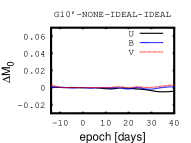
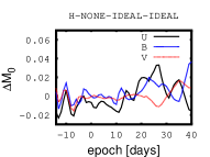
Plots of surface residuals bear out these expectations. Figure 7 shows the mean integrated flux residuals and mean color law residuals for our ideal training tests.
 |
 |
 |
 |
The G10′ integrated flux residuals are smaller than in flux in all bands except (which agrees to in flux), indicating excellent agreement between the input and trained model surfaces. Near peak luminosity, the H model values are similarly small ( in flux), but increase to in flux at early and late epochs, particularly in the bluest wavelength ranges. We attribute this difference to the inability of the SALT-II training code to exactly reproduce the stretch features of the H model. Color law residuals are small for both models, no larger than 0.0005 mags for .
6.1.4 Cosmology Residuals
| Training Options | aaThe simulated value of is 0.11. As described in Section 2.5 and Appendix A, the expected values of are model-dependent, and typically . | bbThe simulated value of is 3.2. | |||
|---|---|---|---|---|---|
| G10′-NONE-IDEAL-IDEAL | 0.000 | 0.080 | |||
| H-NONE-IDEAL-IDEAL | 0.000 | 0.163 |
Note. — Mean cosmology parameters recovered by ideally trained models on ideal data sets. Model naming conventions are described in Table 2. All errors are errors in the mean.
Each of the 10 trained model realizations was used to fit a single ideal set of 8000 test SNe light curves. SALT2mu was applied to the resulting light curve parameters to obtain 10 sets of best-fit model values , and , and 10 sets of distance moduli to use for cosmology fits. Assuming a flat CDM cosmology, a chi-squared minimization was used to determine and for each realization. The mean recovered values of , , and are shown in Table 5.
As described in Section 2.5 and Appendix A, the rescaling of the parameter that occurs during SALT-II model training changes the value of from its input value of to an expected value closer to . Both trainings recover mean values somewhat smaller than the expected value: 0.094 for the G10′ model and 0.090 for the H model. A discrepancy in is expected for the H model, since the stretch function used to create the SED width–magnitude relation cannot be exactly recreated with the SALT-II linear combination of surfaces. The two training tests recovered and with high precision and within of the input values. For our ideal test sets, the bias is flat as a function of redshift: both the raw and the bias-corrected are recovered within the limit of 0.005.
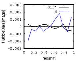
Figure 8 shows the Hubble bias as a function of redshift for the H and G10′ trainings. The average distance modulus differs from the true distance modulus by less than 0.003 mags in all redshift bins. As with the surface residuals , the G10′ input model has smaller Hubble bias than the H input model. However, in either case, the bias is small compared to the overall precision of the measurements.
6.1.5 Ideal Training Test Conclusions
With the exception of slightly low recovered values, training the SALT-II model with a complete, well-sampled, high quality set of data results in the recovery of the input model with high accuracy. For both models, the mean SED broadband-integrated flux is recovered to better than in all bands for phases between 10 and 10 days of the -band maximum. At late times, the maximum flux difference seen for the H model is , and for the G10′ model, only .
When applied to an ideal set of test data, the ideally trained models yield Hubble biases smaller than 0.002 mags at all redshifts and recover with high accuracy. After applying bias corrections, the final bias is for the H model and for the G10′ model.
6.2. Test Case 2: Realistic Training
Having established that the training procedure is able to reproduce the input model under ideal conditions (i.e., full phase-space coverage by the training set, no intrinsic scatter) we proceed to test SALT-II training with more realistic training and test data. We define a “REAL” training as one in which the simulated training and test set SN Ia redshift distributions, cadences, and S/N closely match the SALT-II G10 training and test set data. We examine the impact of regularization on trainings with realistic S/N and cadence but without intrinsic scatter, and select the best regularization settings to use for our realistic training tests. We then describe the results of our full realistic training tests, including trained model residuals, Hubble scatter, and cosmology results.
6.2.1 Regularization Tests
As described in Section 2, “regularization” refers to the addition of extra terms to the , with the goal of reducing the amount of artificial structure on small wavelength scales trained into regions of the best-fit model where input data is sparse. Ringing in the best-fit model adds extra scatter to light curve fits, thereby reducing the precision with which distances and cosmology parameters can be measured. On the other hand, the addition of regularization terms can systematically bias the best-fit model. Therefore, uncertainties due to regularization must be measured and accounted for in the distance modulus error budget.
The forms of regularization used in this work are described in Section 2.3. The overall strength of each term is determined by an arbitrary weight. G10 evaluated the change in mean distance modulus as a function of redshift for two different regularization weights. They found the change to be small, less than or equal to 0.005 mags for redshifts below 1. Using our simulation techniques we reevaluate the impact of regularization on bias.
Methods
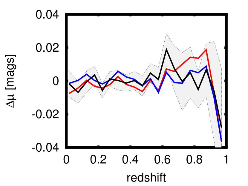
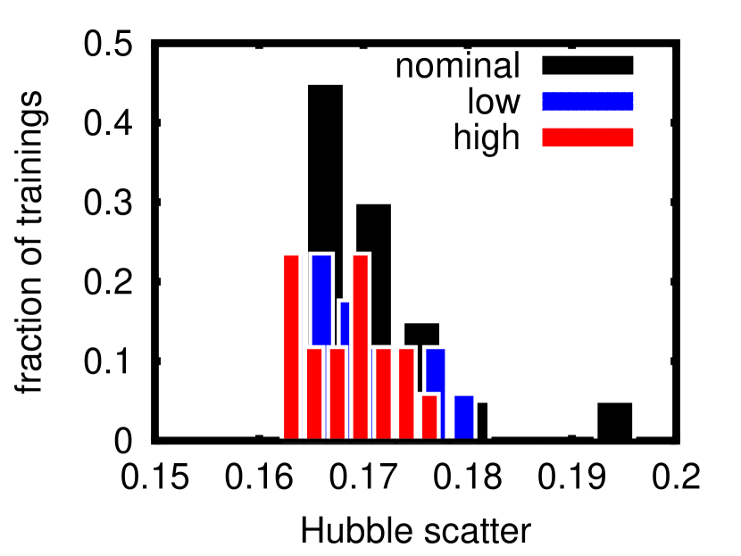
We define nominal regularization weights as those used in the G10 training, i.e., 10 for the gradient term and 1000 for the dyadic term. H-C11-REAL-REAL trainings have been run for three sets of regularization weights: “nominal,” “high” (nominal), and “low” (nominal). The same regularization terms and weights are applied to both and . To determine the optimal regularization, we compare average Hubble biases and Hubble scatter (see Section 5.2) for the three trainings. As mentioned previously, these Hubble scatter results have been calculated with simulated values of alpha and beta (0.11 and 3.2, respectively), rather than with the SALT2mu fitted values which change from realization to realization. We have checked that this simplification does not alter our conclusions. Results of these comparisons are shown in Figure 9 and Table 6.
| Training Options | |||||
|---|---|---|---|---|---|
| NOMINAL | 0.125 | 20 | |||
| 0.124 | 17 | ||||
| 0.123 | 17 |
Note. — Mean cosmology parameters recovered by realistically trained models on realistic data sets. All errors are errors in the mean.
Results
Minimal differences are observed between , nominal-regularization, and Hubble biases (e.g., top panel of Figure 9). Recovered are equivalent to within 0.005 mags for most redshifts, with the only small discrepancy (1-) seen in the redshift region . This finding is consistent with the regularization tests described in G10. As shown in the lower panel of Figure 9, regularization has little effect on Hubble scatter. Finally, and nominal regularizations recover entirely consistent results, consistent with each other and consistent with the input value at the level. The regularization yields a less consistent value of , differing from the input at .
Based on the results, we choose nominal regularization as the best training choice. Nominal regularization produces the same Hubble bias and Hubble scatter as low regularization, and results in a slightly more consistent recovery of .
6.2.2 Simulations and Training Configuration
Our realistic trainings incorporate intrinsic scatter, described by the scatter models COH, G10, and C11, into both the training sets and the test sets. For the six possible combinations of input model and scatter model (e.g., Table 2), 20 independent training set realizations have been generated, each with its own set of random seeds. Recall that our REAL training sets consist of 220 simulated SNe with redshift distributions, cadences and S/N pattered after the low-redshift sample and the SNLS3 sample. Details of the light curve and spectral simulations are presented in Sections 4.4 and 4.2.1.
Training configurations are similar to those used in the G10 paper. We use nominal regularization (see Section 6.2.1) and a spectral recalibration step size of 800 Å corresponding to the typical width of a broadband filter. We do not de-weight bands in the ultraviolet region.
As with the IDEAL training tests, we evaluate our REAL trained models by using them to fit large test sets of simulated SN Ia light curves generated from the same input models and parameter distributions as the training sets. We continue to fit IDEAL test sets (as described in Section 6.1.2), but add to these fits and analyses of REAL test sets, which include not only realistic spectroscopic selection efficiencies, but also realistic photo-statistics.
6.2.3 Model Residuals
Analogous to our presentation of the ideal training tests, we start by examining residuals of the trained surfaces and color laws with respect to the input models. We compare the observed spread in (, Equation 25) with the analytic estimates made in G10. Finally, we examine how well input cosmology parameters are recovered and determine the recovered distance modulus biases as a function of redshift.
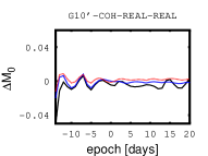
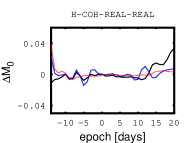
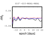
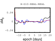
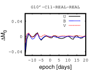
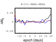
In general, all six trainings recover the surface reasonably well. Figure 10 shows light curve residuals as a function of phase for the six main realistic trainings. The largest residuals, up to a difference in flux, are seen at early and later phases. All six models have residuals at days: the G10′ input models in , and the H input models in . At later phases, days, all six models agree well in . Two of the G10′ models, G10′-COH-REAL-REAL and G10′-C11-REAL-REAL, also agree well in , whereas the other four input models have .
 |
 |
 |
 |
 |
 |
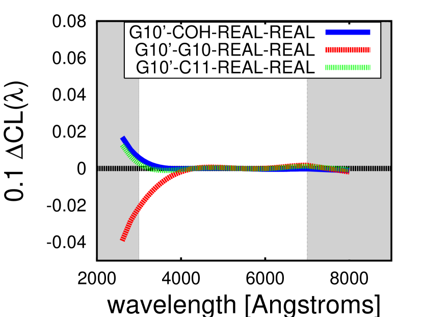
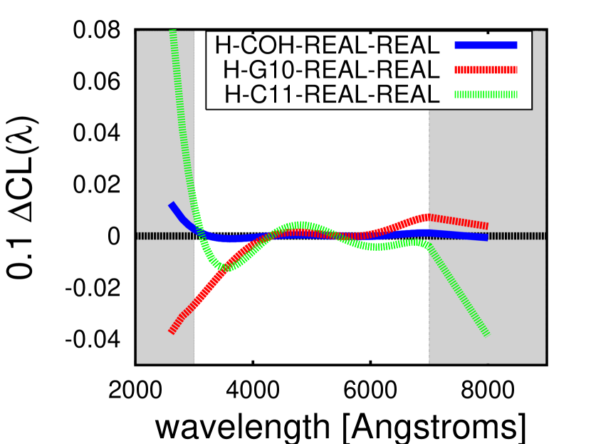
Color law residuals are not uniformly well recovered. As seen in Figure 11, the coherent scatter trainings return color laws in excellent agreement with the input model. However, the other scatter models show deviations from the input at wavelengths below 3500 Å and, for the C11 scatter model in particular, above 7000 Å. Overall, the shapes of the color law residuals are similar for all trainings using the C11 scatter model regardless of the input model chosen: at the smallest wavelengths, the recovered color laws have 15%–25% more extinction than the input color laws. The G10′-G10-REAL-REAL color law residual has a similar wavelength dependence as the G10′-C11-REAL-REAL color law residual, whereas the H-G10-REAL-REAL color law residual is quite different in shape from the H-C11-REAL-REAL color law residual; of the four trainings shown in Figure 11, H-G10-REAL-REAL alone results in a trained model with smaller blue extinction than the input model.
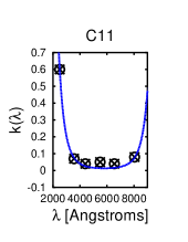
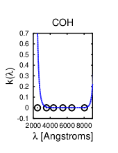
Finally, we can compare the recovered broadband color dispersions with the input models. The input COH scatter model does not change SN colors (i.e., ). For the input C11 scatter model, the diagonals of the reduced correlation matrix are used as a proxy for its dispersion as a function of wavelength.777See Table 4 of K13. Analogous quantities for the input G10 scatter model are the G10 values at 2500 Å and at central wavelengths. The recovered dispersions are the trained functions. Figure 12 shows the input and recovered dispersions as a function of wavelength for our three realistic intrinsic scatter models C11, COH, and G10. The choice of input model (G10′ or H) makes very little difference to the recovered ; therefore only H-based training results are displayed in Figure 12.
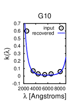
The input broadband dispersion is recovered reasonably well at all wavelengths for the C11 scatter models. The recovered G10 and COH dispersions match the input dispersions above 3500 Å but diverge in the near-UV. The divergences at the extreme blue and red regions are from inadequate spectral coverage and regularization effects. Although the divergences in G10 and COH are significant, the wavelength regions of the discrepancies are so blue (and red, in the case of COH) that their relevance to SN Ia light curve fits should be minimal.
 |
 |
 |
6.2.4 Statistical Uncertainty Estimates
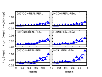
Using multiple training set realizations, we have been able to directly measure the scatter in SN Ia distance measurements as a function of redshift due to training statistics. In Figure 13, we compare our results with estimates calculated by G10. Our distance scatter measurements include both the wavelength dispersion uncertainty and training statistical uncertainty; thus, we have combined the analogous components of the G10 estimates. Because cosmology depends only on relative distances, we consider only the relative scatter .
Intrinsic scatter model and redshift are the key determinants of . In general, the COH scatter model has the smallest and C11 has the largest . For all input scatter models is flat for redshifts below 0.6, and ranges from 0.00 to 0.02 mags. At higher redshifts, increases up to a maximum of 0.03 to 0.11 mags at , with the G10′-COH-REAL-REAL model having the lowest scatter and the H-C11-REAL-REAL model having the most scatter. The SALT-II estimates agree well with our results for all intrinsic scatter models.
6.2.5 Hubble Bias and Cosmology
Fits of realistically trained models on realistic test data yield the mean recovered values of , , and shown in the first six rows of Table 7.
| Training Options | aaThe simulated value of is 0.11. As described in Section 2.5 and Appendix A, the expected values of are model-dependent, and typically . | bbThe simulated value of is 3.2. | |||
|---|---|---|---|---|---|
| G10′-COH-REAL-REAL | 0.133 | 13 | |||
| H-COH-REAL-REAL | 0.131 | 12 | |||
| G10′-G10-REAL-REAL | 0.125 | 16 | |||
| H-G10-REAL-REAL | 0.119 | 16 | |||
| G10′-C11-REAL-REAL | 0.124 | 18 | |||
| H-C11-REAL-REAL | 0.125 | 20 |
Note. — Mean cosmology parameters recovered by realistically trained models on realistic data sets. Model naming conventions are described in Table 2. All errors are errors in the mean.
As described in Appendix A and shown in Table 9, the expected values of are roughly smaller than the input value of 0.11, and vary with input model. Taking this effect into account, our recovered parameters agree reasonably well with expectations.
Only one of our six training tests — G10′-COH-REAL-REAL — recovers consistent () with the input value of 3.2. Because our realistic test data suffers from selection effects, and because is fit prior to applying bias corrections, some decrease in is to be expected. However, our values vary with input scatter model. With an average , the COH intrinsic scatter trainings come closest to the input value. G10 intrinsic scatter tests are the next closest, with an average of , whereas the trainings with C11 color scatter have the most discrepant values with average . As we will discuss further in Section 7.2, our finding is consistent with other results, including K13 and Chotard et al. (2011).
Also shown in Table 7 are our recovered values. After corrections, all recovered values are slightly smaller than the input value of . Four of the six training tests recover consistent with the input at the level; the two that do not are G10′-COH-REAL-REAL, which recovers for a 2.0- difference, and G10′-C11-REAL-REAL, which recovers for a 2.4- difference.
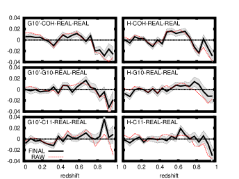
Figure 14 shows distance bias as a function of redshift for each of our training configurations. The distance bias has been binned in redshift steps of . Both the final bias and the raw bias (before applying bias corrections) are shown. As expected, bias corrections reduce , with the impact of the reductions being most significant in the low- and high-redshift regions ( and ). The exception is the training G10′-C11-REAL-REAL, for which bias corrections make the distance bias worse at redshifts larger than 0.8.
7. Discussion
In the following sections, we will discuss some of the implications of our residuals and biases, examine procedures for redshift-bias correction, and remark on implications for optical SN Ia cosmology and future model training.
7.1. Trained Model Biases
Adding realistic intrinsic scatter to the simulated SALT-II training set yields biased models. In general, these biases are small and are concentrated in the UV ( Å). As seen in Figure 10, all flux residuals exhibit oscillations in all bands at early and late epochs ( days, days). G10′ flux residuals oscillate slightly at all epochs. In addition, G10′ flux residuals decrease to in at epochs less than 10 days, whereas the H residuals increase to at epochs greater than 10 days. Trained color laws and color dispersions also show biases in the UV. Three of the four realistic scatter model trainings have biased color laws at wavelengths bluer than 4000 Å (Figure 11), and the G10 scatter model training tests underestimate broadband dispersion at wavelengths bluer than 3000 Å (Figure 12).
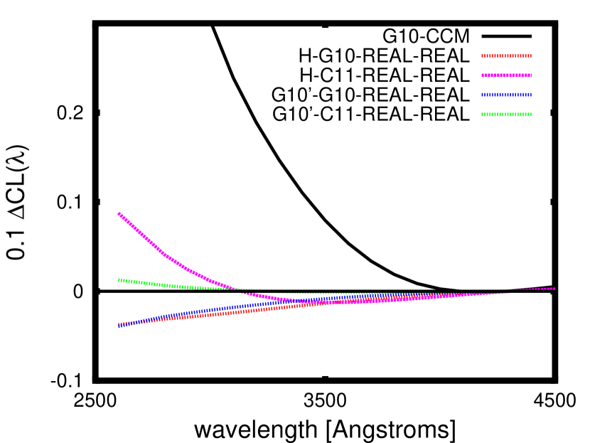
The colored lines in Figure 15, a magnified version of the low-wavelength regions of Figure 11, present the difference between the recovered and the input color laws for the four realistic-intrinsic-scatter models. In the same figure, the solid black line shows the difference between the G10 model color law and the CCM extinction law. The observed color law biases from our training tests are less than 0.03 mag in the wavelength region most relevant for light curve fitting ( Å), compared with a G10–CCM difference of mag in the same wavelength region.
Based on this result, we conclude that the training process itself is not responsible for the observed difference between G10 and CCM color laws. However, we have not eliminated the possibility that the SN Ia training set is a source of this difference: as currently configured, our simulated training set does not include systematic calibration offsets, nor have we attempted to simulate differences in SN Ia populations at low and high redshifts.
Both C11 scatter model training tests exhibit positive biases below Å. This trend is in the same direction as the observations of Maguire et al. (2012), who found that the G10 color law overcorrected UV spectral fluxes in comparison to the CCM color law. However, the size and wavelength region of our bias is smaller and bluer than the effect Maguire et al. (2012) describe.
7.2. Biased Color and Biased
Biases in the model affect its ability to correctly fit for the color parameter in redshift regimes where rest-frame UV and data are important. In turn, incorrectly fitted parameters as a function of redshift yield recovered values that differ significantly from the input values. All of our recovered values are smaller than the input value of . Training tests based on COH intrinsic scatter models recover , a value within 2- of the input On the other hand, training tests performed with G10 intrinsic scatter models result in values of , and those based on C11 scatter models yield , both significantly lower than the input value.
A similar effect has been described by K13, who reported scatter-model-dependent recovered values when fitting simulated light curves with fixed intrinsic scatter . K13 added realistic intrinsic scatter to SN Ia light curves simulated from the G10 , , and CL. The resulting light curves were fit with the G10 model. As we do here, K13 evaluated three types of scatter: coherent, G10, and C11888K13 used two C11 variants. Their “C11_0” is the one we have used in this work.. They recovered values equal to or smaller than the input value: for coherent scatter , for G10 scatter , and for C11 scatter . In other words, K13 found to be recovered correctly for those simulations generated either with COH or with the same scatter model as the model used to fit the data, and to be recovered as significantly smaller for those simulations generated with a different scatter model than the model used to fit the data.
A key difference between our work and K13 is that we retrain the SALT-II model. Thus our test set light curves are always simulated with a model different from the one used to fit them. In this sense, our results — in which we find both G10 and C11 scatter model to be significantly lower than their input values — are entirely consistent with the results of K13. As discussed by K09 and G10, color law biases can result in redshift-dependent values of even if the underlying value of is constant. By allowing our values to float with redshift, this effect appears in our test samples. We divide our TEST SNe Ia into redshift bins of width=0.1 and fit each bin individually for . The resulting values of , along with the values observed by G10 from real SNLS3 data, are shown in Figure 16. Training tests with no added intrinsic scatter show minimal (no) change in when applied to ideal (realistic) test samples. When intrinsic scatter is added, both ideal and realistic training tests have identical / until a redshift of 0.65 when Malmquist bias causes the realistic test sample / to decrease more rapidly. With the exception of one redshift bin, the mean obtained from our simulated samples is in good agreement with G10 SNLS3 results (see Figure 17, Guy et al., 2010).
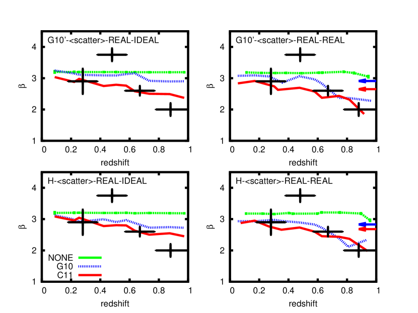
Because the recovered value of is sensitive to small biases in the color law and broadband dispersion, the effects of training on the recovered value of should be taken into account to determine the underlying value. G10 recovered ; our results suggest the bias-corrected value of is 3.65–3.82.
Furthermore, if light curve analysis produces the correct cosmology parameters, biases in the recovered beta values are somewhat irrelevant. In terms of our ability to recover cosmological parameters, the significance of color law biases is small. As shown in Table 7, after simulated bias corrections are applied, the best-fit values are underestimated by 0.01–0.02 depending on the choice of input scatter model.
| Training Options | |||||
|---|---|---|---|---|---|
| G10′-COH-REAL-REAL | 0.133 | 17 | |||
| H-COH-REAL-REAL | 0.131 | 19 | |||
| G10′-G10-REAL-REAL | 0.125 | 16 | |||
| H-G10-REAL-REAL | 0.119 | 16 | |||
| G10′-C11-REAL-REAL | 0.124 | 18 | |||
| H-C11-REAL-REAL | 0.125 | 20 |
Note. — Mean cosmology parameters recovered by realistically trained models on realistic data sets. Model naming conventions are described in Table 2. All errors are errors in the mean.
As shown in Table 8, generating the bias correction simulations from the input model rather than the trained model causes the observed biases to disappear. The sole exception is the H-COH-REAL-REAL model, whose bias becomes worse rather than better. However, the COH scatter model is clearly unrealistic. Recovering the correct values of for the more realistic G10 and C11 scatter models validates our bias correction procedure, and points to differences between the trained and input model as being the source of the observed bias in . In other words, if we knew the true underlying SN Ia model and were able to generate bias correction simulations from that model directly, our bias correction technique would correctly compensate for redshift-dependent biases induced by the training. Instead, we generate bias correction simulations from our imperfect trained model. These corrections are not quite right, resulting in a slightly biased value.
7.3. SNLS3 Bias Corrections
The SNLS3 cosmology analysis (Sullivan et al., 2011) uses a bias correction technique which is slightly different from the TOTAL method used in this work. As described by Perrett et al. (2010), the SNLS3 analysis inserts simulated SN light curves directly into SNLS survey search images and runs them through the discovery pipeline in the same manner as their real data. The simulations are configured such that each simulated SN Ia’s actual (including both stretch and intrinsic dispersion variations) are known a priori. For the set of detected real SNe Ia, the applied selection bias correction arises from the recovered as a function of redshift. The simulated light curves are never fit.
We performed our training tests using an approximation of this bias correction method (described in Appendix B). For each scatter model tested, recovered values are indistinguishable from those determined with the TOTAL correction, and the average bias is consistent with our nominal result.
7.4. Impact of Scatter Models on HD Biases and Cosmology
After omitting results from the unphysical COH model, we see no strong differences in the bias as a function of intrinsic scatter model. The bias obtained from our remaining four realistic scatter-model trainings are indistinguishable within the uncertainty. For the C11 training tests alone, the average bias is , which is fully consistent with the “Nearby + SDSS-II + SNLS3” C11_0 Malmquist-corrected -bias of reported by K13. The average bias of our G10 training tests is , smaller than the observed by K13. As stated earlier, K13 did not retrain the SALT-II model for their tests. The training process introduces biases in the trained model which result in slight biases in , even after application of the bias corrections. The results presented here supercede the results in K13.
Combining the results from the remaining four realistic trainings, we find an average bias of .
7.5. Using these Results to Improve Constraints on Dark Energy
We have used a series of MC samples to train the SALT-II model and measure HD biases as a function of redshift. Our MC samples were specifically designed to match the SNLS3 SN Ia cosmology sample (e.g., Conley et al., 2011).
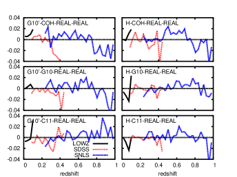
HD bias as a function of survey is shown in Figure 17. Because our HD bias measurements incorporate uncertainties due to the SN Ia model, intrinsic scatter, regularization, global parameter values (e.g., ), and bias corrections in a self-consistent way, these survey-dependent HD bias measurements are used by Betoule et al. (2014) (B14) to update SN Ia model-related systematic error estimates from the most recent SNLS3 cosmology analysis (Sullivan et al., 2011).
While the B14 training and cosmology samples are not identical to the ones used here — the training sample includes SDSS photometry and the cosmology sample includes SN Ia light curves from the full 3-year SDSS survey — they are similar enough to enable the transfer of HD bias results (e.g., Figure 17). Our SDSS-II simulation parameters (e.g., cadence, imaging noise, and selection function) are drawn from the full three-year sample and the addition of SDSS-II light curves to the training set does not significantly alter the trained model. Note that different training samples and/or surveys will produce different biases in the cosmology, thus this calculation must be adapted to each specific analysis.
8. Conclusions
We have used simulated SN Ia samples to determine that SALT-II model training, fits, and bias correction of the SNLS3 cosmology sample published in Sullivan et al. (2011), and introduce a redshift-dependent HD bias, resulting in a bias on . Here, we have excluded the COH scatter model results, as this scatter model is clearly unphysical. The uncertainty on is given by the rms of the remaining four input and scatter model results. In order to perform these tests, we have upgraded the SN analysis software package SNANA to enable spectrum simulations incorporating realistic photo-statistics, galaxy contamination, and intrinsic scatter.
When the SALT-II model is trained on an SN Ia spectral time series with no intrinsic scatter and a high-quality MC training set, we are able to recover the input model components , , and CL, and obtain an HD with no biases. When the training set is made more realistic via the addition of intrinsic scatter to the input model and a reduction in the training set size and S/Ns, we predict a bias that agrees well with the profile reported in G10, and conclude that there is no evidence for a redshift-dependent value of . We have also verified that the estimates of G10 accurately predict the statistical uncertainty in SN Ia distances due to the training sample size.
We confirm the findings of K13 that the recovered value of depends on the intrinsic scatter model assumed. By adding the training process, we extend the work of K13 to discover that training biases both G10 and C11 results: both intrinsic scatter models result in smaller recovered values and slightly biased, consistent values. Our G10 training tests yield a bias () of ; our C11 training tests produce a bias of .
Differences between the trained model and the underlying model alter the measurement of individual SN Ia color parameters as a function of redshift, and cause the recovered color correction parameter to be systematically underestimated. The extent to which the recovered deviates from the input depends on the form of the intrinsic scatter. Using G10 scatter results in biases of ; using C11 scatter results in biases of . The underlying value of requires a bias correction, and this correction depends on the nature of intrinsic variations. G10 recovered ; our results suggest that the bias-corrected value of is 3.65–3.82.
Although the scatter models used in this work have been thoroughly tested (K13) and found to reproduce key photometric observables such as photometric redshift residuals, Hubble scatter, and color dispersion, they are solely dependent on wavelength, and as such are somewhat unrealistic. Intrinsic scatter most likely results from a combination of effects, including metallicity, viewing angle, and progenitor properties. Thus, in addition to the wavelength dependence assumed in our models, the intrinsic scatter may also depend on phase, stretch, color, and redshift. An improved understanding of the origins and nature of intrinsic scatter will be important for reducing systematic uncertainties in future SN Ia distance measurements.
The procedure we have used in this work provides a recipe for evaluating systematic errors due to light curve analysis. Although our HD bias measurements are model and survey specific, our procedure is general and may be adapted to test other SN Ia models and data samples. Given a training set and a cosmology set of SNe Ia, a corresponding training sample simulation can be used to train a light curve model. Using the trained model, distances may be fitted from a corresponding simulated cosmology sample. Finally, HD and biases can be determined. These biases may then be incorporated into the systematic error budget of the data sample.
The HD biases measured in this work have been used to evaluate model-related systematic uncertainties in a joint SDSS+SNLS cosmology analysis reported in B14.
9. Acknowledgements
J.F. and R.K. are grateful for the support of National Science Foundation grant 1009457, a grant from “France and Chicago Collaborating in the Sciences” (FACCTS), and support from the Kavli Institute for Cosmological Physics at the University of Chicago.
This work was completed in part with resources provided by the University of Chicago Research Computing Center.
M.S. is supported by the Department of Energy grant DE-SC-0009890.
Appendix A Expected alpha determination
Mixing between the input and parameters during the training process is not unexpected, and will lead to predictable changes in the recovered model parameter.
The training process separates color from width by assuming that the peak color will be zero for all SNe with , regardless of value. If the input training set shows some variation in color with , such that the observed color follows the form , the width-varying part of the color will be incorporated into the SALT-II model term as follows:
| (26) |
where , , , and are the -correction, distance modulus, width, and color of a specific SN Ia, and , , and are global SN Ia parameters.
By linearly fitting peak color as a function of for each of our input models, and normalizing this slope with respect to the base G10 model such that , we can measure the slope and predict the expected alpha value :
| (27) |
We have used this technique to calculate expected values for as a function of input model; these values are shown in Table 9.
| Training Options | |
|---|---|
| GP-NONE | 0.100 |
| H-NONE | 0.102 |
| GP-G10 | 0.079 |
| H-G10 | 0.106 |
| GP-C11 | 0.099 |
| H-C11 | 0.100 |
Appendix B Redshift-dependent bias corrections
As an alternative to the TOTAL technique adopted earlier in this work, we consider the “MALM” bias correction technique used by the SNLS3 cosmology analysis. As described by Perrett et al. (2010), simulated SNe light curves are generated independently from the SNLS3 fitting models (SALT-II and SIFTO), inserted directly into search images, and run through the discovery pipeline in the same manner as the actual data. The simulations are configured such that each simulated SN Ia’s actual (including both stretch and intrinsic dispersion variations) is known a priori. For the set of detected SNe Ia, the applied selection bias correction comes from the recovered as a function of redshift. The simulated data are never fit.
Although we are unable to implement this technique in a fit-independent manner, we approximate it here by simulating a realistic full SN Ia sample (i.e., no efficiency cuts are applied), fitting the sample with minimum selection cuts, and comparing the distance moduli thus derived to the distance moduli from a “detected” sub-sample (i.e., those passing our efficiency cuts). Within this framework, we define the MALM bias as:
| (28) |
| Training Options | (TOTAL) | (MALM) | ||||
|---|---|---|---|---|---|---|
| G10′-COH-REAL-REAL | 0.133 | 13 | ||||
| H-COH-REAL-REAL | 0.131 | 12 | ||||
| G10′-G10-REAL-REAL | 0.125 | 16 | ||||
| H-G10-REAL-REAL | 0.119 | 16 | ||||
| G10′-C11-REAL-REAL | 0.124 | 18 | ||||
| H-C11-REAL-REAL | 0.125 | 20 |
Note. — Mean cosmology parameters recovered by realistically trained models on realistic data sets. Model naming conventions are described in Table 2. All errors are errors in the mean.
References
- Bailey et al. (2009) Bailey, S., et al. 2009, A&A, 500, L17
- Barone-Nugent et al. (2012) Barone-Nugent, R. L., et al. 2012, MNRAS, 425, 1007
- Bessell (1990) Bessell, M. S. 1990, PASP, 102, 1181
- Betoule et al. (2014) Betoule, M., Kessler, R., Guy, J., Mosher, J., et al. 2014, A&A, 568, 32
- Betoule et al. (2013) Betoule, M., et al. 2013, A&A, 552, A124
- Calzetti et al. (1994) Calzetti, D., Kinney, A. L., & Storchi-Bergmann, T. 1994, ApJ, 429, 582
- Chotard et al. (2011) Chotard, N., et al. 2011, A&A, 529, L4
- Conley et al. (2008) Conley, A., et al. 2008, ApJ, 681, 482
- Conley et al. (2011) —. 2011, ApJS, 192, 1
- D’Agostini (1995) D’Agostini, G. 1995, Nuclear Instruments and Methods in Physics Research A, 362, 487
- Doi et al. (2010) Doi, M., et al. 2010, AJ, 139, 1628
- Eisenstein et al. (2005) Eisenstein, D. J., et al. 2005, ApJ, 633, 560
- Foley & Kasen (2011) Foley, R. J., & Kasen, D. 2011, ApJ, 729, 55
- Frieman et al. (2008) Frieman, J. A., et al. 2008, AJ, 135, 338
- Fukugita et al. (1996) Fukugita, M., Ichikawa, T., Gunn, J. E., Doi, M., Shimasaku, K., & Schneider, D. P. 1996, AJ, 111, 1748
- Gunn et al. (1998) Gunn, J. E., et al. 1998, AJ, 116, 3040
- Gunn et al. (2006) —. 2006, AJ, 131, 2332
- Guy et al. (2007) Guy, J., et al. 2007, A&A, 466, 11
- Guy et al. (2010) —. 2010, A&A, 523, A7+
- Hamuy et al. (1996) Hamuy, M., et al. 1996, AJ, 112, 2408
- Hicken et al. (2009) Hicken, M., et al. 2009, ApJ, 700, 331
- Holtzman et al. (2008) Holtzman, J. A., et al. 2008, AJ, 136, 2306
- Hsiao et al. (2007) Hsiao, E. Y., Conley, A., Howell, D. A., Sullivan, M., Pritchet, C. J., Carlberg, R. G., Nugent, P. E., & Phillips, M. M. 2007, ApJ, 663, 1187
- Jha et al. (2007) Jha, S., Riess, A. G., & Kirshner, R. P. 2007, ApJ, 659, 122
- Jha et al. (2006) Jha, S., et al. 2006, AJ, 131, 527
- Kattner et al. (2012) Kattner, S., et al. 2012, PASP, 124, 114
- Kessler et al. (2009a) Kessler, R., et al. 2009a, ApJS, 185, 32
- Kessler et al. (2009b) —. 2009b, PASP, 121, 1028
- Kessler et al. (2013) —. 2013, ApJ, 764, 48
- Kinney et al. (1996) Kinney, A. L., Calzetti, D., Bohlin, R. C., McQuade, K., Storchi-Bergmann, T., & Schmitt, H. R. 1996, ApJ, 467, 38
- Komatsu et al. (2009) Komatsu, E., et al. 2009, ApJS, 180, 330
- Landolt (1992) Landolt, A. U. 1992, AJ, 104, 340
- Maguire et al. (2012) Maguire, K., et al. 2012, MNRAS, 426, 2359
- Marriner et al. (2011) Marriner, J., et al. 2011, ApJ, 740, 72
- Perlmutter et al. (1999) Perlmutter, S., et al. 1999, ApJ, 517, 565
- Perrett et al. (2010) Perrett, K., et al. 2010, AJ, 140, 518
- Phillips (1993) Phillips, M. M. 1993, ApJ, 413, L105
- Pskovskii (1977) Pskovskii, I. P. 1977, Soviet Ast., 21, 675
- Riess et al. (1998) Riess, A. G., et al. 1998, AJ, 116, 1009
- Riess et al. (1999) —. 1999, AJ, 117, 707
- Sako et al. (2014) Sako, M., et al. 2014, arXiv1401.3317: submitted to ApJ
- Scolnic et al. (2014) Scolnic, D. M., Riess, A. G., Foley, R. J., Rest, A., Rodney, S. A., Brout, D. J., & Jones, D. O. 2014, ApJ, 780
- Stritzinger et al. (2011) Stritzinger, M. D., et al. 2011, AJ, 142, 156
- Sullivan et al. (2011) Sullivan, M., et al. 2011, ApJ, 737, 102
- Tripp (1998) Tripp, R. 1998, A&A, 331, 815
- Weinberg et al. (2013) Weinberg, D. H., Mortonson, M. J., Eisenstein, D. J., Hirata, C., Riess, A. G., & Rozo, E. 2013, Phys. Rep., 530, 87
- Wood-Vasey et al. (2007) Wood-Vasey, W. M., et al. 2007, ApJ, 666, 694