Updating Neighbour Cell List via Crowdsourced User Reports:
a Framework for Measuring Time Performance

Abstract

In modern wireless networks deployments, each serving node needs to keep its Neighbour Cell List (NCL) constantly up-to-date to keep track of network changes. The time needed by each serving node to update its NCL is an important parameter of the network’s reliability and performance. An adequate estimate of such parameter enables a significant improvement of self-configuration functionalities.

This paper focuses on the update time of NCLs when an approach of crowdsourced user reports is adopted. In this setting, each user periodically reports to the serving node information about the set of nodes sensed by the user itself. We show that, by mapping the local topological structure of the network onto states of increasing knowledge, a crisp mathematical framework can be obtained, which allows in turn for the use of a variety of user mobility models. Further, using a simplified mobility model we show how to obtain useful upper bounds on the expected time for a serving node to gain full knowledge of its local neighbourhood.

I Introduction

Neighbour Cell List Discovery (NCLD) is a core process of modern wireless networks, especially when deployed in an unplanned and decentralised manner like WiFi hotspots and LTE femtocells [1]. In this scenarios each node needs to independently construct the NCL. Further, appropriate knowledge of network topology, i. e. the neighbourhood structure of each node in the network, allows the design of more efficient routing and interference-avoidance algorithms and improved allocation of limited network resources. In a number of common situations, relying on explicit communication or on a central controller may be impractical or even impossible, for instance, when neighbouring devices belong to a different operator. Local knowledge of network topology is enough to produce distributed algorithms for channel allocation in WiFi networks, code selection in small cell networks, distributed graph colouring and routing, and also for problems of joint power and channel allocation optimisation (see Section II).

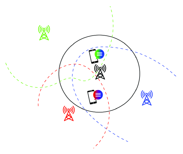
Although related to location discovery, the topic of this manuscript is the discovery of existing neighbours without targeting their actual geographical position. We focus on the process of NCLD via crowdsourcing, meaning that the task of detecting and reporting the existence of conflicting neighbours is delegated to users. In this framework, each user periodically reports to the serving node information about the set of neighbouring nodes observed, see e. g. Figure 1. Exploiting User Equipment (UE) measurements is appealing because such technique is easy to implement and virtually cost-free. Nevertheless, the information received from UE measurements is disregarded by the serving node in most implementations [2, §7.4.1].

Keeping the NCL updated is fundamental for a number of reasons:

• Neighbouring cells can be added, removed, or temporarily offline.

• The handover to a new cell might be problematic whenever it is not contained in the NCL of the serving cell.

• Some cells should not be added to the NCL list because they might reflect spurious measurements, yielding non-reliable handovers.

• Neighbours with same PCI should be handled with specific solutions.

With these reasons in mind, this manuscript studies the time $T$ necessary to achieve confident knowledge of the NCL through UE measurements. Estimating $T$ enables optimal tuning of neighbour cell list management schemes. $T$ is also important for the design and deployment of decentralised optimisation schemes. A key example is self-organisation, a problem where the network nodes need to optimise their configuration without a central controller, i. e. relying on local information only. There exist many fast and efficient decentralised algorithms to self-organise a WiFi/femtocell network; these algorithms are generally fed with a NCL, which needs to be constantly kept up-to-date. At implementation level, this means that each node needs to periodically estimate with a sufficient level of confidence which nodes of the network are potential conflicting neighbours. The majority of decentralised schemes require that each serving node needs local knowledge of the local neighbourhood [3, 4, 5, 6], and any attempt to relax this hypothesis comes at the expense of performance, as shown in Section II.

In the literature it is usually assumed that neighbourhood information may be instantaneously acquired [7, 8, 9, 10, 11, 12, 13], i. e. the time $T$ is considered negligible. In fact this assumption may often not be valid, either because it is necessary to listen to the channel long enough to get a high-confidence estimation or because hidden nodes/second-hop NCL need to be known as well, and thus it is necessary to use communication with users or other nodes to obtain such information. When the time needed by each serving node to update its NCL is larger than the time to execute the optimisation algorithm, a decentralised approach might not be the best solution.

In a framework where the NCL is built via crowdsourced user reports, our main goal is to rigorously characterise $T$ and study its properties and bounds. This is a problem that, to the best of our knowledge, has not yet been addressed in the literature. Our main contributions are the following: (i) the problem of user-reports-based NCLD is stated for the first time through a crisp mathematical formulation; (ii) we introduce a simple mobility model that is useful for gaining insight into those situations where crowdsourcing via user reports is likely to yield the greatest benefit to a decentralised approach; (iii) we show that this model can provide an upper bound on the time to topology discovery, thus it can be used as a design tool (see Section V-E).

Figure 1: Example of NCLD. Each user report to the serving node which neighbouring nodes they observe.

The rest of the paper is organised as follows: in Section II we present the related work, then, in Section III we show some practical use cases where our approach can be applied. In Section IV we provide a mathematical model for the discovery process and in Section V we define the problem in the context of such model and give some useful bounds. We present simulation results to validate the model and show how it can be used as a network design tool in Section VI. Finally, in Section VII we draw the conclusions.

II Related Work

In the field of decentralised algorithm design, it has been shown that local knowledge of network topology is enough to produce a distributed algorithm for resource allocation; such local knowledge also allows the minimisation of scrambling-code collision and confusion in small cell networks, see [14] and references therein. This knowledge is sufficient, and in a certain sense necessary to build efficient algorithms, as the attempts to relax the hypothesis that each serving node needs knowledge of the local neighbourhood will result in an extreme loss of performances [15, 16], that can be prevented only in specific scenarios where the interference model can be described with a simple graph [17].

Perhaps the main motivation of this manuscript is the work of [18], where the authors propose a neighbour cell list management scheme based on the long-term statistics of UE measurements. A key parameter of this scheme is the forgetting factor $\gamma$, that weigh the longitudinal UE measurements. Such parameter is clearly not trivial to tune, especially in settings, very common in wireless and cellular networking, where instantaneous cell list acquisition cannot be assumed. The optimal tuning $\gamma$ is only possible by studying the statistical properties of the time $T$ necessary to achieve confident knowledge of the NCL through UE measurements.

The user report function is already available in commercial femtocells [19] and small cells networks, and its implementation for code confusion and interference reduction is recommended in [14, 20].

Crowdsourcing approaches have been investigated for different applications, e. g. for estimating both density and number of attendees of large events [21]. Many works pertain the use of crowdsourcing for NCL discovery. In [22], the use of mobile measurement to update the NCL of macrocells after deployment has been studied: since the intra-frequency reporting function, known as Detected Set Reporting (DSR), is energetically costly for the mobile device, the use of it is suggested only in critical situations where a problem with the current NCL is known. A similar case, where the NCL needs to be updated when a new macrocell is deployed, is studied in [23]. Other ways to dynamically build the NCL via crowdsourcing are presented in [24, 18]. A similar work applied to WiMax is presented in [25], and a closely related approach for the femtocell case is presented in [26].

With this work, we address the problem of estimating the NCL construction time, which is necessary to assess whether crowdsourcing is effective in a particular network deployment. However, to the best of our knowledge, this problem has not been addressed in the literature yet.

III Use Cases

We show in this section some timely use cases where our proposed framework can be applied as a network design tool.

III-A 3G Network Optimisation

In order to provide seamless mobility and a satisfactory service, the optimisation of the handover function is fundamental in modern 3G cellular networks. To achieve that, the construction of a reliable NCL is one of the most critical tasks. While in the past this was achieved by drive and walk testing, the needs to adapt to changes in the network and to reduce the cost require different solutions [18, 12, 22].

The so-called DSR is an intra-frequency 3GPP functionality that allows users to report cells not defined in the NCL. In this way, whenever a macrocell detects a problem, or when a new cell is deployed [23], such a function can be activated. The only disadvantage is that such functionality is energetically costly for the mobile device, so its use is recommended for short periods of time and only in critical situations where a problem with the current NCL is known. Therefore, an estimation of the optimal time to keep the DSR active is required. Our work provides an effective framework to make such estimation possible.

III-B Small cells Self-configuration

An important problem that affects the small cells deployment for residential use is code selection. In 3G, basestations have only few scrambling codes available, making the task of selecting the optimal allocation challenging. Moreover, communication with a central controller is discouraged, to avoid signalling overhead. In 4G and 5G, Physical Cell Identity codes and 5G scrambling codes have similar problems.

A fully decentralised algorithm that can converge to the optimal confusion- and collision-free code allocation has been devised in [14]. However, it relies on the assumption that small cells are able to construct their NCL. Unfortunately, small cells are often not able to detect first- and second-hop neighbours reliably due to hidden-node effects and the absence of an efficient sniffing Common Pilot Channel (CPICH) mechanism. A technique to construct the NCL via crowdsourcing has been proposed by [26]. However, the implementation of such a technique would first require the evaluation of the time scale of the NCL construction and its comparison with the time scale of the convergence of the code allocation algorithm.

IV Neighbour Cell List Discovery Model

Given a set of wireless nodes ${\mathcal{A}}=\{a_{0},\dots,a_{N}\}$, let $A(a_{i})\subset\mathbb{R}^{2}$ denote the coverage area of access point $a_{i}$. Please note that $A(a_{i})$ generally depends on the transmission power of $a_{i}$ and on the radio propagation properties of the medium. We focus on serving access point $a_{0}$ and let ${\mathcal{B}}$ denote the neighbouring nodes that have non-void intersection with $A(a_{0})$, i. e.

$${\mathcal{B}}=\{a_{i}\in{\mathcal{A}},i>0\colon A(a_{0})\cap A(a_{i})\neq\emptyset\}.$$

We will hereafter use the symbol $N$ to denote the cardinality of ${\mathcal{B}}$, i. e. $N=|{\mathcal{B}}|$.

Let $\mathcal{P}({\mathcal{B}})$ denote the powerset of ${\mathcal{B}}$. A tessellation of the area $A(a_{0})$ is the collection of tiles $\{A_{\bm{i}}\}_{\bm{i}\in\mathcal{P}({\mathcal{B}})}$ such that

$$A(a_{0})=\bigcup_{\bm{i}\in\mathcal{P}({\mathcal{B}})}A_{\bm{i}}\,,$$ (1)

where

$$A_{\bm{i}}= \bigcap_{j\in\bm{i}}A(a_{j})\cap A(a_{0})\setminus\bigcup_{j\not\in\bm{i}}A(a_{j}),\quad\bm{i}\neq\emptyset,$$

$$A_{\emptyset}= A(a_{0})\setminus\bigcup_{\bm{i}\in\mathcal{P}({\mathcal{B}})\setminus\emptyset}A_{\bm{i}}.$$ (2)

In what follows each element $A_{{\bm{j}}}$ composing the tessellation is referred to as a tile, and we will use the vector notation ${\bm{j}}$ to represent a set of neighbouring nodes. Let us consider for example $\bm{i}=\{a_{1},a_{2}\}$; then, the tile $A_{\bm{j}}$ is the portion of $A(a_{0})$ that is covered by $a_{1}$ and $a_{2}$ only, see Figure 2.

Figure 2: Example of tesselation corresponding to scenario of Figure 1. The scenario is modelled with a serving node, $a_{0}$, with three interfering neighbours, $a_{1},a_{2},$ and $a_{3}$; the coverage area of the serving node, $A(a_{0})$, can be tessellated with the sets $A_{0},A_{1},A_{2},A_{3},A_{12},A_{13},A_{23},A_{123}$. For simplicity of notation, we will write $A_{0}\coloneqq A_{\emptyset}$.

Figure 3: Hypercube representation of the tessellation for $N=4$. There is one zeroth order tile, namely $A^{C}$, four first order tiles, $A_{1},A_{2},A_{3}$ and $A_{4}$, six second order tiles, $A_{12},A_{13},A_{14},A_{23},A_{24},A_{34}$, four third order tiles, $A_{123},A_{124},A_{134},A_{234}$ and a fourth order tile, i. e. $A_{1234}$.

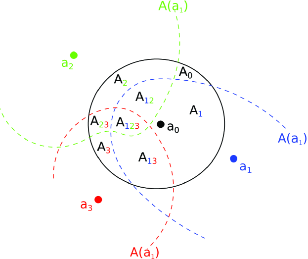
Whenever a user is in $A_{\bm{j}}$, it will report $\bm{j}$ to access point $a_{0}$. In other words, $a_{0}$ will be aware of the existence of those neighbouring nodes $a_{i}\in\bm{j}$. The rate of these reports depends on the mobility model assumed (see Section V).

To keep the model as conservative as possible, and to encompass the frequent case of half-duplex nodes, we assume $a_{0}$ cannot detect the existence of any neighbour even though $a_{0}$ lies in one of the neighbours coverage area.

Let $\mathcal{K}_{t}$ denote the knowledge set of access point $a_{0}$, i. e. the set of neighbours that $a_{0}$ is aware of, at time $t$. Given a sequence of reports $\{\bm{j}^{1},\dots,\bm{j}^{t}\}$, we have that $\mathcal{K}_{t}=\bigcup_{i=1}^{t}\bm{j}^{i}$. $\mathcal{K}_{t}$ is a sequence of sets that satisfies

$$\mathcal{K}_{t}=\bigcup_{s=0}^{t}\mathcal{K}_{s};$$ (3)

in particular, $\mathopen{}\mathclose{{}\left\lvert\mathcal{K}_{t}}\right\rvert$ is non-decreasing in $t$. Clearly, the knowledge state at time $t$, $\mathcal{K}_{t}$, take values in $\mathcal{P}({\mathcal{B}})$.

Definition 1 (Full Knowledge).

Given an integer $T$ and a finite sequence of reports $\{\bm{j}^{1},\dots,\bm{j}^{T}\}$, the node $a_{0}$ is said to have Full Knowledge (FK) of its neighbours at time $T$ if

$$\mathcal{K}_{T}=\bigcup_{s=1}^{T}\bm{j}^{s}={\mathcal{B}}.$$

Remark 1.

If $a_{0}$ has Full Knowledge (FK) of its neighbours at time $T$, so it has at all times $T+t$ for $t\geq 0$. In other words, once $a_{0}$ has reached FK, it cannot lose it.

Definition 2 (First time to FK).

Given a sequence of reports $\{\bm{j}^{1},\bm{j}^{2},\dots\}$, the first time to FK $\tau$ for the node $a_{0}$ is the first time the latter reaches FK of its neighbours, i. e.

$$\tau\coloneqq\min\{T\geq 0\text{ such that }\mathcal{K}_{T}={\mathcal{B}}\}\,.$$ (4)

Remark 2.

The characterisation of the first time to FK generally depends on the realisation of a sequence of user reports; this means that $\tau$ is a random variable. More precisely, by (4), $\tau$ is a stopping time, see e. g. [27].

We end the section with a note on the tessellation:

Remark 3.

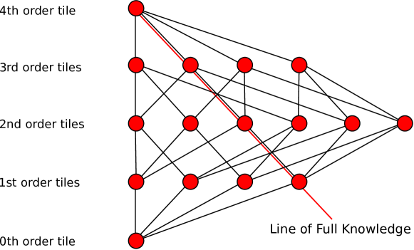
A generic tessellation of ${\mathcal{B}}$ can be represented as a hypercube $H=\{0,1\}^{N}$ by identifying the vertices of $H$ with the tiles $A_{\bm{j}}$ that the tessellation is composed of. The number of tiles of a generic tessellation of ${\mathcal{B}}$ is $2^{N}$ as well as the vertices of a hypercube, represented as vectors of size $N$. The tiles of the tessellation can be mapped onto the vertices of the hypercube by identifying the $i$-th component of the vertices $x\in H$ with $a_{i}\in{\mathcal{B}}$. In other words,

$$A_{\bm{j}}\leftrightarrow x\quad\Leftrightarrow\quad x_{i}=\mathds{1}_{\{a_{i}\in{\bm{j}}\}}\,,\;i=1,\ldots,N,$$

where $\mathds{1}$ is the indicator function. We define the order of a tile as the number of neighbours a report from that tile would give knowledge of; the number of $k$-th order tiles is ${N\choose k}$. A report from a $k$-th order tile is equivalent to $k$ first-order reports. In particular, FK is attained with a report from the $N$-th order tile, or at least two reports from two distinct $(N-1)$-th tiles, etc. This property can be graphically represented by what we call the Line of Full Knowledge, see Figure 3. The line of FK is clearly not unique; the aim of Figure 3 is only to illustrate that a sequence of $T$ reports $\{\bm{j}^{1},\dots,\bm{j}^{T}\}$ is a path on the hypercube $H$, and that FK is attained whenever a line of FK is reached at a time smaller than $T$.

Since $\mathcal{K}_{t}$, the knowledge state at time $t$, takes on values in the same set $\mathcal{P}({\mathcal{B}})$, we can also map the knowledge states on the hypercube $H$. That is, a sequence of reports $\{\bm{j}^{1},\bm{j}^{2},\dots,\bm{j}^{t}\}$ is equivalent to a single report from tile $\bigcup_{s=1}^{t}\bm{j}^{s}=\mathcal{K}_{t}$.

We can now define the main problems of this work.

Problem 1 (Expected first time to Full Knowledge).

Given an access point $a_{0}$, a set ${\mathcal{B}}$ of neighbours with given position and coverage area, and a sequence of user reports, we want to characterise the expectation of the first time to FK, i. e.

$$\mathbb{E}(\tau)=\sum_{t\geq 1}t\,\mathbb{P}(\tau=t)\,.$$

Obviously, the way the user(s) moves inside the coverage area $A(a_{0})$ heavily affects the difficulty of the problem and its answer. However, the formulation of Problem 1 has the great advantage of decoupling the notion of FK from the user mobility model; addressing the mean value of the first time to FK is also an enabler to the estimate of the tail of the distribution of $\tau$ – through Markov’s inequality, for example. Further, from a numerical point of view, the expected time to FK may be achieved via a Monte Carlo simulation once the set ${\mathcal{B}}$ and the mobility model in use are fixed.

There may exist cases where it is only necessary to characterise the first time to attain partial knowledge of the local topology. For example, we may be interested in the first moment when the neighbouring nodes that have been already discovered, i. e.  the elements of the knowledge set $\mathcal{K}_{t}$, are enough to describe a given fraction of the local topology. This idea motivates the following

Problem 2 (Expected first time to $\delta$-knowledge).

Let $\varrho$ be a measure over $\mathcal{P}({\mathcal{B}})$ and fixed $\delta\in(0,1]$. Given an access point $a_{0}$, a set ${\mathcal{B}}$ of neighbours with given position and coverage area, and a sequence of user reports, we want to characterise the expectation of the first time to $\delta$-knowledge $\mathbb{E}(\tau_{\delta})$, where

$$\tau_{\delta}=\min\mathopen{}\mathclose{{}\left\{T\geq 0\text{\emph{ such that }}\frac{\sum\limits_{\bm{k}\in\operatorname{\mathcal{P}}(\mathcal{K}_{T})}\varrho\mathopen{}\mathclose{{}\left(A_{\bm{k}}}\right)}{\sum\limits_{\bm{j}\in\operatorname{\mathcal{P}}({\mathcal{B}})}\varrho\mathopen{}\mathclose{{}\left(A_{\bm{j}}}\right)}\geq\delta}\right\}\,.$$

When $\delta=1$ and $\varrho(A_{\bm{j}})>0$ for each $\bm{j}\in\operatorname{\mathcal{P}}({\mathcal{B}})$, Problem 2 is equivalent to Problem 1. Indeed, $\nicefrac{{\sum\limits_{\bm{k}\in\operatorname{\mathcal{P}}(\mathcal{K}_{T})}\varrho\mathopen{}\mathclose{{}\left(A_{\bm{k}}}\right)}}{{\sum\limits_{\bm{j}\in\operatorname{\mathcal{P}}({\mathcal{B}})}\varrho\mathopen{}\mathclose{{}\left(A_{\bm{j}}}\right)}}\geq 1$ if and only if $\mathcal{K}_{T}\equiv{\mathcal{B}}$.

We will hereafter consider the Lebesgue measure $\varrho(A_{\bm{k}})=\mathopen{}\mathclose{{}\left\lVert A_{\bm{k}}}\right\rVert$. This leads to the following interpretation: $\delta$-knowledge is attained when the knowledge set $\mathcal{K}_{t}$ defines for the first time a tessellation that covers a fraction of $A(a_{0})$ larger or equal than $\delta$. Equivalently, $\tau_{\delta}$ is the first time when the tiles that would give new information cover a fraction of $A(a_{0})$ that is smaller than $1-\delta$.

Remark 4.

The concept of $\delta$-knowledge is fundamental in the simulation phase, when we want to know whether user reports can effectively be used to give knowledge of the local topology. Indeed, it is likely that the neighbours $a_{i}$ whose coverage area do not overlap with $A(a_{0})$ save for a nearly negligible portion, will be discovered after a very long time; in other words, the leading contribution to $\mathbb{E}(\tau)$ will be represented by the mean first visit time of the user(s) to $A(a_{i})$. Discarding $a_{i}$ from the picture, the concept of $\delta$-knowledge let us focus on the quantitative analysis of NCLD, see Section VI.

V Teleport Mobility

The characterisation of $\tau$, the first time to FK, depends on the assumed user’s mobility model: it describes how users enter, exit, and move within $A(a_{0})$. The users evolution can then be represented as a pair $U_{t}=(n_{t},X_{t})$, where $n_{t}$ is the number of users that lie in $A(a_{0})$ at time $t$, and $X_{t}=(x_{t}^{1},x_{t}^{2},\ldots,x_{t}^{n_{t}})$ is a vector with the position of the $n_{t}$ users. We assume the evolution of $U_{t}$ to be driven by a discrete-time Markov chain (MC) throughout the paper.

The realisation of $\{U_{t}\}_{0\leq t\leq T}$ completely determines the sequence of user reports $\{\bm{j}^{1},\dots,\bm{j}^{T}\}$ to the access point $a_{0}$, cf. Remark 2. Since $\mathcal{K}_{t}$ only depends on $\mathcal{K}_{t-1}$ and $U_{t}$, then the bivariate process $(U_{t},\mathcal{K}_{t})$ is a MC.

It will prove useful to consider a simplified mobility model in which a single user continuously teleport between tiles, without leaving $A(a_{0})$:

Model 1.

(Teleport Mobility) A single user moves within $A(a_{0})$ according to a discrete-time MC taking on values in $\mathcal{P}({\mathcal{B}})$. At any time the user cannot abandon the whole region, i. e. it is constrained within $A(a_{0})$. At each step, the user instantaneously teleports with a probability that is proportional to the measure of the destination tile. The destination tile can also be the same tile of previous step, meaning that the user would remain on the same tile during that discrete time step. Assuming that all tiles are Lebesgue-measurable plane sets, the transition probabilities are

$$\operatorname{\mathbb{P}}\mathopen{}\mathclose{{}\left(\bm{i}\rightarrow\bm{j}}\right)=\frac{\lVert A_{\bm{j}}\rVert}{\lVert A(a_{0})\rVert},$$ (5)

where $\lVert\cdot\rVert$ denotes the Lebesgue measure.

Remark 5.

Model 1 greatly simplifies the characterisation of $\tau$, the first time to FK. Indeed, in this mobility model, $\mathcal{K}_{t}$ is independent of $U_{t}$, and the sole process $\mathcal{K}_{t}$ is hence sufficient to describe the process of gathering knowledge from the user reports. We will hereafter refer to $\mathcal{K}_{t}$ as the knowledge chain.

Assuming Model 1, we can easily describe the process of gathering knowledge from user reports as a discrete-time random walk on the hypercube $H=\{0,1\}^{N}$ (which we have introduced in Remark 3); having knowledge of $n$ neighbouring nodes is in fact equivalent to receiving a report from the $n$-th order tile that give information about all of them.

Let $P(\cdot,\cdot)$ be the transition kernel of the knowledge chain. If $\bm{k}\not\subseteq\bm{l}$, then (3) guarantees that $P(\bm{k},\bm{l})=0$ because such transition would mean a loss of knowledge. Conversely, when $\bm{k}\subseteq\bm{l}$, a transition from $\bm{k}$ to $\bm{l}$ happens if the user moves to a tile that contains the missing information $(\bm{l}\setminus\bm{k})$ and does not add more information than that. Therefore,

$$P(\bm{k},\bm{l})=\begin{cases}\sum\limits_{\bm{m}\in\mathcal{P}(\bm{k})}\frac{\mathopen{}\mathclose{{}\left\lVert A_{\{\bm{m}\cup(\bm{l}\setminus\bm{k})\}}}\right\rVert}{\lVert A(a_{0})\rVert}&\text{if $\bm{k}\subseteq\bm{l}$},\\ \qquad 0&\text{otherwise}.\end{cases}$$ (6)

The following result holds:

Lemma 1.

The matrix $P$ is upper triangular.

Proof:

Let us consider the following partial ordering relation among the states:

$$\bm{k}\preceq\bm{l}\quad\Leftrightarrow\quad\bm{k}\subseteq\bm{l}\,.$$

By (6), $P(\bm{k},\bm{l})\neq 0$ only if $\bm{k}\preceq\bm{l}$. Therefore, any mapping

$$\mathcal{P}({\mathcal{B}})\ni\bm{l}\quad\leftrightarrow\quad l\in\{1,2,\ldots,2^{N}\}$$

such that

$$\bm{k}\preceq\bm{l}\quad\Leftrightarrow\quad k\leq l$$

will put the matrix $P$ into an upper triangular form. In particular, we can order the states by increasing cardinality and in lexicographic order. ∎

The explicit computation of the whole matrix $P$ using (6) is expensive in general since $P$ is a $2^{N}\times 2^{N}$ matrix. However, as stated above, $P$ is upper triangular. In Section V-C we show that it is possible to explicitly characterise its spectrum. For the reader’s reference, Table I shows the matrix $P$ for $N=3$.

$P=\frac{1}{\lVert A(a_{0})\rVert}\begin{pmatrix}\lVert A_{0}\rVert&\lVert A_{1}\rVert&\lVert A_{2}\rVert&\lVert A_{3}\rVert&\lVert A_{12}\rVert&\lVert A_{13}\rVert&\lVert A_{23}\rVert&\lVert A_{123}\rVert\\ 0&\lVert A_{0}\rVert+\lVert A_{1}\rVert&0&0&\lVert A_{2}\rVert+\lVert A_{12}\rVert&\lVert A_{3}\rVert+\lVert A_{13}\rVert&0&\lVert A_{23}\rVert+\lVert A_{123}\rVert\\ 0&0&\lVert A_{0}\rVert+\lVert A_{2}\rVert&0&\lVert A_{1}\rVert+\lVert A_{12}\rVert&0&\lVert A_{3}\rVert+\lVert A_{23}\rVert&\lVert A_{13}\rVert+\lVert A_{123}\rVert\\ 0&0&0&\lVert A_{0}\rVert+\lVert A_{3}\rVert&0&\lVert A_{13}\rVert+\lVert A_{1}\rVert&\lVert A_{2}\rVert+\lVert A_{23}\rVert&\lVert A_{12}\rVert+\lVert A_{123}\rVert\\ 0&0&0&0&\lVert A_{0}\rVert+\lVert A_{1}\rVert+\lVert A_{2}\rVert+\lVert A_{12}\rVert&0&0&\lVert A_{3}\rVert+\lVert A_{13}\rVert+\lVert A_{23}\rVert+\lVert A_{123}\rVert\\ 0&0&0&0&0&\lVert A_{0}\rVert+\lVert A_{1}\rVert+\lVert A_{3}\rVert+\lVert A_{13}\rVert&0&\lVert A_{2}\rVert+\lVert A_{12}\rVert+\lVert A_{23}\rVert+\lVert A_{123}\rVert\\ 0&0&0&0&0&0&\lVert A_{0}\rVert+\lVert A_{2}\rVert+\lVert A_{3}\rVert+\lVert A_{23}\rVert&\lVert A_{1}\rVert+\lVert A_{12}\rVert+\lVert A_{13}\rVert+\lVert A_{123}\rVert\\ 0&0&0&0&0&0&0&1\end{pmatrix}.$

Table I: Example of transition matrix $P$ for $N=3$.

V-A Expected Time to Full Knowledge

Let $\bm{k}^{\ast}=\{1,2,\ldots,N\}$ be the state of FK. By formula (6), $P(\bm{k}^{\ast},\bm{k}^{\ast})=1$. This means that the chain has an absorbing state, and the hitting time of this state is just $\tau$, the first time to FK. Hence, we can compute the expected time to FK simply by

$${\operatorname{\mathbb{E}}\mathopen{}\mathclose{{}\left[\tau}\right]}=(I-Q)^{-1}\mathbf{1},$$ (7)

where $Q$ is obtained from $P$ by removing the row and the column relative to state $\bm{k}^{\ast}$ and $\mathbf{1}$ is the column vector of ones [28]. In a similar way, it is possible to compute the other moments of $\tau$.

Even if $I-Q$ is upper triangular and can be block decomposed, the computation of its inverse may not be affordable when the cardinality of ${\mathcal{B}}$ grows. In Section V-D we will bound the probability of the event $\{\tau>t\}$.

V-B Expected Time to $\delta$-knowledge

Regarding Problem 2, we can easily modify matrix $P$ to obtain the expected time to $\delta$-knowledge. Every state $\bm{k}\in\operatorname{\mathcal{P}}({\mathcal{B}})$ such that

$$\sum\limits_{\bm{l}\in\operatorname{\mathcal{P}}(\bm{k})}\frac{\mathopen{}\mathclose{{}\left\lVert A_{\bm{l}}}\right\rVert}{\lVert A(a_{0})\rVert}\geq\delta$$

can be aggregated in the absorbing state, summing the corresponding column of $P$ in the last column, and then eliminating the column and row corresponding to state $\bm{k}$. In this way it is possible to compute ${\operatorname{\mathbb{E}}\mathopen{}\mathclose{{}\left[\tau_{\delta}}\right]}$ using (7).

V-C Eigenvalues

The following result fully characterises the spectrum of the matrix $P$:

Theorem 2.

For $\bm{k}\in\mathcal{P}({\mathcal{B}})$, the eingenvalues of $P$ have the form

Proof:

The matrix $P$ being upper triangular by Lemma 1, the entries $P(\bm{k},\bm{k})$ are the eigenvalues of the matrix. Let us then imagine to have the knowledge chain in state $\bm{k}$. The only way for the chain to undergo a self-transition ($\bm{k}\to\bm{k}$) is that the user reports any combination of neighbouring nodes that have already been discovered. In other words, the knowledge chain undergoes a self-transition if and only if the user reports an element of $\mathcal{P}(\bm{k})$. Therefore,

$$\lambda_{\bm{k}}=\frac{1}{\lVert A(a_{0})\rVert}\sum_{\bm{l}\in\mathcal{P}(\bm{k})}|A_{\bm{l}}|\,.$$

Last formula is equivalent to the thesis. ∎

Since each eigenvalue is a sum of positive elements, the second-largest eigenvalue $\tilde{\lambda}$ can be obtained by maximising over the tiles of order $N-1$:

$$\tilde{\lambda}=\max_{\bm{k}\colon\lvert\bm{k}\rvert=N-1}\lambda_{\bm{k}}.$$ (8)

V-D Convergence Properties, Bounds

Using (8), it is possible to obtain the following result:

Lemma 3.

Given $\varepsilon>0$, let

$$S(1-\varepsilon)=\frac{\log{\varepsilon}}{\log{\tilde{\lambda}}}.$$ (9)

Then, $S(1-\varepsilon)$ reports are sufficient to achieve FK with probability greater or equal than $(1-\varepsilon)$.

Proof.

Using Lemma 1 and Equation (8) on $P$,

$$\operatorname{\mathbb{P}}\mathopen{}\mathclose{{}\left(\tau>t}\right)\leq\tilde{\lambda}^{t}.$$ (10)

For a small target tolerance $\varepsilon$ of not achieving FK,

$$\text{if }t\geq\frac{\log{\varepsilon}}{\log{\tilde{\lambda}}}\quad\Rightarrow\quad\operatorname{\mathbb{P}}\mathopen{}\mathclose{{}\left(\tau>t}\right)\leq\varepsilon.$$ (11)

∎

$\delta$-knowledge Convergence Bounds

Using the same manipulation of the matrix $P$ described in Section V-B, Corollary 3 can be applied to the modified matrix to obtain a bound for the number of steps to have $\delta$-knowledge with high probability.

V-E $\delta$-knowledge and other-than-teleport mobility

Model 1 is equivalent to a single user teleporting instantaneously to a random point within the coverage area of the node; time is discrete. Thus, at each time the node $a_{0}$ receives a user report from a point drawn according to the uniform probability distribution over the coverage area $A(a_{0})$. Having in mind the numerical characterisation of the first time to $\delta$-knowledge, the teleport model is particularly convenient. This task could be in fact carried out within the Monte Carlo paradigm by simply throwing sufficiently many points at random inside the coverage area $A(a_{0})$. In other words, it is possible to numerically study the process through which $\delta$-knowledge is achieved by sampling sufficiently many times a probability density function that is uniform over the coverage area $A(a_{0})$.

Model 1 may prove itself unsatisfactory in a real life scenario. The main problem is that if we generate a sequence of user reports according to it, any two elements of the sequence are independent, whereas in general they are not. In each mobility model where the trajectory taken by the user is physically feasible, the user positions communicated by two successive reports are in fact correlated due to the motion constraints.

Let us imagine that a single user travels inside the coverage area $A(a_{0})$ according to an unknown mobility model, and let $T(t)$ be the trajectory taken by the user. Sampling the trajectory at equally-spaced discrete times, we obtain an embedded sequence of user locations, which correspond to an embedded sequence of user reports. Next, we can analyse the sequence and understand after how many steps $\delta$-knowledge has been reached. By multiplying this number of steps by the time lapse between two consecutive reports (inter-report time), the time to $\delta$-knowledge can be obtained for that particular realisation of the user-reports sequence. Finally, the procedure above can be repeated sufficiently many times to estimate with a Monte Carlo method the expected time necessary for $a_{0}$ to reach $\delta$-knowledge.

As mentioned above, in a general mobility model it is likely that two successive user reports are correlated. These correlations may decay as the inter-report time grows larger and larger. As an example, let us imagine that a single user travels inside the coverage area $A(a_{0})$ according to a MC. Let $\pi$ be the equilibrium probability measure of the chain and let $t_{\text{mix}}$ be the mixing time of the chain, i. e. the time needed for the chain to reach equilibrium. If the inter-report time is chosen comparable to $t_{\text{mix}}$ then the time lapse between two successive reports will be sufficient for the MC to forget the past trajectory; in other words, the correlations between consecutive reports will be negligible. As a consequence, the user locations will be independently drawn from the probability measure $\pi$, and the matrix $P$ describing the knowledge evolution will become

$$P(\bm{k},\bm{l})=\begin{cases}\sum_{\bm{m}\in\mathcal{P}(\bm{k})}\pi\mathopen{}\mathclose{{}\left(A_{\{\bm{m}\cup(\bm{l}\setminus\bm{k})\}}}\right)\quad&\text{if }\bm{k}\subseteq\bm{l},\\ 0&\text{otherwise.}\end{cases}$$ (6’)

Therefore, the formulation and the results developed in Sections V-A–V-D are still valid if we consider a single-user mobility model based on a MC, provided that the time lapse between two consecutive reports is of the order of the mixing time of the chain. Under the assumption that user reports are sent at a frequency comparable with the inverse mixing time of the mobility MC, we can compute an upper bound on the time to $\delta$-knowledge. Any reporting rate higher than $\tfrac{1}{t_{\text{mix}}}$ will in fact still guarantee that $a_{0}$ achieves $\delta$-knowledge of its neighbourhood in at most ${\operatorname{\mathbb{E}}\mathopen{}\mathclose{{}\left[\tau_{\delta}}\right]}\cdot t_{\text{mix}}$ seconds on average.

V-E1 Multi-user Scenario

We end this section by briefly mentioning a straightforward application of Model 1 in a multi-user scenario. Let us imagine that $n$ users may enter, move within, and exit $A(a_{0})$ according to a hidden mobility model. We assume that $n$ is a very large number and that it is possible to statistically characterise the stationary user-density by means of a probability measure $\pi$ over $A(a_{0})$. At each time every user may independently send a report with a very small probability $p$. Then, the number of reports received by $a_{0}$ in a given time interval is approximately Poissonian and the time lapse between two successive reports is exponential with parameter $\lambda=np$. Next, let $m={\operatorname{\mathbb{E}}\mathopen{}\mathclose{{}\left[\tau}\right]}$ be the expected time to FK, expressed in number of reports, returned by (6’) and (7); the expected time to achieve FK is the expectation of the first time for a Poisson process of parameter $\lambda$ to hit the state $m$. A practical example for this kind of scenario in presented in Section V-F2.

V-F Examples

V-F1 Femtocells Deployment for Residential Use

Regarding the use case of femtocell self-organisation presented in Section III-B, each basestation serves a very small number of devices. Using data of typical residential densities and coverage areas, a statistic of the tessellation can be devised. If it is possible to establish a time $\tilde{T}$ after which the user position can be considered as drawn from a uniform distribution, then $S(\delta)$ is an upper bound of the time to $\delta$-knowledge for all the inter-report times smaller than or equal to $\tilde{T}$.

V-F2 Cells Deployed in Congested Areas

Opposite to the previous example, cells deployed in congested places like a mall have an extremely large basin of potential users. However, in situations where users main interest is other than connecting to the internet, it is reasonable to expect the single-user reporting-activity to be rather sporadic. Therefore, the Poissonian approximation that we have mentioned at the end of Section V-E may be applicable. In this case, characterising the time to achieve $\delta$-knowledge is possible through a statistic of the typical (or worst case) tessellations.

VI Simulations

VI-A Teleport Model on Random Positioned Nodes

In this section we offer a preliminary assessment of the possibility to use the machinery developed so far in real applications. To this purpose, we developed a simulation framework in MATLAB and studied a scenario where $8$ nodes are positioned on a plane at random according to a uniform (bivariate) probability distribution, i.e. uniformly at random. Each node has a circular coverage area of the same size. We considered $350$ different configurations, with the constraint that the coverage area of $a_{0}$ has non-void intersection with the coverage area of the remaining nodes, meaning that FK is achieved as soon as all $7$ neighbours are reported to $a_{0}$. We compute the tessellation of each configuration using a classical Monte Carlo sampler. For each of these $350$ configurations, we computed the expected time to $0.9$-knowledge ${\operatorname{\mathbb{E}}\mathopen{}\mathclose{{}\left[\tau}\right]}$ together with the number of steps sufficient to guarantee $0.9$-knowledge with $90\text{\,}\mathrm{\char 37\relax}$ confidence, i. e. $S(0.9)$. The inter-report time being fixed during this first experiment, the amount of time in seconds to achieve $0.9$-knowledge is directly proportional to the number of steps just evaluated.

Figure 4 displays the empirical probability mass function of these two quantities. ${\operatorname{\mathbb{E}}\mathopen{}\mathclose{{}\left[\tau}\right]}$ is centered around $10$ steps, while $S(0.9)$ is shifted on higher values, as expected being an upper bound.

Figure 4: Empirical probability mass function of the expected time to $0.9$-knowledge, and the number of steps to have $0.9$-knowledge with $90\text{\,}\mathrm{\char 37\relax}$ confidence, for the teleport model on random positioned nodes. Since the inter-report time is fixed, the simulation time is directly proportional to the number of reports.

Figure 5: Empirical cumulative distribution function of the expected time to $0.9$-knowledge, and the number of steps to have $0.9$-knowledge with $90\text{\,}\mathrm{\char 37\relax}$ confidence, for the teleport model on random positioned nodes. Since the inter-report time is fixed, the simulation time is directly proportional to the number of reports.

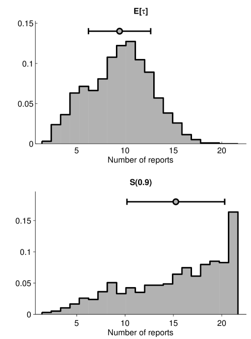
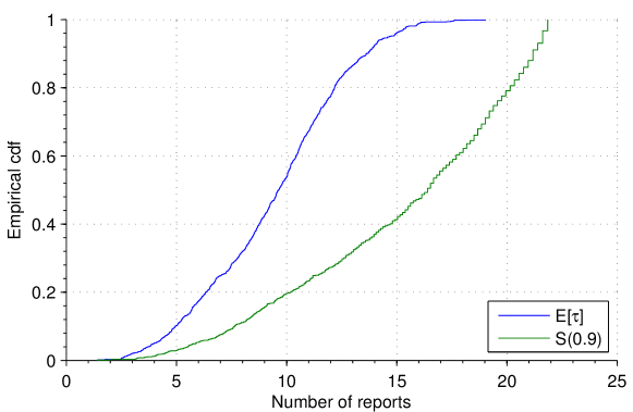
Figure 5 shows the empirical cumulative distribution function of ${\operatorname{\mathbb{E}}\mathopen{}\mathclose{{}\left[\tau}\right]}$ and $S(0.9)$. We see that $16$ steps are sufficient to achieve $0.9$-knowledge for nearly all scenarios ($95\text{\,}\mathrm{\char 37\relax}$), while we need $22$ steps using $S(0.9)$. We also notice that the bound obtained from (9) is a conservative estimation, because it uses only the second-largest eigenvalue $\tilde{\lambda}$. Indeed, it takes into account only the slowest way to reach the desired knowledge, while the problem has a rich combinatorial structure that cannot be completely captured by (10).

Roughly speaking, a user moving at $0.5\text{\,}\mathrm{m}\mathrm{/}\mathrm{s}$ according to a random walk model, and providing at least one report every hour, can guarantee the node will have $0.9$-knowledge with high probability in less than $5\text{\,}\mathrm{h}$, and in less than two hours if reports are sent at least every 15 minutes (see next section for a more detailed analysis on the interaction between report frequency and our bound). If the local topology is not typically expected to change often, these are acceptable times.

To summarise, simulation on random scenarios show that our proposed bound can be used to estimate the time to $\delta$-knowledge. Using realistic values, the expected time to $\delta$-knowledge is reasonably small.

VI-B Random Walk on a Grid

In order to investigate and confirm the ideas of Section V-E, we simulated the reports sent with different inter-report times by a random walker that moves within $A(a_{0})$ under the condition of reflective boundary, and compared this mobility model with Model 1 (see Section V) for a set of 8 nodes positioned as described at the beginning of this section.

Figure 6: Empirical mean $0.9$-knowledge time (in hours) of a random walk vs. inter-report period, compared with Model 1 and its bound $S(0.9)$ in a femtocell grid of 8 nodes.

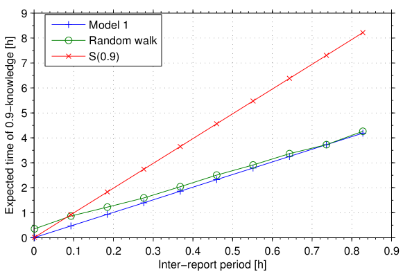
In Figure 6 we let the inter-report time increase and compare the average time to achieve $0.9$-knowledge according to both the random walk (green line) and the teleport model (blue). We see that that, if the inter-report time is sufficiently large, the empirical mean time to achieve $0.9$-knowledge for the random walk model is well approximated by that of Model 1.

We assume typical femtocell parameters, i. e. that coverage radius is $50\text{\,}\mathrm{m}$ and that the user do a step in a grid of $2.5\text{\,}\mathrm{m}$ every $5\text{\,}\mathrm{s}$. Figure 6 also shows that when reports are sent each $6\text{\,}\mathrm{m}\mathrm{i}\mathrm{n}$ or less, the time to 0.9-knowledge is smaller than $1\text{\,}\mathrm{h}$, but at such high frequency the bound $S(0.9)$ (red line) is not valid anymore. The reason why more reports than Model 1 are needed in the case of high-frequency reports is the following: since the inter-report time is short, it is likely that many reports will be sent from the same tile, i. e. the knowledge chain will undergo many self-transitions.

It is important to notice that the inter-report time used in Figure 6 are far from the theoretical order of magnitude of the random walk mixing time. Yet Figure 6 suggests that, for a family of scenarios, it should be possible to determine the value of the inter-report time such that the average time to achieve $0.9$-knowledge may be well predicted by Model 1. Once that value of the inter-report time is found, the value of $\mathbb{E}[\tau_{0.9}]$ returned by Model 1 may serve as an upper bound to the actual time to achieve $0.9$-knowledge when smaller inter-report times are implemented.

To summarise, simulation on random walks corroborate the analysis of Section V-E

VI-C A Realistic Scenario

A received power map for 4 basestations in the Hynes convention centre have been generated using the Wireless System Engineering (WiSE) [29] software, a comprehensive 3D ray tracing based simulation package developed by Bell Laboratories.

Figure 7: Coverage areas at Hynes convention centre. The coloured lines delimit the extension of the coverage areas. Basestations are transmitting at $2.1\text{\,}\mathrm{GHz}$ with a power of $34\text{\,}\mathrm{mW}$. Point $a$ lies in the tile $A_{123}$.

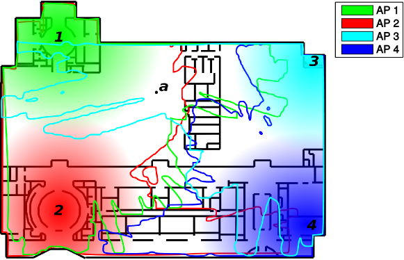
Basestations are assumed transmitting at a frequency of $2.1\text{\,}\mathrm{GHz}$ with a power of $34\text{\,}\mathrm{mW}$. We assume there is a macrocell that covers the whole building, and we estimate its time to full knowledge. As before, a Monte Carlo simulation has been made to estimate the tessellation, and then the expected time to $\delta$-knowledge has been computed using a teleport mobility model (Model 1), as explained in Section V-B.

Figure 7 shows the corresponding coverage areas when the power detection threshold is $-70\text{\,}\mathrm{dBm}$. Although the shape of the coverage areas and their intersection is much more complex than the simple scenario depicted in Section VI-A, it is still possible to construct the tessellation by considering which coverage areas each spatial point lies in. For example, point $a$ lies in the coverage area of nodes $1$, $2$, and $3$, so it belongs to the tile $A_{123}$.

Figure 8 displays the expected time to $\delta$-knowledge, ${\operatorname{\mathbb{E}}\mathopen{}\mathclose{{}\left[\tau_{\delta}}\right]}$ when $\delta$ is varied. We notice a step-function-like behaviour, with a new step that is added every time a new state become absorbing, as explained in Section V-B.

Figure 8: Expected time to $\delta$-knowledge, ${\operatorname{\mathbb{E}}\mathopen{}\mathclose{{}\left[\tau_{\delta}}\right]}$ using Model 1 in Hynes convention centre for different values of the parameter $\delta$. The inter-report time is set to the very same value used for Figures 4 and 5.

Figure 9: Expected time to FK, ${\operatorname{\mathbb{E}}\mathopen{}\mathclose{{}\left[\tau}\right]}$, using Model 1 in Hynes convention centre, for different values of the user-detection threshold. The inter-report time is set to the very same value used for Figures 4 and 5.

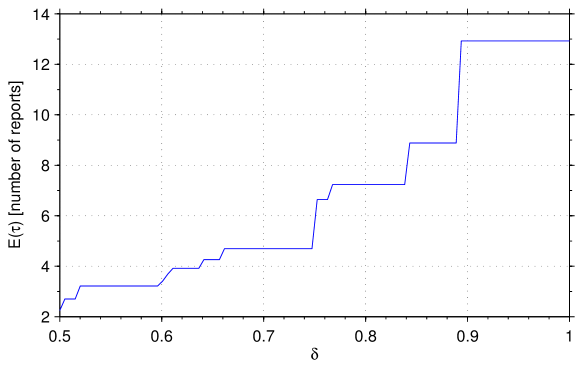
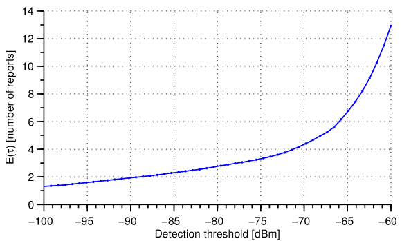
Figure 9 shows the behaviour of ${\operatorname{\mathbb{E}}\mathopen{}\mathclose{{}\left[\tau}\right]}$, the expected time to FK, when the user detection threshold varies from a very conservative value of $-60\text{\,}\mathrm{dBm}$ to a more realistic one of $-100\text{\,}\mathrm{dBm}$. When the users are more sensitive, the coverage areas, and specifically the higher order tiles, are bigger, leading to better performance. In particular, we see that an average of 14 steps are enough to achieve FK.

To summarise, these results seem to confirm that the values obtained placing random nodes with circular coverage areas in Section VI-A are compatible with real world scenarios, so the use of statistics obtained from macroscopic parameters as densities of deployment and distribution of coverage radii can be used as a tool to bound the time to $\delta$-knowledge.

VII Conclusions

In this paper, we have introduced the problem of user-reports-based Neighbour Cell List Discovery and provided a crisp mathematical formulation of it for a simple mobility model. We have also shown that such mobility model can be effectively used as an upper bound for a wide range of mobility models when the user reports frequency is lower than the inverse mixing time of the Markov chain of the actual mobility model. Additionally, we have provided a useful method to estimate the time to $\delta$-knowledge when the problem is too complex to be solved exactly.

Simulations on random scenarios with typical small cells parameters show that the expected number of reports in order to have a high degree of knowledge of the local topology is very small. Roughly speaking, a user moving at $0.5\text{\,}\mathrm{m}\mathrm{/}\mathrm{s}$ according to a random walk model, and providing at least one report every hour, can guarantee the serving node will have $0.9$-knowledge with high probability in less than $5\text{\,}\mathrm{h}$, and in less than two hours if reports are sent at least every 15 minutes. Since we do not expect the network topology to be affected by high network dynamics, these are acceptable times for the problems of interest. We encourage the adoption of the presented framework to assess the possibility of employing crowdsourced user reports in other self-configuration problems, comparing the time to $\delta$-knowledge with the expected time to convergence of a given decentralised algorithm.

Simulations in more realistic scenarios show that the bounds obtained are compatible with the ones obtained from statistics on random scenarios with similar parameters. This seems to confirm that the use of statistics obtained from macroscopic parameters, such as densities of deployment and distribution of coverage radii, can be used as a tool to bound the time to $\delta$-knowledge.

In conclusion, we provide a useful tool to estimate the time to NCL construction, which is fundamental to assess whether a decentralised algorithm can be employed in a given network scenario.

VIII Conflict of Interest

The authors declare that there is no conflict of interest to disclose regarding the publication of this paper.

IX Acknowledgments

We would like to thank Anna Zakrzewska, from Bell Laboratories, Alcatel Lucent Ireland, for her insights and useful suggestions.

References

- [1] Z. Xiao, T. Li, W. Ding, D. Wang, and J. Zhang, “Dynamic PCI allocation on avoiding handover confusion via cell status prediction in lte heterogeneous small cell networks,” Wireless Communications and Mobile Computing, 2016.
- [2] Technical Specification Group Radio Access Network, “Home Node B (HNB) Radio Frequency (RF) requirements (FDD),” 3rd Generation Partnership Project, TR 25.967, 2011.
- [3] F. Kuhn and R. Wattenhofer, “On the complexity of distributed graph coloring,” in Principles of distributed computing, Proceedings of the twenty-fifth annual ACM symposium on. ACM, 2006, pp. 7–15.
- [4] Ö. Johansson, “Simple distributed -coloring of graphs,” Information Processing Letters, vol. 70, no. 5, pp. 229–232, 1999.
- [5] M. Luby, “Removing randomness in parallel computation without a processor penalty,” in Foundations of Computer Science, 1988., 29th Annual Symposium on. IEEE, 1988, pp. 162–173.
- [6] M. Szegedy and S. Vishwanathan, “Locality based graph coloring,” in Theory of computing, Proceedings of the twenty-fifth annual ACM symposium on. ACM, 1993, pp. 201–207.
- [7] H. Olofsson, S. Magnusson, and M. Almgren, “A concept for dynamic neighbor cell list planning in a cellular system,” in Personal, Indoor and Mobile Radio Communications, 1996. PIMRC’96., Seventh IEEE International Symposium on, vol. 1. IEEE, 1996, pp. 138–142.
- [8] S. Magnusson and H. Olofsson, “Dynamic neighbor cell list planning in a microcellular network,” in Universal Personal Communications Record, 1997. Conference Record., 1997 IEEE 6th International Conference on. IEEE, 1997, pp. 223–227.
- [9] V. M. Nguyen and H. Claussen, “Efficient self-optimization of neighbour cell lists in macrocellular networks,” in Personal Indoor and Mobile Radio Communications (PIMRC), 2010 IEEE 21st International Symposium on. IEEE, 2010, pp. 1923–1928.
- [10] M. Amirijoo, P. Frenger, F. Gunnarsson, H. Kallin, J. Moe, and K. Zetterberg, “Neighbor cell relation list and measured cell identity management in LTE,” in Network Operations and Management Symposium, 2008. NOMS 2008. IEEE. IEEE, 2008, pp. 152–159.
- [11] R. Atawia, M. El Azab, T. Elshabrawy, and M. Ashour, “Ranked overlapping coverage based construction of efficient neighboring cell list for GSM/UMTS cellular networks,” in Communications and Information Technology (ICCIT), 2012 International Conference on. IEEE, 2012, pp. 254–259.
- [12] D. Kim, B. Shin, D. Hong, and J. Lim, “Self-configuration of neighbor cell list utilizing E-UTRAN nodeB scanning in LTE systems,” in Consumer communications and networking conference (CCNC), 2010 7th IEEE. IEEE, 2010, pp. 1–5.
- [13] D. Aziz, A. Ambrosy, L. T. Ho, L. Ewe, M. Gruber, and H. Bakker, “Autonomous neighbor relation detection and handover optimization in LTE,” Bell Labs Tech J, vol. 15, no. 3, pp. 63–83, 2010.
- [14] A. Checco, R. Razavi, D. J. Leith, and H. Claussen, “Self-configuration of Scrambling Codes for WCDMA Small Cell Networks,” in Personal Indoor and Mobile Radio Communications (PIMRC), 2012 IEEE 23rd International Symposium on. IEEE, 2012, pp. 149–154.
- [15] K. R. Duffy, C. Bordenave, and D. J. Leith, “Decentralized constraint satisfaction,” IEEE/ACM Transactions on Networking, vol. 21, no. 4, pp. 1298–1308, 2013.
- [16] A. Checco and D. J. Leith, “Learning-Based Constraint Satisfaction With Sensing Restrictions,” IEEE Journal of Selected Topics in Signal Processing, vol. 7, pp. 811–820, 2013.
- [17] ——, “Fast, responsive decentralized graph coloring,” IEEE/ACM Transactions on Networking, pp. 1–13, 2017.
- [18] Y. Watanabe, Y. Matsunaga, K. Kobayashi, H. Sugahara, and K. Hamabe, “Dynamic neighbor cell list management for handover optimization in lte,” in Vehicular Technology Conference (VTC Spring), 2011 IEEE 73rd. IEEE, 2011, pp. 1–5.
- [19] P. Sapiano, “Discovering neighbouring femto cells,” US Patent EP2 214 434, August, 2010. [Online]. Available: http://www.freepatentsonline.com/EP2214434A1.html
- [20] J. Edwards, “Implementation of network listen modem for WCDMA femtocell,” in Cognitive Radio and Software Defined Radios: Technologies and Techniques, 2008 IET Seminar on. IET, 2008, pp. 1–4.
- [21] F. Movahedi Naini, O. Dousse, P. Thiran, and M. Vetterli, “Opportunistic Sampling for Joint Population Size and Density Estimation,” IEEE Trans. Mobile Comp., 2013.
- [22] D. Soldani and I. Ore, “Self-optimizing Neighbor Cell List for UTRA FDD Networks Using Detected Set Reporting,” in Vehicular Technology Conference, 2007. VTC2007-Spring. IEEE 65th. IEEE, 2007, pp. 694–698.
- [23] F. Parodi, M. Kylvaja, G. Alford, J. Li, and J. Pradas, “An automatic procedure for neighbor cell list definition in cellular networks,” in World of Wireless, Mobile and Multimedia Networks, 2007. WoWMoM 2007. IEEE International Symposium on a. IEEE, 2007, pp. 1–6.
- [24] M. R. Hasan, M. T. Kawser, and M. R. Islam, “An automatic GSM neighbor cell list update procedure enhancing SON in LTE,” in Electrical and Computer Engineering (ICECE), 2010 International Conference on. IEEE, 2010, pp. 143–146.
- [25] J. Li and R. Jantti, “On the study of self-configuration neighbour cell list for mobile WiMAX,” in Next Generation Mobile Applications, Services and Technologies, 2007. NGMAST’07. The 2007 International Conference on. IEEE, 2007, pp. 199–204.
- [26] Z. Becvar, M. Vondra, and P. Mach, “Dynamic optimization of neighbor cell list for femtocells,” in Vehicular Technology Conference (VTC Spring), 2013 IEEE 77th. IEEE, 2013, pp. 1–6.
- [27] D. A. Levin, Y. Peres, and E. L. Wilmer, Markov chains and mixing times. AMS, 2009.
- [28] J. G. Kemeny and J. L. Snell, Finite Markov chains: with a new appendix "Generalization of a fundamental matrix". Springer, 1976.
- [29] S. Fortune, D. Gay, B. Kernighan, O. Landron, R. Valenzuela, and M. Wright, “WiSE design of indoor wireless systems: practical computation and optimization,” IEEE Comput. Sci. Eng., vol. 2, no. 1, pp. 58–68, 1995.