The Asymptotics of Large Constrained Graphs

Abstract

We show, through local estimates and simulation, that if one constrains simple graphs by their densities $\epsilon$ of edges and $\tau$ of triangles, then asymptotically (in the number of vertices) for over $95\%$ of the possible range of those densities there is a well-defined typical graph, and it has a very simple structure: the vertices are decomposed into two subsets $V_{1}$ and $V_{2}$ of fixed relative size $c$ and $1-c$, and there are well-defined probabilities of edges, $g_{jk}$, between $v_{j}\in V_{j}$, and $v_{k}\in V_{k}$. Furthermore the four parameters $c,g_{11},g_{22}$ and $g_{12}$ are smooth functions of $(\epsilon,\tau)$ except at two smooth ‘phase transition’ curves.

1 Introduction

We consider large, simple graphs subject to two constraints: fixed values of the density of edges, $\epsilon$, and the density of triangles, $\tau$, where the densities are normalized so as to have value 1 for a complete graph. Our goal is to obtain a qualitative understanding of the asymptotic structure of such graphs, as the vertex number diverges. (A graph is ‘simple’ if the vertices are labelled, the edges are undirected, there is at most one edge between any two vertices, and there are no edges from a vertex to itself.)

We show that asymptotically there is a ‘unique typical graph’ characterized by a small number of parameters each of which is a function of $\epsilon$ and $\tau$, and that the parameters vary smoothly in $\epsilon$ and $\tau$ except across certain smooth (‘phase transition’) curves. In particular we show that more than $95\%$ of the ‘phase space’ of possible pairs $(\epsilon,\tau)$ consists of three phases separated by two smooth transition curves, and that within these three regions the typical graph requires at most four parameters for its description. Our strategy, and evidence, is a combination of local estimates and numerical simulation. The two parts are presented in separate sections but they were intertwined in obtaining the results and we do not see how to obtain them otherwise. In particular, in Section 2 and the beginning of Section 3 we present evidence (not proof) that typical graphs have a very simple structure which we call multipodal. In the remainder of Section 3 we assume this multipodal structure and derive two things: the boundary between two of the resultant phases, and the behavior of typical graphs near another phase boundary.

The precise definition of ‘unique typical graph’ requires some technical clarification, given below, for two reasons: to allow for the degeneracy associated with relabelling of vertices, and to use a probabilistic description of graphs appropriate for asymptotics. (This formalism of constrained graphs is natural if one is motivated to obtain the sort of emergent behavior one sees in thermodynamics; the constrained graphs are analogous to the configurations in a microcanonical ensemble of a mean-field statistical mechanical system, with $\epsilon$ and $\tau$ corresponding to mass and energy densities [RS1, RS2].) We begin with a review of what is known about our constraint problem from extremal graph theory. Important recent results are in [Ra, PR], which are also useful for background on earlier results.

Figure 1: The phase space $R$, outlined in solid lines. Features are exaggerated for clarity.

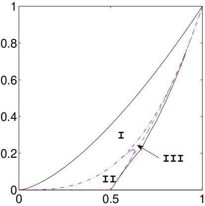
Within the parameter space $\{(\epsilon,\tau)\}\subset[0,1]^{2}$, for $1/2\leq\epsilon<1$ the lowest possible triangle density $\tau$ lies above the parabola $\tau=\epsilon(2\epsilon-1)$, except for $\epsilon_{k}=(k-1)/k,\ k\geq 2$ when $\tau_{k}$ lies on the parabola and is uniquely achieved by the complete balanced $k$-partite graph. It is convenient to add two more points to the above sequence $\{(\epsilon_{k},\tau_{k})\}$, namely $(\epsilon_{1},\tau_{1})=(0,0)$ corresponding to the empty graph, and $(\epsilon_{\infty},\tau_{\infty})=(1,1)$ corresponding to the complete graph. Furthermore, for $\epsilon$ satisfying $\epsilon_{k-1}<\epsilon<\epsilon_{k},\ k\geq 1$, the lowest possible triangle density $\tau$ lies on a known curve (a ‘scallop’), and the optimal graphs have a known structure [Ra, PR, RS1, RS2]. For all $0<\epsilon<1$ the maximization of triangle density $\tau$ for given $\epsilon$ is simpler than the above minimization: the maximum lies on $\tau=\epsilon^{3/2}$ and is uniquely achieved by a clique on enough vertices to give the appropriate value of $\epsilon$. So extremal graph theory has determined the shape of the achievable part of the parameter space as the region $R$ in Fig. 1, and determined the structure of the graphs with densities on the boundary.

Our goal is to extend the study to the interior of $R$ in a limited sense: for $(\epsilon,\tau)$ in the interior we wish to determine, asymptotically in the size of the graph, what most graphs are (or what a typical graph is) with these densities. (We clarify ‘most’ and ‘typical’ below.) The typical graph associated with $(\epsilon,\tau)$ will be described by probabilities of edges between, and within, a finite number of vertex sets, parameters which vary smoothly in $(\epsilon,\tau)$ except across phase transition curves. Phases are the maximal connected regions in which the parameters vary smoothly. One transition curve was determined in [RS2], namely $(\epsilon,\tau)=(\epsilon,\epsilon^{3}),\ 0\leq\epsilon\leq 1$. On this curve the typical graph corresponds to edges chosen independently with probability $\epsilon$. This (‘Erdös-Rényi’ or ‘ER’) curve separates $R$ into a high $\tau$ region, a single phase, and a low $\tau$ region consisting of infinitely many phases, at least one related to each scallop. We will present simulation evidence for our determination of the typical graphs of the high $\tau$ phase (phase I) and for the two phases, II and III, which are associated with the first scallop; see Fig. 2.

$\tau$

$\epsilon$

Figure 2: Boundary of phases I, II and III in the phase space. The blue dash-dotted line in the middle is the ER curve, the lower boundary of phase I.

There are two key features of these results: that by use of probability one can capture the structure of most $(\epsilon,\tau)$-constrained graphs uniquely; and that their structure is remarkably simple, for instance requiring at most four parameters for over $95\%$ of the phase space.

We conclude this section with some notation which we use to clarify our use above of the terms ‘most’ and ‘typical’ graphs.

Consider simple graphs $G$ with vertex set $V(G)$ of (labeled) vertices, edge set $E(G)$ and triangle set $T(G)$, with cardinality $|V(G)|=n$. Our main tool is $\displaystyle Z^{n,\alpha}_{\epsilon,\tau}$, the number of graphs with densities:

$$e(G)\equiv\frac{|E(G)|}{{n\choose 2}}\in(\epsilon-\alpha,\epsilon+\alpha);\quad t(G)\equiv{\frac{|T(G)|}{{n\choose 3}}}\in(\tau-\alpha,\tau+\alpha).$$ (1)

From this we define the entropy density, the exponential rate of growth of $Z^{n,\alpha}_{e,t}$ as a function of $n$. First consider

$$s^{n,\alpha}_{\epsilon,\tau}={\ln(Z^{n,\alpha}_{\epsilon,\tau})\over n^{2}},\hbox{ and then }s(\epsilon,\tau)=\lim_{\alpha\downarrow 0}\lim_{n\to\infty}s^{n,\alpha}_{\epsilon,\tau}.$$ (2)

The double limit defining the entropy density $s(\epsilon,\tau)$ was proven to exist in [RS1]. The objects of interest for us are the qualitative features of $s(\epsilon,\tau)$ in the interior of $R$. To analyze them we make use of a variational characterization of $s(\epsilon,\tau)$.

Let us first introduce some notation. Assume our vertex set $V$ is decomposed into $M$ subsets: $V_{1},\ldots,V_{M}$. We consider (probabilistic) ‘multipodal graphs’ $G_{A}$ described by matrices $A=\{A_{ij}\,|\,i,j=1,\ldots,M\}$ such that there is probability $A_{ij}$ of an edge between any $v_{i}\in V_{i}$ and any $v_{j}\in V_{j}$. Special cases in which each $A_{ij}\in\{0,1\}$ allow one to include nonprobabilistic graphs in this setting.

This setting has been further generalized to analyze limits of graphs as $n\to\infty$. (This work was recently developed in [LS1, LS2, BCLSV, BCL, LS3]; see also the recent book [Lov].) The (symmetric) matrices $A_{ij}$ are replaced by symmetric, measurable functions $g:(x,y)\in[0,1]^{2}\to g(x,y)\in[0,1]$; the former are recovered by using a partition of $[0,1]$ into consecutive subintervals to represent the partition of $V$ into $V_{1},\ldots,V_{M}$. The functions $g$ are called graphons, and using them the following was proven in [RS1] (adapting a proof in [CV]):

Variational Principle. For any possible pair $(\epsilon,\tau)$, $s(\epsilon,\tau)=\max[-I(g)]$, where the maximum is over all graphons $g$ with $e(g)=\epsilon$ and $t(g)=\tau$, where

$$e(g)=\int_{[0,1]^{2}}g(x,y)\,dxdy,\qquad t(g)=\int_{[0,1]^{3}}g(x,y)g(y,z)g(z,x)\,dxdydz$$ (3)

and the rate function is

$$I(g)=\int_{[0,1]^{2}}I_{0}[g(x,y)]\,dxdy,$$ (4)

with the function $I_{0}(u)={1\over 2}\left[u\ln(u)+(1-u)\ln(1-u)\right]$. The existence of a maximizing graphon $g=g_{\epsilon,\tau}$ for any $(\epsilon,\tau)$ was proven in [RS1], again adapting a proof in [CV].

We want to consider two graphs equivalent if they are obtained from one another by relabelling the vertices. There is a generalized version of this for graphons, with the relabelling replaced by measure-preserving maps of $[0,1]$ into itself [Lov]. The equivalence classes of graphons are called reduced graphons, and on this space there is a natural ‘cut metric’ [Lov].

We can now clarify the notions of ‘most’ and ‘typical’ in the introduction: if $g_{\epsilon,\tau}$ is the only reduced graphon maximizing $s(\epsilon,\tau)$, then as the number $n$ of vertices diverges and $\alpha_{n}\to 0$, exponentially most graphs with densities $e(G)\in(\epsilon-\alpha_{n},\epsilon+\alpha_{n})$ and $t(G)\in(\tau-\alpha_{n},\tau+\alpha_{n})$ will have reduced graphon close to $g_{\epsilon,\tau}$ [RS1].

2 Numerical Computation

To perform the study we outlined in the previous section, we combine numerical computation with local analysis. Let us first introduce our computational framework.

We need to solve the following constrained minimization problem:

$$\min_{g}I(g)$$ (5)

subject to the constraints

$$e(g)=\epsilon,\quad\mbox{and}\quad t(g)=\tau,$$ (6)

where the functionals $I(g)$, $e(g)$ and $t(g)$ are defined in  (4) and (3).

To solve this minimization problem numerically, we need to represent the continuous functions with discrete values. We restrict ourselves to the class of piecewise constant functions.

For each integer $N\geq 1$ let $P_{N}:0=p_{0}<p_{1}<p_{2}<\cdots<p_{N}=1$ be a partition of the interval $[0,1]$. We denote by $c_{i}=p_{i}-p_{i-1}$ ($1\leq i\leq N$) the sizes of the subintervals in the partition. Then we can form a partition of the square $[0,1]^{2}$ using the (Cartesian) product $P_{N}\times P_{N}$. We define the class, $G(P_{N})$, of those symmetric functions $g:[0,1]^{2}\to[0,1]$ which are piecewise constant on the subsets $P_{N}\times P_{N}$, and introduce the notation:

$$g(x,y)=g_{ij},\ \ (x,y)\in(p_{i-1},p_{i})\times(p_{j-1},p_{j}),\quad 1\leq i,j\leq N,$$ (7)

with $g_{ij}=g_{ji}$. They are probabilistic generalizations of multipartite graphs, which we call multipodal ​​: bipodal for $N=2$, tripodal for $N=3$, etc. We will call such a multipodal graphon ‘symmetric’ if all $c_{j}$ are equal and all $g_{jj}$ are equal, and otherwise ‘asymmetric’.

It is easy to check that with this type of $g$, the functionals $I$, $e$ and $t$ become respectively

$$I(g)=\displaystyle\sum_{1\leq i,j\leq N}I_{0}(g_{ij})c_{i}c_{j}=\dfrac{1}{2}\displaystyle\sum_{1\leq i,j\leq N}[g_{ij}\ln g_{ij}+(1-g_{ij})\ln(1-g_{ij})]c_{i}c_{j},$$ (8)

$$e(g)=\displaystyle\sum_{1\leq i,j\leq N}g_{ij}c_{i}c_{j},\qquad t(g)=\displaystyle\sum_{1\leq i,j,k\leq N}g_{ij}g_{jk}g_{ki}c_{i}c_{j}c_{k}.$$ (9)

Using the fact that $\cup_{N}G(P_{N})$ is dense in the space of graphons, our objective is to solve the minimization problem in $G(P_{N})$, for all $N$:

$$\min_{\{c_{j}\}_{1\leq j\leq N},\{g_{ij}\}_{1\leq i,j\leq N}}I(g),$$ (10)

with the constraints (6) and

$$0\leq g_{ij},c_{j}\leq 1,\qquad\displaystyle\sum_{1\leq j\leq N}c_{j}=1,\qquad\mbox{and}\qquad g_{ij}=g_{ji}$$ (11)

for any given pair of $\epsilon$ and $\tau$ values.

Minimum without the $\epsilon$ and $\tau$ constraints.

Let us first look at the minimization problem without the $e(g)=\epsilon$ and $t(g)=\tau$ constraints. In this case, we can easily calculate the first-order variations of the objective function:

$$I_{g_{ij}}=I_{0}^{\prime}(g_{ij})c_{i}c_{j}=\dfrac{1}{2}\ln[g_{ij}/(1-g_{ij})]c_{i}c_{j},$$ (12)

$$I_{c_{p}}=\sum_{1\leq i,j\leq N}I_{0}(g_{ij})(\dfrac{\partial c_{i}}{\partial c_{p}}c_{j}+c_{i}\dfrac{\partial c_{j}}{\partial c_{p}}),\ \ \mbox{with}\ \ \sum_{1\leq j\leq N}\dfrac{\partial c_{j}}{\partial c_{p}}=0.$$ (13)

where we used the constraint $\sum_{1\leq j\leq N}c_{j}=1$ to get the last equation.

We observe from (12) that when no constraint is imposed, the minimum of $I(g)$ is located at the constant graphon with $g_{ij}=1/2$, $1\leq i,j\leq N$. The value of the minimum is $-(\ln 2)/2=-0.34657359027997$. At the minimum, $\epsilon=1/2$ and $\tau=1/8$ (on the ER curve $\tau=\epsilon^{3}$). We can check also from (13) that indeed $I_{c_{p}}=0$ at the minimum for arbitrary partition $\{c_{j}\}$ that satisfies $\sum_{1\leq j\leq N}c_{j}=1$. This is obvious since the graphon is constant and thus the partition does not play a role here.

The second-order variation can be calculated as well:

$$I_{g_{ij}g_{lm}}=I_{0}^{\prime\prime}(g_{ij})c_{i}c_{j}\delta_{il}\delta_{jm}=\dfrac{1}{2}\frac{c_{i}c_{j}}{g_{ij}(1-g_{ij})}\delta_{il}\delta_{jm}.$$ (14)

$$I_{g_{ij}c_{p}}=I_{c_{p}g_{ij}}=I_{0}^{\prime}(g_{ij})(\dfrac{\partial c_{i}}{\partial c_{p}}c_{j}+c_{i}\dfrac{\partial c_{j}}{\partial c_{p}}),\ \ \mbox{with}\ \ \sum_{1\leq i\leq N}\dfrac{\partial c_{i}}{\partial c_{p}}=0.$$ (15)

$$I_{c_{p}c_{q}}=\sum_{1\leq i,j\leq N}I_{0}(g_{ij})\Big{(}\dfrac{\partial^{2}c_{i}}{\partial c_{p}c_{q}}c_{j}+\dfrac{\partial c_{i}}{\partial c_{p}}\dfrac{\partial c_{j}}{\partial c_{q}}+\frac{\partial c_{i}}{\partial c_{q}}\dfrac{\partial c_{j}}{\partial c_{p}}+c_{i}\dfrac{\partial^{2}c_{j}}{\partial c_{p}c_{q}}\Big{)},\\ \mbox{with}\ \ \sum_{1\leq i\leq N}\dfrac{\partial c_{i}}{\partial c_{p}}=0,\ \ \sum_{1\leq i\leq N}\dfrac{\partial^{2}c_{i}}{\partial c_{p}c_{q}}=0.$$ (16)

Thus the unconstrained minimizer is stable with respect to perturbation in $g$ values since the second variation $I_{g_{ij}g_{lm}}$ is positive definite. At the minimizer, however, the second variation with respect to $c$ is zero! This is consistent with what we know already.

We now propose two different algorithms to solve the constrained minimization problem. The first algorithm is based on Monte Carlo sampling while the second algorithm is a variant of Newton’s method for nonlinear minimization. All the numerical results we present later are obtained with the sampling algorithm and confirmed with the Newton’s algorithm; see more discussion in Section 2.3.

2.1 Sampling Algorithm

In the sampling algorithm, we construct random samples of values of $I$ in the parameter space. We then take the minimum of the sampled values. The algorithm works as follows.

• Set the number $N$ and the number of samples to be constructed ($L$); Set counter $\ell=1$;

• Generate the sizes of the blocks: $\{c_{j}^{\ell}\}\in[0,1]^{N}$ and normalize so that $\sum_{j}c_{j}^{\ell}=1$;

• Generate a sample $\{g_{ij}^{\ell}\}\in[0,1]^{N\times N}$ with $g_{ij}^{\ell}=g_{ji}^{\ell}$, $1\leq i,j\leq N$ and rescale such that:

  • $\displaystyle\sum_{1\leq i,j\leq N}g_{ij}^{\ell}c_{i}^{\ell}c_{j}^{\ell}=\epsilon$;

  • $\displaystyle\sum_{1\leq i,j,k\leq N}^{\ell}g_{ij}g_{jk}^{\ell}g_{ki}^{\ell}c_{i}^{\ell}c_{j}^{\ell}c_{k}^{\ell}=\tau$;

• Evaluate $I_{\ell}=\displaystyle\sum_{1\leq i,j\leq N}I_{0}(g_{ij}^{\ell})c_{i}^{\ell}c_{j}^{\ell}$;

• Set $\ell=\ell+1$; Go back to [1] if $\ell\leq L$;

• Evaluate $I_{N}=\min\{I_{\ell}\}_{\ell=1}^{L}$.

We consider two versions of Step [2] which work equally well (beside a slight difference in computational cost) in practice. In the first version, we generate a sample $\{g_{ij}^{\ell}\}\in[0,1]^{N\times N}$ with $g_{ij}^{\ell}=g_{ji}^{\ell}$, $1\leq i,j\leq N$. We then rescale the sample using the relation $g_{ij}^{\ell}=\gamma g_{ij}^{\ell}+\tilde{\gamma}$. The relations [A] and [B] then give two equations for the parameter $\gamma$ and $\tilde{\gamma}$. We solve the equations for $\gamma$ and $\tilde{\gamma}$. If at least one of $\{g_{ij}^{\ell}\}$ violate the condition $g_{ij}^{\ell}\in[0,1]$ after rescaling, we re-generate a sample and repeat the process until we find a sample that satisfies $g_{ij}^{\ell}\in[0,1]$ ($1\leq i,j\leq N$) after rescaling. In the second version, we simply find a sample $\{g_{ij}^{\ell}\}$ by solving [A] and [B] as a third-order algebraic system using a multivariate root-finding algorithm, with the constraint that $\{g_{ij}^{\ell}\}\in[0,1]^{N\times N}$. When multiple roots are found, we take them as different qualified samples.

This sampling algorithm is a global method in the sense that the algorithm will find a good approximation to the global minimum of the functional $I$ when sufficient samples are constructed. The algorithm will not be trapped in a local minimum. The algorithm is computationally expensive. However, it can be parallelized in a straightforward way. We will discuss the issues of accuracy and computational cost in Section 2.3.

2.2 SQP Algorithm

The second algorithm we used to solve the minimization problem is a sequential quadratic programming (SQP) method for constrained optimization. To briefly describe the algorithm, let us denote the unknown by $x=(c_{1},\cdots,c_{N},g_{11},\cdots,g_{1N},g_{21},\cdots,g_{2N},\cdots,g_{N1},\cdots,g_{NN})$. Following [GMSW], we rewrite the optimization problem as

$$\min_{x\in[0,1]^{N+N^{2}}}I(x),\quad\mbox{subject to}\quad l\leq r(x)\leq u,\qquad r(x)=\left(\begin{array}[]{c}x\\ \mathcal{A}x\\ \mathcal{C}(x)\end{array}\right)$$ (17)

where $l$ and $u$ are the lower and upper bounds of $r(x)$ respectively, $\mathcal{C}_{1}(x)=e(x)$ and $\mathcal{C}_{2}(x)=t(x)$. The matrix $\mathcal{A}$ is used to represent the last two linear constraints in (11):

$$\mathcal{A}=\left(\begin{array}[]{cc}\Sigma&{\mathbf{0}}_{1\times N^{2}}\\ {\mathbf{0}}_{N^{2}\times N}&\mathcal{S}\end{array}\right)$$ (18)

where $\Sigma=(1,\cdots,1)\in\mathbb{R}^{1\times N}$ is used to represent the constraint $\sum c_{j}=1$, ${\mathbf{0}}_{1\times N^{2}}\in\mathbb{R}^{1\times N^{2}}$ is a matrix with all zero elements, and $\mathcal{S}\in\mathbb{R}^{N^{2}\times N^{2}}$ is a matrix used to represent the symmetry constraint $g_{ij}=g_{ji}$. The elements of $\mathcal{S}$ are given as follows. For any index $k$, we define the conjugate index $k^{\prime}$ as $k^{\prime}=(r-1)N+q$ with $q$ and $r$ the unique integers such that $k=(q-1)N+r$ ($0\leq r<N$). Then for all $1\leq k\leq N^{2}$, $\mathcal{S}_{kk}=-\mathcal{S}_{kk^{\prime}}=1$ if $k\neq(j-1)N+1$ for some $j$, and $\mathcal{S}_{kk}=0$ if $k\neq(j-1)N+1$ for some $j$. All other elements of $\mathcal{S}$ are zero.

The SQP algorithm is characterized by the following iteration

$$x_{\ell+1}=x_{\ell}+\alpha_{\ell}p_{\ell},\qquad\ell\geq 0$$ (19)

where $p_{\ell}$ is the search direction of the algorithm at step $\ell$ and $\alpha_{\ell}$ is the step length. The search direction $p_{\ell}$ in SQP is obtained by solving the following constrained quadratic problem

$$\min I(x_{\ell})+\mathfrak{g}(x_{\ell})^{\mathfrak{T}}p_{\ell}+\frac{1}{2}p_{\ell}^{\mathfrak{T}}H_{\ell}p_{\ell},\qquad\mbox{subject to}\qquad l\leq r(x_{\ell})+J(x_{\ell})p_{\ell}\leq u.$$ (20)

Here $\mathfrak{g}(x_{\ell})=\nabla_{x}I$, whose components are given analytically in (12) and (13), $J(x_{\ell})=\nabla_{x}r(x_{\ell})$, whose components are given by

$$e_{g_{ij}} = c_{i}^{\ell}c_{j}^{\ell},$$ (21)

$$t_{g_{ij}} = 3\displaystyle\sum_{1\leq k\leq N}g_{jk}^{\ell}g_{ki}^{\ell}c_{i}^{\ell}c_{j}^{\ell}c_{k}^{\ell},$$ (22)

$$e_{c_{p}} = \sum_{1\leq i,j\leq N}g_{ij}^{\ell}\Big{(}\dfrac{\partial c_{i}^{\ell}}{\partial c_{p}^{\ell}}c_{j}^{\ell}+c_{i}^{\ell}\dfrac{\partial c_{j}^{\ell}}{\partial c_{p}^{\ell}}\Big{)},\ \ \mbox{with}\ \ \sum_{1\leq i\leq N}\dfrac{\partial c_{i}^{\ell}}{\partial c_{p}^{\ell}}=0$$ (23)

$$t_{c_{p}} = \displaystyle\sum_{1\leq i,j,k\leq N}g_{ij}^{\ell}g_{jk}^{\ell}g_{ki}^{\ell}\Big{(}\dfrac{\partial c_{i}^{\ell}}{\partial c_{p}^{\ell}}c_{j}^{\ell}c_{k}^{\ell}+\dfrac{\partial c_{j}^{\ell}}{\partial c_{p}^{\ell}}c_{i}^{\ell}c_{k}^{\ell}+\dfrac{\partial c_{k}^{\ell}}{\partial c_{p}^{\ell}}c_{i}^{\ell}c_{j}^{\ell}\Big{)}.$$ (24)

$H(x_{\ell})$ is a positive-definite quasi-Newton approximation to the Hessian of the objective function. We take the BFGS updating rule to form $H(x_{\ell})$ starting from the identity matrix at the initial step [NW].

We implemented the SQP minimization algorithm using the software package given in [GMSW] which we benchmarked with the fmincon package in MATLAB R2012b.

2.3 Computational Strategy

The objective of our calculation is to minimize the rate function $I$ for a fixed $(\epsilon,\tau)$ pair over the space of all graphons. Our computational strategy is to first minimize for $g\in G(P_{N})$, for a fixed number of blocks $N$, and then minimize over the number of blocks. Let $I_{N}$ be the minimum achieved by the graphon $g_{N}\in G(P_{N})$, then the minimum of the original problem is $I=\min_{N}\{I_{N}\}$. Due to limitations on computational power we can only solve up to $N=16$. The algorithms, however, are not limited by this.

By construction we know that $I_{2}\geq I_{3}\geq\cdots\geq I_{N}$. What is surprising is that our computation suggests that the minimum is always achieved with bipodal graphons in the phases that we are considering. In other words, $I_{2}=\min\{I_{N}\}_{N=2}^{N=16}$.

To find the minimizers of $I_{N}$ for a fixed $N$, we run both the sampling algorithm and the SQP algorithm. We observe that both algorithms give the same results (to precision $10^{-6}$) in all cases we have simulated. In the sampling algorithm, we observe from (12) and  (13) that the changes in $I$ caused by perturbations in $g_{ij}$ and $c_{p}$ are given respectively by $\delta I/\delta g_{ij}\sim\ln[\delta g_{ij}/(1-\delta g_{ij})]c_{i}c_{j}$ and $\delta I/\delta c_{p}\sim I_{0}(g_{ij})\delta c_{p}$. These mean that to get an accuracy of order $\eta$, our samples have to cover a grid of parameters with mesh size $\delta g_{ij}\sim{e^{{2\eta}/{c_{i}c_{j}}}}/{(1+e^{{2\eta}/{c_{i}c_{j}}})}\sim 1$ in the $g_{ij}$ direction and $\delta c_{p}\sim{\eta}/{I_{0}(g_{ij})}$ in the $c_{p}$ direction. Since $I_{0}(g_{ij})\in[-(\ln 2)/2,0]$, we have $\eta/I_{0}(g_{ij})>\eta$. It is thus enough to sample on a grid of size $\eta$. Similar analysis following  (21),  (22),  (23) and  (24) shows that, to achieve an accuracy $\eta$ on the $\epsilon$ and $\tau$ constraints, we need to sample on grids of size at most on the order of $\eta$ in both the $g_{ij}$ and $c_{p}$ directions. The total computational complexity is thus $\sim(1/\eta)^{N+N^{2}}$ in terms of function evaluations.

To run the SQP algorithm, for each $(\epsilon,\tau)$ constraint, we start from a collection of $L_{c}^{N}\times L_{g}^{N^{2}}$ initial guesses. These initial guesses are generated on the uniform grid of $L_{c}$ intervals in each $c_{p}$ direction and $L_{g}$ intervals in each $g_{ij}$ direction. They are then rescaled linearly (if necessary) to satisfy the $\epsilon$ and $\tau$ constraints. The results of the algorithm after convergence are collected to be compared with the sampling algorithm. We observe that in most cases, the algorithm converges to identical results starting from different initial guesses.

Finally we note that there are not many parameters we need to tune to get the results that we need. We observe that the SQP algorithm is very robust using the general default algorithmic parameters. The only parameters that we can adjust are $L_{c}$ and $L_{g}$ which control how many initial guesses we want to run. Our calculation shows that $L_{c}=L_{g}=10$ is enough for all the cases we studied. When we increased $L_{c}$ and $L_{g}$ to get more initial guesses, we did not gain any new minimizers.

2.4 Benchmarking the Computations

Before using the computational algorithms to explore the regions of the phase space that we plan to explore, we first benchmark our codes by reproducing some theoretically known results.

On the upper boundary.

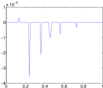
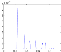
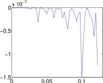
We first reproduce minimizing graphons on the curve $\tau=\epsilon^{\frac{3}{2}}$. It is known [RS2] that the minimizing graphons are equivalent to the bipodal graphon with $c=\sqrt{\epsilon}$, $g_{11}=1$ and $g_{12}=g_{21}=g_{22}=0$. The minimum value of the rate function is $I=0$. In Fig. 3 we show the difference between the simulated minimizing graphons and the true minimizing graphons given by the theory. We observe that the difference is always well below $10^{-6}$ for all the results on the curve.

$\epsilon$                                $\epsilon$                                $\epsilon$                                $\epsilon$

Figure 3: Difference between numerically computed (with superscript $num$) and true (with superscript $true$) minimizing graphons on the curve $\tau=\epsilon^{\frac{3}{2}}$. From left to right: $c^{true}-c^{num}$, $g_{11}^{true}-g_{11}^{num}$, $g_{22}^{true}-g_{22}^{num}$ and $g_{12}^{true}-g_{12}^{num}$.

On the segment $(\epsilon,\tau)=(0,0.5)\times\{0\}$.

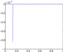
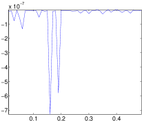
It is known that on the segment $(\epsilon,\tau)=(0,0.5)\times\{0\}$ the minimizing graphons are symmetric bipodal with $g_{11}=g_{22}=0$ and $g_{12}=g_{21}=2\epsilon$.

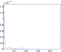
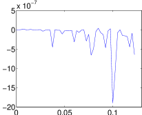
In Fig. 4 we show the difference between the simulated minimizing graphons and the true minimizing graphons given by the theory [RS2]. The differences are again very small, $<10^{-6}$. This shows again that our numerical computations are fairly accurate.

$\epsilon$                                $\epsilon$                                $\epsilon$                                $\epsilon$

Figure 4: Difference between numerically computed (with superscript $num$) and true (with superscript $true$) minimizing graphons on the line segment $(\epsilon,\tau)=(0,0.5)\times\{0\}$. From left to right: $c^{true}-c^{num}$, $g_{11}^{true}-g_{11}^{num}$, $g_{22}^{true}-g_{22}^{num}$ and $g_{12}^{true}-g_{12}^{num}$.

On the segment $(\epsilon,\tau)=\{0.5\}\times(0,0.5^{3})$.

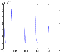
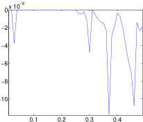
It is again known from the theory in [RS2] that on this segment the minimizing graphons are symmetric bipodal with $g_{11}=g_{22}=0.5-(0.5^{3}-\tau)$ and $g_{12}=g_{21}=0.5+(0.5^{3}-\tau)$. In Fig. 5 we show the difference between the simulated minimizing graphons and the true minimizing graphons.

$\tau$                                $\tau$                                $\tau$                                $\tau$

Figure 5: Difference between numerically computed (with superscript $num$) and true (with superscript $true$) minimizing graphons on the line segment $(\epsilon,\tau)=\{0.5\}\times(0,0.5^{3})$. From left to right: $c^{true}-c^{num}$, $g_{11}^{true}-g_{11}^{num}$, $g_{22}^{true}-g_{22}^{num}$ and $g_{12}^{true}-g_{12}^{num}$.

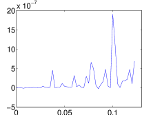
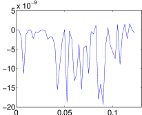
The last point on this segment is $(0.5,0.125)$. This is the point where the global minimum of the rate function is achieved. Our algorithms produce a minimizer that gives the value $I=-0.34657359$ which is less than $10^{-8}$ away from the true minimum value of $-(\ln 2)/2$.

Symmetric bipodal graphons.

In Section 3.3 we find a formula for the optimizing graphons for phase II, namely the following symmetric bipodal graphons:

$$g(x,y)=\begin{cases}\epsilon-(\epsilon^{3}-\tau)^{1/3}&x,y<1/2\hbox{ or }x,y>1/2\cr\epsilon+(\epsilon^{3}-\tau)^{1/3}&x<\frac{1}{2}<y\hbox{ or }y<\frac{1}{2}<x\end{cases}$$ (25)

Our computational algorithms also find these minimizing symmetric bipodal graphons; see discussions in the next section.

2.5 Numerical Experiments

$\tau$

$\epsilon$

Figure 6: The minimal value of $I$ at different $(\epsilon,\tau)$ values.

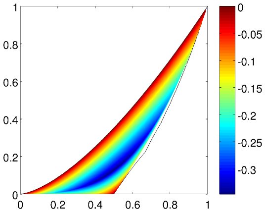
We now present numerical explorations of the minimizing graphons in some subregions of the phase space. We focus on two main subregions. The first is the subregion above the ER curve and below the upper boundary $\tau=\epsilon^{3/2}$. This is the phase I in Fig. 2. The second subregion is the region below the ER curve and above the lower boundary of the region where bipodal graphons exist. We further split this region into two separate phases, II and III; see Fig. 2. Phase II is the region where the minimizing graphons are symmetric bipodal while in phase III asymmetric bipodal graphons are the minimizers.

Figure 7: Cross-sections of the minimal value of the rate function $I$ as a function of $\tau$ along lines $\epsilon=a_{k}$ ($k=1,\cdots,10$).

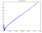
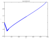
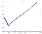
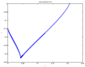
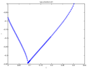
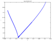
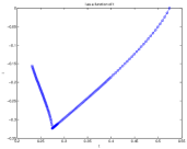
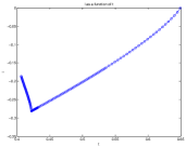
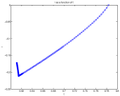
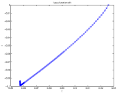
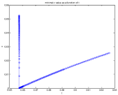
We first show in Fig. 6 the minimal values of $I$ in the whole region in which we are interested: ${\rm I\cup II\cup III}$. The minimum of $I$ for fixed $\epsilon$ is achieved on the ER curve. The cross-sections in Fig. 7 along the lines $\epsilon=a_{k}=(k-1)*0.1+0.05$ give a better visualization of the landscape of the $I$.

The main feature of the computational results is that the minimal values of the rate function $I$ in the region we show in Fig. 6 are achieved by bipodal graphons. In other words, the minimizing graphons in the whole subregion are bipodal ​​. On the ER curve, the graphons are constant. Thus the partition does not matter anymore. We consider them as bipodal purely from the continuity perspective. We show in Fig. 8 minimizing graphons at some typical points in the phase space.

Figure 8: Minimizing graphons at $\epsilon=0.3$ (left column), $\epsilon=0.6$ (middle column) and $\epsilon=0.8$ (right column). For each column $\tau$ values decrease from top to bottom. The second row represents points just above the ER curve, the third row points on the ER curve, and the fourth row points just below the ER curve. The exact $\tau$ values are given in Section 2.5.

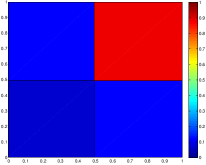
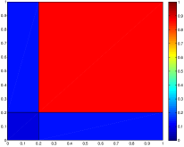
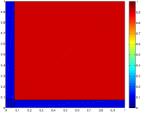
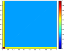
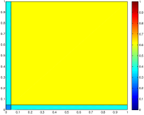
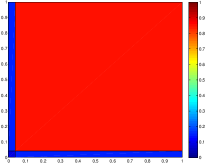
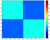
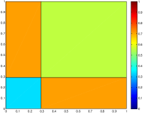
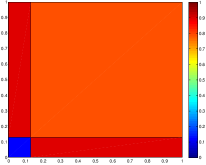
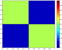
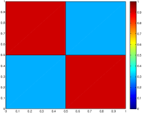
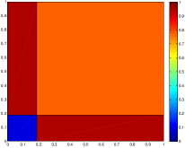
Shown are minimizing graphons at $\epsilon=0.3$ (left column), $\epsilon=0.6$ (middle column) and $\epsilon=0.8$ (right column) respectively. For the $\epsilon=0.3$ (resp. $\epsilon=0.6$ and $\epsilon=0.8$) column, the $\tau$ values for the corresponding graphons from top to bottom are $\tau=0.09565838$ (resp. $\tau=0.34037900$ and $\tau=0.61784171$) which is in the middle of phase I, $\tau=0.03070755$ (resp. $\tau=0.22010451$ and $\tau=0.55677919$) which is just above the ER curve, $\tau=0.02700000$ (resp. $\tau=0.21600000$ and $\tau=0.51200000$) which is on the ER curve, $\tau=0.02646000$ (resp. $\tau=0.21472000$ and $\tau=0.51104000$) which is just below the ER curve, and $\tau=0.01296000$ (resp. $\tau=0.18400000$ and $\tau=0.50800000$) which is in the middle of phase II (resp. phase II and phase III) respectively.

$\tau$

$\epsilon$

Figure 9: The minimal $c$ values of the minimizing bipodal graphons as a function of $(\epsilon,\tau)$.

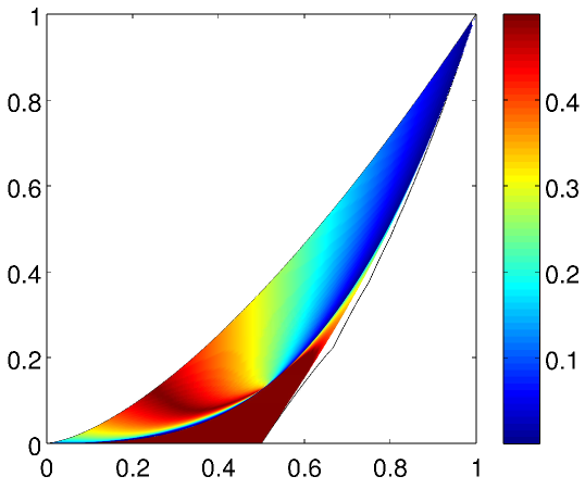
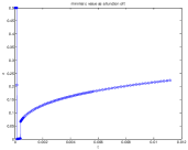
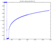
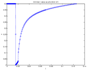
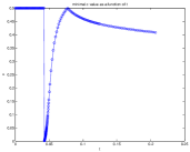
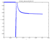
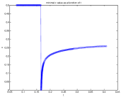
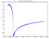
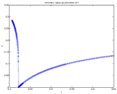
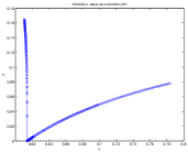
A glance at the graphons in Fig. 8 gives the impression that the minimizing graphons are very different at different values of $(\epsilon,\tau)$. A prominent feature is that the sizes of the two blocks vary dramatically. Since there is only one parameter that controls the sizes of the blocks, that is, if the first block has size $c_{1}=c$ then the second block has size $c_{2}=1-c$, we can easily visualize the change of the sizes of the two blocks in the minimizing graphons in the phase space through $c$, the size of the smaller block as a function of $(\epsilon,\tau)$. We show in Fig. 9 the minimal c values associated with the minimizing bipodal graphons. The cross-sections along the lines $\epsilon=a_{k}$ ($k=1,\cdots,10$) are shown in Fig. 10.

Figure 10: Cross-sections of the function $c(\epsilon,\tau)$ along lines of $\epsilon=0.05$, $\epsilon=0.15$, $\cdots$, $\epsilon=0.95$. The 4th and 5th graphs display coordinate singularities as the size of a cluster passes through 0.5, since we have chosen $c$ to always be 0.5 or less. The right-most kinks in those graphs are not phase transitions.

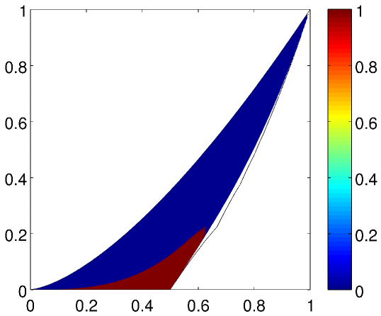
Among the minimizing bipodal graphons some are symmetric and the others are asymmetric. We show in Fig. 11 the region where the minimizing bipodal graphons are symmetric (brown) and the region where they are asymmetric (blue). This is done by checking the conditions $c_{1}=c_{2}=0.5$ and $g_{11}=g_{22}$ (both with accuracy up to $10^{-7}$) for symmetric bipodal graphons. Our numerical computation here agrees with the theoretical results we obtain later in Section 3.3.

$\tau$

$\epsilon$

Figure 11: The regions of symmetric bipodal and asymmetric bipodal optima.

3 Local Analysis

In this section we do a perturbative analysis of all three phases near the ER curve. This gives a qualitative explanation for why these three phases appear in the form they do, and we compute exactly the boundary between phases II and III, assuming the multipodal structure of the phases.

3.1 General Considerations

We treat the graphon $g(x,y)$ as the integral kernel of an operator on $L^{2}([0,1])$. Let $|\phi_{1}\rangle\in L^{2}([0,1])$ be the constant function $\phi_{1}(x)=1$. Then the edge density is $e(g)=\epsilon=\langle\phi_{1}|g|\phi_{1}\rangle$ and the triangle density is $t(g)=\tau=Tr(g^{3})$. On the ER curve the optimal graphon is $g_{0}=\epsilon|\phi_{1}\rangle\langle\phi_{1}|$. Near the ER curve we take $g=g_{0}+\delta g$, where $\langle\phi_{1}|\delta g|\phi_{1}\rangle=0$. For fixed $\epsilon$, the rate function is minimized at the ER curve, where $\tau=\epsilon^{3}$. For nearby values of $t(g)=\tau=\epsilon^{3}+\delta\tau$, minimizing the rate function involves solving two simpler optimization problems:

1. We want to minimize the size of $\delta g$, as measured in the $L^{2}$ norm, for a given $\delta\tau$.

2. We want to choose the form of $\delta g$ that minimizes $\delta I$ for a given $\|\delta g\|^{2}_{L^{2}}=\iint\delta g(x,y)^{2}\,dxdy$.

If we could solve both optimization problems simultaneously, we would have a rigorously derived optimum graphon. This is indeed what happens when $\epsilon=1/2$ and $\tau<\epsilon^{3}$ [RS2]. For other values of $(\epsilon,\tau)$, the solutions to the two optimizations disagree somewhat. In phases I and III, the actual best graphon appears to be a compromise between the two optima, while in phase II it appears to be a solution to the first optimization problem, but of a form suggested by the second problem.

By playing the two problems off of one another, we derive candidates for the optimal graphon and gain insight into the numerical results. By measuring the extent to which these candidates fail to solve each problem, we can derive rigorous estimates on the behavior of the entropy. However, we do not claim to prove that our bipodal ansatz is correct.

A simple expansion of $g^{3}=(g_{0}+\delta g)^{3}$ shows that

$$\delta\tau=3\epsilon\langle\phi_{1}|\delta g^{2}|\phi_{1}\rangle+Tr(\delta g^{3}).$$ (26)

The first term is positive-definite, while the second is indefinite.

For $\delta\tau$ negative, the solution to the first optimization problem is to have $\delta g=\nu|\psi\rangle\langle\psi|$, where $\psi$ is an arbitrary normalized vector in $L^{2}([0,1])$ such that $\langle\phi_{1}|\psi\rangle=0$. This eliminates the positive-definite term and makes the indefinite term as negative as possible, namely equal to $\nu^{3}$.

For $\delta\tau$ positive, the solution to the first optimization problem is of the form

$$\delta g=\frac{\mu}{\sqrt{2}}|\psi\rangle\langle\phi_{1}|+\frac{\mu}{\sqrt{2}}|\phi_{1}\rangle\langle\psi|+\nu|\psi\rangle\langle\psi|,$$ (27)

with $\langle\phi_{1}|\psi\rangle=0$. We then have

$$\|\delta g\|_{L^{2}}^{2}=\mu^{2}+\nu^{2};\qquad\delta\tau=\nu^{3}+\frac{3\mu^{2}}{2}(\epsilon+\nu).$$ (28)

Maximizing $\delta\tau$ for fixed $\mu^{2}+\nu^{2}$ is then a Lagrange multiplier problem in two variables with one constraint. There are minima for $\delta\tau$ at $\mu=0$ and maxima at $\nu=\mu^{2}/(2\epsilon)$.

Note that the form of the vector $\psi$ did not enter into this calculation. The form of $\psi$ is determined entirely from considerations of $\delta I$ versus $\|\delta g\|_{L^{2}}$. We now turn to this part of the problem.

The rate function $I_{0}(u)$ is an even function of $u-{1}/{2}$. Furthermore, all even derivatives of this function at $u={1}/{2}$ are positive, so the function can be written as a power series $I_{0}(u)=-{(\ln 2)}/{2}+\sum_{n=1}^{\infty}c_{n}\left(u-{1}/{2}\right)^{2n}$, where the coefficients $c_{n}$ are all positive. As a function of $(u-{1}/{2})^{2}$, $I_{0}(u)$ is then concave up. Thus the way to minimize $I(g)=\iint I[g(x,y)]\,dxdy$ for fixed $\iint\left(g(x,y)-\frac{1}{2}\right)^{2}\,dxdy$ is to have $\left[g(x,y)-{1}/{2}\right]^{2}$ constant; in other words to have $g(x,y)$ only take on two values, and for those values to sum to 1.

This is exactly our second minimization problem. We have a fixed value of $\|\delta g\|_{L^{2}}^{2}$, and hence a fixed value of

$$\iint\left(g(x,y)-\frac{1}{2}\right)^{2}\,dxdy = \iint\left(\epsilon-\frac{1}{2}+\delta g(x,y)\right)^{2}\,dxdy$$ (29)

$$= \left(\epsilon-\frac{1}{2}\right)^{2}+2\left(\epsilon-\frac{1}{2}\right)\iint\delta g(x,y)\,dxdy+\iint\delta g(x,y)^{2}\,dxdy$$ (30)

$$= \left(\epsilon-\frac{1}{2}\right)^{2}+\|\delta g\|_{L^{2}}^{2}.$$ (31)

In order for $g(x,y)$ to only take on two values, we need $\psi$ to only take on two values. After doing a measure-preserving transformation of $[0,1]$, we can assume that

$$\psi(x)=\psi_{c}(x):=\begin{cases}\sqrt{\frac{1-c}{c}}&x<c\cr&\cr-\sqrt{\frac{\phantom{1}c\phantom{1}}{1-c}}&x>c\end{cases}$$ (32)

for some constant $c\leq\frac{1}{2}$.

We henceforth restrict our attention to the ansatz (27) with the function (32), and vary the parameters $\mu$, $\nu$ and $c$ to minimize $I(g)$ while preserving the fixed values of $\epsilon$ and $\tau$.

3.2 Phase I: $\tau>\epsilon^{3}$

Suppose that $\tau$ is slightly greater than $\epsilon^{3}$. By our previous analysis, we want $\delta g$ to be small in an $L^{2}$ sense. Maximizing $\delta\tau$ for fixed $\|\delta g\|_{L^{2}}$ means taking $\nu={\mu^{2}}/{(2\epsilon)}\ll\mu$, so

$$\delta\tau=\frac{3\mu^{2}\epsilon}{2}+\frac{3\mu^{4}}{4}+\frac{\mu^{6}}{8\epsilon^{3}};\qquad\|\delta g\|_{L^{2}}^{2}=\mu^{2}+\frac{\mu^{4}}{4\epsilon^{2}}.$$ (33)

If $\epsilon\neq 1/2$, then there is no way to make $\left|g(x,y)-{1}/{2}\right|$ constant while keeping $\delta g$ pointwise small. Instead, we take $\delta g(x,y)$ to be large in a small region. We compute

$$g(x,y)=\begin{cases}\epsilon-\mu\sqrt{2}\sqrt{\frac{\phantom{1}c\phantom{1}}{1-c}}+\nu\frac{1}{1-c}&x,y>c\cr\epsilon+\frac{\mu}{\sqrt{2}}\left(\sqrt{\frac{1-c}{c}}-\sqrt{\frac{\phantom{1}c\phantom{1}}{1-c}}\right)-\nu&x<c<y\hbox{ or }y<c<x\cr\epsilon+\mu\sqrt{2}\sqrt{\frac{1-c}{c}}+\nu\frac{1-c}{c}&x,y<c\end{cases}$$ (34)

By taking $c={\mu^{2}}/{2(2\epsilon-1)^{2}}+O(\mu^{4})$, we can get the values of $g$ in the rectangles $x<c<y$ (or $y<c<x$) and the large square $x,y>c$ to sum to 1. This makes $I_{0}[g(x,y)]$ constant except on a small square of area $c^{2}=O(\mu^{4})$. Since $g(x,y)$ is equal to $\epsilon-{\mu^{2}}/{(1-2\epsilon)}+O(\mu^{4})$ when $x,y>c$, we have

$$I(g) = I_{0}\left(\epsilon-\frac{\mu^{2}}{1-2\epsilon}\right)+O(\mu^{4})$$ (35)

$$= I_{0}(\epsilon)-I_{0}^{\prime}(\epsilon)\frac{\mu^{2}}{1-2\epsilon}+O(\mu^{4})$$ (36)

$$= I_{0}(\epsilon)-\frac{2I_{0}^{\prime}(\epsilon)\delta\tau}{3\epsilon(1-2\epsilon)}+O(\delta t^{2})$$ (37)

Thus

$$\frac{\partial s(\epsilon,\tau)}{\partial\tau}=\frac{\ln\left(\frac{\epsilon}{1-\epsilon}\right)}{3\epsilon(1-2\epsilon)}+O(\delta\tau)$$ (38)

just above the ER curve.

This ansatz gives an accurate description of our minimizing graphons near the ER curve, and these extend continuously all the way to the upper boundary $\tau=\epsilon^{3/2}$. Although the behavior in a first-order neighborhood of the ER curve changes discontinuously when $\epsilon$ passes through 1/2, the behavior a finite distance above the ER curve appears to be analytic in $\epsilon$ and $\tau$, so that the entire region between the ER curve and the upper boundary corresponds to a single phase. As can be seen from these formulas, or from the numerics of Section 2, phase I has the following qualitative features:

1. The minimizing graphon is bipodal ​​. The smallest value of $g(x,y)$ is found on one of the two square regions $x,y<c$ or $x,y>c$, and the largest value is found on the other, with the value on the rectangles $x<c<y$ and $y<c<x$ being intermediate.

2. If $\epsilon\neq 1/2$, then as $\tau$ approaches $\epsilon^{3}$ from above, $c$ goes to 0. The value of $g(x,y)$ is then approximately $\epsilon$ on the large square $x,y>c$ and $1-\epsilon$ on the rectangles. If $1/3<\epsilon<2/3$, then the value of $g(x,y)$ on the small square $x,y<c$ is approximately $2-3\epsilon$; the value is close to 1 if $\epsilon<1/3$ and close to zero if $\epsilon>2/3$.

3. Conversely, as $\tau$ moves away from $\epsilon^{3}$, $c$ grows quickly, to first order in $\delta\tau$. When $\epsilon<1/2$, the small-$c$ region is quite narrow, as one sees in the second row of Fig. 8, and is easy to miss with numerical experiments. Although rapid, the transition from small-$c$ to large-$c$ appears to be continuous and smooth, with no sign of any phase transitions.

4. As $\tau$ approaches $\epsilon^{3/2}$ (from below, of course), the value of $g(x,y)$ approaches 1 on a square of size $\sqrt{\epsilon}$, approaches zero relatively slowly on the rectangles, and approaches zero more quickly on the other square. In a graph represented by such a graphon, there is a cluster representing a fraction $\sqrt{\epsilon}$ of the vertices. The probability of two vertices within the cluster being connected is close to 1, the probability of a vertex inside the cluster being connected to a vertex outside the cluster is small, and the probability of two vertices outside the cluster being connected is very small.

3.3 Phases II and III: $\tau<\epsilon^{3}$

When $\tau<\epsilon^{3}$, we want to minimize the $\mu^{2}$ term in $\delta\tau$ and make the $\nu^{3}$ term as negative as possible. This is done by simply taking $\mu=0$ and $\nu=(\delta\tau)^{1/3}$. This gives a graphon of the form

$$g(x,y)=\begin{cases}\epsilon+\nu\frac{1-c}{c}&x,y<c\cr\epsilon-\nu&x<c<y\hbox{ or }y<c<x\cr\epsilon+\nu\frac{\phantom{1}c\phantom{1}}{1-c}&x,y>c\end{cases}$$ (39)

which is displayed in the left of Fig. 12.

Figure 12: The graphons for the expressions in  (39) (left),  (40) (middle) and  (41) (right) respectively.

Note that $\nu$ is negative, so the value of the graphon is less than $\epsilon$ on the squares and greater than $\epsilon$ on the rectangles. The two vertex clusters of fraction $c$ and $1-c$ prefer to connect with each other than with themselves.

When $c\neq 1/2$, this gives a graphon that takes on 3 different values. When $c=1/2$, the graphon takes on only two values, but these values do not sum to 1. Only when $\epsilon=c=1/2$ can we simultaneously solve both optimization problems.

To understand which problem “wins” the competition, we look at the situation when $\epsilon<1/2$ and $\tau$ is slightly less than $\epsilon^{3}$. In this region, the entropy cost for having $\mu\neq 0$ is lower order in $\epsilon^{3}-\tau$ than the entropy cost for violating the second problem. This shows that the optimal bipodal graphon must have $c$ close to $1/2$, validating the use of perturbation theory around $c=1/2$.

In subsection 3.4, we compute the second variation of the rate function with respect to $c$ at $c=1/2$, and see that it is positive for all values of $\tau<\epsilon^{3}$ when $\epsilon<1/2$, and for some values of $\tau$ when $1/2<\epsilon<0.629497839$. In this regime, the best we can do is to pick $c=1/2$ and $\mu$ exactly zero. Our graphon then takes the form

$$g(x,y)=\begin{cases}\epsilon-(\epsilon^{3}-\tau)^{1/3}&x,y<1/2\hbox{ or }x,y>1/2\cr\epsilon+(\epsilon^{3}-\tau)^{1/3}&x<\frac{1}{2}<y\hbox{ or }y<\frac{1}{2}<x\end{cases}$$ (40)

These symmetric bipodal graphons, displayed in the middle of Fig. 12, are the optimizers for phase II.

The symmetric bipodal phase II has a natural boundary. If $\epsilon>1/2$, then the smallest possible value of $\tau$ is when $\nu=\epsilon-1$, in which case $\tau=2\epsilon^{3}-3\epsilon^{2}+3\epsilon-1$. It is possible to get lower values of $\tau$ with $c\neq 1/2$, and still lower values if the graphon is not bipodal ​​. Thus there must be a phase transition between phase II and the asymmetric bipodal phase III.

Phase III has its own natural boundary. Among bipodal graphons, the minimum triangle density for a given edge density (with $\epsilon>1/2$) is given by a graphon of the form

$$g(x,y)=\begin{cases}0&x,y<c\cr 1&x<c<y\hbox{ or }y<x<c\cr\alpha&x,y>c\end{cases}$$ (41)

displayed in the right of Fig. 12, where $c,\alpha\in[0,1]$ are free parameters.

The edge and triangle densities are then

$$\epsilon=2c(1-c)+(1-c)^{2}\alpha;\qquad\tau=(1-c)^{3}\alpha^{3}+3c(1-c)^{2}\alpha.$$ (42)

Minimizing $\tau$ for fixed $\epsilon$ yields a sixth order polynomial equation in $c$, which we can solve numerically.

The main qualitative features of phases II and III are

1. The minimizing graphon consists of two squares, of side $c$ and $1-c$, and two $c\times(1-c)$ rectangular regions. The value of the graphon is largest in the rectangular regions and smaller in the squares. In phase II we have $c=1/2$, and the value of the graphon is the same in both squares. In phase III we have $c<1/2$, and the value of the graphon is smallest in the $c\times c$ square.

2. All points with $\epsilon<1/2$ and $\tau<\epsilon^{3}$ lie in phase II. As $\tau\to 0$, the graphon describes graphs that are close to being bipartite​​, with two clusters of equal size such that edges within a cluster appear with probability close to zero, and edges between clusters appear with probability close to $2\epsilon$.

3. When $\epsilon>1/2$, phase II does not extend to its natural boundary. There comes a point where one can reduce the rate function by making $c$ less than 1/2. For instance, when $\epsilon=0.6$ one can construct symmetric bipodal graphons with any value of $\tau$ between $2\epsilon^{3}-3\epsilon^{2}+3\epsilon-1=0.152$ and $\epsilon^{3}=0.216$. However, phase II only extends between $\tau=0.152704753$ and $\tau=0.20651775$, with the remaining intervals being phase III. The actual boundary of phase II is computed in the next subsection.

4. Phase III, by constrast, appears to extend all the way to its natural boundary, shown in Fig. 2, to the current numerical resolution in the $\tau$ variable. The union of phases I, II, and III appears to be all values of $(\epsilon,\tau)$ that can be achieved with a bipodal graphon.

5. When we cross the natural boundary of phase III, the larger of the two clusters breaks into two equal-sized pieces, with slightly different probabilities of having edges within and between those sub-clusters. The resulting tripodal graphons have $g(x,y)$ strictly between 0 and 1, and (for $\epsilon<2/3$) extend continuously down to the $k=3$ scallop.

6. Throughout phases I, II, and III, there appears to be a unique graphon that minimizes the rate function. We conjecture that this is true for all $(\epsilon,\tau)$, and that the minimizing graphon for each $(\epsilon,\tau)$ is $k$-podal with $k$ as small as possible.

3.4 The boundary between phase II and phase III

In both phase II and phase III, we can express our graphons in the form (27). For each value of $c$ we can vary $\mu$ and $\nu$ to minimize the rate function, while preserving the constraint on $\tau$. Let $\mu(c)$ and $\nu(c)$ be the values of $\mu$ and $\nu$ that achieve this minimum for fixed $c$. Note that changing $c$ to $1-c$ and changing $\mu$ to $-\mu$ results in the same graphon, up to reparametrization of $[0,1]$. By this symmetry, $\mu(c)$ must be an odd function of $c-{1}/{2}$ while $\nu(c)$ must be an even function.

Since $\tau=\epsilon^{3}+\nu^{3}+3(\epsilon+\nu)\mu^{2}/2$ is independent of $c$, we obtain constraints on derivatives of $\mu(c)$ and $\nu(c)$ by computing

$$0=\tau^{\prime}(c) = 3\nu^{2}\nu^{\prime}+\frac{3\mu^{2}\nu^{\prime}}{2}+3(\epsilon+\nu)\mu\mu^{\prime}$$ (43)

$$0=\tau^{\prime\prime}(c) = 6\nu(\nu^{\prime})^{2}+3\nu^{2}\nu^{\prime\prime}+\frac{3\mu^{2}\nu^{\prime\prime}}{2}+6\mu\mu^{\prime}\nu^{\prime}+3(\epsilon+\nu)(\mu^{\prime})^{2}+3(\epsilon+\nu)\mu\mu^{\prime\prime},$$ (44)

where ^′ denotes $d/dc$. Since $\mu(1/2)=0$, the first equation implies that $\nu^{\prime}(1/2)=0$, while the second implies that

$$\nu^{\prime\prime}=-\frac{\epsilon+\nu}{\nu^{2}}(\mu^{\prime})^{2}$$ (45)

at $c=1/2$.

We next compute the rate function. We expand the formula (27) as

$$g(x,y)=\begin{cases}\epsilon+\nu\frac{1-c}{c}+\mu\sqrt{2}\sqrt{\frac{1-c}{c}}&x,y<c\cr\epsilon-\nu+\frac{\mu}{\sqrt{2}}\left(\sqrt{\frac{1-c}{c}}-\sqrt{\frac{\phantom{1}c\phantom{1}}{1-c}}\right)&x<c<y\hbox{ or }y<c<x\cr\epsilon+\nu\frac{c}{1-c}-\mu\sqrt{2}\sqrt{\frac{\phantom{1}c\phantom{1}}{1-c}}&x,y<c.\end{cases}$$ (46)

This makes the rate function

$$I(g) = c^{2}I_{0}\left(\epsilon+\nu\frac{1-c}{c}+\sqrt{2}\mu\sqrt{\frac{1-c}{c}}\right)$$ (49)

$$+2c(1-c)I_{0}\left(\epsilon-\nu+\frac{\mu}{\sqrt{2}}\left(\sqrt{\frac{1-c}{c}}-\sqrt{\frac{\phantom{1}c\phantom{1}}{1-c}}\right)\right)$$

$$+(1-c)^{2}I_{0}\left(\epsilon+\nu\frac{c}{1-c}-\mu\sqrt{2}\sqrt{\frac{c}{1-c}}\right)$$

Taking derivatives at $c=1/2$ and plugging in (45) yields

$$\left.\frac{d^{2}I}{dc^{2}}\right|_{c=1/2}=A(\mu^{\prime})^{2}+B\mu^{\prime}+C,$$ (50)

where

$$A = I_{0}^{\prime\prime}(\epsilon+\nu)+\frac{(\epsilon+\nu)[I_{0}^{\prime}(\epsilon-\nu)-I_{0}^{\prime}(\epsilon+\nu)]}{2\nu^{2}}$$ (51)

$$B = 2\sqrt{2}\left[I_{0}^{\prime}(\epsilon+\nu)-I_{0}^{\prime}(\epsilon-\nu)-2\nu I_{0}^{\prime\prime}(\epsilon+\nu)\right]$$ (52)

$$C = 4[I_{0}(\epsilon+\nu)-2\nu I_{0}^{\prime}(\epsilon+\nu)+2\nu^{2}I_{0}^{\prime\prime}(\epsilon+\nu)-I_{0}(\epsilon-\nu)],$$ (53)

and $\nu=-(\epsilon^{3}-\tau)^{1/3}$. The actual value of $\mu^{\prime}$ is the one that minimizes this quadratic expression, namely $\mu^{\prime}=-B/(2A)$. At this value of $\mu^{\prime}$, $d^{2}I/dc^{2}$ equals ${(4AC-B^{2})}/{(4A)}$. As long as the discriminant $B^{2}-4AC$ is negative, $d^{2}I/dc^{2}>0$ and the phase II graphon is stable against changes in $c$. When $B^{2}-4AC$ goes positive, the phase II graphon becomes unstable and the minimizing graphon has $c$ different from $1/2$.

Since the function $I_{0}$ is transcendental, it is presumably impossible to express the solution to $B^{2}-4AC=0$ in closed form. However, it is easy to compute this boundary numerically, as shown in Fig. 2.

4 Exponential Random Graph Models

There is a large, rapidly growing literature on the analysis of large graphs, much of it devoted to the analysis of some specific large graph of particular interest; see [N] and the references therein. There is also a significant fraction of the literature which deals with the asymptotics of graphs $g$ as the vertex number diverges (see [Lov]), and in these works a popular tool is ‘exponential random graph models’ (‘ERGMS’) in which a few densities $t_{j}(g),\ j=1,2,\ldots$, such as edge and triangle densities, are selected, conjugate parameters $\beta_{j}$ are introduced, and the family of relative probability densities:

$$\rho_{\beta_{1},\beta_{2},\ldots}=\exp[{n^{2}(\beta_{1}t_{1}(g)+\beta_{2}t_{2}(g)+\ldots)}]$$ (54)

is implemented on the space $G(n)$ of all simple graphs $g$ on $n$ vertices. Densities are assumed normalized to have value 1 in the complete graph, so the analysis is relevant to ‘dense graphs’, which have order $n^{2}$ edges.

$\rho_{\beta_{1},\beta_{2},\ldots}$ has the obvious form of a grandcanonical ensemble, with free energy density

$$\psi_{\beta_{1},\beta_{2},\ldots}={1\over n^{2}}\ln\Big{[}\sum_{g\in G(n)}\exp[{n^{2}(\beta_{1}t_{1}(g)+\beta_{2}t_{2}(g)+\ldots)}]\Big{]}$$ (55)

and suggests the introduction of other ensembles. This paper is the third in a sequence in which we have studied dense networks in the microcanonical ensemble, in this paper specializing to edge and triangle densities.

One goal in the study of the asymptotics of graphs is emergent phenomena. The prototypical emergent phenomena are the thermodynamic phases (and phase transitions) which ‘emerge’ as volume diverges in the statistical mechanics of particles interacting through short range forces. The results motivated by these – the mathematics of phase transitions in large dense graphs [CD, RY, AR, LZ, RS1, Y, RS2, YRF] – are a significant instance of emergence within mathematics. We conclude with some observations on the relationship between the phase transitions in dense networks as they appear in different ensembles.

In the statistical mechanics of particles with short range forces there is a well-developed theory of the equivalence of ensembles, and in particular any phase transition seen in one ensemble automatically appears in any other ensemble because corresponding free energies are Legendre transforms of one another and transitions are represented by singularies in free energies [Ru]. For particles with long range forces (mean-field models) the equivalence of ensembles can break down [TET]. For dense networks this is known to be the case [RS1]. So the precise relationship between the phase decomposition in the various ensembles of dense networks is an open problem of importance. For instance in ERGMS one of the key results is a transition within a single phase, structurally similar to a gas/liquid transition, whose optimal graphons are all Erdös-Rényi [CD, RY]. This phenomenon does not seem to have an obvious image in the microcanonical ensemble of this paper, but this should be explored.

Another important open problem is the phase structure associated with the remaining scallops.

References

- [AR] D. Aristoff and C. Radin, Emergent structures in large networks, J. Appl. Probab. 50 (2013) 883-888.
- [BCL] C. Borgs, J. Chayes and L. Lovász, Moments of two-variable functions and the uniqueness of graph limits, Geom. Funct. Anal. 19 (2010) 1597-1619.
- [BCLSV] C. Borgs, J. Chayes, L. Lovász, V.T. Sós and K. Vesztergombi, Convergent graph sequences I: subgraph frequencies, metric properties, and testing, Adv. Math. 219 (2008) 1801-1851.
- [CD] S. Chatterjee and P. Diaconis, Estimating and understanding exponential random graph models, Ann. Statist. 41 (2013) 2428-2461.
- [CV] S. Chatterjee and S.R.S. Varadhan, The large deviation principle for the Erdős-Rényi random graph, Eur. J. Comb. 32 (2011) 1000-1017.
- [GMSW] P.E. Gill, W. Murray, M.A. Saunders and M.H. Wright, User’s guide for NPSOL 5.0: A Fortran package for nonlinear programming, Technical Report SOL 86-6, System Optimization Laboratory, Stanford University, 2001.
- [Lov] L. Lovász, Large networks and graph limits, American Mathematical Society, Providence, 2012.
- [LS1] L. Lovász and B. Szegedy, Limits of dense graph sequences, J. Combin. Theory Ser. B 98 (2006) 933-957.
- [LS2] L. Lovász and B. Szegedy, Szemerédi’s lemma for the analyst, GAFA 17 (2007) 252-270.
- [LS3] L. Lovász and B. Szegedy, Finitely forcible graphons, J. Combin. Theory Ser. B 101 (2011) 269-301.
- [LZ] E. Lubetzky and Y. Zhao, On replica symmetry of large deviations in random graphs, Random Structures and Algorithms (to appear), arXiv:1210.7013 (2012).
- [N] M.E.J. Newman, Networks: an Introduction, Oxford University Press, 2010.
- [NW] J. Nocedal and S.J. Wright, Numerical Optimization, Springer-Verlag, New York, 1999.
- [PR] O. Pikhurko and A. Razborov, Asymptotic structure of graphs with the minimum number of triangles, arXiv:1203.4393 (2012).
- [Ra] A. Razborov, On the minimal density of triangles in graphs, Combin. Probab. Comput. 17 (2008) 603-618.
- [RS1] C. Radin and L. Sadun, Phase transitions in a complex network, J. Phys. A: Math. Theor. 46 (2013) 305002.
- [RS2] C. Radin and L. Sadun, Singularities in the entropy of asymptotically large simple graphs, arXiv:1302.3531 (2013).
- [Ru] D. Ruelle Statistical Mechanics; Rigorous Results, Benjamin, New York, 1969.
- [RY] C. Radin and M. Yin, Phase transitions in exponential random graphs, Ann. Appl. Probab. 23 (2013) 2458-2471.
- [TET] H. Touchette, R.S. Ellis and B. Turkington, Physica A 340 (2004) 138-146.
- [Y] M. Yin, Critical phenomena in exponential random graphs, J. Stat. Phys. 153 (2013) 1008-1021.
- [YRF] M. Yin, A. Rinaldo and S. Fadnavis, Asymptotic quantization of exponential random graphs, arXiv:1311.1738 (2013).