Green’s functions from real-time bold-line Monte Carlo
Abstract
We present two methods for computing two-time correlation functions or Green’s functions from real time bold-line continuous time quantum Monte Carlo. One method is a formally exact generalized auxiliary lead formalism by which spectral properties may be obtained from single-time observables. The other involves the evaluation of diagrams contributing to two-time observables directly on the Keldysh contour. Additionally, we provide a detailed description of the bold-line Monte Carlo method. Our methods are general and numerically exact, and able to reliably resolve high-energy features such as band edges. We compare the spectral functions obtained from real time methods to analytically continued spectral functions obtained from imaginary time Monte Carlo, thus probing the limits of analytic continuation.
I Introduction
Strongly correlated electron materials exhibit fascinating collective behavior which has long challenged our understanding.Dagotto (2005) A few notable examples include Mott metal–insulator transitions in transition metal oxides,Imada et al. (1998) colossal magnetoresistance in perovskite manganites,Dagotto (2003) quantum criticality in heavy fermion systemsCusters et al. (2003) and high temperature superconductivity in copper oxidesBednorz and Müller (1986) and pnictides.Kamihara et al. (2008) Of central experimental interest are dynamical properties, both of excited states near the Fermi energy and at highly excited energies. However, the theoretical description of correlated electron materials has proven difficult: because of the absence of a small parameter, perturbation theory is in general unreliable. Traditional materials science techniques, among them the density functional theory (DFT)Hohenberg and Kohn (1964); Kohn and Sham (1965) and the GW approximation,Hedin (1965) do not capture strong correlation effects, while standard numerically exact lattice methodsBlankenbecler et al. (1981); White (1992); Corboz et al. (2010) are limited to small lattices, high symmetry points or one dimensional systems.
An alternative to directly determining quantities in a correlated quantum lattice model is provided by the dynamical mean field theory (DMFT).Metzner and Vollhardt (1989); Georges and Kotliar (1992); Georges et al. (1996) In the approximation that correlations are local, the physics of the lattice model can be mapped onto a numerically tractable impurity model: a finite interacting system coupled self-consistently to a noninteracting effective bath. Extensions of DMFT systematically relax the approximation of locality.Maier et al. (2005); Toschi et al. (2007); Rubtsov et al. (2008)
In addition to their importance for dynamical mean field theory, quantum impurity models are extremely important in their own right, since they appear directly in a variety of problems including nanoscience (where they are used in describing quantum transportMeir et al. (1993)) and catalysis and surface science (where they can be used to model the adsorption of molecules on surfacesBrako and Newns (1981)). The general solution of such impurity models remains a formidable challenge. Exact solutionsTsvelick and Wiegmann (1983) are only available in specific limits.Andrei (1980); Vigman et al. (1982) A variety of more general semi-analyticalKeiter and Kimball (1970, 1971); Pruschke and Grewe (1989); Georges and Kotliar (1992); Haule et al. (2001) methods have been used successfully. Numerical approaches—all of which are general in principle, but have different advantages and limitations in practice—include the numerical renormalization group,Wilson (1975); Bauer et al. (2009) exact diagonalization,Caffarel and Krauth (1994) configuration interaction,Zgid et al. (2012) hierarchical equations of motionJin et al. (2008); Hou et al. (2013) and quantum Monte Carlo.Hirsch and Fye (1986); Rubtsov et al. (2005); Werner et al. (2006); Gull et al. (2011a)
Continuous time Monte Carlo (CTQMC) algorithmsRubtsov et al. (2005); Werner et al. (2006); Gull et al. (2011a) are numerically exact and very general in the sense that their computational complexity is independent of the spectral resolution and band shape, a property which is particularly crucial in the context of DMFT. Most algorithms are formulated on the Matsubara axis, and therefore access to single- and two-particle response functions as measured in experiments requires an analytic continuation to the real axis. This analytic continuation problem is ill-posed: small fluctuations in the (input) Matsubara data, due to Monte Carlo noise, cause large changes in the output real frequency data and render the direct inversion of the continuation kernel unreliable for practical purposes. Instead, analytical continuation algorithms perform the inversion under additional assumptions, e.g. that the function be described by a small number of zeros and poles on the complex plane,Haymaker and Schlessinger (1970) that it deviate as little as possible from a ‘default model’ function while being consistent with the input data within some predetermined error bounds,Jarrell and Gubernatis (1996) or that it be as smooth as possible.Prokof’ev and Svistunov (2013)
While analytical continuation methods produce spectral functions that are consistent with Matsubara data, the bias that they introduce on the real axis is hard to quantify and, as a consequence, controlled error estimates and confidence intervals on the real axis are not available even for numerically exact Matsubara data.
Real time methods, on the other hand, embody a controlled way to study the dynamical properties of quantum impurity models. Monte Carlo impurity solvers have also been formulated on the Keldysh contour,Mühlbacher and Rabani (2008); Werner et al. (2009); Schiró and Fabrizio (2009); Werner et al. (2010) such that analytical continuation is unnecessary (although a combination of real time and Matsubara techniques may be beneficialDirks et al. (2013)). In the weakly interacting limit, response functions at short times immediately after a quantum quench have been obtained in this way.Eckstein et al. (2009) Using the newest generation of real time impurity solvers, bold-lineProkof’ev and Svistunov (2007, 2008) CTQMC,Gull et al. (2010, 2011b) single time quantities have been obtained at substantially longer times and at large interaction strength, so that, in combination with reduced dynamics techniques,Cohen and Rabani (2011) the long time steady state behavior in the Kondo regime was reached after a quantum quench.Cohen et al. (2013a)
Here we present two ways of obtaining spectral functions from real time CT-QMC in the strong correlation limit. These methods were recently used to access nonequilibrium spectral properties;Cohen et al. (2013b) here we present the details of the methodology, focusing for clarity on the equilibrium aspects and applications. We emphasize, however, that the methods are equally applicable to nonequilibrium situations. The first method obtains real frequency spectral functions from two-time correlation functions which are then Fourier transformed. The second is based on an auxiliary current formulation, and is more efficient when one is interested in obtaining spectral steady state or equilibrium properties. This second method is compatible with the reduced dynamics technique of Ref. Cohen et al., 2013c and with any numerical solver applicable to transport. It simulates a direct measurement of the spectral function by coupling auxiliary probes to the system, and is a generalization of the concept introduced for the wide band limit by Refs. Sun and Guo, 2001; Lebanon and Schiller, 2001, which was implemented in this limit within real-time path integral Monte Carlo.Mühlbacher et al. (2011)
In Sec. II we define the class of models to which our method is applicable. In Sec. III we derive a generalized version of the auxiliary current method in the spirit of previous work, and in Sec. IV we introduce a new, fully general scheme compatible with CTQMC. In Sec. V we provide an introduction to the numerically exact real time bold-line CTQMC method; as an example, we work out the case of the Anderson impurity model, starting from strong-coupling expansion. In Sec. VI we present results obtained from an implementation of the scheme for the Anderson impurity model within bold-line CTQMC, and we explore the limitations of analytical continuation. Finally, in Sec. VII, we summarize our findings and discuss our conclusions.
II Model
We consider a general quantum impurity model described by
| (1) |
, the dot Hamiltonian, can be any (generally interacting) Hamiltonian of the form
| (2) |
with denoting dot operators. , the total number of degrees of freedom on the dot, is assumed to be small. describes on-site energy levels, the interaction represents the strength of four-operator (two-body) terms, and the ellipsis all potential higher order interactions.
The bath or lead Hamiltonian is:
| (3) | ||||
| (4) |
is written here as a sum of bath terms which may be characterized by different dispersions and different thermodynamic parameters (such as temperature and chemical potential) entering through the initial conditions. In a molecular electronics scenario with left and right leads, and the index takes the corresponding values and . has infinite degrees of freedom described by lead operators and a lead dispersion but is noninteracting.
The third term is the hybridization Hamiltonian , which describes population transfer between the dot and leads. Here we assume it to have the bilinear form
| (5) | ||||
| (6) |
characterized by a hopping from dot to lead. The coupling densities defined as , fully define the properties of bath and hybridizations for the purpose of this paper. We will assume to be diagonal in dot orbital space but allow it to differ for each lead, such that . General coupling density matrices will be discussed briefly in Sec. IV.
Information about thermodynamic parameters, e.g. the lead chemical potential or the lead temperature, is encapsulated in the initial conditions of the system. For example, fermionic leads at an inverse temperature and a chemical potential are described by an initial Fermi Dirac distribution .
III Auxiliary current method
In their seminal 1992 paper, Meir and Wingreen showed that if initial correlations can be neglected, the steady-state current out of lead can be written as:Meir and Wingreen (1992)
| (7) | ||||
Here, and are the electron charge and Planck’s constant (both are set to one from here onward); is the initial occupation of lead ; and , and are the dot’s retarded, advanced and lesser Green’s functions, respectively. The difference between the retarded and advanced Green’s function is proportional to the dot’s spectral function:
| (8) |
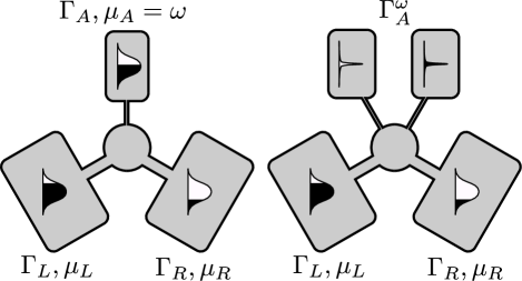
As previous authors have pointed out,Sun and Guo (2001); Lebanon and Schiller (2001) if the are independent of energy and the orbital structure of is diagonal at all frequencies such that it can be treated as a scalar (i.e. for ), then can be obtained by coupling the system to an additional auxiliary lead with index . Here we generalize this approach to the case where the are not energy independent but proportional: and (note that the next section introduces a generalized scheme where these assumptions are not required). The extended system, illustrated on the left panel of Fig. 1, is described by the following modifications to the Hamiltonian:
| (9) | ||||
| (10) | ||||
| (11) | ||||
| (12) |
with and chosen such that . The index denotes the auxiliary lead. Following Refs. Sun and Guo, 2001; Lebanon and Schiller, 2001, we use the conservation of current along with Eq. (7) and (8) to construct an expression for in which no longer appears:
| (13) | ||||
| (14) | ||||
In the limit where , system properties such as the Green’s functions are unaffected by the presence and properties of the auxiliary lead. Therefore, the derivative of the current with respect to the chemical potential in the auxiliary lead, , only contains contributions from :
| (15) | ||||
With our assumption that and are diagonal, the trace of over the impurity degrees of freedom is a product over their elements (up to a factor of , which we will ignore). If lead is maintained at low enough temperature, we can also set , which allows us to perform the integration and obtain
| (16) | ||||
| (17) |
This result is identical to the one of Refs. Sun and Guo, 2001; Lebanon and Schiller, 2001, except in that is allowed to have an arbitrary energy dependence. The approach outlined here is, in general, limited to systems with only diagonal dot correlation and hybridization functions.
Eq. (16) and (17) allow sampling the spectral function by measuring the current flow between the dot and a weakly coupled auxiliary lead at a variety of chemical potentials. This could also in principle be done in an experimental setting by varying the gate voltage of an auxiliary lead, and this is perhaps the greatest advantage of this variant of the method. However, the setup is only useful in cases where is not suppressed. Near regions where is small, must be very small in order for not to diverge, and the numerical computation or measurement of the derivative must be performed to a very high accuracy. For this reason, the presence of noise makes the numerical computation of this derivative impractical within a Monte Carlo simulation, at least for cases where one is interested in behavior in or near a gap in the lead’s spectrum.
IV Double probe scheme
In order to bypass the limitation outlined above and the need to compute derivatives, we propose an alternative scheme. The current in the auxiliary lead is (see(7))
| (18) | ||||
In the limit the partial derivative of this equation with respect to immediately yields Eq. (17) without the factor , the higher order terms of which constitute corrections in powers of . Our form ignores the secondary effects of the auxiliary lead on the currents through other leads, and only becomes accurate in the limit of an auxiliary lead that is weakly coupled to the system ( small), a criterion that can be verified a posteriori by varying . Additionally, no assumptions regarding the relationship or proportionality between and need to be made. This freedom allows the experimentally unrealistic but numerically convenient choice of introducing two auxiliary leads, one empty and one full, set up in such a way that they are coupled to the system at only a single frequency :
| (19) | |||||
| (20) |
Using these definitions, we define two auxiliary currents
| (21) | |||||
| (22) | |||||
| (23) |
The assumption made here, as in Ref. Sun and Guo, 2001; Lebanon and Schiller, 2001 and the preceding section, is that is small enough that the properties of the auxiliary lead have a negligible effect on the physical properties of the full system. We note in passing that this same idea also allows for the use of a single wide-bandwidth auxiliary lead in the case where the coupling densities are not proportional.
Two independent calculations, one for an empty lead and a second one for a full lead, provide a setup (see right side of Fig. 1) with which the dot spectral function can be obtained. Restoring physical constants for a moment,
| (24) |
This analytically exact result is not restricted to any particular way of solving the impurity model, and is therefore usable within any formalism where one has access to currents. Apart from quantum Monte Carlo this includes hierarchical equation of motion methods. Intuitively, the introduction of two leads of opposite populations simultaneously should correct current conservation to some degree (since the coupling densities are no longer proportional, an exact statement is hard to make), but they can also be connected one at a time at the price of a small loss in accuracy, as long as is taken to be small enough.
Equations Eq. (21) and Eq. (22) also provide direct access to the lesser Green’s function , providing the full information about single particle correlations even in nonequilibrium situations. Finally, since can be chosen to have any dot orbital matrix structure, it is straightforward to find a choice that allows extracting individual elements of .
Since no numerical derivative needs to be taken, the double probe scheme performs better within a Monte Carlo simulation, in addition to providing more information (such as ). Any practical implementation will need to approximate the delta function in Eq. 20 by a smooth numerical approximation. In this work, we approximate with Gaussians with an amplitude and width small enough that the results are independent of them within the numerical precision bounds and frequency resolution we need (a good rule of thumb is to start the amplitude and width at least an order of magnitude or two below any other energy scale in the problem; one then verifies convergence in both parameters of the Gaussian by systematically varying them). The picture which emerges is physically intuitive: we probe the system using a pair of virtual leads, one of which is empty of electrons while the one other is full. The leads are coupled very weakly and only within a narrow frequency range. By measuring the rate at which electrons are injected into one lead and extracted from the other, one obtains information about the average density of single-electron excitations within the frequency range probed.
The auxiliary current method by construction contains two-time information, but strictly speaking this only corresponds to the two-time correlation function in a certain adiabatic limit (where the relaxation of the auxiliary current to its final value is much faster than that of the system’s dynamical timescales). However, the method has a straightforward extension to the handling of two-time correlation functions; this can be seen by considering eq. (15) in Ref. Jauho et al., 1994, which connects the current through any lead to the two-time Green’s function by way of a generalized coupling density . By considering this expression, it is easy to see how a generalized, time-dependent auxiliary coupling density might be devised, which fully and rigorously probes the full two-time correlation functions. This is beyond the scope of the present work.
V Bold-line Monte Carlo
The auxiliary current formalism is only useful in combination with a method for computing currents through interacting quantum dots. This requires the solution of a correlated quantum many-body problem, and therefore a numerical method. Several approaches exist. In this section we present a detailed description of the real-time bold-line continuous-time hybridization expansion quantum Monte Carlo algorithm introduced in Ref. Gull et al., 2011b. We focus in particular on the observables required for obtaining two-time correlation functions but, for the sake of simplicity, limit ourselves to the single-orbital Anderson impurity model.
The method is based on a stochastic summation of all diagrams containing partially summed (‘bold’ rather than ‘bare’) propagator lines and vertex functions. So far, these partially summed propagators have come from the non-crossing or one-crossing approximations (NCA or OCACohen et al. (2013a)) but the method is more general: In a first, quasi-analytic step, an underlying diagrammatic approximation selecting some (but not all) diagrams is chosen, and propagators within that approximation are obtained analytically or via the solution of a set of coupled integral equations. In a second step, all corrections to the propagators are summed up using a stochastic Monte Carlo procedure, so that the resulting sum contains all diagrams and therefore becomes numerically exact. The precise choice of the underlying approximation determines the speed of convergence to the exact result, the statistical uncertainty, and the feasibility of the method for any given system, but has no effect on the final answer if convergence is attained. The imaginary time version of bold-line CTQMC has been introduced in Ref. Gull et al., 2010. The formulation on the Keldysh contour and the advantages of bold-line CTQMC over bare CTQMC in the non-equilibrium context have been discussed and benchmarked in Ref. Gull et al., 2011b, and an extension to OCA and to a reduced dynamics formulation has appeared in Ref. Cohen et al., 2013a.
We consider the single-orbital Anderson impurity model, where we set in Eq. (2) such that there may be up to two electrons having opposite spin indices and on the dot simultaneously. The dot Hamiltonian becomes
| (25) |
the lead Hamiltonian
| (26) |
and the dot-lead hybridization
| (27) |
We first derive a version of the bare real time hybridization expansion by introducing a perturbation theory written in terms of many-body atomic state propagators. The expectation value of an operator at time in the interaction picture with respect to is
| (28) |
Here is the initial density matrix. We assume that it can be factorized into dot and lead parts (this assumption can be relaxed by adding an imaginary branch to the contour). is the interaction picture propagator, and interaction picture operators are denoted by a subscript and given by . We then expand and in the formMahan (1990)
| (29) |
thus obtaining an infinite series of terms. It is convenient to imagine that interactions coming from exist on a forward branch while those coming are on a backward branch; the union of these two contours forms the real part of the Keldysh contour. Notably, since in our choice of model and expansion is interacting, Wick’s theorem does not hold and one cannot at this point apply standard diagrammatic tools.
The interaction form of the Hybridization term is
| (30) |
with denoting the spin opposite of . All terms of change the state of the dot by adding or removing one electron from it, while time evolution with leaves the dot state invariant. It is therefore convenient to group certain sets of contributions together in dressed () and bare ( propagators
| (31) | ||||
| (32) |
between the many-body states and on the dot, with the leads traced out. Both atomic state propagators and correlation functions are often referred to as Green’s functions (in addition, the retarded and advanced Green’s functions are often referred to as propagators), but the objects defined here differ from correlation functions in several important ways—most notably, they have an exponentially larger dimensionality, since they contain matrix elements between pairs of many-body states rather than single-particle level indices. Diagrammatically, a propagator over a segment of one branch of the Keldysh contour represents all diagrams having all their interactions contained in said segment, that begin and end with the index states.

For the Anderson model, the bare atomic state propagators (Eq. 32) are
| (33) |
The factor is independent of the dot state and factors out of all expressions; for physical quantities it is always exactly canceled by complementary contributions from the two branches of the Keldysh contour: It can therefore safely be ignored and will be neglected from here onwards.
Since the trace over the bath is zero unless the same number of creation and annihilation operators for each spin occurs, the full atomic state propagator is also diagonal for the Anderson impurity model. It can be expanded in terms of bare propagators using Eq. 29. The first non-vanishing contribution is:
| (34) | ||||
| (35) | ||||
Using Eq. 30 and Eq. 33, this can be written as
| (36) | ||||
where
| (37) | ||||
defines the hybridization function (note that spin indices have been suppressed for brevity). The hybridization function for each lead can be expressed in terms of the coupling densities of that lead and its initial occupation probability, both of which are obtained from the lattice Green’s function within DMFT. It is if appears before on the Keldysh contour, and otherwise, with
| (38) | ||||
| (39) |
This second order term contains all the elements occurring in the expansion, namely the bare propagators and hybridization lines. A graphical representation is shown in Fig. 2: in the upper left panel, atomic state propagators for a given state are represented by a pair of lines; the upper one representing spin up, the lower one spin down. Dotted lines represent empty states and solid lines represent occupied states, such that the full set of states is represented by lines. Additionally, thick (or bold) lines represent full propagators while thin lines stand for bare propagators. Full propagators are built out of all possible combinations of bare propagators and interaction vertices (shown to the upper right), with all interaction times integrated over. Every hybridization line connects two interactions, and each such line comes with the minus sign of Eq. 35. The second order contribution explicitly written above includes both the and term in the expansion of shown in the bottom part of Fig. 2, where an additional order diagram is also shown.
The essence of the CTQMC methodMühlbacher and Rabani (2008); Werner et al. (2009); Gull et al. (2011a); Rubtsov et al. (2005) is that one can evaluate the sum of all diagrams by sampling them stochastically using the Metropolis algorithm. In particular, the ‘continuous time’ descriptor implies that, unlike in previous algorithms,Hirsch and Fye (1986)systematic Trotter time-discretization errors are absent.Gull et al. (2007) In the hybridization expansion continuous-time algorithm,Werner et al. (2006); Gull et al. (2011a) the stochastic sampling of diagrams is done by insertion of pairs of dot operators and hybridization lines: Namely, in each Monte Carlo step, a hybridization line and two dot operators are created, destroyed, or moved. This set of updates can be shown to respect ergodicity, and moves can be weighed in such a way that detailed balance is also maintained.Gull et al. (2011a) Since the leads are noninteracting both initially and under propagation by , Wick’s theorem is respected for lead (though not for the dot) operators, and it is possible to efficiently sum large sets of diagrams having the same path—dot state as a function of time—in the form of determinants, significantly reducing the sign problem.Werner et al. (2006)

In bold-line CTQMC, rather than summing each diagram explicitly, one first obtains an approximation for the atomic state propagator that is better than the bare atomic state propagator by dressing it using some ansatz for the self energy. If one chooses a self-consistent approximation such as the NCA or OCA, this allows for the relatively inexpensive computation of a renormalized, or bold line, propagator which contains an infinite (though still partial) set of diagrams. This is not the full propagator, but often represents a reasonable approximation to it. It is then possible to write all additional diagrams in terms of this new bold propagator. To avoid double counting diagrams, one must take into account only diagrams which do not contain parts already summed within the underlying approximation. In a Monte Carlo algorithm this is feasible if one rejects any update that leads to an unwanted diagram, while ascertaining that still all diagrams are generated (thus maintaining ergodicity). Each diagram in the bare expansion is contained in exactly one bold diagram, which has the same number of or fewer vertices. Since the original expansion was convergent, the sampling process of all diagrams gives the same exact answer—however, if the renormalized propagators contain a large proportion of the most important contributions, convergence occurs at lower diagram order, is substantially faster, and the sign problem is greatly alleviated.Gull et al. (2011b)
The NCA approximation to the propagator is described pictorially in the first two terms of Fig. 3 with one hybridization line (see also Ref. Cohen et al., 2013a, which uses a more compact notation). The OCA also includes the two additional diagrams with two hybridization lines. The auxiliary state self energy is inserted into the causal Dyson equation
| (40) | ||||
and solved self-consistently. For Hamiltonians without an explicit time dependence, like the Anderson impurity Hamiltonian considered here, the propagator is a function of only time differences even outside of steady state conditions. This can be seen directly from its definition in Eq. 31. In terms of numerical effort the cost of solving the Dyson equation is therefore negligible even for very long propagation times, within both the NCA and the OCA.
Bold diagrams no longer have the determinant structure of bare diagrams, since some permutations of lead operators are contained in the underlying partial summation, while most are not. It is therefore necessary to explicitly treat the sum of individual hybridization lines. In practice, cancellation effects of diagrams with the same dot operator configuration but different hybridization lines are large, so that taking into account all legal hybridization line contractions of a given dot operator configuration at once, similar to computing the determinant, is preferable to sampling them individually. The cost of explicitly counting hybridization line contractions scales exponentially with diagram order (and time). In contrast, determinants can be computed at polynomial cost. However, the dynamical sign problem, which always appears in non-equilibrium Monte Carlo calculations, also incurs an exponential cost as a function of time, so that both methods are exponential. In all applications considered so far, the bold method converges at orders that are low enough that the dynamical sign problem of the bare (or bold) expansion, and not the exponential/polynomial scaling with diagram order, is the limiting factor.
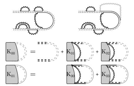
So far, we have discussed only the propagators, which exist on a single branch of the Keldysh contour. To obtain physical observables in real time, one must take into account diagrams on both branches as well as diagrams crossing branches. The structure of such inter-branch diagrams is illustrated on the top left of Fig. 4. The example shows a contribution to the probability that the dot is in the state at the final time at the right tip of the contour, while beginning in state . Inter-branch hybridization lines are a crucial part of the expansion, as they allow changes to the state at the tip.
Generalizing the Monte Carlo process to the double contour poses no difficulties greater than those entailed by the extra bookkeeping (due to the fact that vertices on the two branches contribute opposite signs, while time on the two branches flows in opposite directions). However, the dressed propagators contain no information about inter-branch diagrams. Just as one can use the bold line technique to renormalize the propagators, it is possible and highly advantageous to obtain partial summations of contour-crossing diagrams into vertex corrections. An example of a set of self-consistent equations defining a vertex correction is shown in the lower panel of Fig. 4. This particular vertex function, which we call the vertex, sums both non-crossing intra-branch and inter-branch diagrams. It gives all such contributions starting from some initial condition (marked by the left index, 0 here) at the beginning of the contour and terminating at some final condition (the right index) at a pair of propagation times, one of which is on either branch. The rest of the contour (shown in gray) can then be filled by any bold diagram not containing contributions already summed within the vertex.
The two equations shown are part of a set of four coupled integral equations which must be solved self-consistently, as they also depend on and . The final two equations have an analogous structure. There are four such sets, one for each value of the initial condition (see also Ref. Gull et al., 2011b and Ref. Cohen et al., 2013a, which used a notation that compacts all 16 -vertex equations into one equation and also includes the OCA contribution). Since the 16 elements of the vertex are two time objects, they are stored in discretized form in large matrices. Currently a uniform discretization is used and the memory requirements for the partial summation part of the method is a bottleneck of the method. All integrals within the NCA vertices and all but a few within the OCA take the form of a convolution (for a Hamiltonian with no explicit time dependence), and can be performed efficiently in Fourier space. The remaining integrals are amenable to parallelization on clusters, and current implementations scale linearly to over a thousand nodes on high-performance clusters.
Two important examples of observables which will be presented in the results below are the electronic current into the different leads and the two-time correlation function. Both observables are given by diagrams which have a special line at the end of the Keldysh contour, shown as the light gray line on the upper right corner of Fig. 4. This line is created by an operator at the final measured time. To measure the current with spin out of certain leads, the hybridization function for the special line should be replaced by the one defined by Eq. 37, with the sum over restricted to values within the chosen subset of leads (for instance, to measure the “left” current one only sums over values in the left lead). To measure two-time correlation functions, the value of the hybridization line becomes unity (as it describes free operators and which do not come with a corresponding lead operator and coupling), and the contribution is binned with respect to the location of the operator at the other end of the line. With combinations of such lines one can construct any single particle correlation function (, etc.).
As mentioned earlier, in practice all possible contractions of hybridization lines from a diagram are taken into account simultaneously; this means that the final expression for a contribution to (say) the current from any given diagram is identical to the one introduced in Eq. (62-66) of Ref. Werner et al., 2009, but with terms already accounted for by the partial resummation excluded from the evaluation of the determinant of Eq. (59) of that reference.
In using bold-line CTQMC within the context of reduced dynamics for dot observables,Cohen and Rabani (2011); Cohen et al. (2013a) the somewhat more complex observables were implemented which measure the current through one spin for a preselected occupation of the other spin. It should be clear from the description above how the generalization proceeds: one accepts only current diagrams where the opposite spin meets the desired criterion. In fact, since both possible criteria are needed for the reduced dynamics, all contributions to the single-spin current can be sampled in each Monte Carlo trajectory, as long as during the measurement only the appropriate observable for each configuration is updated. A reduced dynamics treatment which also allows for the computation of non-dot observables such as the current would require a further addition of observables to the simulation.Cohen et al. (2013c)
VI Results
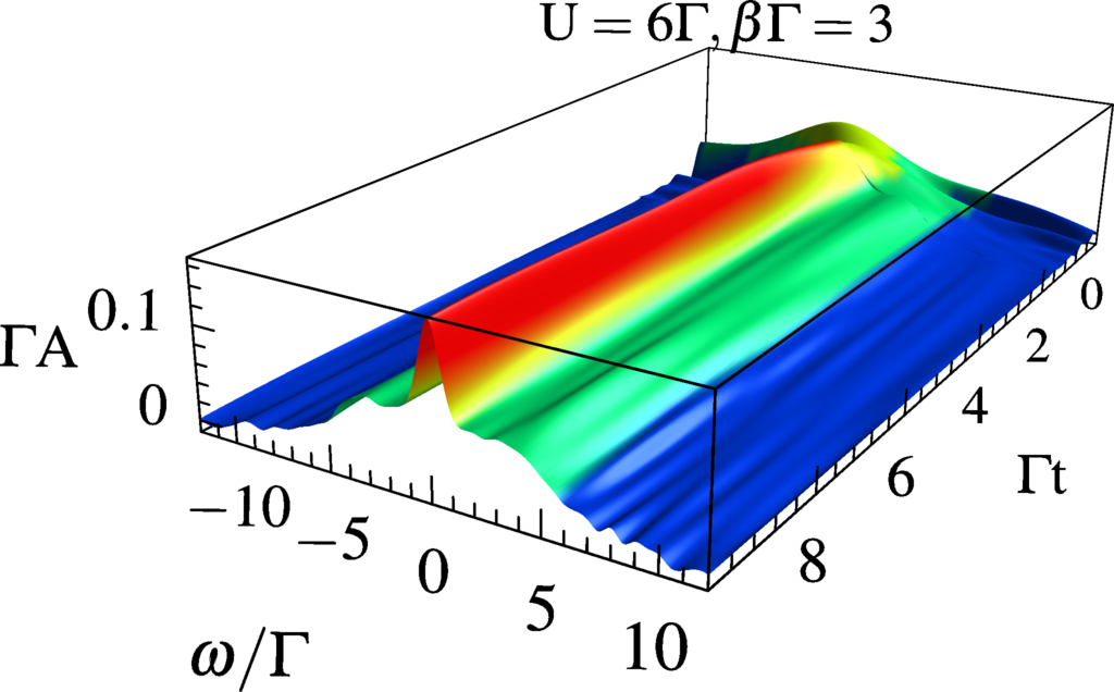
We now show results for the spectral function of the Anderson impurity model, obtained using bold-line CTQMC and the auxiliary current method and a direct measurement of the time-dependent Green’s function. To constrain the parameter space we restrict ourselves to the particle-hole symmetric case and to a single flat band with a soft cutoff . We choose and hold the lead chemical potential at 0, while varying dot interaction , the lead temperature , and the band cutoff energy . All results are computed with the real time bold-line CTQMC expansionGull et al. (2011b); Cohen et al. (2013a) built around the one-crossing approximation (OCA) Eckstein and Werner (2010) by measuring the current to an auxiliary reservoir defined by
| (41) |
with and . The dot is initially decoupled from the physical and auxiliary leads, and the coupling is turned on at time zero, after which the system time-evolves according to the full Hamiltonian, Eq. (1).
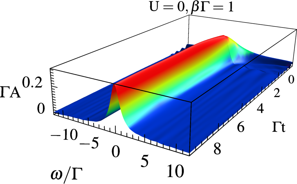
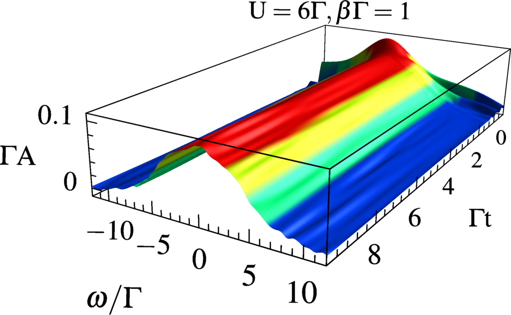
Little is known about the properties of the spectral function as measured from the auxiliary current, Eq. (24), as a function of time; what we have shown rigorously is only is that at steady state or equilibrium it must approach the spectral function known from other methods. At intermediate timescales this quantity contains information about quench dynamics (since the dot begins in an out-of-equilibrium state where it is decoupled from the bath), but the interpretation of this data must be performed with care, since the physical dynamics are mixed to some degree with those of the auxiliary lead. We therefore begin the discussion by exploring it in detail for the three examples shown in Fig. 5. The as measured by our virtual probes is plotted as a function of time. Note that a constant- cut across the surface at long times forms the steady state spectral function, which can be read from the profile of the plots. With the initial () condition we have chosen, the auxiliary current is always zero. In all three cases, the band cutoff energy of the leads is set to ; the band can therefore be considered essentially flat over the range of frequencies displayed. The long time limit corresponds to the equilibrium situation.
On the left, we display a noninteracting case. Within hybridization expansion CTQMC, the noninteracting case is a stringent test for the algorithm, as it expands about the atomic limit making this exactly solvable limit a difficult case for our approach. First, the final profile has a Lorentzian shape, as expected from a noninteracting dot coupled to a flat lead. Second, the observed relaxation timescale appears to be related to rather than the auxiliary parameters and . This is typical for charge-related properties in the system, and suggests that we are in fact measuring physical system properties and not properties related to our choice of auxiliary lead. This is expected, since the auxiliary lead is coupled to the system only weakly, so that probing the dot only involves its linear response characteristics.
The behavior at both short and long timescales can alternatively be visualized by taking cuts through this data at planes of fixed , as shown in the top panel of Fig. 6. Here, we see that relaxation to equilibrium occurs somewhat more slowly for energies near the Fermi level. At short timescales the data contains information about the nonequilibrium evolution of the system in a quench situation, but this is mixed to some degree with the relaxation properties of the auxiliary lead. Exploring the implications of this in detail is beyond the scope of the current work.
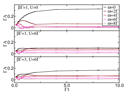
In the middle panel of Fig. 5, a strong interaction has been turned on, while the temperature is kept rather high. At long times, excitations spread throughout the band, but not far beyond . In addition, noise and oscillations in both time and frequency appear, indicating that convergence to the steady state is much slower. However, as before, the time evolution of the spectral function is mostly converged after a time on the order of (see also the corresponding middle panel of Fig. 6).
On the right side of Fig. 5 the temperature is lowered while the interaction is reduced. The formula is commonly used to estimate the Kondo temperatureHewson (1993) and gives , yet even at the predicted spectrum clearly begins to display the characteristics of Kondo physics, and one can observe the formation of a central peak at the chemical potential and an indication of two side bands. Interestingly, the time scale over which the general profile develops does not appear to be significantly modified, but long-time oscillations which have not fully attenuated by our final simulation time appear. This suggests that obtaining numerical convergence for this particular parameter set requires longer propagation times than required in the strongly interacting regime. On the other hand, it also suggests that obtaining a basic estimate of the spectral function only requires comparatively short propagation times (see also the corresponding lower panel of Fig. 6).
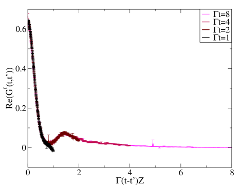
As explained in Section V, within bold-CTQMC two-time correlation functions can also be obtained directly for a given and . The result of one such evaluation for is displayed in Fig. 7. At equilibrium must become a function of the difference between its two time parameters, but for any finite it exists only for . We expect that for large enough , the correlation function measured as a function of should converge to the equilibrium value; Fig. 7 illustrates that while this clearly is not the case for , convergence occurs rather quickly. For the parameters shown, at one obtains reliable estimates of two-time correlation functions in equilibrium for any .
Once the equilibrium correlation function is obtained in the time domain, a simple Fourier transform takes us to the frequency domain, where the spectral function may be obtained using Eq. 8. In practice, since is limited in range by the maximum reachable, one must also converge the result of the Fourier transform in at all frequencies. This proves to be difficult, and we will show that when one is interested in frequency domain properties the auxiliary current method offers more accurate results. However, for certain nonequilibrium problems, it is often the time-domain function itself that proves to be of interest.Cohen et al. (2013b); Eckstein et al. (2009)
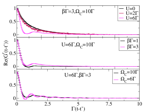
The dependence of the real part of the retarded equilibrium Green’s function on the physical parameters of the system is explored in Fig. 8. The top panel shows that while the effect of weak interaction is relatively mild, strong interaction induces qualitative changes in the structure of the correlations. The central panel shows that these effects are mitigated but not destroyed by higher temperatures. Finally, the bottom panel shows how a reduction in the bandwidth of the bath results in the introduction of high-frequency oscillations into the correlation function.
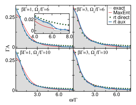
To validate our results, Fig. 9 compares the spectral function, as obtained with real time bold-line CTQMC from both the auxiliary current method and the direct Fourier transformation of the time-domain correlation function, to the exact spectrum in the noninteracting case, shown as the gray shaded region terminated by a dashed black line. We note that this is a particularly difficult limit for bold-line CTQMC based on the OCA, as OCA performs poorly for small values of ; to decrease the amount of computer time needed, we have limited the maximum order of bold diagrams to , despite the fact that higher order contributions are contributing on the order of a few percent. As a basis for assessing the accuracy of the proposed method compared to existing implementations, we also show a result obtained from a simulation of the same model using the imaginary time hybridization Monte Carlo method,Werner et al. (2006), analytically continued using the Maximum EntropyJarrell and Gubernatis (1996) algorithm (MaxEnt) with an unbiased flat default model.
Fig. 9 clearly shows that none of the numerical methods perfectly reconstruct the exact spectral function. The real time auxiliary current method (blue line with error bars denoting statistical, but not finite time or order truncation errors) is the only one to perform consistently well at all parameters and frequencies shown. However, some systematic errors remain, in particular at the band edges and near the chemical potential. The Fourier-transformed real time correlation function (green circles) is not as accurate, and in particular displays a high-frequency tail caused by numerical noise (the auxiliary lead formulation circumvents this by the finite width of the auxiliary lead’s coupling density. However, this always induces an averaging over a finite frequency window).
The MaxEnt result computed with a flat model (solid red line) in Fig. 9 appears to behave relatively well only at low temperature and large bandwidth, as seen in the bottom right panel. As we raise the temperature—going from the bottom right to the bottom left panel—MaxEnt fails, in particular at frequencies near the resonance. The peak is at odds with the bias towards flatness present in our default model, and causes a noticeable deviation from the correct result as we go from bottom right to top right panel. While the MaxEnt results are incompatible with the real time results, the back-continuation of the real-time results to the imaginary axis (where imaginary time Monte Carlo results are numerically exact) agrees perfectly with the imaginary time results, and the back-continuation of the continued MaxEnt results also agrees perfectly with the imaginary time results. The fact that two completely incompatible real-frequency spectra can have the same Matsubara frequency representation (within Monte Carlo errors on the imaginary axis) is well known and caused by the large number of very small eigenvalues of the analytic continuation kernel. Continuing further to the top left panel, when both temperature is low and bandwidth is high, MaxEnt results are unreliable both at high and at low frequencies (while, again, imaginary frequency Green’s functions agree within errors). As seen in the inset, no signature of high energy features, e.g. the band edge, is discernible. This also remains true at lower temperatures.
A few caveats regarding the comparison with MaxEnt are in order. First, analytic continuation is an ill-posed problem, and the analytically continued result depends strongly on the algorithm and parameters used. In the case of MaxEnt, it also depends on the model. As the algorithm is based on a penalty for deviations from the default model, a correct guess for the noninteracting system would have lead to the exact result. We therefore stress here that additional information (e.g. from low-order perturbation theory or high-temperature simulations) may yield substantially better results by taking advantage of additional knowledge; it may however also be a source of bias. In the context of real time method, the ill-posed continuation problem can be avoided and the sources of ambiguity introduced when continuing results to the real axis are absent from the start.
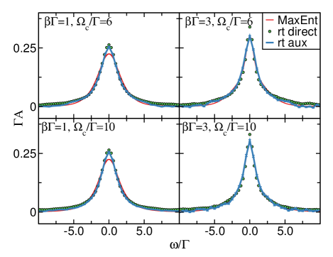
We now turn to the exploration of the results of the direct measurement of the spectral function and of the auxiliary current method in combination with bold-line CTQMC in interacting systems. In Fig. 10 we increase the interaction strength to . The two real time methods are in far better agreement in this case, but deviations at high frequency are visible. Once again, only the real time auxiliary current correctly captures the existence of a band edge, and the MaxEnt method is unable to capture the results both for low band width and high temperature.
The nonzero interaction makes convergence with the order of bold diagrams much easier to obtain, as the quality of the OCA approximation improves and the number of hybridization events decreases. Still, these weakly interacting parameters remain beyond the scope where NCA or OCA are accurate. In fact, even a perturbative weak coupling treatment would be sufficient in this regime. The main result of this plot is therefore that it highlights the ability of OCA based bold-line CTQMC to treat interacting problems substantially beyond the range where OCA itself—without Monte Carlo—is accurate.
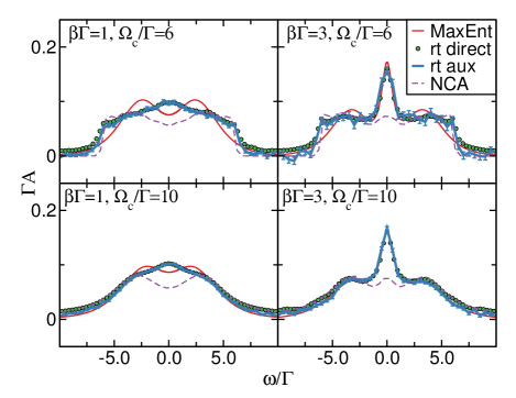
Next, we continue to a strongly interacting case, Fig. 11, with . Here is large enough that NCA can be a useful approximation, and we include it for comparison. As before, the two real time methods give consistent results at small to intermediate frequencies. At large bandwidth and low temperatures (lower right), all Monte Carlo methods, including imaginary time CTQMC, yield similar results except at high frequencies, while the NCA underestimates the height of the central resonance. However, when either the bandwidth or the temperature is varied, a dramatic change occurs: lowering the bandwidth (upper right) results in the development of a high and sharp band edge, which the MaxEnt method misses completely. In this respect, MaxEnt actually performs even worse than NCA (though results are clearly much better at low frequencies). At higher temperature (lower left of Fig. 11), both MaxEnt and NCA underestimate the central resonance, resulting in a dip where a peak should be and in a qualitatively different spectral shape at low frequencies. When both temperature and bandwidth are varied simultaneously, NCA continues to suffer from the same problem, while MaxEnt suffers from both simultaneously, resulting in a qualitatively incorrect spectral function at all frequencies.
We note that previous authors have found that at least for some parameters, a perturbative expansion including select diagrams beyond the OCA results in substantially better approximations.Eckstein and Werner (2010) Using these higher order expansions as a starting point within bold-line CTQMC is expected to improve its convergence properties further, making it potentially easier to obtain reliable, unbiased data independent of the underlying approximation.
VII Summary and conclusions
To conclude, we have proposed and implemented two methods of obtaining Green’s functions from real-time bold-line CTQMC. The first one directly evaluates two-time correlation functions, while the second one is based on a newly proposed double-probe scheme for the computation of an auxiliary current. The auxiliary current method is general enough to be used with other numerical methods, and is especially helpful when two-time correlation functions are impossible or more expensive to acquire, as is the case in formalisms relying on reduced dynamics. We compared these two methods to each other, to analytically continued data and to data obtained within the non-crossing approximation. In general the real time methods give more accurate results and the auxiliary current method in particular even resolves high-energy features such as hard band edges. Numerically exact convergence accounting for all sources of errors remains technically difficult to achieve. The MaxEnt method (in the particular variation we chose to test) does not reconstruct high-frequency features. At low temperature it performs very well at low frequencies, but at higher temperatures it fails. We demonstrate that for certain choices of model parameters, which are neither special nor extreme, both MaxEnt and NCA produce qualitatively misleading results.
Real time methods remain substantially more expensive than imaginary time methods in terms of the computer time needed to accomplish similar tasks, and will in all probability remain so. As DMFT continues to evolve towards being a general-purpose tool for material science, it is plausible to assume that better scaling methods capable of treating larger impurities with more orbitals per site will become standard, even for real-time dynamics. While in this paper we have considered only expansions about the NCA and OCA for a single-site Anderson impurity model, the ideas and formalism are general: they can also be used for other formal resummations, or for expansions about more complicated models such as those arising in cluster extensions of dynamical mean field theory. Even now, real time methods offer (aside from the ability to address nonequilibrium situations, which was discussed elsewhereCohen et al. (2013b)) an alternative and controlled route to access spectral quantities at high frequency that is not available with other tools, and will find its use in particular in real-time DMFT.
Acknowledgements.
The authors would like to thank Rainer Härtle for his useful input on many occasions. GC is grateful to the Yad Hanadiv–Rothschild Foundation for the award of a Rothschild Postdoctoral Fellowship. GC and EG acknowledge TG-DMR120085 and TG-DMR130036 for computer time. DRR acknowledges NSF CHE-1213247, AJM acknowledges NSF DMR 1006282, and EG acknowledges DOE ER 46932. This research used resources of the National Energy Research Scientific Computing Center, which is supported by the Office of Science of the U.S. Department of Energy under Contract No. DE-AC02-05CH11231. Our implementations were based on the ALPS Bauer et al. (2011) libraries.References
- Dagotto (2005) E. Dagotto, Science 309, 257 (2005).
- Imada et al. (1998) M. Imada, A. Fujimori, and Y. Tokura, Reviews of Modern Physics 70, 1039 (1998).
- Dagotto (2003) E. Dagotto, Nanoscale Phase Separation and Colossal Magnetoresistance: The Physics of Manganites and Related Compounds (Springer-Verlag, 2003).
- Custers et al. (2003) J. Custers, P. Gegenwart, H. Wilhelm, K. Neumaier, Y. Tokiwa, O. Trovarelli, C. Geibel, F. Steglich, C. Pépin, and P. Coleman, Nature 424, 524 (2003).
- Bednorz and Müller (1986) J. G. Bednorz and K. A. Müller, Zeitschrift für Physik B Condensed Matter 64, 189 (1986).
- Kamihara et al. (2008) Y. Kamihara, T. Watanabe, M. Hirano, and H. Hosono, Journal of the American Chemical Society 130, 3296 (2008).
- Hohenberg and Kohn (1964) P. Hohenberg and W. Kohn, Physical Review 136, B864 (1964).
- Kohn and Sham (1965) W. Kohn and L. J. Sham, Physical Review 140, A1133 (1965).
- Hedin (1965) L. Hedin, Physical Review 139, A796 (1965).
- Blankenbecler et al. (1981) R. Blankenbecler, D. J. Scalapino, and R. L. Sugar, Physical Review D 24, 2278 (1981).
- White (1992) S. R. White, Physical Review Letters 69, 2863 (1992).
- Corboz et al. (2010) P. Corboz, R. Orús, B. Bauer, and G. Vidal, Physical Review B 81, 165104 (2010).
- Metzner and Vollhardt (1989) W. Metzner and D. Vollhardt, Physical Review Letters 62, 324 (1989).
- Georges and Kotliar (1992) A. Georges and G. Kotliar, Physical Review B 45, 6479 (1992).
- Georges et al. (1996) A. Georges, G. Kotliar, W. Krauth, and M. J. Rozenberg, Reviews of Modern Physics 68, 13 (1996).
- Maier et al. (2005) T. Maier, M. Jarrell, T. Pruschke, and M. H. Hettler, Reviews of Modern Physics 77, 1027 (2005).
- Toschi et al. (2007) A. Toschi, A. A. Katanin, and K. Held, Physical Review B 75, 045118 (2007).
- Rubtsov et al. (2008) A. N. Rubtsov, M. I. Katsnelson, and A. I. Lichtenstein, Physical Review B 77, 033101 (2008).
- Meir et al. (1993) Y. Meir, N. S. Wingreen, and P. A. Lee, Physical Review Letters 70, 2601 (1993).
- Brako and Newns (1981) R. Brako and D. M. Newns, Journal of Physics C: Solid State Physics 14, 3065 (1981).
- Tsvelick and Wiegmann (1983) A. M. Tsvelick and P. B. Wiegmann, Journal of Physics C: Solid State Physics 16, 2321 (1983).
- Andrei (1980) N. Andrei, Physical Review Letters 45, 379 (1980).
- Vigman et al. (1982) P. B. Vigman, V. M. Filev, and A. M. Tsvelik, JETP Lett 35 (1982).
- Keiter and Kimball (1970) H. Keiter and J. C. Kimball, Physical Review Letters 25, 672 (1970).
- Keiter and Kimball (1971) H. Keiter and J. C. Kimball, Journal of Applied Physics 42, 1460 (1971).
- Pruschke and Grewe (1989) T. Pruschke and N. Grewe, Zeitschrift für Physik B Condensed Matter 74, 439 (1989).
- Haule et al. (2001) K. Haule, S. Kirchner, J. Kroha, and P. Wölfle, Physical Review B 64, 155111 (2001).
- Wilson (1975) K. G. Wilson, Reviews of Modern Physics 47, 773 (1975).
- Bauer et al. (2009) J. Bauer, A. C. Hewson, and N. Dupuis, Physical Review B 79, 214518 (2009).
- Caffarel and Krauth (1994) M. Caffarel and W. Krauth, Physical Review Letters 72, 1545 (1994).
- Zgid et al. (2012) D. Zgid, E. Gull, and G. K.-L. Chan, Physical Review B 86, 165128 (2012).
- Jin et al. (2008) J. Jin, X. Zheng, and Y. J. Yan, The Journal of chemical physics 128, 234703 (2008).
- Hou et al. (2013) D. Hou, R. Wang, N. Tong, J. Wei, X. Zheng, and Y. Yan, (2013).
- Hirsch and Fye (1986) J. E. Hirsch and R. M. Fye, Physical Review Letters 56, 2521 (1986).
- Rubtsov et al. (2005) A. N. Rubtsov, V. V. Savkin, and A. I. Lichtenstein, Physical Review B 72, 035122 (2005).
- Werner et al. (2006) P. Werner, A. Comanac, L. de’ Medici, M. Troyer, and A. J. Millis, Physical Review Letters 97, 076405 (2006).
- Gull et al. (2011a) E. Gull, A. J. Millis, A. I. Lichtenstein, A. N. Rubtsov, M. Troyer, and P. Werner, Reviews of Modern Physics 83, 349 (2011a).
- Haymaker and Schlessinger (1970) R. W. Haymaker and L. Schlessinger, The Padé Approximation in Theoretical Physics, edited by GA Baker and JL Gammel (Academic Press, New York, 1970).
- Jarrell and Gubernatis (1996) M. Jarrell and J. Gubernatis, Physics Reports 269, 133 (1996).
- Prokof’ev and Svistunov (2013) N. V. Prokof’ev and B. V. Svistunov, JETP Letters 97, 649 (2013).
- Mühlbacher and Rabani (2008) L. Mühlbacher and E. Rabani, Physical Review Letters 100, 176403 (2008).
- Werner et al. (2009) P. Werner, T. Oka, and A. J. Millis, Physical Review B 79, 035320 (2009).
- Schiró and Fabrizio (2009) M. Schiró and M. Fabrizio, Physical Review B 79, 153302 (2009).
- Werner et al. (2010) P. Werner, T. Oka, M. Eckstein, and A. J. Millis, Physical Review B 81, 035108 (2010).
- Dirks et al. (2013) A. Dirks, M. Eckstein, T. Pruschke, and P. Werner, Physical Review E 87, 023305 (2013).
- Eckstein et al. (2009) M. Eckstein, M. Kollar, and P. Werner, Physical Review Letters 103, 056403 (2009).
- Prokof’ev and Svistunov (2007) N. Prokof’ev and B. Svistunov, Physical Review Letters 99, 250201 (2007).
- Prokof’ev and Svistunov (2008) N. V. Prokof’ev and B. V. Svistunov, Physical Review B 77, 125101 (2008).
- Gull et al. (2010) E. Gull, D. R. Reichman, and A. J. Millis, Physical Review B 82, 075109 (2010).
- Gull et al. (2011b) E. Gull, D. R. Reichman, and A. J. Millis, Physical Review B 84, 085134 (2011b).
- Cohen and Rabani (2011) G. Cohen and E. Rabani, Physical Review B 84, 075150 (2011).
- Cohen et al. (2013a) G. Cohen, E. Gull, D. R. Reichman, A. J. Millis, and E. Rabani, Physical Review B 87, 195108 (2013a).
- Cohen et al. (2013b) G. Cohen, E. Gull, D. R. Reichman, and A. J. Millis, Green’s functions from real-time bold-line Monte Carlo: spectral properties of the nonequilibrium Anderson impurity model, arXiv e-print 1310.4151 (2013).
- Cohen et al. (2013c) G. Cohen, E. Y. Wilner, and E. Rabani, New Journal of Physics 15, 073018 (2013c).
- Sun and Guo (2001) Q.-f. Sun and H. Guo, Physical Review B 64, 153306 (2001).
- Lebanon and Schiller (2001) E. Lebanon and A. Schiller, Physical Review B 65, 035308 (2001).
- Mühlbacher et al. (2011) L. Mühlbacher, D. F. Urban, and A. Komnik, Physical Review B 83, 075107 (2011).
- Meir and Wingreen (1992) Y. Meir and N. S. Wingreen, Physical Review Letters 68, 2512 (1992).
- Jauho et al. (1994) A.-P. Jauho, N. S. Wingreen, and Y. Meir, Physical Review B 50, 5528 (1994).
- Mahan (1990) G. D. Mahan, Many-Particle Physics (Plenum Press, New-York, 1990).
- Gull et al. (2007) E. Gull, P. Werner, A. Millis, and M. Troyer, Physical Review B 76, 235123 (2007).
- Eckstein and Werner (2010) M. Eckstein and P. Werner, Physical Review B 82, 115115 (2010).
- Hewson (1993) A. C. Hewson, The Kondo Problem to Heavy Fermions (Cambridge University Press, Cambridge, 1993).
- Bauer et al. (2011) B. Bauer, L. D. Carr, H. G. Evertz, A. Feiguin, J. Freire, S. Fuchs, L. Gamper, J. Gukelberger, E. Gull, S. Guertler, A. Hehn, R. Igarashi, S. V. Isakov, D. Koop, P. N. Ma, P. Mates, H. Matsuo, O. Parcollet, G. Pawłowski, J. D. Picon, L. Pollet, E. Santos, V. W. Scarola, U. Schollwöck, C. Silva, B. Surer, S. Todo, S. Trebst, M. Troyer, M. L. Wall, P. Werner, and S. Wessel, Journal of Statistical Mechanics: Theory and Experiment 2011, P05001 (2011).