A Note on Weighted Fermat Problem in β„’psuperscriptℒ𝑝\mathcal{L}^{p} Space

Shikun Liu
Abstract

In this paper, we begin by introducing a well-known geometry concept: the Fermat point in a triangle. Then, we generalize the problem and propose an iterative algorithm based on gradient descent to the weighted form in β„’psuperscriptℒ𝑝\mathcal{L}^{p} space. We also build specific solutions to some special norms: one, two and infinity. We show that the solution may not be unique in norm-one and infinity. Finally, we provide our qualitative results in the PASCAL-based program.

Keywords: β„’psuperscriptℒ𝑝\mathcal{L}^{p} space, convex optimization, weighted Fermat problem

1 Introduction

The Fermat point optimization problem was named after the French mathematician Pierre de Fermat in a private letter in 17th century: Given three points in the plane, finding the fourth point such that the sum of the distances to the three given points is the minimum. The problem was generalized by Simpson[1] to ask finding the minimum weighted sum of distances from three given points.

In this note, we consider the problem in β„’psuperscriptℒ𝑝\mathcal{L}^{p} space. Let 𝐲i=(y1i,y2i,β‹―,yni)subscript𝐲𝑖subscriptsuperscript𝑦𝑖1subscriptsuperscript𝑦𝑖2β‹―subscriptsuperscript𝑦𝑖𝑛{\bf y}_{i}=(y^{i}_{1},y^{i}_{2},\cdots,y^{i}_{n}) be fixed points with their positive weights kisubscriptπ‘˜π‘–k_{i} for i=1,2,β‹―,m𝑖12β‹―π‘ši=1,2,\cdots,m for total mπ‘šm points. Given the optimized point 𝐅=(x1,x2,β‹―,xn)𝐅subscriptπ‘₯1subscriptπ‘₯2β‹―subscriptπ‘₯𝑛{\bf F}=(x_{1},x_{2},\cdots,x_{n}) in \mathbb​Rn\mathbbsuperscript𝑅𝑛\mathbb{R}^{n}, we want to find (x1,x2,β‹―,xn)subscriptπ‘₯1subscriptπ‘₯2β‹―subscriptπ‘₯𝑛(x_{1},x_{2},\cdots,x_{n}) such that

βˆ‘i=1m(βˆ‘j=1nki​|yjiβˆ’xj|p)1/p=min.superscriptsubscript𝑖1π‘šsuperscriptsuperscriptsubscript𝑗1𝑛subscriptπ‘˜π‘–superscriptsuperscriptsubscript𝑦𝑗𝑖subscriptπ‘₯𝑗𝑝1𝑝min\sum_{i=1}^{m}\left(\sum_{j=1}^{n}k_{i}|y_{j}^{i}-x_{j}|^{p}\right)^{1/p}\!=\text{min}.

2 Fermat Point in Manhattan Norm

In Manhattan norm (norm-1 space), the distance equation is defined as:

β„’1=β€–π±βˆ’π²β€–1=βˆ‘i=1n|xiβˆ’yi|.superscriptβ„’1subscriptnorm𝐱𝐲1superscriptsubscript𝑖1𝑛subscriptπ‘₯𝑖subscript𝑦𝑖\mathcal{L}^{1}=||{\bf x}-{\bf y}||_{1}=\sum_{i=1}^{n}|x_{i}-y_{i}|.

According to the definition of Manhattan norm, we propose our target function,

f​(x1,x2,β‹―,xn)=βˆ‘i=1mβˆ‘j=1nki​|yjiβˆ’xj|.𝑓subscriptπ‘₯1subscriptπ‘₯2β‹―subscriptπ‘₯𝑛superscriptsubscript𝑖1π‘šsuperscriptsubscript𝑗1𝑛subscriptπ‘˜π‘–superscriptsubscript𝑦𝑗𝑖subscriptπ‘₯𝑗f(x_{1},x_{2},\cdots,x_{n})=\sum_{i=1}^{m}\sum_{j=1}^{n}k_{i}|y_{j}^{i}-x_{j}|.

Reorder coordinate sets {yji}superscriptsubscript𝑦𝑗𝑖\left\{y_{j}^{i}\right\} in each jt​hsuperscriptπ‘—π‘‘β„Žj^{th} dimension an increasing order {y~ji}superscriptsubscript~𝑦𝑗𝑖\left\{\widetilde{y}_{j}^{i}\right\} with its weight k~jisubscriptsuperscript~π‘˜π‘–π‘—\widetilde{k}^{i}_{j}. Define,

f~j​(xj)=βˆ‘i=1mk~ji​|y~jiβˆ’xj|,j=1,2,β‹―,nformulae-sequencesubscript~𝑓𝑗subscriptπ‘₯𝑗superscriptsubscript𝑖1π‘šsubscriptsuperscript~π‘˜π‘–π‘—superscriptsubscript~𝑦𝑗𝑖subscriptπ‘₯𝑗𝑗12⋯𝑛\widetilde{f}_{j}(x_{j})=\sum_{i=1}^{m}\widetilde{k}^{i}_{j}|\widetilde{y}_{j}^{i}-x_{j}|,\quad j=1,2,\cdots,n

Since the function f~j​(xj)subscript~𝑓𝑗subscriptπ‘₯𝑗\widetilde{f}_{j}(x_{j}) are independent in each dimension, the optimal point can be found when the derivative in each dimension of f~j​(xj)subscript~𝑓𝑗subscriptπ‘₯𝑗\widetilde{f}_{j}(x_{j}) is zero or NOT exist.

Let m~lji<xj<m~lj+1i,lj=1,2,β‹―,mβˆ’1formulae-sequencesuperscriptsubscript~π‘šsubscript𝑙𝑗𝑖subscriptπ‘₯𝑗superscriptsubscript~π‘šsubscript𝑙𝑗1𝑖subscript𝑙𝑗12β‹―π‘š1\widetilde{m}_{l_{j}}^{i}<x_{j}<\widetilde{m}_{l_{j}+1}^{i},l_{j}=1,2,\cdots,m-1. Then, f~j​(xj)subscript~𝑓𝑗subscriptπ‘₯𝑗\widetilde{f}_{j}(x_{j}) can be split into,

f~j​(xj)=βˆ‘i=1ljk~ji​|y~jiβˆ’xj|+βˆ‘i=lj+1mk~ji​|xjβˆ’y~ji|.subscript~𝑓𝑗subscriptπ‘₯𝑗superscriptsubscript𝑖1subscript𝑙𝑗subscriptsuperscript~π‘˜π‘–π‘—superscriptsubscript~𝑦𝑗𝑖subscriptπ‘₯𝑗superscriptsubscript𝑖subscript𝑙𝑗1π‘šsubscriptsuperscript~π‘˜π‘–π‘—subscriptπ‘₯𝑗superscriptsubscript~𝑦𝑗𝑖\widetilde{f}_{j}(x_{j})=\sum_{i=1}^{l_{j}}\widetilde{k}^{i}_{j}|\widetilde{y}_{j}^{i}-x_{j}|+\sum_{i=l_{j}+1}^{m}\widetilde{k}^{i}_{j}|x_{j}-\widetilde{y}_{j}^{i}|.

Therefore, the optimal point 𝐅​(x1,x2,β‹―,xn)𝐅subscriptπ‘₯1subscriptπ‘₯2β‹―subscriptπ‘₯𝑛{\bf F}(x_{1},x_{2},\cdots,x_{n}) holds when the function satisfies,

βˆ‚f~jβˆ’βˆ‚xjβˆ’=βˆ‘i=1ljk~jiβˆ’βˆ‘i=lj+1mk~ji≀0,βˆ‚f1+βˆ‚xj=βˆ‘i=1ljk~jiβˆ’βˆ‘i=lj+1mk~jiβ‰₯0,j=1,2,β‹―,nformulae-sequencesuperscriptsubscript~𝑓𝑗superscriptsubscriptπ‘₯𝑗superscriptsubscript𝑖1subscript𝑙𝑗superscriptsubscript~π‘˜π‘—π‘–superscriptsubscript𝑖subscript𝑙𝑗1π‘šsuperscriptsubscript~π‘˜π‘—π‘–0superscriptsubscript𝑓1subscriptπ‘₯𝑗superscriptsubscript𝑖1subscript𝑙𝑗superscriptsubscript~π‘˜π‘—π‘–superscriptsubscript𝑖subscript𝑙𝑗1π‘šsuperscriptsubscript~π‘˜π‘—π‘–0𝑗12⋯𝑛\frac{\partial\widetilde{f}_{j}^{-}}{\partial x_{j}^{-}}=\sum_{i=1}^{l_{j}}\widetilde{k}_{j}^{i}-\sum_{i=l_{j}+1}^{m}\widetilde{k}_{j}^{i}\leq 0,\quad\frac{\partial f_{1}^{+}}{\partial x_{j}}=\sum_{i=1}^{l_{j}}\widetilde{k}_{j}^{i}-\sum_{i=l_{j}+1}^{m}\widetilde{k}_{j}^{i}\geq 0,\quad j=1,2,\cdots,n

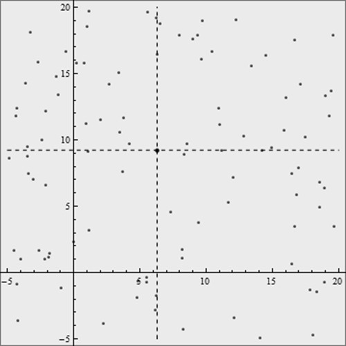
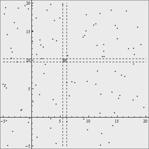
From the solutions above, we can see that Fermat point in norm-1 space may have infinity solutions. The visual representations with random 50 points in \mathbb​R2\mathbbsuperscript𝑅2\mathbb{R}^{2} space can be illustrated as follow.

Refer to caption
Refer to caption
Figure 1: Two possible cases of Fermat point(s) (marked in grey point or box) in β„’1superscriptβ„’1\mathcal{L}^{1} norm, in which left has one unique solution and right has infinity number of solutions.

3 Fermat Point in Euclidean Norm

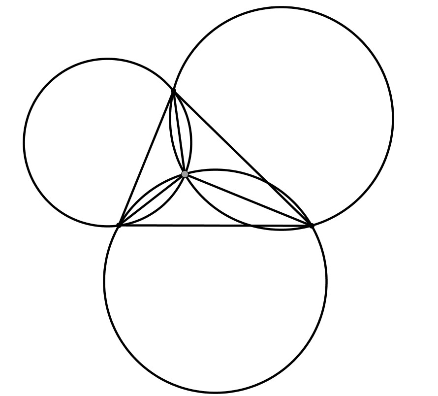
The unweighted 3-points problem in the Euclidean Norm is the original Fermat Problem. A solution to the one is to construct equilateral triangles on the sides with the vertices pointing outward. The intersected vertex from three circles is the Fermat point. The visualization is Figure 2, in which the black points are fixed points, and the grey point is the Fermat Point.
Refer to caption
Figure 2: Fermat point in a triangle

3.1 The Varignon Frame

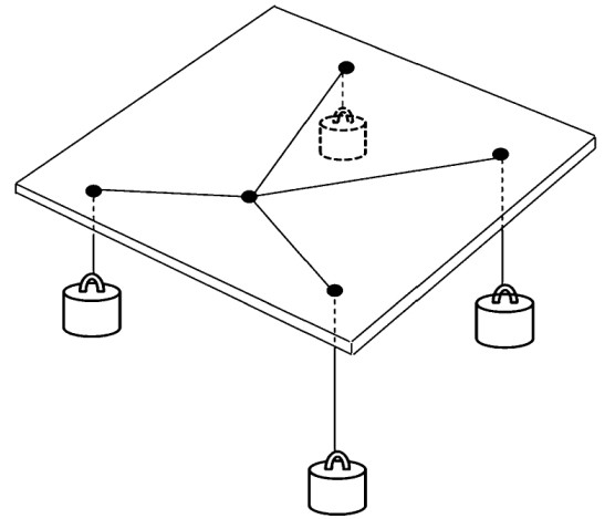
A good tool that allow us to inspire the general Fermat problem in Euclidean space is a mechanical analogue device The Varignon Frame named after the French mathematician Varignon. A board is drilled with mπ‘šm holes corresponding to the coordinates of the mπ‘šm fixed points. One string is fed through each hole and all strings are tied together in one knot. Below the board, weights are attached to the strings and proportional to the board. Given only gravity we concern and we ignore friction, the knot will settle at the optimal point. A graph of the Varignon frame is shown in Figure 3.[2]
Refer to caption
Figure 3: The Varignon Frame
Lemma 3.1.

The minimal potential energy point is the optimal point.

Proof.

Let the zero potential energy level is the ground, and height of this system is hβ„Žh, the length of each string is lisubscript𝑙𝑖l_{i}, and its weight is Gisubscript𝐺𝑖G_{i}, where i=1,2,β‹―,m𝑖12β‹―π‘ši=1,2,\cdots,m. We set up an initial point P𝑃P in this system, then we have

E​(P)=βˆ‘i=1mGi​[hβˆ’(liβˆ’P​MiΒ―)]=βˆ‘i=1mGi​(hβˆ’li)+βˆ‘i=1mGi​(P​MiΒ―)𝐸𝑃superscriptsubscript𝑖1π‘šsubscript𝐺𝑖delimited-[]β„Žsubscript𝑙𝑖¯𝑃subscript𝑀𝑖superscriptsubscript𝑖1π‘šsubscriptπΊπ‘–β„Žsubscript𝑙𝑖superscriptsubscript𝑖1π‘šsubscript𝐺𝑖¯𝑃subscript𝑀𝑖E(P)=\sum_{i=1}^{m}G_{i}[h-\left(l_{i}-\overline{PM_{i}}\,\right)]=\sum_{i=1}^{m}G_{i}(h-l_{i})+\sum_{i=1}^{m}G_{i}(\,\overline{PM_{i}}\,)

When P𝑃P is the minimal potential energy point, that is E​(P)𝐸𝑃E(P) is the minimum, βˆ‘i=1mGi​(P​MiΒ―)superscriptsubscript𝑖1π‘šsubscript𝐺𝑖¯𝑃subscript𝑀𝑖\sum_{i=1}^{m}G_{i}(\,\overline{PM_{i}}\,) reaches the minimum as βˆ‘i=1mGi​(hβˆ’li)superscriptsubscript𝑖1π‘šsubscriptπΊπ‘–β„Žsubscript𝑙𝑖\sum_{i=1}^{m}G_{i}(h-l_{i}) is the constant. ∎

3.2 The Weiszfeld’s Algorithm

The Weiszfeld’s iterative algorithm[3] was proposed to the Fermat problem in \mathbb​R2\mathbbsuperscript𝑅2\mathbb{R}^{2} space. The idea behind this algorithm, starting anywhere and trying to converge to 𝐅𝐅{\bf F}, is actually very simple. Let

𝐅=βˆ‘i=1m(βˆ‘j=1nki​|yjiβˆ’F|2)1/2.𝐅superscriptsubscript𝑖1π‘šsuperscriptsuperscriptsubscript𝑗1𝑛subscriptπ‘˜π‘–superscriptsuperscriptsubscript𝑦𝑗𝑖𝐹212{\bf F}=\sum_{i=1}^{m}\left(\sum_{j=1}^{n}k_{i}|y_{j}^{i}-F|^{2}\right)^{1/2}.

We assume π…βˆ‰π²i𝐅subscript𝐲𝑖{\bf F}\notin{\bf y}_{i}, then the negative of the gradient of f𝑓f at 𝐅𝐅{\bf F} equals,

R​(𝐅)=βˆ‘i=1mki​𝐲iβˆ’π…β€–π²iβˆ’π…β€–.𝑅𝐅superscriptsubscript𝑖1π‘šsubscriptπ‘˜π‘–subscript𝐲𝑖𝐅normsubscript𝐲𝑖𝐅R({\bf F})=\sum_{i=1}^{m}k_{i}\frac{{\bf y}_{i}-{\bf F}}{||{\bf y}_{i}-{\bf F}||}.

Therefore, let R​(𝐅)=0𝑅𝐅0R({\bf F})=0 which is equivalent to,

T​(𝐅)=βˆ‘i=1mki​𝐲iβ€–π…βˆ’π²iβ€–/βˆ‘i=1mkiβ€–π…βˆ’π²iβ€–,𝑇𝐅superscriptsubscript𝑖1π‘šsubscriptπ‘˜π‘–subscript𝐲𝑖norm𝐅subscript𝐲𝑖superscriptsubscript𝑖1π‘šsubscriptπ‘˜π‘–norm𝐅subscript𝐲𝑖T({\bf F})=\sum_{i=1}^{m}\frac{k_{i}{\bf y}_{i}}{\|{\bf F}-{\bf y}_{i}\|}/{\sum_{i=1}^{m}\frac{k_{i}}{\|{\bf F}-{\bf y}_{i}\|}},

as our iterative algorithm.

Rautenbach[7] proposed an extension Tβˆ—superscript𝑇T^{*} of T𝑇T to \mathbb​Rn\mathbbsuperscript𝑅𝑛\mathbb{R}^{n} space. Let P∈\mathbb​Rn,𝑃\mathbbsuperscript𝑅𝑛P\in\mathbb{R}^{n},

{If ​Tβˆ—β€‹(P)=P,Β if and only if ​P=𝐅(i)If ​Tβˆ—β€‹(P)β‰ P,Β then ​f​(Tβˆ—β€‹(P))<f​(P)(i​i).casesformulae-sequenceIfΒ superscript𝑇𝑃𝑃 if and only if 𝑃𝐅𝑖formulae-sequenceIfΒ superscript𝑇𝑃𝑃 then 𝑓superscript𝑇𝑃𝑓𝑃𝑖𝑖\begin{cases}\text{If }T^{*}(P)=P,\text{ if and only if }P={\bf F}&(i)\\ \text{If }T^{*}(P)\neq P,\text{ then }f(T^{*}(P))<f(P)&(ii)\end{cases}.

Kuhn[4] proved the part (i​i)𝑖𝑖(ii) and showed that, given an initial point X0∈\mathbb​Rnsubscript𝑋0\mathbbsuperscript𝑅𝑛X_{0}\in\mathbb{R}^{n}, the sequence of points {Xn}n∈Nsubscriptsubscript𝑋𝑛𝑛𝑁\left\{X_{n}\right\}_{n\in N} generated by the iterative process Xk+1=T​(Xk)subscriptπ‘‹π‘˜1𝑇subscriptπ‘‹π‘˜X_{k+1}=T\left(X_{k}\right) converges to the optimal solution of the Fermat problem if no point in the sequence is the vertex. In this last case, Kuhn claimed to have proved that this fact only occurs for a denumerable set of initial points. This result was modified by Chandrasekaran and Tamir [5], who gave two counterexamples and established the following conjecture: "If the convex hull of the set of vertices is of full dimension, then the set of initial points for which the sequence generated by the Weiszfeld’s algorithm yields in a vertex is denumerable."

Vardi and Zhang[6] improved the limit of Weiszfeld’s algorithm in case of π…βˆˆπ²i𝐅subscript𝐲𝑖{\bf F}\in{\bf y}_{i} appears in any iteration.

4 Fermat Point in Chebyshev Norm

The two dimensional Chebyshev distance has the similar property as the Manhattan distance. Hence, it can easily be viewed as the transformation of Manhattan distance, with the transformation matrix is

T=[220022]​[cos⁑π2βˆ’sin⁑π2sin⁑π2cos⁑π2].𝑇matrix220022matrixπœ‹2πœ‹2πœ‹2πœ‹2T=\begin{bmatrix}\frac{\sqrt{2}}{2}&0\\[3.00003pt] 0&\frac{\sqrt{2}}{2}\\[3.00003pt] \end{bmatrix}\begin{bmatrix}\cos{\frac{\pi}{2}}&-\sin{\frac{\pi}{2}}\\[3.00003pt] \sin{\frac{\pi}{2}}&\quad\!\cos{\frac{\pi}{2}}\\[3.00003pt] \end{bmatrix}.
Lemma 4.1.

β„’βˆžβ€‹(𝐲i,𝐅)=β„’1​(T​(𝐲i),T​(𝐅))superscriptβ„’superscript𝐲𝑖𝐅superscriptβ„’1𝑇superscript𝐲𝑖𝑇𝐅\mathcal{L}^{\infty}({\bf y}^{i},{\bf F})=\mathcal{L}^{1}(T({\bf y}^{i}),T({\bf F}))

Proof.
β„’1​(T​(y1i),T​(F))=22​|y1i​cos⁑π2+y2i​sin⁑π2βˆ’x1​sin⁑π2βˆ’x2​sin⁑π2|+22​|βˆ’y1i​cos⁑π2+y2i​sin⁑π2+x1​sin⁑π2βˆ’x2​sin⁑π2|=22max{12max{(y2iβˆ’x2+y2iβˆ’x2),(y1iβˆ’x1+y1iβˆ’x1),(βˆ’y1i+x1βˆ’y1i+x1),(βˆ’y2i+x2βˆ’y2i+x2)}}=max⁑{|y1iβˆ’x1|,|y2iβˆ’x2|}.superscriptβ„’1𝑇superscriptsubscript𝑦1𝑖𝑇𝐹22superscriptsubscript𝑦1π‘–πœ‹2superscriptsubscript𝑦2π‘–πœ‹2subscriptπ‘₯1πœ‹2subscriptπ‘₯2πœ‹222superscriptsubscript𝑦1π‘–πœ‹2superscriptsubscript𝑦2π‘–πœ‹2subscriptπ‘₯1πœ‹2subscriptπ‘₯2πœ‹22212superscriptsubscript𝑦2𝑖subscriptπ‘₯2superscriptsubscript𝑦2𝑖subscriptπ‘₯2superscriptsubscript𝑦1𝑖subscriptπ‘₯1superscriptsubscript𝑦1𝑖subscriptπ‘₯1superscriptsubscript𝑦1𝑖subscriptπ‘₯1superscriptsubscript𝑦1𝑖subscriptπ‘₯1superscriptsubscript𝑦2𝑖subscriptπ‘₯2superscriptsubscript𝑦2𝑖subscriptπ‘₯2superscriptsubscript𝑦1𝑖subscriptπ‘₯1subscriptsuperscript𝑦𝑖2subscriptπ‘₯2\begin{split}\mathcal{L}^{1}(T(y_{1}^{i}),T(F))&=\frac{\sqrt{2}}{2}\left|y_{1}^{i}\cos\frac{\pi}{2}+y_{2}^{i}\sin\frac{\pi}{2}-x_{1}\sin\frac{\pi}{2}-x_{2}\sin\frac{\pi}{2}\right|\\ &+\frac{\sqrt{2}}{2}\left|-y_{1}^{i}\cos\frac{\pi}{2}+y_{2}^{i}\sin\frac{\pi}{2}+x_{1}\sin\frac{\pi}{2}-x_{2}\sin\frac{\pi}{2}\right|\\ &=\frac{\sqrt{2}}{2}\max\bigg{\{}\frac{1}{\sqrt{2}}\max\big{\{}(y_{2}^{i}-x_{2}+y_{2}^{i}-x_{2}),(y_{1}^{i}-x_{1}+y_{1}^{i}-x_{1}),\\ &(-y_{1}^{i}+x_{1}-y_{1}^{i}+x_{1}),(-y_{2}^{i}+x_{2}-y_{2}^{i}+x_{2})\big{\}}\bigg{\}}\\ &=\max\left\{|y_{1}^{i}-x_{1}|,|y^{i}_{2}-x_{2}|\right\}.\end{split}

∎

However, the equivalence between β„’1​ andΒ β€‹β„’βˆžsuperscriptβ„’1Β andΒ superscriptβ„’\mathcal{L}^{1}\text{ and }\mathcal{L^{\infty}} cannot be generalized to the \mathbb​Rn\mathbbsuperscript𝑅𝑛\mathbb{R}^{n} due to the different properties on these two norms in higher dimensions.

5 Fermat Point in P𝑃P-Norm

The β„’psuperscriptℒ𝑝\mathcal{L}^{p} Space are the certain vector spaces of measurable functions. A vector space on which a norm is defined is called a normed vector space. It satisfies the following conditions,[8]

  • β€’

    β€–fβ€–>0norm𝑓0||f||>0 for fβ‰ 0𝑓0f\neq 0

  • β€’

    β€–0β€–=0norm00||0||=0

  • β€’

    β€–aβ‹…fβ€–=|a|β‹…β€–fβ€–normβ‹…π‘Žπ‘“β‹…π‘Žnorm𝑓||a\cdot f||=|a|\cdot||f|| for all a∈\mathbb​C1π‘Ž\mathbbsuperscript𝐢1a\in\mathbb{C}^{1}

  • β€’

    β€–f+g‖≀‖fβ€–+β€–gβ€–norm𝑓𝑔norm𝑓norm𝑔||f+g||\leq||f||+||g|| The Triangle Inequality.

For 0<pβ‰€βˆž0𝑝0<p\leq\infty we will denote the set of all ΞΌπœ‡\mu-measurable functions, f𝑓f, such that β€–fβ€–psuperscriptnorm𝑓𝑝||f||^{p} is integrable by β„’p​(X,β„±,ΞΌ)superscriptβ„’π‘π‘‹β„±πœ‡\mathcal{L}^{p}(X,\mathcal{F},\mu). We define a real-valued function, ||β‹…||p||\cdot||_{p}, on β„’psuperscriptℒ𝑝\mathcal{L}^{p} by ,

β€–fβ€–p=(βˆ«β€–f​(x)β€–p​𝑑μ​(x))1/p.subscriptnorm𝑓𝑝superscriptsuperscriptnorm𝑓π‘₯𝑝differential-dπœ‡π‘₯1𝑝||f||_{p}=\left(\int||f(x)||^{p}\,d\mu(x)\right)^{1/p}.

For 1≀p<∞1𝑝1\leq p<\infty this function is called the β„’psuperscriptℒ𝑝\mathcal{L}^{p}-norm. For 0<p<10𝑝10<p<1, β„’psuperscriptℒ𝑝\mathcal{L}^{p} is still a vector space, but ||β‹…||p||\cdot||_{p} is no longer a norm. Although ||β‹…||pp||\cdot||_{p}^{p} can be used to define an interesting metric on β„’psuperscriptℒ𝑝\mathcal{L}^{p}, we will not consider this case further.

Lemma 5.1.

If the points are not collinear, then f𝑓f is strictly convex.

Proof.

For X,Y,Q∈\mathbb​Rnπ‘‹π‘Œπ‘„\mathbbsuperscript𝑅𝑛X,Y,Q\in\mathbb{R}^{n}, and 0<t<10𝑑10<t<1, the Minkowski inequality shows,

β€–X+Yβ€–p≀‖Xβ€–p+β€–Yβ€–psubscriptnormπ‘‹π‘Œπ‘subscriptnorm𝑋𝑝subscriptnormπ‘Œπ‘||X+Y||_{p}\leq||X||_{p}+||Y||_{p}

implies,

||t(Xβˆ’\displaystyle||t(X- Q)+(1βˆ’t)(Yβˆ’Q)||p\displaystyle Q)+(1-t)(Y-Q)||^{p}
≀‖t​(Xβˆ’Q)β€–p+2​‖t​(Xβˆ’Q)β€–β‹…β€–(1βˆ’t)​(Yβˆ’Q)β€–+β€–(1βˆ’t)​(Yβˆ’Q)β€–pabsentsuperscriptnorm𝑑𝑋𝑄𝑝⋅2norm𝑑𝑋𝑄norm1π‘‘π‘Œπ‘„superscriptnorm1π‘‘π‘Œπ‘„π‘\displaystyle\leq||t(X-Q)||^{p}+2||t(X-Q)||\cdot||(1-t)(Y-Q)||+||(1-t)(Y-Q)||^{p}
=(t​‖Xβˆ’Qβ€–+(1βˆ’t)​‖Yβˆ’Qβ€–)pabsentsuperscript𝑑norm𝑋𝑄1𝑑normπ‘Œπ‘„π‘\displaystyle=(t||X-Q||+(1-t)||Y-Q||)^{p}

Hold if and only if X,Y,Qπ‘‹π‘Œπ‘„X,Y,Q are not collinear, therefore,

f​(t​X+(1βˆ’t)​Y)<t​f​(X)+(1βˆ’t)​f​(Y)𝑓𝑑𝑋1π‘‘π‘Œπ‘‘π‘“π‘‹1π‘‘π‘“π‘Œf(tX+(1-t)Y)<tf(X)+(1-t)f(Y)

∎

Since f​(x1,x2,β‹―,xn)𝑓subscriptπ‘₯1subscriptπ‘₯2β‹―subscriptπ‘₯𝑛f(x_{1},x_{2},\cdots,x_{n}) is convex, it proves that the Fermat point exists. Thus, by gradient descent

βˆ‡f=βˆ‚fβˆ‚xl(x1,x2,β‹―,xn=0,l=1,2,β‹―,n,\nabla f=\frac{\partial f}{\partial x_{l}}(x_{1},x_{2},\cdots,x_{n}=0,l=1,2,\cdots,n,

the function gets the minimum. It gives,

βˆ‚fβˆ‚xl(x1,x2,β‹―,xn)=βˆ‘i=1mβˆ‘j=1nki|yliβˆ’xl|pβˆ’1(|mjiβˆ’xj)|p)1/pβˆ’1yliβˆ’xlyliβˆ’x1=0,l=1,2,β‹―,n.\frac{\partial f}{\partial x_{l}}(x_{1},x_{2},\cdots,x_{n})=\sum_{i=1}^{m}\sum_{j=1}^{n}k_{i}|y_{l}^{i}-x_{l}|^{p-1}\left(\left|m_{j}^{i}-x_{j})\right|^{p}\right)^{1/p-1}\frac{\sqrt{y_{l}^{i}-x_{l}}}{y_{l}^{i}-x_{1}}=0,l=1,2,\cdots,n.

Therefore, we have our generalized iterative algorithm,

T​(xl)=βˆ‘i=1mβˆ‘j=1nkixli|yliβˆ’xl|pβˆ’1(|yliβˆ’xj)|2)p/2βˆ’1βˆ‘i=1mβˆ‘j=1nki|yliβˆ’xl|pβˆ’1(|yliβˆ’xj)|2)p/2βˆ’1,l=1,2,β‹―,n.T(x_{l})=\frac{\sum_{i=1}^{m}\sum_{j=1}^{n}k_{i}x_{l}^{i}|y_{l}^{i}-x_{l}|^{p-1}\left(\left|y_{l}^{i}-x_{j})\right|^{2}\right)^{p/2-1}}{\sum_{i=1}^{m}\sum_{j=1}^{n}k_{i}|y_{l}^{i}-x_{l}|^{p-1}\left(\left|y_{l}^{i}-x_{j})\right|^{2}\right)^{p/2-1}},\quad l=1,2,\cdots,n.

6 The Implement Test

We build the PASCAL-based programs for iterative algorithms we proposed in the above sections. The following tables below are the test results for random test points. In norm-1 or ∞\infty, the solution gives the exact result or range; in norm-2 and p𝑝p, the programs also add the precision as a condition. We set the first iteration as the gravity point of the system.

Input:   Number of Points    Dimension Weights
  4    6 2, 3, 1, 2
Test Points: (4, 11, 3, 4, 5, 6), (13, 13, 2, 1, 5, 7), (17, 6, 8, 6, 7, 8), (8, 6, 4, 6, 7, 9)
Output:   (8∼similar-to\sim13, 11, 3, 4, 5, 7)
Table 1: β„’psuperscriptℒ𝑝\mathcal{L}^{p} Algorithm
Input:  Number of Points   Precision    Dimension Weights
 6   0.001    2 1, 2, 4, 7, 6, 5
Test Points: (4.71, -1.84), (-3.15, -2.44), (0.17, 2.99),(6.35, 2.86), (5.55, 2.44), (3.22, -2.56)
Output: Start : (1.480, -0.140)
        ​ 1 : (1.713, 0.086)
        ​ 2 : (1.763, 0.124)
        ​ 3 : (1.776, 0.126)
        ​ 4 : (1.782, 0.122)
        ​ 5 : (1.787, 0.118)
        ​ 6 : (1.790, 0.115)
        ​ 7 : (1.793, 0.112)
        ​ 8 : (1.795, 0.110)
        ​ 9 : (1.798, 0.108)
        10: (1.799, 0.106)
        11: (1.801, 0.105)
        12: (1.802, 0.104)
Table 2: β„’2superscriptβ„’2\mathcal{L}^{2} Algorithm
Input: Number of Points Norm  Precision  Dimension Weights
5 2.4  0.00001  5 5, 9, 1, 8, 6
Test Points: (8, 5, 4, 8, 3), (3, 3, 7, 6, 3), (8, 7, 2, 6, 6), (4, 9, 3, 6, 2), (5, 6, 4, 5, 4)
Output: Start : (4.72414, 5.75862, 4.58621, 6.13793, 3.03448)
        ​ 1 : (4.95849, 5.91367, 4.57670, 5.74708, 3.46078)
        ​ 2 : (4.93330, 5.93940, 4.40332, 5.61458, 3.46066)
        ​ 3 : (4.94537, 5.99067, 4.38619, 5.56072, 3.53263)
        ​ 4 : (4.94590, 5.99950, 4.35138, 5.52565, 3.54720)
        ​ 5 : (4.94774, 6.01196, 4.34204, 5.50728, 3.56604)
        ​ 6 : (4.94833, 6.01319, 4.33222, 5.49539, 3.57347)
        ​ 7 : (4.94886, 6.01513, 4.32840, 5.48840, 3.57989)
        ​ 8 : (4.94909, 6.01562, 4.32523, 5.48396, 3.58315)
        ​ 9 : (4.94928, 6.01613, 4.32359, 5.48123, 3.58549)
        10: (4.94938, 6.01634, 4.32243, 5.47950, 3.58684)
        11: (4.94945, 6.01651, 4.32176, 5.47842, 3.58773)
        12: (4.94949, 6.01660, 4.32131, 5.47774, 3.58828)
        13: (4.94952, 6.01666, 4.32104, 5.47730, 3.58864)
        14: (4.94953, 6.01669, 4.32086, 5.47703, 3.58886)
        15: (4.94954, 6.01672, 4.32075, 5.47686, 3.58900)
        16: (4.94955, 6.01673, 4.32068, 5.47675, 3.58909)
        17: (4.94956, 6.01674, 4.32063, 5.47668, 3.58914)
        18: (4.94956, 6.01675, 4.32061, 5.47664, 3.58918)
        19: (4.94956, 6.01675, 4.32059, 5.47660, 3.58920)
        20: (4.94956, 6.01675, 4.32058, 5.47659, 3.58921)
Table 3: β„’psuperscriptℒ𝑝\mathcal{L}^{p} Algorithm

Acknowledgements

I would like to express my great gratitude to my adviser Donglei Gu and my friend Wilhelm Braum, for giving many insightful advices in this paper. Furthermore, I would like to thank my friend Liaoyuan Shen for the technical help in programming.

References

  • [1] Simpson, T. The Doctrine and application fluxions. Universidad de Salamanca, 1994.
  • [2] Eiselt, Horst A., and Carl-Louis Sandblom. Operations research: a model-based approach. Springer, 2012.
  • [3] Weiszfeld, Endre. "Sur le point pour lequel la somme des distances de n points donnΓ©s est minimum." Tohoku Math. J 43.355-386 (1937): 2.
  • [4] Kuhn, Harold W. "A note on Fermat’s problem." Mathematical programming 4.1 (1973): 98-107.
  • [5] Chandrasekaran, R., and A. Tamir. "Open questions concerning Weiszfeld’s algorithm for the Fermat-Weber location problem." Mathematical Programming 44.1-3 (1989): 293-295.
  • [6] Vardi, Yehuda, and Cun-Hui Zhang. "A modified Weiszfeld algorithm for the Fermat-Weber location problem." Mathematical Programming 90.3 (2001): 559-566.
  • [7] D. Rautenbach, M. Struzyna, C. Szegedy, J.Vygen, Weiszfeld’s Algorithm Revisited Once Again, Report No. 04946-OR, Research Institute for Discrete Mathematics, University of Bonn, 2004.
  • [8] Prugovecki, Eduard. Quantum mechanics in Hilbert space. Vol. 41. Access Online via Elsevier, 1982.