Statistical and Systematic Errors in Measurement of Weak-Lensing Minkowski Functionals: Application to Canada-France-Hawaii Lensing Survey

Abstract

The measurement of cosmic shear using weak gravitational lensing is a challenging task that involves a number of complicated procedures. We study in detail the systematic errors in the measurement of weak-lensing Minkowski Functionals (MFs). Specifically, we focus on systematics associated with galaxy shape measurements, photometric redshift errors, and shear calibration correction. We first generate mock weak-lensing catalogs that directly incorporate the actual observational characteristics of the Canada-France-Hawaii Lensing Survey (CFHTLenS). We then perform a Fisher analysis using the large set of mock catalogs for various cosmological models. We find that the statistical error associated with the observational effects degrades the cosmological parameter constraints by a factor of a few. The Subaru Hyper Suprime-Cam (HSC) survey with a sky coverage of $\sim 1400$ ${\rm deg}^{2}$ will constrain the dark energy equation of the state parameter with an error of $\Delta w_{0}\sim 0.25$ by the lensing MFs alone, but biases induced by the systematics can be comparable to the $1\sigma$ error. We conclude that the lensing MFs are powerful statistics beyond the two-point statistics, only if well-calibrated measurement of both the redshifts and the shapes of source galaxies is performed. Finally, we analyze the CFHTLenS data to explore the ability of the MFs to break degeneracies between a few cosmological parameters. Using a combined analysis of the MFs and the shear correlation function, we derive the matter density $\Omega_{\rm m0}=0.256\pm^{0.054}_{0.046}$.

1 INTRODUCTION

An array of recent observations such as cosmic microwave background (CMB) anisotropies (e.g., Komatsu et al., 2011; Hinshaw et al., 2013) and large-scale structure (e.g., Tegmark et al., 2006; Reid et al., 2010) established the standard $\Lambda$CDM model. The energy content of the present-day universe is dominated by dark energy and dark matter, and the primordial density fluctuations, which seeded all rich structure we observe today, were generated through an inflationary epoch in the very early universe. A few important questions still remain such as the nature of dark energy, the physical properties of dark matter, and the exact mechanism that generated the primordial density fluctuations.

Gravitational lensing is a powerful method for studying matter distribution in the universe, from which one can extract information on the basic cosmological parameters. The two-point correlation of galaxy ellipticities and the cross-correlation between galaxy positions and the shear caused by the underlying matter are popular statistics for constraining the cosmological model. These local statistics have been applied to real observational data and have provided independent and comparable cosmological constraints to those obtained using other measurements such as galaxy clustering (e.g., Kilbinger et al., 2013; Mandelbaum et al., 2013). Future weak-lensing surveys are aimed at measuring cosmic shear over a wide area of more than 1000 ${\rm deg}^{2}$. Such observational programs include Subaru Hyper Suprime-Cam (HSC), the Dark Energy Survey (DES), and the Large Synoptic Survey Telescope (LSST). The large set of cosmic shear data will enable us to improve the constraints on cosmological parameters which provides important clues to the mysterious dark components.

Several groups have explored statistics that make the best use of cosmic shear for cosmological parameter constraints. Minkowski Functionals (MFs) are among the most useful statistics to extract non-Gaussian information from a two-dimensional or three-dimensional field. Matsubara & Jain (2001) and Sato et al. (2001) study $\Omega_{\rm m0}$ dependence of weak-lensing MFs. More recently, Kratochvil et al. (2012) show that the lensing MFs contain significant cosmological information, beyond the power spectrum, whereas Shirasaki et al. (2012) show that weak-lensing MFs can be used to constrain the statistical properties of the primordial density fluctuations.

The true applicability of morphological statistics on observational cosmic-shear data needs to be further explored in detail. Previous studies on weak-lensing MFs often consider idealized conditions, assuming identical source redshift, homogeneous angular distribution of sources and/or perfectly calibrated shape measurement. Many observational effects in real weak-lensing measurement exist, however, that can be sources of systematic errors, for example, an imperfect shape measurement due to seeing and optical distortion, selection effects of source galaxies, uncertain redshift distribution of the source galaxies due to photometric redshift error (e.g., Bolzonella et al., 2000), noise-rectification biases (e.g., Kaiser, 2000; Erben et al., 2001; Hirata & Seljak, 2003), and complicated survey geometry due to mask regions (Shirasaki et al., 2013). Some of these effects on cosmic-shear power spectrum analysis have been already studied (e.g., Huterer et al., 2006; Hikage et al., 2011). It is timely and important to conduct a comprehensive study of observational effects on lensing MFs, in order to fully exploit the data from upcoming wide-cosmology surveys.

Earlier in Shirasaki et al. (2013), we studied the effect of mask regions on the measurement of weak-lensing MFs. Geometrical constraints due to masks can be a major source of systematics because MFs are intrinsically morphological quantities. We showed that sky-masking induces large non-Gaussianities, which could compromise measurement of the true non-Gaussianity associated with gravitational growth. We thus argue that it is important to include directly realistic observational effects in order to apply the lensing MFs to data from future cosmology surveys.

In the present paper, we further explore several observational effects using the real data set from the Canada-France-Hawaii Lensing Survey (CFHTLenS). We use a large set of simulations to study possible systematics in detail one by one. We finally present a forecast for future surveys such as Subaru HSC and LSST. The rest of the present paper is organized as follows. In Section 2, we summarize the basics of lensing statistics of interest and how to estimate MFs from the observed shear field. In Section 3, we describe the data used in this paper and the details of weak-lensing mock catalogs for morphological analysis are found in Section 4. In Section 5, we show the results of the impact of observational effects on lensing MFs. We perform a Fisher analysis to present a realistic forecast by using a large set of weak-lensing mock catalogs. In Section 6, we apply our statistical method to real data to quantify the power of lensing MFs as a cosmology probe. Concluding remarks and discussions are given in Section 7.

2 WEAK-LENSING STATISTICS

We summarize the basics of gravitational lensing by large-scale structure. Let us denote the observed position of a source object as $\theta$ and the true position as $\beta$. Then the image distortion of a source object is characterized by the following two-dimensional (2D) matrix:

$$A_{ij}=\frac{\partial\beta^{i}}{\partial\theta^{j}}\equiv\left(\begin{array}[]{cc}1-\kappa-\gamma_{1}&-\gamma_{2}\\ -\gamma_{2}&1-\kappa+\gamma_{1}\\ \end{array}\right),$$ (3)

where $\kappa$ is convergence and $\gamma=\gamma_{1}+i\gamma_{2}$ is shear. In a weak-lensing regime (i.e., $\kappa,\gamma\ll 1$), each component of $A_{ij}$ can be related to the second derivative of the lensing potential $\Phi$ (Bartelmann & Schneider, 2001; Munshi et al., 2008). The lensing potential is calculated from the weighted integral of gravitational potential along a line of sight, and the Poisson equation relates the gravitational potential field to the matter over-density field $\delta$. Weak-lensing convergence field is then given by

$$\kappa(\mbox{\boldmath$\theta$},\chi) = \int_{0}^{\chi_{H}}{\rm d}\chi\,W(\chi)\delta(r(\chi)\mbox{\boldmath$\theta$},\chi),$$ (4)

$$W(\chi) = \frac{3}{2}\left(\frac{H_{0}}{c}\right)^{2}\Omega_{\rm m0}\frac{r(\chi)}{a(\chi)}\int_{\chi}^{\chi_{H}}{\rm d}\chi^{\prime}p(\chi^{\prime})\frac{r(\chi^{\prime}-\chi)}{r(\chi^{\prime})},$$ (5)

where $\chi$ is the comoving coordinate, $r(\chi)$ is the angular diameter distance, and $p(\chi)$ represents the redshift distribution of sources.

2.1 Two Point Statistics

By using the Limber approximation (Limber, 1954; Kaiser, 1992) and Equation (4), one can calculate the convergence power spectrum as

$$P_{\kappa}(\ell) = \int_{0}^{\chi_{s}}{\rm d}\chi\frac{W(\chi)^{2}}{r(\chi)^{2}}P_{\delta}\left(k=\frac{\ell}{r(\chi)},z(\chi)\right),$$ (6)

where $P_{\delta}(k)$ is the three-dimensional matter power spectrum. The most direct measurement of weak-lensing two-point statistics is the two-point shear correlation function (2PCF) $\xi_{\pm}$. Theoretically, the 2PCFs are obtained by the Hankel transforms of a convergence power spectrum $P_{\kappa}$ as

$$\xi_{\pm}(\theta)=\frac{1}{2\pi}\int_{0}^{\infty}{\rm d}\ell\,\ell\,P_{\kappa}(\ell)\,J_{0,4}(\ell\theta),$$ (7)

where $J_{0}$ and $J_{4}$ are the first-kind Bessel functions of the order 0 and 4.

Schneider et al. (2002) show that the 2PCFs are estimated in an unbiased way by averaging over pairs of galaxies. In practice, the estimator $\hat{\xi}_{\pm}$ is calculated by

$$\hat{\xi}_{\pm}(\theta)=\frac{\sum_{ij}w_{i}w_{j}\left(\epsilon_{t}(\mbox{\boldmath$\theta$}_{i})\epsilon_{t}(\mbox{\boldmath$\theta$}_{j})+\epsilon_{\times}(\mbox{\boldmath$\theta$}_{i})\epsilon_{\times}(\mbox{\boldmath$\theta$}_{j})\right)}{\sum_{ij}w_{i}w_{j}},$$ (8)

where $w_{i}$ is weight related to shape measurement and $\epsilon_{t,\times}(\mbox{\boldmath$\theta$}_{i})$ is the tangential and cross component of $i$th source galaxy’s ellipticity. The summation is taken over all galaxy pairs $(i,j)$ with angular separation $|\mbox{\boldmath$\theta$}_{i}-\mbox{\boldmath$\theta$}_{j}|\in[\theta-\Delta\theta,\theta+\Delta\theta]$.

2.2 Minkowski Functionals

MFs are morphological statistics for some smoothed random fields characterized by a certain threshold. In general, for a given $D$-dimensional smoothed field $\mathbb{S}^{D}$, one can calculate $D+1$ MFs $V_{i}$. One can thus define 2+1 MFs on $\mathbb{S}^{2}$: $V_{0},V_{1}$ and $V_{2}$. The MFs are defined, for a threshold of $\nu$, as

$$V_{0}(\nu) \equiv \frac{1}{4\pi}\int_{Q_{\nu}}\,{\rm d}S,$$ (9)

$$V_{1}(\nu) \equiv \frac{1}{4\pi}\int_{\partial Q_{\nu}}\,\frac{1}{4}{\rm d}\ell,$$ (10)

$$V_{2}(\nu) \equiv \frac{1}{4\pi}\int_{\partial Q_{\nu}}\,\frac{1}{2\pi}K{\rm d}\ell,$$ (11)

where $Q_{\nu}$ and $\partial Q_{\nu}$ represent the excursion set and its boundaries for a smoothed field $u(\mbox{\boldmath$\theta$})$. They are given by

$$Q_{\nu}=\{\mbox{\boldmath$\theta$}\,|\,u(\mbox{\boldmath$\theta$})>\nu\},$$ (12)

$$\partial Q_{\nu}=\{\mbox{\boldmath$\theta$}\,|\,u(\mbox{\boldmath$\theta$})=\nu\}.$$ (13)

For a given threshold, $V_{0}$, $V_{1}$ and $V_{2}$ describe the fraction of sky area, the total boundary length of contours, and the integral of the geodesic curvature $K$ along the contours, respectively.

2.3 Measuring Lensing MFs from Cosmic Shear Data

We summarize how to estimate lensing MFs from observed cosmic shear. Let us first define the weak-lensing mass map, i.e., the smoothed lensing convergence field:

$${\cal K}(\mbox{\boldmath$\theta$})=\int{\rm d}^{2}\phi\ \kappa(\mbox{\boldmath$\theta$}-\mbox{\boldmath$\phi$})U(\mbox{\boldmath$\phi$}),$$ (14)

where $U$ is the filter function to be specified below. We can calculate the same quantity by smoothing the shear field $\gamma$ as

$${\cal K}(\mbox{\boldmath$\theta$})=\int{\rm d}^{2}\phi\ \gamma_{t}(\mbox{\boldmath$\phi$}:\mbox{\boldmath$\theta$})Q_{t}(\mbox{\boldmath$\phi$}),$$ (15)

where $\gamma_{t}$ is the tangential component of the shear at position $\phi$ relative to the point $\theta$. The filter function for the shear field $Q_{t}$ is related to $U$ by

$$Q_{t}(\theta)=\int_{0}^{\theta}{\rm d}\theta^{\prime}\ \theta^{\prime}U(\theta^{\prime})-U(\theta).$$ (16)

We consider $Q_{t}$ to be defined with a finite extent. In this case, one finds

$$U(\theta)=2\int_{\theta}^{\theta_{o}}{\rm d}\theta^{\prime}\ \frac{Q_{t}(\theta^{\prime})}{\theta^{\prime}}-Q_{t}(\theta),$$ (17)

where $\theta_{o}$ is the outer boundary of the filter function.

In the following, we consider the truncated Gaussian filter (for $U$) as

$$U(\theta) = \frac{1}{\pi\theta_{G}^{2}}\exp\left(-\frac{\theta^{2}}{\theta_{G}^{2}}\right)-\frac{1}{\pi\theta_{o}^{2}}\left(1-\exp\left(-\frac{\theta_{o}^{2}}{\theta_{G}^{2}}\right)\right),$$ (18)

$$Q_{t}(\theta) = \frac{1}{\pi\theta^{2}}\left[1-\left(1+\frac{\theta^{2}}{\theta_{G}^{2}}\right)\exp\left(-\frac{\theta^{2}}{\theta_{G}^{2}}\right)\right],$$ (19)

for $\theta\leq\theta_{o}$ and $U=Q_{t}=0$ elsewhere. Throughout the present paper, we adopt $\theta_{G}=1$ arcmin and $\theta_{o}=15$ arcmin. Note that this choice of $\theta_{G}$ is considered to be an optimal smoothing scale for the detection of massive galaxy clusters using weak-lensing for $z_{\rm source}$ = 1.0 (Hamana et al., 2004).

It is important to use appropriately the weight associated with shape measurement when making smoothed convergence maps. In practice, we estimate ${\cal K}$ by generalizing Equation (15):

$${\cal K}(\mbox{\boldmath$\theta$}_{i})=\frac{\sum_{j}Q_{t}(\mbox{\boldmath$\phi$}_{j})w_{j}\epsilon_{t}(\mbox{\boldmath$\phi$}_{j}:\mbox{\boldmath$\theta$}_{i})}{\sum_{j}Q_{t}(\mbox{\boldmath$\phi$}_{j})w_{j}},$$ (20)

where the summation in Equation (20) is taken over all the source galaxies that are located within $\theta_{o}$ from $i$th pixel. The weak-lensing convergence field ${\cal K}$ is then computed from the galaxy ellipticity data on regular grids with a grid spacing of 0.15 arcmin. In making the convergence map, we discard the pixels when the denominator in Equation (20) is equal to zero. The boundaries are defined by masking a pixel if the number of sources within $\theta_{o}$ from the pixel is less than $5\sqrt{15\pi\theta_{o}^{2}}$. This critical value effectively sets the signal-to-noise ratio of the number of sources inside a circle with radius of $\theta_{o}$ to be less than 5, on the assumption that the distribution of sources is approximated by a Poisson distribution. We repeat the above procedure for all the pixels. Note that the details of the procedure do not affect the final results significantly as long as we impose the same conditions to on all of the pixels, because our analysis is based on the comparison of two maps that have the same configuration of source positions.

We follow Lim & Simon (2012) to calculate the MFs from pixelated ${\cal K}$ maps. We convert a weak-lensing field ${\cal K}$ to $x=({\cal K}-\langle{\cal K}\rangle)/\sigma_{0}$ where $\sigma_{0}$ is the standard deviation of ${\cal K}$. We set $\Delta x=0.2$ from $x=-5$ to $x=5$ for binning the threshold value.

3 DATA

We use the data from the Canada-France-Hawaii Telescope Lensing Survey (CFHTLenS; Heymans et al., 2012). CFHTLenS is a 154 ${\rm deg}^{2}$ multi-color optical survey in the five optical bands $u^{*},g^{\prime},r^{\prime},i^{\prime},\ {\rm and}\ z^{\prime}$. CFHTLenS is optimized for weak-lensing analysis with a full multi-color depth of $i^{\prime}_{AB}=24.7$ with optimal sub-arcsecond seeing conditions. The survey consists of four separated regions called W1, W2, W3 and W4, with an area of $\sim$ 72, 30, 50 and 25 ${\rm deg}^{2}$, respectively.

The CFHTLenS survey analysis mainly consists of the following processes: weak-lensing data processing with THELI (Erben et al., 2013), shear measurement with the $lens$fit (Miller et al., 2013), and photometric redshift measurement (Hildebrandt et al., 2012). A detailed systematic error study of the shear measurements in combination with the photometric redshifts is presented in Heymans et al. (2012). The additional error analyses of the photometric redshift measurements are presented in Benjamin et al. (2013).

The ellipticities of the source galaxies in the data have been calculated using the $lens$fit algorithm. The $lens$fit performs a Bayesian model fitting to the imaging data by varying a galaxy’s ellipticity and size, and by marginalizing over the centroid position. It takes into account a forward convolution process expressed by convolving the galaxy model with the point-spread function (PSF) to estimate the posterior probability of the model given the data. For each galaxy, the ellipticity $\epsilon$ is estimated as the mean likelihood of the model posterior probability after marginalizing over galaxy size, centroid position, and bulge fraction. An inverse variance weight $w$ is given by the variance of the ellipticity likelihood surface and the variance of the ellipticity distribution of the galaxy population (see Miller et al. (2013) for further details).

The photometric redshifts $z_{p}$ are estimated by the BPZ code (Benítez, 2000, Bayesian Photometric Redshift Estimation). Benjamin et al. (2013) shows that the true redshift distribution is well described by the sum of the probability distribution functions (PDFs) estimated from BPZ. The galaxy-galaxy-lensing redshift scaling analysis of Heymans et al. (2012) confirms that contamination is unimportant for galaxies selected at $0.2<z_{p}<1.3$. In this redshift range, the weighted median redshift is $\sim 0.7$ and the effective weighted number density $n_{\rm eff}$ is 11 per ${\rm arcmin}^{2}$. We have used the source galaxies with $0.2<z_{p}<1.3$ to make the smoothed lensing mass map analyzed in 2.3.

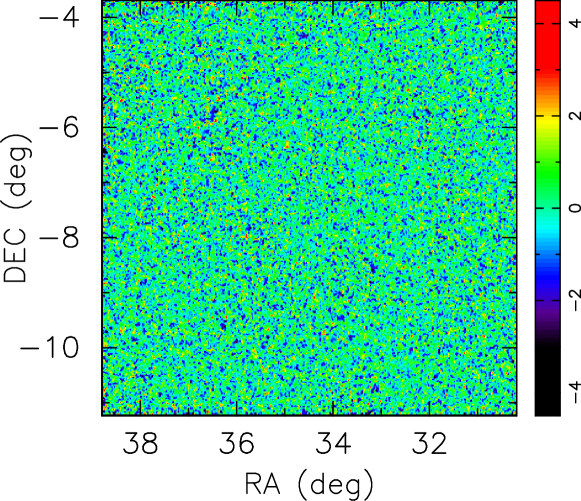
The effective survey area is an important quantity for our study. Heymans et al. (2012) perform systematic tests in order to mark and remove data with significant residual systematics. The fraction of data flagged by their procedure amounts to 25 % of the total CFHTLenS; this is indeed significant. Our previous work (Shirasaki et al., 2013) shows that the cosmological information content in the lensing MFs is largely determined by the effective survey area. More importantly, however, complicated geometries of the masked regions induce non-Gaussianities that contaminate the lensing MFs. We have decided to use all the available data of CFHTLenS to make a wide and continuous map. We expect the systematics associated with the PSF to be relatively small compared to the masking effect on morphological statistics (see, e.g., Heymans et al. (2012); Van Waerbeke et al. (2013)). To calculate the 2PCF, we use the clean sample of Heymans et al. (2012). We show the obtained mass map in the CFHTLenS W1 field in Figure 1.

Figure 1: Reconstructed convergence field ${\cal K}$ in the CFHTLenS W1 field. The ${\cal K}$ map is calculated from the ellipticities of 2570270 source galaxies. The color-scale bar shows the normalized value $({\cal K}-\langle{\cal K}\rangle)/\sigma_{0}$.

4 SIMULATIONS

4.1 Ray-Tracing Simulation

We first run a number of cosmological $N$-body simulations to generate a three-dimensional matter density field. We use the parallel Tree-Particle Mesh code Gadget2 (Springel, 2005). The simulations are run with $512^{3}$ dark matter particles in a volume of $480$ or $960\ h^{-1}$Mpc on a side. We generate the initial conditions using a parallel code developed by Nishimichi et al. (2009) and Valageas & Nishimichi (2011), which employs the second-order Lagrangian perturbation theory (e.g., Crocce et al., 2006). The initial redshift is set to $z_{\rm init}=50$, where we compute the linear matter transfer function using CAMB (Lewis et al., 2000). Our fiducial cosmology adopts the following parameters: matter density $\Omega_{\rm m0}=0.279$, dark energy density $\Omega_{\Lambda 0}=0.721$, the amplitude of curvature fluctuations $A_{s}=2.41\times 10^{-9}$ at the pivot scale $k=0.002{\rm Mpc}^{-1}$, the parameter of the equation of state of dark energy $w_{0}=-1$, Hubble parameter $h=0.700$ and the scalar spectral index $n_{s}=0.972$. These parameters are consistent with the WMAP nine-year results (Hinshaw et al., 2013). To investigate the degeneracy of the cosmological parameters, we also run the same set of simulations but with slightly different $\Omega_{\rm m0}$, $w_{0}$ and $A_{s}$. We summarize the simulation parameters in Table 1.

For ray-tracing simulations of gravitational lensing, we generate light-cone outputs using multiple simulation boxes in the following manner. Our small- and large-volume simulations are placed to cover the past light-cone of a hypothetical observer with an angular extent $10^{\circ}\times 10^{\circ}$, from $z=0$ to $3$, similarly to the methods in White & Hu (2000), Hamana & Mellier (2001), and Sato et al. (2009). Details of the configuration are found in the last reference. The angular grid size of our maps is $10^{\circ}/4096\sim 0.15$ arcmin. We use outputs from independent realizations when generating the light-cone outputs. We also randomly shift the simulation boxes in order to avoid the same structure appearing multiple times along a line-of-sight. In total, we generate 40 independent shear maps from four $N$-body simulations for each cosmological model.

	$\Omega_{\rm m0}$	$w_{0}$	$A_{s}\times 10^{9}$	$\sigma_{8}$	# of $N$-body sims	# of maps
Fiducial	0.279	-1.0	2.41	0.823	4	40
High $\Omega_{\rm m0}$	0.304	-1.0	2.41	0.878	4	40
Low $\Omega_{\rm m0}$	0.254	-1.0	2.41	0.763	4	40
High $w_{0}$	0.279	-0.8	2.41	0.768	4	40
Low $w_{0}$	0.279	-1.2	2.41	0.862	4	40
High $A_{s}$	0.279	-1.0	2.51	0.840	4	40
Low $A_{s}$	0.279	-1.0	2.31	0.806	4	40

Table 1: Parameters for our $N$-body simulations. We also show the resulting $\sigma_{8}$. For each parameter set, we run 4 $N$-body realizations and generate 40 weak-lensing shear maps.

4.2 Mock Weak-Lensing Catalogs

Our purpose is to study observational effects on weak-lensing morphological statistics. To this end, we generate realistic mock weak-lensing catalogs by combining ray-tracing simulations and the CFHTLenS data (Van Waerbeke et al., 2013). The main advantage of our mock catalogs is that the observed positions on the sky of the source galaxies are directly used. Because of this, we can keep all the characteristics of the survey geometry the same as in CFHTLenS.

We locate the source galaxies in the pixel unit of our lensing map and then calculate the reduced shear signal $g=\gamma/(1-\kappa)$ at the galaxy positions. Ray-tracing is done up to the redshift of the galaxy as described in Section 4.1. In this step, a galaxy’s redshift is set to be at the peak of the posterior PDF obtained from BPZ. This could cause systematic effects on morphological statistics originating from the inaccuracy of the photometric redshift estimation. We discuss the impact of the redshift distribution of sources on lensing morphological statistics later in Section 5.

We next consider the intrinsic ellipticity that is known to be a major error source in cosmic shear measurement. For each galaxy, we randomize the orientation of the observed ellipticity, while keeping its amplitude. The randomized ellipticity is then assigned as the intrinsic ellipticity $\epsilon_{\rm int}$ at each galaxy’s position. Seitz & Schneider (1997) show that the observed source ellipticity sheared by weak-lensing effect can be expressed as a function of $\epsilon_{\rm int}$ and the reduced shear signal $g$. The final “observed” ellipticity is

$${\mbox{\boldmath$\epsilon$}}_{\rm mock}=\frac{{\mbox{\boldmath$\epsilon$}}_{\rm int}+{\mbox{\boldmath$g$}}}{1+{\mbox{\boldmath$g$}}^{*}{\mbox{\boldmath$\epsilon$}}_{\rm int}},$$ (21)

where ${\mbox{\boldmath$\epsilon$}}_{\rm mock}$ is represented as a complex ellipticity.

Finally, we incorporate calibration correction in the shear measurement. We assign the weight associated with the shape measurement of $lens$fit and the shear calibration correction following Heymans et al. (2012). The two factors determine the potential additive shear bias $c$ and multiplicative bias $m$. We then apply the shear calibration correction to ${\mbox{\boldmath$\epsilon$}}_{\rm mock}$ by using bias factors $m$ and $c$ as

$${\mbox{\boldmath$\epsilon$}}_{\rm mock}\rightarrow(1+m){\mbox{\boldmath$\epsilon$}}_{\rm mock}+{\mbox{\boldmath$c$}}.$$ (22)

In this step, we assume that there is no correlation between $\epsilon$ and $m,\mbox{\boldmath$c$}$. We have explicitly calculated the correlation between $\epsilon$ and $m,\mbox{\boldmath$c$}$ at the source galaxy positions using the CFHTLenS data set, and found that there is indeed no significant correlation between the quantities.

Through the above procedures, we have successfully included the following observational effects in our analysis: (1) non-linear relation between the observed ellipticities and cosmic shear, (2) non-Gaussian distribution of the intrinsic ellipticities, (3) the masked survey area of CFHTLenS and the inhomogeneous angular distribution of the source galaxies, (4) imperfect shape measurements and (5) the redshift distribution of the source galaxies. We note that all or many of these effects are often ignored in previous works on lensing morphological statistics.

5 REALISTIC FORECAST

5.1 Fisher Analysis

We perform a Fisher analysis to produce a forecast for parameter constraints on $\Omega_{\rm m0}$, $A_{s}$, and $w_{0}$ with future weak-lensing surveys.

For a multivariate Gaussian likelihood, the Fisher matrix $F_{ij}$ can be written as

$$F_{ij}=\frac{1}{2}{\rm Tr}\left[A_{i}A_{j}+C^{-1}M_{ij}\right],$$ (23)

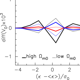
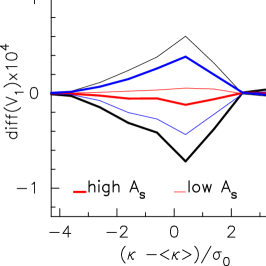
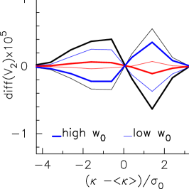
where $A_{i}=C^{-1}\partial C/\partial p_{i}$, $M_{ij}=2\left(\partial\mu/\partial p_{i}\right)\left(\partial\mu/\partial p_{j}\right)$, $C$ is the data covariance matrix, $\mu$ represents the assumed model, and $\mbox{\boldmath$p$}=(\Omega_{\rm m0},A_{s},w_{0})$ are the main parameters. In the present study, we consider only the second term in Equation (23). Because $C$ is expected to scale proportionally inverse to the survey area, the second term will be dominant for a large area survey (see, e.g., Eifler et al. (2009)). We calculate the model template by averaging the MFs over 40 convergence maps with appropriate noises for each CFHTLenS field. Figure 2 shows the cosmological dependence of our model MFs thus calculated. We see clearly the behavior of the MFs as a function of $p$.

We calculate the model 2PCFs using the fitting formula of non-linear matter power spectrum of Takahashi et al. (2012), on the assumption that the source redshift distribution is well approximated by the sum of the posterior PDF with $0.2<z_{p}<1.3$ given in Kilbinger et al. (2013).

Figure 2: Variation of the lensing MFs for different cosmological parameters. We plot the differences of $V_{0},V_{1}$, and $V_{2}$. with respect to those of our fiducial cosmology. In all of the panels, the thick (thin) black line corresponds to the case of cosmological model with higher (lower) $\Omega_{\rm m0}$. The thick (thin) red one shows the result of the cosmological model with higher (lower) $A_{s}$, and the thick (thin) blue one is for the model with higher (lower) $w_{0}$. For reference, the typical statistical errors of $V_{0}$,$V_{1}$, and $V_{2}$ at $({\cal K}-\langle{\cal K}\rangle)/\sigma_{0}=0$ are $\sim 10^{-3}$, $10^{-4}$, and $10^{-5}$, respectively, for CFHTLenS.

To calculate the matrix $M_{ij}$, we approximate the first derivatives of the 2PCF and MFs with respect to cosmological parameter $p_{i}$ as

$$\frac{\partial\mu}{\partial p_{i}}=\frac{\mu(p^{(0)}_{i}+\Delta p_{i})-\mu(p^{(0)}_{i}-\Delta p_{i})}{2\Delta p_{i}},$$ (24)

where $\mbox{\boldmath$p$}^{(0)}=(0.279,2.41\times 10^{-9},-1.0)$ gives our fiducial model parameters and we set $\Delta\mbox{\boldmath$p$}=(0.025,0.1\times 10^{-9},0.2)$.

We construct the data vector $D$ from a set of binned MFs and 2PCFs,

$${D_{i}}=\{V_{0}(x_{1}),...,V_{0}(x_{10}),V_{1}(x_{1}),...,V_{1}(x_{10}),V_{2}(x_{1}),...,V_{2}(x_{10}),$$

$$\xi_{+}(\theta_{1}),...,\xi_{+}(\theta_{10}),\xi_{-}(\theta_{1}),...,\xi_{-}(\theta_{10})\},$$ (25)

where $x_{i}=({\cal K}_{i}-\langle{\cal K}\rangle)/\sigma_{0}$ is the binned normalized lensing field. For the Fisher analysis, we use 10 bins in the range of $x_{i}=[-3,3]$ . In this range of $x$, Equation (24) gives smooth estimates for $M_{ij}$. For the 2PCFs, we use 10 bins logarithmically spaced in the range of $\theta_{i}=[0.9,300]$ arcmin. A data vector has 50 elements, $3\times 10$ MFs and $2\times 10$ 2PCFs, in total.

We therefore need a $50\times 50$ data covariance matrix for the Fisher analysis. To this end, we first use 1000 shear maps made by Sato et al. (2009). The maps have almost the same design as our simulations, but are generated for slightly different cosmological parameters (consistent with WMAP three-years results (Spergel et al., 2007)). The actual parameter differences are small, and also the dependence of the covariance matrix on cosmological parameters is expected to be weak. Each map covers a $5^{\circ}\times 5^{\circ}$ sky and the source redshift is set to be $z_{\rm source}=1$. We model the intrinsic ellipticities by adding random ellipticities drawn from a 2D Gaussian to the simulated shear data. We set the rms of the intrinsic ellipticities to be 0.38 and the number of source galaxies is set to be 10 ${\rm arcmin}^{-2}$. These are reasonable choices for our study here. In making the smoothed lensing map from the simulation outputs, we set the weight related to shape measurement to be unity. From the 1000 shear maps with appropriate noises, we can estimate the variances of the 2PCFs and MFs. We also estimate the statistical errors by randomly rotating the observed orientation of the ellipticities. Using these randomized catalogs, the data covariance matrices in each CFHTLenS field can be estimated by the sum of sampling variance and the statistical error as

$$C_{\rm each}=C_{\rm cosmic}\left(\frac{A_{\rm each}\ {\rm deg}^{2}}{25\ {\rm deg}^{2}}\right)^{-1}+C_{\rm stat},$$ (26)

where $C_{\rm cosmic}$ is sampling variance, $C_{\rm stat}$ represents the statistical error in each CFHTLenS field, and $A_{\rm each}$ corresponds to the effective survey area. In the following, we assume that the four CFHTLenS fields are independent of each other statistically. The total inverse covariance matrix for the whole CFHTLenS data is the sum of $C_{\rm each}^{-1}$ over the W1, W2, W3 and W4 fields. We forecast for future lensing surveys by simply scaling the data covariances by the survey area, assuming that the statistical error is identical to that in CFHTLenS. When calculating the inverse covariance, we include a debiasing correction, the so-called Anderson-Hartlap factor $\alpha=(n_{\rm real}-n_{\rm bin}-2)/(n_{\rm real}-1)$ with $n_{\rm rea}=1000$ being the number of realization of simulation sets and $n_{\rm bin}=50$ being the number of total bins in our data vector (Hartlap et al., 2007).

We expect that Equation (26) provides a good approximation to the full covariance, but the accuracy needs to be addressed here. In the case of shear correlation functions, the covariance matrix consists of three components: a sampling variance, the statistical noise, and a third term coupling the two (Schneider et al., 2002). Because the MFs do not have the additivity of, e.g., $V_{i}(\nu_{1}+\nu_{2})=V_{i}(\nu_{1})+V_{i}(\nu_{2})$, it is not clear if the MF covariance can be expressed similarly as the sum of the three contributions. We thus resort to estimating the MF covariance in a direct manner by using the large set of mock catalogs generated by the procedure shown in Section 4.2. Note that, in the procedure, we perform two randomization processes for a fixed cosmological model. One is to generate multiple realizations of the large scale structure (by $N$-body simulations) and the other is to randomize intrinsic ellipticities of the source galaxies. We perform each process separately, technically by fixing a random seed of the other process, to evaluate each term in Equation (26). In principle, one can perform both of the processes simultaneously and derive the full covariance. However, this would require a huge number of mock catalogs. In Appendix B, we have done a simple but explicit check to validate that Equation (26) indeed provides a reasonably good approximation. The details of our test and the result are shown there.

5.2 Forecast for Upcoming Survey

We present a forecast for upcoming surveys such HSC and LSST. We first derive constraints on the cosmological parameters for a 154 ${\rm deg}^{2}$ area survey, for which we have the full covariance matrix obtained in the previous sections. We then consider two wide surveys with an area coverage of 1400 ${\rm deg}^{2}$ (HSC) and 20000 ${\rm deg}^{2}$ (LSST). We simply scale the covariance matrix by a factor of $154/1400$ or $154/20000$ for them.

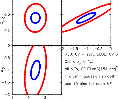
Let us begin with quantifying the statistical error associated with the real data. We have performed a Fisher analysis including the sampling variance and the statistical error. When we include the statistical error, the cosmological constraints are degraded by a factor of $\sim 2$ for the CHFTLens survey. In Figure 3, the red error circle corresponds to the 1$\sigma$ cosmological constraints including the sampling variance and the statistical error, while the blue one is obtained from the Fisher analysis without the statistical error.

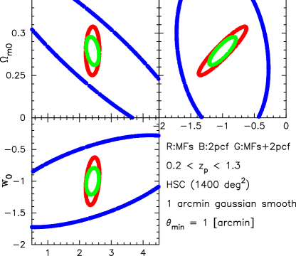
We are now able to present a forecast for future lensing surveys covering larger sky areas on the assumption that the data covariance is the same as that of CFHTLenS. Figure 4 shows the derived parameter constraints. The blue error circles show the 1$\sigma$ constraints from the shear 2PCFs whereas the red circles are obtained from the lensing MFs. It is promising that, with Subaru HSC, we can constrain the dark energy equation of state $w_{0}$ with an error of $\Delta w_{0}\sim 0.25$ by the lensing MFs alone. Table 2 summarizes the expected constraints by future surveys. Combining the 2PCFs and the MFs can improve the constraints by a factor of $\sim 2$ by breaking the degeneracy between the three parameters. It should be noted that this conclusion might seem slightly different from that of Kratochvil et al. (2012), who argue that adding the power spectrum does not effectively improve the constraints when all three MFs are already used. Our result suggests that combining the 2PCFs and the MFs improves cosmological parameter constraints appreciably. A precise account for the difference is not given by our study only, but there are many factors that can affect the parameter constraint. First of all, we characterize the amplitude of the matter power spectrum by the amplitude of curvature perturbations $A_{s}$ at the cosmological recombination epoch whereas Kratochvil et al. (2012) adopt $\sigma_{8}$ at the present epoch as a parameter. The latter is the so-called derived parameter and has an internal degeneracy with $\Omega_{\rm m}$ and $w_{0}$. Our result suggests that including the 2PCFs in the analysis can better constrain $A_{s}$, which in turn yields tighter constraints on the other parameters. Furthermore, our analysis includes observational effects such as survey mask regions and the source distribution directly. Altogether, these differences make it difficult to compare our results with those of previous works that mostly adopt idealized configurations.

Figure 3: Impact of statistical errors on the cosmological parameter estimation. We plot the 1$\sigma$ cosmological constraints by the lensing MFs in the CFHTLenS case. The red error circle presents forecast that includes sampling variance and the statistical error associated with the observational effects. The blue circle is obtained with only sampling variance included.

Figure 4: Forecast for cosmological parameter constants by lensing statistics for the Subaru Hyper Suprime Cam survey (1400 ${\rm deg}^{2}$). The blue error circle represents the constraints from the 2PCFs, whereas the red one is obtained from the MFs. Combining the two statistics can improve cosmological constraints as indicated by the green circle. The data covariances for this plot are estimated from 1000 ray-tracing simulations and 1000 randomized catalogs based on the CFHTLenS data.

	$\Omega_{\rm m0}$	$A_{s}\times 10^{9}$	$w_{0}$
MFs only (1400 ${\rm deg}^{2}$)	0.0190	0.143	0.248
MFs only (20000 ${\rm deg}^{2}$)	0.00503	0.0380	0.0658
MFs + 2PCFs (1400 ${\rm deg}^{2}$)	0.0110	0.132	0.139
MFs + 2PCFs (20000 ${\rm deg}^{2}$)	0.00293	0.0351	0.0369

Table 2: The 1$\sigma$ constraint on $\Omega_{\rm m0}$, $A_{s}$, and $w_{0}$, when marginalized over the other two parameters. We consider two surveys with a survey area of 1400 ${\rm deg}^{2}$ (HSC) and 20000 ${\rm deg}^{2}$ (LSST). The analysis includes the sampling variance and the statistical error (see text).

5.3 Possible Systematics

In this section, we examine the effect of known systematics on measurement of the MFs. We follow Huterer et al. (2006) to estimate the bias in the cosmological parameter due to some possible systematics

$$\delta p_{\alpha}=F^{-1}_{\alpha\beta}\sum_{i,j}C^{-1}_{ij}(D^{\rm test}_{i}-D^{\rm fid}_{i})\frac{\partial D^{\rm fid}_{j}}{\partial p_{\beta}}$$ (27)

where $\delta p_{\alpha}$ is the bias in the $\alpha$th cosmological parameter, $F_{\alpha\beta}$ is a Fisher matrix, $D$ is the data vector and $C$ is the data covariance. The data vector ${\mbox{\boldmath$D$}}^{\rm fid}$ represents the theoretical template for our fiducial model. and ${\mbox{\boldmath$D$}}^{\rm test}$ is the test data vector that includes a known systematics effect. In this section, we use the data vector $D$ consisting of the lensing MFs only. For ${\mbox{\boldmath$D$}}^{\rm fid}$, we use the average MFs over 40 mock catalogs from our fiducial cosmological model described in 4.2. The mock samples serve as reference, for which we have assumed that (1) the source galaxy redshift is well approximated by the peak of the posterior PDF of photometric redshift, and (2) the observed shear is perfectly calibrated by a functional form shown in Heymans et al. (2012). We test these assumptions and quantify the net effects in a direct manner by generating and using another set of the mock catalogs for ${\mbox{\boldmath$D$}}^{\rm test}$ using the same $N$-body realizations as for our fiducial case.

Figure 5: Redshift distribution function of sources $p(z)$. The red histogram shows the sum of the posterior PDF over galaxies with $0.2<z_{p}<1.3$. The black one is calculated from the peak value of the posterior PDF, i.e., the best-fit photometric redshift. The mean redshift is 0.69 for the black histogram and 0.748 for the red one.

Redshift Distribution

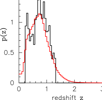
It is important to quantify the effect of the source redshift distribution and of the error in photometric redshifts on the lensing MFs, or indeed on any lensing statistics. We perform ray-tracing simulations by shooting rays to the farthest lens plane at $z=3$, weighting the lensing kernel using a redshift distribution function of the sources. Specifically, we follow the same manner in as Sato et al. (2009) to simulate the weak-lensing effect but the lensing kernel is slightly different from their simulation because of the wider source redshift distribution. In Sato et al. (2009), they assume $z_{p}=1$ so that the lensing kernel can be calculated by the simple expression, i.e., $r(\chi_{s}-\chi_{l})r(\chi_{l})/r(\chi_{s})$, where $\chi_{s}$ and $\chi_{l}$ are the comoving distance of sources and of the lens, respectively. In the present study, we consider source redshift distribution $p(\chi)$. Then the lensing kernel for the lensing objects at $\chi_{l}$ should be replaced with $\int_{\chi_{l}}^{\chi_{H}}{\rm d}\chi_{s}p(\chi_{s})r(\chi_{s}-\chi_{l})r(\chi_{l})/r(\chi_{s})$. The source positions on the sky and all the other characteristics are kept the same as in our original mock catalogs, which themselves are derived from CHFTLenS. For the redshift distribution, we adopt the sum of the posterior PDF of photometric redshift for the galaxies with $0.2<z_{p}<1.3$. Figure 5 compares the integrated redshift distribution with the histograms of the source redshifts. The latter is used in our fiducial simulations. The test data vector ${\mbox{\boldmath$D$}}^{\rm test}$ is calculated by averaging the MFs over the new 40 catalogs with the posterior weight described above.

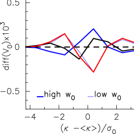
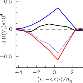
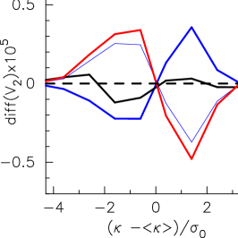
The main difference caused by the different redshift distributions is the amplitude of the standard deviation of ${\cal K}$. We see in Figure 6 that the net difference is as large as those found for cosmological models differing by $\Delta w_{0}=0.2$; this can obviously be a significant source of error in cosmological parameter constraints with upcoming future surveys. We estimate the resulting bias in the derived $w_{0}$ by using Equation (27). The uncertainties in the photometric redshifts can indeed induce a $\Delta w_{0}\sim 0.1$ bias in $w_{0}$. The exact values are summarized in Table 3.

We have also studied the effect of source redshift clustering on the lensing MFs. The results are presented in Appendix A. Briefly, the source redshift clustering is found to be a minor effect, but we note that it could cause non-negligible bias in “precision” cosmology with, for example, the LSST lensing survey.

Shear Calibration Correction

We next study the effect of shear calibration correction. We consider the standard correction that describes the calibration as $\epsilon=(1+m){\mbox{\boldmath$\epsilon$}}_{\rm mock}+{\mbox{\boldmath$c$}}$ with a multiplicative component $m$ and an additive component $c$. The former is calibrated by analyzing simulated images whereas the latter is calibrated empirically using the actual data. An ideal case would be one with $m=c=0$, which might possibly be realized if a perfect calibration is done. We compare the lensing maps with and without the calibration factors $m$ and $c$ in order to quantify the importance of the shear calibration. We simply reanalyze the fiducial mock catalogs by setting $m=c=0$ for all of the source galaxies. The resulting 40 mock catalogs are used to obtain the data vector ${\mbox{\boldmath$D$}}^{\rm test}$ for this study.

We find that the additive calibration induces negligible effect but that the multiplicative calibration affects the lensing MFs appreciably. In the case of CFHTLenS, the multiplicative calibration results in a $\sim 6$ % correction with $\langle 1+m\rangle\simeq 0.94$. Note that $m$ is a function of both the galaxy signal-to-noise ratio and the size. Thus the calibration differs from position to position and introduces effectively additional non-Gaussianities to the ${\cal K}$ map. Figure 6 shows that the non-Gaussianities actually cause biases in the lensing MFs. The biases cannot simply be described by the difference of the standard deviation of ${\cal K}$, i.e., by the normalization of the lensing MFs. The resulting bias in the cosmological parameter estimate is close to the $1\sigma$ level for an HSC-like survey as shown in Table 3. Our study presented here suggests that the multiplicative correction needs to be included in $\it model$ predictions of the MFs for producing robust forecasts for upcoming surveys. We emphasize that our theoretical templates are based on mock catalogs that directly include the multiplicative correction obtained from the real observational data.

Figure 6: Impact of possible systematics on lensing MFs. We plot the differences of average MFs over 40 catalogs between our fiducial cosmology and another one that includes a given systematic. We generate a new set of mock catalogs in order to include systematics in our analysis. The red line shows the difference owing to source redshift distribution whereas the black one represents the effect of shear calibration correction on the lensing MFs. For comparison, the thick (thin) blue line corresponds to the case of a cosmological model with higher (lower) $w_{0}$.

	$\Omega_{\rm m0}$	$A_{s}\times 10^{9}$	$w_{0}$
Redshift distribution	0.00707	-0.0254	-0.122
Calibration correction	-0.0224	0.110	-0.234

Table 3: The bias of cosmological parameter estimation due to possible systematics.

6 APPLICATION to CFHTLenS

We apply all the methods developed and examined in the previous sections to the CFHTLenS data. We have already shown in Section 5.2 that the statistical error in CFHTLenS degrades the constraints on cosmological parameters if we use only the lensing MFs. It would be ideal to utilize other cosmological probes to put tighter constraints. We will use the CMB data from WMAP.

The likelihood analysis in this section includes the systematics studied in Section 5.3, and so our result could be “correctly” biased. Still, the lensing MFs are a powerful cosmological probe, as we shall show in the following.

6.1 Data Sets

We use multiple data sets. As a probe of large-scale structure, we use data from the nine-year WMAP data release (Bennett et al., 2013; Hinshaw et al., 2013). We use the output of Monte Carlo Markov Chains (MCMC) derived from the likelihood analysis with the CMB temperature and polarization power- and cross-spectrum in the WMAP9 data. Note that the MCMC we use here does not include other external data sets, such as small-scale CMB measurements, galaxy redshift surveys, and Hubble constant. We calculate the likelihood in our parameter space $\mbox{\boldmath$p$}=(\Omega_{\rm m0},A_{s},w_{0})$ after marginalizing over the following three parameters: the reionization optical depth $\tau$, scalar spectral index $n_{s}$ and Hubble parameter $H_{0}$.

As a probe of matter distribution at low redshifts, we use the lensing MFs and the 2PCF calculated from the CFHTLenS data. We construct the data vector and covariances in the same manner as in Section 5.1, but we assume no covariances between the MFs and the 2PCF. To validate the assumption, we have actually calculated the parameter constraints by the Fisher analysis with/without covariances between the MFs and the 2PCF. We have found that the approximation does not affect the final results significantly for the current data set. The error in $\Omega_{\rm m0}$ increases only by $\Delta\Omega_{\rm m0}=5\times 10^{-4}$.

We sample the posterior of the cosmological parameters from the lensing 2PCF data set using the Population Monte Carlo (PMC) using the publicly available code ${\tt COSMO\verb|_|PMC}$ (Kilbinger et al., 2011). Details of the PMC are found in Wraith et al. (2009). The method incorporates the cosmological dependence of the shear covariance in the manner described in Eifler et al. (2009). The same model parameters are adopted as in Kilbinger et al. (2013), with the smallest and largest angular bins being 0.9 and 300 arcmin. We consider the following set of cosmological parameters: $\mbox{\boldmath$p$}=({\Omega_{\rm m0},\Omega_{\rm b0},\sigma_{8},H_{0},n_{s},w_{0}})$, where $\Omega_{\rm b0}$ is the baryon density and $\sigma_{8}$ normalizes the matter power spectrum. To compare the result derived from CMB and that from the lensing MFs, we calculate the value of $A_{s}$ at each sample point in parameter space by using the following relation:

$$A_{s} = A_{s,\rm fid}\left(\frac{\sigma_{8}}{\sigma_{8,\rm fid}}\right)^{2}\frac{SD_{+}^{2}|_{\rm fid}}{SD_{+}^{2}},$$ (28)

$$S = \int_{0}^{\infty}\frac{{\rm d}^{3}k}{(2\pi)^{3}}k^{n_{s}}T(k)^{2}|W_{8}(k)|^{2},$$ (29)

where $D_{+}$ is the linear growth factor of matter density, $T(k)$ is the transfer function, and $W_{8}(k)$ is the top-hat function with scale of 8 Mpc/h in the Fourier space. For the fiducial parameter set, we use the same parameters as the WMAP9 best-fit values.

In our PMC run, we perform 30 iterations to find a suitable importance function compared to the posterior. Also 100,000 sample points are generated for each iteration. To obtain a large sample set, we combine the PMC samples with the five highest value of perplexity $p$, which is the conventional diagnostic that indicates the quality and effectiveness of the sampling. Our PMC run achieves $p>0.7$ for the final samples; this criterion is the same as that adopted in the analysis in Kilbinger et al. (2013).

In the next sections, we study the following three cases: (1) likelihood analysis with the lensing MFs alone, (2) combined analysis with the lensing MFs and the 2PCF, and (3) combined analysis with the lensing MFs and CMB anisotropies. In the last analysis, we treat the lensing MFs data and the CMB data as being independent of each other.

6.2 Likelihood Analysis of Lensing MFs

In our maximum likelihood analysis, we assume that the data vector $D$ is well approximated by the multivariate Gaussian distribution with covariance $C$. This assumption is reasonable for the case of joint analysis of the CMB and lensing power spectrum (Sato et al., 2010). In this case, the $\chi^{2}$ statistics (log-likelihood) is given by

$$\chi^{2}=(D_{i}-\mu_{i}({\mbox{\boldmath$p$}}))C^{-1}(D_{j}-\mu_{j}({\mbox{\boldmath$p$}}))$$ (30)

where ${\mbox{\boldmath$\mu$}}({\mbox{\boldmath$p$}})$ is the theoretical prediction as a function of cosmological parameters. The theoretical prediction is computed in a three-dimensional parameter space. In sampling the likelihood function, we consider the limited parameter region as follows: $\Omega_{\rm m0}\in[0,1]$, $A_{s}\times 10^{9}\in[0.1,8.0]$ and $w_{0}\in[-6.5,0.5]$. The sampling number in each parameter is set to 100.

To estimate the MFs components in $\mu$, we assume that the lensing MFs depend linearly on the cosmological parameters with the first derivatives calculated from Equation (24). We consider two components of the contribution of the data covariance in our likelihood analysis; one is the statistical error and sampling variance, which are estimated as in Section 5.1 while the other originates from the possible systematics as studied in Section 5.3. We denote the latter contribution as ${\mbox{\boldmath$C$}}^{\rm sys}$. We estimate ${\mbox{\boldmath$C$}}^{\rm sys}$ in a simple and direct manner using the differences of the MFs, as shown in Figure 6:

$$C^{\rm sys}_{ij}=\left[(D^{\rm zdist}_{i}-D^{\rm fid}_{i})^{2}+(D^{\rm scc}_{i}-D^{\rm fid}_{i})^{2}\right]\delta^{2D}_{ij},$$ (31)

where ${\mbox{\boldmath$D$}}^{\rm fid}$ is the template MFs for our fiducial mock catalogs, ${\mbox{\boldmath$D$}}^{\rm zdist}$ is the average MFs over 40 catalogs reflecting the different source redshift distribution as shown in Figure 5, and ${\mbox{\boldmath$D$}}^{\rm scc}$ is estimated by averaging the MFs over 40 catalogs without shear calibration correction. The total covariance is the sum of the above two contributions.

6.3 Breaking Degeneracies

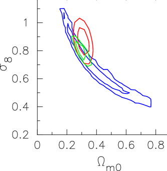
We would like to examine the ability of the lensing MFs to break degeneracies between cosmological parameters. We first consider the concordance $\Lambda$CDM model, i.e. $w_{0}=-1$. Figure 7 shows the marginalized constraints on $\Omega_{\rm 0}$ and $\sigma_{8}$ in the two-parameter plane. Clearly, the lensing MFs can break the well-known degeneracy between $\Omega_{\rm 0}$ and $\sigma_{8}$ that is apparent in the analysis using only the 2PCF. Interestingly, the marginalized constraints on each parameter can be improved by a factor of five to eight by adding the MFs. The final constraints in the case of $\Lambda$CDM model are summarized in Table 4.

	$\Omega_{\rm m0}$	$\sigma_{8}$
2PCF alone	$0.396\pm^{0.177}_{0.185}$	$0.695\pm^{0.203}_{0.202}$
MFs alone	$0.295\pm 0.020$	$0.855\pm^{0.060}_{0.060}$
MFs + 2PCF	$0.282\pm 0.022$	$0.782\pm^{0.042}_{0.042}$

Table 4: Cosmological parameter constraints obtained from the maximum likelihood analysis. The error bar shows the 68% confidence level. The concordance $\Lambda$CDM model is assumed for this pot.

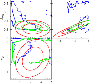
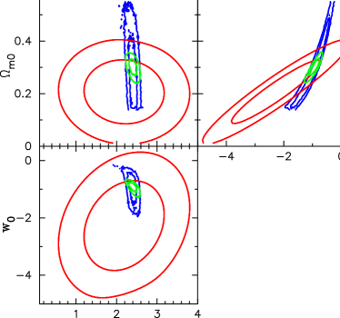
Next, we explore models with a variant of dark energy. The equation of state parameter $w_{0}$ serves as an additional parameter here. The left panel in Figure 8 shows the marginalized constraints in the 2D plane by the lensing MFs and 2PCF. The red circle represents the result from the lensing MFs alone, whereas the green circle is the estimate derived from combining the lensing MFs and 2PCF. Interestingly, with the lensing MFs alone, the data set favors a low $w_{0}$. We have checked that our theoretical MF template can recover correctly the input cosmological parameters for the 40 mock data with a similar confidence level expected from the Fisher analysis. We thus argue that the trend of favoring low $w_{0}$ is likely attributed to the possible systematics as studied in Section 5.3, or to imperfect modeling of the dependence of the lensing MFs on the cosmological parameters.

The right panel of Figure 8 shows the 68% and 95% confidence regions obtained from our joint analysis with the WMAP9 CMB data. The red region represents the results from lensing MFs alone. The blue region is the result obtained from CMB, and the green one represents constraints by combining the both. These figures show clearly that the lensing MFs are useful to improve the cosmological constraints by breaking the parameter degeneracies The marginalized constraints for the three parameters are summarized in Table 5. It is worth making further effort to reduce the systematic errors in measurement of the lensing MFs.

Figure 7: Marginalized 2D confidence level (68% and 95%) obtained from cosmic shear data. The red region represents the cosmological results by lensing MFs alone and the blue region shows the cosmological constraints by 2PCF alone. The green circle shows the result of our combined analysis with the lensing MFs and 2PCF. We assume the concordance $\Lambda$CDM model (i.e., $w_{0}=-1$) for this figure.

Figure 8: Marginalized 2D confidence level (68% and 95%) obtained from the lensing MFs and additional probes. The left panel shows the cosmological constraints by our combined analysis with the lensing MFs and the 2PCF. The right panel shows the result of the joint analysis with the lensing MFs and CMB. In each panel, the red region shows the constraint from the lensing MFs alone and the blue region shows those from the 2PCF or CMB alone. The green one shows the result of the combined analysis with the lensing MFs and another data set.

	$\Omega_{\rm m0}$	$A_{s}\times 10^{9}$	$w_{0}$
MFs alone	$0.205\pm 0.060$	$2.18\pm^{0.60}_{0.60}$	$-2.2\pm 0.8$
MFs + 2PCF	$0.256\pm^{0.054}_{0.046}$	$1.92\pm^{0.65}_{0.65}$	$-1.60\pm^{0.76}_{0.57}$
MFs + CMB	$0.290\pm^{0.016}_{0.028}$	$2.39\pm 0.07$	$-0.90\pm 0.11$

Table 5: We summarize the parameter constraints obtained from the maximum likelihood analysis. The error bar indicates the 68% confidence level.

7 SUMMARY AND CONCLUSION

We have performed mock lensing observations by incorporating the three-dimensional distribution of the source galaxies and the effect of imperfect shape measurement in the same manner as in the analysis of the real CFHTLenS data. We have then used the mock catalogs and performed a Fisher analysis, which yields realistic forecast for constraining $\Omega_{\rm m0}$, $A_{s}$, and $w_{0}$ from the lensing MFs. We have also studied in detail the possible systematics in the lensing MFs measurement that are crucial for cosmological studies. Finally, we have applied the developed method to real cosmic-shear data, to show that the lensing MFs are powerful probe of cosmology.

Our analysis using the CFHTLenS data suggests that the overall statistical error is comparable to the sampling variance for the CHFT survey area and thus the accuracy of cosmological parameter constraints is degraded by a factor of $\sim 2$. Assuming that the statistical error in upcoming wide-field surveys is reduced proportionally to the effective survey area, we find that the lensing MFs can constrain $w_{0}$ with an error of $\Delta w_{0}\sim 0.25$ for HSC survey with a proposed sky coverage of $\sim 1400$ ${\rm deg}^{2}$.

We have clarified the effects of the two major systematics. Because of the uncertainties in photometric redshifts of the source galaxies, the mean redshift of the lens objects is not determined very accurately. We have found that an error of $\Delta z=0.05$ in the mean source redshift results in biased dark energy parameter estimation of $\Delta w_{0}\sim 0.2$ for CFHTLenS. Furthermore, the shear calibration correction causes non-negligible errors that can bias cosmological parameter estimation as large as the 1$\sigma$ confidence level for HSC survey. Clearly, careful studies are needed in order to understand and correct the effects on a survey-by-survey basis.

Weak-lensing MFs are potentially powerful statistics for cosmological studies. They enable us to constrain cosmological models by cosmic-shear observations even without any prior from the cosmic microwave background anisotropies or from the galaxy clustering measurement. There still remain, however, important issues when measuring the MFs from real data set. Although the lensing MFs can be used to extract cosmological information beyond the two-point statistics, the crucial length scales of structure probed are where perturbative approaches break down because of the non-linear gravitational growth (Taruya et al., 2002; Petri et al., 2013). We need accurate theoretical predictions of the lensing MFs beyond perturbation methods (Matsubara, 2003; Munshi et al., 2012) in order to sample accurately likelihood functions for a wide range of cosmological parameters. Another important issue is theoretical uncertainties associated with baryonic effects. Previous studies (e.g., Semboloni et al., 2013; Zentner et al., 2013) explored the effect of including baryonic components to the 2PCFs and consequently to cosmological parameter estimation. The baryonic effect could also be important for the MFs analysis because the MFs generally contain morphological information at arcminute scales, i.e., the typical virial radius of galaxy clusters. Yang et al. (2013) show appreciable baryonic effects on peak statistics using a simple model applied to dark-matter-only simulations. Obviously the most straightforward way to include the baryonic effect would be to perform weak-lensing simulations using outputs of hydrodynamic simulations. We continue studying the MFs along this idea.

There are other possible systematics than those studied in the present paper. For example, source-lens clustering (e.g., Hamana et al., 2002) and the intrinsic alignment (e.g., Hirata & Seljak, 2004) are likely to compromise cosmological parameter estimation. The statistical properties and the correlation of source galaxies and lensing structures are still uncertain but could be critical when making lensing mass maps. A promising approach in theoretical studies would be associating the source positions with their host dark matter halos on the light cone. This is along the line of our ongoing study using a large set of cosmological simulations in combination with actual observations.

Appendix A EFFECT OF SOURCE REDSHIFT CLUSTERING ON THE VARIANCE OF SMOOTHED CONVERGENCE FIELD

Here, we summarize the effect of source redshift clustering on the variance of a smoothed convergence field. Weak-lensing convergence $\kappa$ is given by the integral of matter over density with a weight along the line-of-sight $\theta$:

$$\kappa(\mbox{\boldmath$\theta$},\chi_{s}) = \frac{3}{2}\left(\frac{H_{0}}{c}\right)^{2}\Omega_{\rm m0}\int_{0}^{\chi_{s}}{\rm d}\chi_{\ell}\ g(\chi_{s},\chi_{\ell})\frac{\delta[r(\chi_{\ell})\mbox{\boldmath$\theta$},\chi_{\ell}]}{a(\chi_{\ell})},$$ (A1)

$$g(\chi_{s},\chi_{\ell}) = \frac{r(\chi_{s}-\chi_{\ell})r(\chi_{\ell})}{r(\chi_{s})},$$ (A2)

where $\chi$ is comoving distance, $r(\chi)$ is angular diameter distance, and $\chi_{s}$ represents the comoving distance to a source. One can assign a probability distribution $p(\chi_{s})$ of a source galaxy’s position, or in fact $p(\chi_{s})$ for a population of source galaxies, and integrate as,

$$\bar{\kappa}(\mbox{\boldmath$\theta$})=\frac{3}{2}\left(\frac{H_{0}}{c}\right)^{2}\Omega_{\rm m0}\int_{0}^{\chi_{H}}{\rm d}\chi_{s}\ p(\chi_{s})\int_{0}^{\chi_{s}}{\rm d}\chi_{\ell}\ g(\chi_{s},\chi_{\ell})\frac{\delta[r(\chi_{\ell})\mbox{\boldmath$\theta$},\chi_{\ell}]}{a(\chi_{\ell})}.$$ (A3)

In the conventional multiple lens plane algorithm (White & Hu, 2000; Hamana & Mellier, 2001), one can calculate the both convergence field $\kappa$ and $\bar{\kappa}$ by using a suitable weight function in the integral. In practice in ray-tracing simulations, we shoot rays from the observer point to the source redshifts to obtain $\kappa$, whereas we shoot rays up to some certain (high-)redshift but with weight $p(\chi_{s})$ along the line-of-sights to obtain $\bar{\kappa}$. In the former case, the full three-dimensional positions of the source galaxies are realized as in the observation considered, i.e., CFHTLenS in our case. The difference between $\kappa$ and $\bar{\kappa}$ can be easily seen in a direct manner using the two sets of simulations, and the resulting variances of smoothed convergence field can be explicitly compared.

The smoothed convergence field for $\kappa$ is given by

$${\cal K}(\mbox{\boldmath$\theta$})=\sum_{i}U(\mbox{\boldmath$\theta$}-\mbox{\boldmath$\phi$}_{i})\kappa(\mbox{\boldmath$\phi$}_{i},\chi_{si}),$$ (A4)

where $U(\mbox{\boldmath$\theta$})$ is the filter function for smoothing and the summation is taken over the source objects. The smoothed convergence field for $\bar{\kappa}$ is also obtained in the same way. The two-point correlation function of $\cal{K}$ is then given by

$$\langle{\cal K}(\mbox{\boldmath$\theta$}_{1}){\cal K}(\mbox{\boldmath$\theta$}_{2})\rangle = \langle\sum_{i}\sum_{j}U(\mbox{\boldmath$\theta$}_{1}-\mbox{\boldmath$\phi$}_{i})U(\mbox{\boldmath$\theta$}_{2}-\mbox{\boldmath$\phi$}_{j})\kappa(\mbox{\boldmath$\phi$}_{i},\chi_{si})\kappa(\mbox{\boldmath$\phi$}_{j},\chi_{sj})\rangle$$ (A5)

$$= \int{\rm d}^{2}\phi_{1}{\rm d}^{2}\phi_{2}\,U(\mbox{\boldmath$\theta$}_{1}-\mbox{\boldmath$\phi$}_{1})U(\mbox{\boldmath$\theta$}_{2}-\mbox{\boldmath$\phi$}_{2})$$

$$\times \int{\rm d}\chi_{s1}\,{\rm d}\chi_{s2}\ p(\chi_{s1})p(\chi_{s2})\left[1+\xi_{ss}(\mbox{\boldmath$\phi$}_{1}-\mbox{\boldmath$\phi$}_{2},\chi_{s1},\chi_{s2})\right]$$

$$\hskip 150.0pt\times\langle\kappa(\mbox{\boldmath$\phi$}_{1},\chi_{s1})\kappa(\mbox{\boldmath$\phi$}_{2},\chi_{s2})\rangle,$$

where $\langle\cdots\rangle$ represents the operator of ensemble average and $\xi_{ss}$ represents the two point correlation function of the sources. One can also calculate the two-point correlation of $\bar{\cal K}$ in the similar manner. We then obtain the non-vanishing difference between $\langle\bar{\cal K}\bar{\cal K}\rangle$ and $\langle{\cal K}{\cal K}\rangle$ as

$$\langle\bar{\cal K}\bar{\cal K}-{\cal K}{\cal K}\rangle = \int{\rm d}^{2}\phi_{1}{\rm d}^{2}\phi_{2}\ U(\mbox{\boldmath$\theta$}_{1}-\mbox{\boldmath$\phi$}_{1})U(\mbox{\boldmath$\theta$}_{2}-\mbox{\boldmath$\phi$}_{2})$$ (A6)

$$\times \left[{\bar{\xi}_{ss}}(\mbox{\boldmath$\phi$}_{1}-\mbox{\boldmath$\phi$}_{2})w_{\rm pp}(\mbox{\boldmath$\phi$}_{1}-\mbox{\boldmath$\phi$}_{2})-V_{\rm pp}(\mbox{\boldmath$\phi$}_{1}-\mbox{\boldmath$\phi$}_{2})\right],$$

$$\bar{\xi}_{ss}(\mbox{\boldmath$\phi$}_{1}-\mbox{\boldmath$\phi$}_{2}) = \int{\rm d}\chi_{s1}{\rm d}\chi_{s2}\ p(\chi_{s1})p(\chi_{s2})\xi_{ss}(\mbox{\boldmath$\phi$}_{1}-\mbox{\boldmath$\phi$}_{2},\chi_{s1},\chi_{s2}),$$ (A7)

$$w_{\rm pp}(\mbox{\boldmath$\phi$}_{1}-\mbox{\boldmath$\phi$}_{2}) = \langle\bar{\kappa}(\mbox{\boldmath$\phi$}_{1})\bar{\kappa}(\mbox{\boldmath$\phi$}_{2})\rangle,$$ (A8)

$$V_{\rm pp}(\mbox{\boldmath$\phi$}_{1}-\mbox{\boldmath$\phi$}_{2}) = \frac{9}{4}\left(\frac{H_{0}}{c}\right)^{4}\Omega_{\rm m0}^{2}\int{\rm d}\chi_{s1}{\rm d}\chi_{s2}\ p(\chi_{s1})p(\chi_{s2})\xi_{ss}(\mbox{\boldmath$\phi$}_{1}-\mbox{\boldmath$\phi$}_{2},\chi_{s1},\chi_{s2})$$ (A9)

$$\times \int{\rm d}\chi_{\ell 1}{\rm d}\chi_{\ell 2}\ \frac{g(\chi_{s1},\chi_{\ell 1})g(\chi_{s2},\chi_{\ell 2})}{a(\chi_{\ell 1})a(\chi_{\ell 2})}\langle\delta[r(\chi_{\ell 1})\mbox{\boldmath$\phi_{1}$},\chi_{\ell 1}]\delta[r(\chi_{\ell 2})\mbox{\boldmath$\phi_{2}$},\chi_{\ell 2}]\rangle.$$

This non-vanishing term arises if the source clustering $\xi_{ss}$ evolves over redshift. Note also that the MFs of $\bar{\cal K}$ and those of ${\cal K}$ can be, in general, different if their variances differ (see, e.g. Shirasaki et al., 2013).

In practice, the smoothed convergence field is often estimated from the shear field $\gamma$. In this case, one can calculate ${\cal K}$ using the following equation,

$${\cal K}(\mbox{\boldmath$\theta$})=\sum_{i}Q_{t}(\mbox{\boldmath$\theta$}-\mbox{\boldmath$\phi$}_{i})\gamma_{t}(\mbox{\boldmath$\phi$}_{i},\chi_{si}),$$ (A10)

where $Q_{t}(\mbox{\boldmath$\theta$})$ is the filter function for the shear field which is related to $U(\mbox{\boldmath$\theta$})$ by Equation (16) and $\gamma_{t}(\mbox{\boldmath$\theta$},\chi_{s})$ is the tangential component of shear at the position $\theta$ when a source is at $\chi_{s}$ from the observer. Using Equation (A10), one can derive the correspoding non-vanishing term

$$\langle\bar{\cal K}\bar{\cal K}-{\cal K}{\cal K}\rangle = \int{\rm d}^{2}\phi_{1}{\rm d}^{2}\phi_{2}\ Q_{t}(\mbox{\boldmath$\theta$}_{1}-\mbox{\boldmath$\phi$}_{1})Q_{t}(\mbox{\boldmath$\theta$}_{2}-\mbox{\boldmath$\phi$}_{2})$$ (A11)

$$\times \left[\bar{\xi}_{ss}(\mbox{\boldmath$\phi$}_{1}-\mbox{\boldmath$\phi$}_{2})\langle\bar{\gamma_{t}}(\mbox{\boldmath$\phi$}_{1})\bar{\gamma_{t}}(\mbox{\boldmath$\phi$}_{2})\rangle-V_{\rm pp}^{\gamma}(\mbox{\boldmath$\phi$}_{1}-\mbox{\boldmath$\phi$}_{2})\right],$$

$$V_{\rm pp}^{\gamma}(\mbox{\boldmath$\phi$}_{1}-\mbox{\boldmath$\phi$}_{2}) = \int{\rm d}\chi_{s1}{\rm d}\chi_{s2}\ p(\chi_{s1})p(\chi_{s2})\xi_{ss}(\mbox{\boldmath$\phi$}_{1}-\mbox{\boldmath$\phi$}_{2},\chi_{s1},\chi_{s2})$$ (A12)

$$\times \langle\gamma_{t}(\mbox{\boldmath$\phi$}_{1},\chi_{s1})\gamma_{t}(\mbox{\boldmath$\phi$}_{2},\chi_{s2})\rangle,$$

$$\langle\bar{\gamma_{t}}(\mbox{\boldmath$\phi$}_{1})\bar{\gamma_{t}}(\mbox{\boldmath$\phi$}_{2})\rangle = \frac{9}{4}\left(\frac{H_{0}}{c}\right)^{4}\Omega_{\rm m0}^{2}\int_{0}^{\chi_{H}}\frac{{\rm d\chi}}{a^{2}(\chi)}{\bar{W}}^{2}(\chi)$$ (A13)

$$\times \int\frac{\ell d\ell}{2\pi}P_{\delta}\left(k=\frac{\ell}{r(\chi)},z(\chi)\right)\left(\frac{J_{0}(\ell\phi_{12})+J_{4}(\ell\phi_{12})}{2}\right),$$

$${\bar{W}}(\chi) = \int_{\chi}^{\chi_{H}}{\rm d\chi^{\prime}}p(\chi^{\prime})\frac{r(\chi^{\prime}-\chi)}{r(\chi^{\prime})},$$ (A14)

$$\langle\gamma_{t}(\mbox{\boldmath$\phi$}_{1},\chi_{s1})\gamma_{t}(\mbox{\boldmath$\phi$}_{2},\chi_{s2})\rangle = \frac{9}{4}\left(\frac{H_{0}}{c}\right)^{4}\Omega_{\rm m0}^{2}\int_{0}^{{\rm min}(\chi_{s1},\chi_{s2})}\frac{{\rm d\chi}}{a^{2}(\chi)}\frac{r(\chi_{s1}-\chi)}{r(\chi_{s1})}\frac{r(\chi_{s2}-\chi)}{r(\chi_{s2})}$$ (A15)

$$\times \int\frac{\ell d\ell}{2\pi}P_{\delta}\left(k=\frac{\ell}{r(\chi)},z(\chi)\right)\left(\frac{J_{0}(\ell\phi_{12})+J_{4}(\ell\phi_{12})}{2}\right),$$

where $\phi_{12}$ is the norm of $\mbox{\boldmath$\phi$}_{1}-\mbox{\boldmath$\phi$}_{2}$ and $P_{\delta}(k,z)$ is the non-linear matter power spectrum at redshift $z$.

Figure 9: Impact of a source redshift clustering on lensing MFs. We plot the differences of average MFs over 40 catalogs between our fiducial cosmology and another one that includes a given systematic. We generate a new set of mock catalogs in order to include systematics in our analysis. The red line shows the impact of the difference of source redshift distribution and the green one represents the effect of source redshift clustering on lensing MFs. For comparison, the thick (thin) blue line corresponds to the case of cosmological model with higher (lower) $w_{0}$.

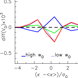
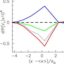
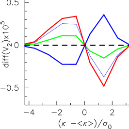
Although we have derived the difference between ${\cal K}$ and ${\bar{\cal K}}$ at the two-point statistics, it is extremely difficult to derive an explicit form for the corresponding difference in the lensing MFs. We thus resort to comparing directly the two sets of simulated lensing MFs. One is our fiducial mock data used in Section 4.2. For the other, new set of simulations, we calculate $\bar{\kappa}$ at each source position on the sky using the source redshift distribution (weight) that is shown as the black histograms in Figure 5. Figure 9 shows the results. The red line shows the difference caused by the two different source redshift distributions as described in Section 5.3. The green line represents the difference of the lensing MFs with and without source redshift clustering. For reference, we also plot the difference of lensing MFs between the different cosmological model by blue lines. The thick (thin) blue lines correspond to the case of the cosmological model with higher (lower) $w_{0}$. Although the impact of source clustering (green) is smaller than the effect of different source distribution (red), it or actually both could be a major source of systematics for future survey with the sky coverage of 20000 ${\rm deg}^{2}$. The induced biases in cosmological parameters due to the source clustering are estimated by Equation (27); the results are $\Delta\Omega_{\rm m0}=0.00642$, $\Delta A_{s}=-0.00467\times 10^{9}$ and $\Delta w_{0}=0.00487$.

Appendix B ESTIMATING THE MINKOWSKI FUNCTIONALS COVARIANCE MATRIX

We describe an approximate way to evaluate the covariance matrix as given by Equation (26) and test its validity in this Appendix. We first generate 40 noise-free lensing maps by the method in Section  4.1. For each realization of the 40 maps, we use a different random seed for the intrinsic ellipticities to make mock source galaxy catalogs described in Section 4.2. In this way, we generate $40\times 40=1600$ catalogs in total, which can be used to estimate the full covariance of the MFs.

	$x_{1}$	$x_{2}$	$x_{3}$	$x_{4}$	$x_{5}$
$x_{1}$	1.96	0.35	1.96	4.07	1.87
$x_{2}$		1.53	1.51	1.27	1.46
$x_{3}$			1.82	2.12	1.92
$x_{4}$				1.14	0.98
$x_{5}$					1.82

Table 6: The ratio of the full covariance of $V_{0}$ to our estimator. The full covariance is derived from the new 1600 maps with Equation (B1), whereas our estimator is given by Equation (B3).

Let us denote a mock catalogue as ${\cal K}^{m,n}$, which is generated by the $m$th noise free lensing map with an $n$th random seed of the intrinsic ellipticity distribution. We then calculate the full covariance of $V_{0}$ as follows:

$$C^{(40,40)}_{ij} \equiv \frac{1}{1600-1}\sum_{m=1}^{40}\sum_{n=1}^{40}\sum_{i,j}(V_{0}(x^{m,n}_{i})-\bar{V}_{0}(x^{m,n}_{i}))(V_{0}(x^{m,n}_{j})-\bar{V}_{0}(x^{m,n}_{j})),$$ (B1)

$$\bar{V}_{0}(x^{m,n}_{i}) \equiv \frac{1}{1600}\sum_{m=1}^{40}\sum_{n=1}^{40}V_{0}(x^{m,n}_{i}),$$ (B2)

where $x^{m,n}_{i}=({\cal K}_{i}^{m,n}-\langle{\cal K}^{m,n}\rangle)/\sigma_{0}^{m,n}$ and we here use five bins in the range of $x_{i}=[-3:3]$. We also calculate our estimator adopted in this paper:

$$C_{ij} = C^{(40,1)}_{ij}+C^{(1,40)}_{ij},$$ (B3)

where

$$C^{(1,40)}_{ij} \equiv \frac{1}{40-1}\sum_{n=1}^{40}\sum_{i,j}(V_{0}(x^{1,n}_{i})-\bar{V}_{0}(x^{1,n}_{i}))(V_{0}(x^{1,n}_{j})-\bar{V}_{0}(x^{1,n}_{j})),$$ (B4)

$$C^{(40,1)}_{ij} \equiv \frac{1}{40-1}\sum_{m=1}^{40}\sum_{i,j}(V_{0}(x^{m,1}_{i})-\bar{V}_{0}(x^{m,1}_{i}))(V_{0}(x^{m,1}_{j})-\bar{V}_{0}(x^{m,1}_{j})),$$ (B5)

$$\bar{V}_{0}(x^{1,n}_{i}) \equiv \frac{1}{40}\sum_{n=1}^{40}V_{0}(x^{1,n}_{i}),$$ (B6)

$$\bar{V}_{0}(x^{m,1}_{i}) \equiv \frac{1}{40}\sum_{m=1}^{40}V_{0}(x^{m,1}_{i}).$$ (B7)

The ratio $C^{(40,40)}_{ij}/C_{ij}$ then serves a check on the accuracy of our estimator. We summarize the ratio for each component in Table 6. Our estimator indeed gives a good approximation to the full covariance. The ratio is typically within a factor of two, and the same is also found for $V_{1}$ and $V_{2}$. Even if the ratio of the full covariance and our estimator is 2 for all the matrix elements, the cosmological forecast shown in this paper would be degraded only by a factor of $\sim 2^{1/3}$ (i.e., $\sim 20\%$).

References

- Bartelmann & Schneider (2001) Bartelmann, M., & Schneider, P. 2001, Phys.Rept., 340, 291
- Benítez (2000) Benítez, N. 2000, ApJ, 536, 571
- Benjamin et al. (2013) Benjamin, J., Van Waerbeke, L., Heymans, C., et al. 2013, MNRAS, 431, 1547
- Bennett et al. (2013) Bennett, C. L., Larson, D., Weiland, J. L., et al. 2013, ApJS, 208, 20
- Bolzonella et al. (2000) Bolzonella, M., Miralles, J.-M., & Pelló, R. 2000, A&A, 363, 476
- Crocce et al. (2006) Crocce, M., Pueblas, S., & Scoccimarro, R. 2006, MNRAS, 373, 369
- Eifler et al. (2009) Eifler, T., Schneider, P., & Hartlap, J. 2009, A&A, 502, 721
- Erben et al. (2001) Erben, T., Van Waerbeke, L., Bertin, E., Mellier, Y., & Schneider, P. 2001, A&A, 366, 717
- Erben et al. (2013) Erben, T., Hildebrandt, H., Miller, L., et al. 2013, MNRAS, 433, 2545
- Hamana et al. (2002) Hamana, T., Colombi, S. T., Thion, A., et al. 2002, MNRAS, 330, 365
- Hamana & Mellier (2001) Hamana, T., & Mellier, Y. 2001, MNRAS, 327, 169
- Hamana et al. (2004) Hamana, T., Takada, M., & Yoshida, N. 2004, MNRAS, 350, 893
- Hartlap et al. (2007) Hartlap, J., Simon, P., & Schneider, P. 2007, A&A, 464, 399
- Heymans et al. (2012) Heymans, C., Van Waerbeke, L., Miller, L., et al. 2012, MNRAS, 427, 146
- Hikage et al. (2011) Hikage, C., Takada, M., Hamana, T., & Spergel, D. 2011, MNRAS, 412, 65
- Hildebrandt et al. (2012) Hildebrandt, H., Erben, T., Kuijken, K., et al. 2012, MNRAS, 421, 2355
- Hinshaw et al. (2013) Hinshaw, G., Larson, D., Komatsu, E., et al. 2013, ApJS, 208, 19
- Hirata & Seljak (2003) Hirata, C., & Seljak, U. 2003, MNRAS, 343, 459
- Hirata & Seljak (2004) Hirata, C. M., & Seljak, U. 2004, Phys. Rev. D, 70, 063526
- Huterer et al. (2006) Huterer, D., Takada, M., Bernstein, G., & Jain, B. 2006, MNRAS, 366, 101
- Kaiser (1992) Kaiser, N. 1992, Astrophys.J., 388, 272
- Kaiser (2000) Kaiser, N. 2000, ApJ, 537, 555
- Kilbinger et al. (2011) Kilbinger, M., Benabed, K., Cappe, O., et al. 2011, ArXiv e-prints
- Kilbinger et al. (2013) Kilbinger, M., Fu, L., Heymans, C., et al. 2013, MNRAS, 430, 2200
- Komatsu et al. (2011) Komatsu, E., Smith, K. M., Dunkley, J., et al. 2011, ApJS, 192, 18
- Kratochvil et al. (2012) Kratochvil, J. M., Lim, E. A., Wang, S., et al. 2012, Phys. Rev. D, 85, 103513
- Lewis et al. (2000) Lewis, A., Challinor, A., & Lasenby, A. 2000, Astrophys. J., 538, 473
- Lim & Simon (2012) Lim, E. A., & Simon, D. 2012, J. Cosmology Astropart. Phys, 1, 48
- Limber (1954) Limber, D. N. 1954, Astrophys.J., 119, 655
- Mandelbaum et al. (2013) Mandelbaum, R., Slosar, A., Baldauf, T., et al. 2013, MNRAS, 432, 1544
- Matsubara (2003) Matsubara, T. 2003, ApJ, 584, 1
- Matsubara & Jain (2001) Matsubara, T., & Jain, B. 2001, ApJ, 552, L89
- Miller et al. (2013) Miller, L., Heymans, C., Kitching, T. D., et al. 2013, MNRAS, 429, 2858
- Munshi et al. (2008) Munshi, D., Valageas, P., Van Waerbeke, L., & Heavens, A. 2008, Phys.Rept., 462, 67
- Munshi et al. (2012) Munshi, D., van Waerbeke, L., Smidt, J., & Coles, P. 2012, MNRAS, 419, 536
- Nishimichi et al. (2009) Nishimichi, T., Shirata, A., Taruya, A., et al. 2009, PASJ, 61, 321
- Petri et al. (2013) Petri, A., Haiman, Z., Hui, L., May, M., & Kratochvil, J. M. 2013, Phys. Rev. D, 88, 123002
- Reid et al. (2010) Reid, B. A., Percival, W. J., Eisenstein, D. J., et al. 2010, MNRAS, 404, 60
- Sato et al. (2001) Sato, J., Takada, M., Jing, Y. P., & Futamase, T. 2001, ApJ, 551, L5
- Sato et al. (2009) Sato, M., Hamana, T., Takahashi, R., et al. 2009, ApJ, 701, 945
- Sato et al. (2010) Sato, M., Ichiki, K., & Takeuchi, T. T. 2010, Physical Review Letters, 105, 251301
- Schneider et al. (2002) Schneider, P., van Waerbeke, L., Kilbinger, M., & Mellier, Y. 2002, A&A, 396, 1
- Seitz & Schneider (1997) Seitz, C., & Schneider, P. 1997, A&A, 318, 687
- Semboloni et al. (2013) Semboloni, E., Hoekstra, H., & Schaye, J. 2013, MNRAS, 434, 148
- Shirasaki et al. (2013) Shirasaki, M., Yoshida, N., & Hamana, T. 2013, ApJ, 774, 111
- Shirasaki et al. (2012) Shirasaki, M., Yoshida, N., Hamana, T., & Nishimichi, T. 2012, ApJ, 760, 45
- Spergel et al. (2007) Spergel, D. N., Bean, R., Doré, O., et al. 2007, ApJS, 170, 377
- Springel (2005) Springel, V. 2005, MNRAS, 364, 1105
- Takahashi et al. (2012) Takahashi, R., Sato, M., Nishimichi, T., Taruya, A., & Oguri, M. 2012, ApJ, 761, 152
- Taruya et al. (2002) Taruya, A., Takada, M., Hamana, T., Kayo, I., & Futamase, T. 2002, ApJ, 571, 638
- Tegmark et al. (2006) Tegmark, M., Eisenstein, D. J., Strauss, M. A., et al. 2006, Phys. Rev. D, 74, 123507
- Valageas & Nishimichi (2011) Valageas, P., & Nishimichi, T. 2011, A&A, 527, A87
- Van Waerbeke et al. (2013) Van Waerbeke, L., Benjamin, J., Erben, T., et al. 2013, MNRAS, 433, 3373
- White & Hu (2000) White, M., & Hu, W. 2000, ApJ, 537, 1
- Wraith et al. (2009) Wraith, D., Kilbinger, M., Benabed, K., et al. 2009, Phys. Rev. D, 80, 023507
- Yang et al. (2013) Yang, X., Kratochvil, J. M., Huffenberger, K., Haiman, Z., & May, M. 2013, Phys. Rev. D, 87, 023511
- Zentner et al. (2013) Zentner, A. R., Semboloni, E., Dodelson, S., et al. 2013, Phys. Rev. D, 87, 043509