Contextually Supervised Source Separation with Application to Energy Disaggregation

Abstract

We propose a new framework for single-channel source separation that lies between the fully supervised and unsupervised setting. Instead of supervision, we provide input features for each source signal and use convex methods to estimate the correlations between these features and the unobserved signal decomposition. We analyze the case of $\ell_{2}$ loss theoretically and show that recovery of the signal components depends only on cross-correlation between features for different signals, not on correlations between features for the same signal. Contextually supervised source separation is a natural fit for domains with large amounts of data but no explicit supervision; our motivating application is energy disaggregation of hourly smart meter data (the separation of whole-home power signals into different energy uses). Here we apply contextual supervision to disaggregate the energy usage of thousands homes over four years, a significantly larger scale than previously published efforts, and demonstrate on synthetic data that our method outperforms the unsupervised approach.

1 Introduction

We consider the single-channel source separation problem, in which we wish to separate a single aggregate signal into mixture of unobserved component signals. Traditionally, this problem has been approached in two ways: the supervised setting [11, 17, 18], where we have access to training data with the true signal separations and the unsupervised (or “blind”) setting [3, 6, 13, 19], where we have only the aggregate signal. However, both settings have potential drawbacks: for many problems, including energy disaggregation—which looks to separate individual energy uses from a whole-home power signal [9]—it can be difficult to obtain training data with the true separated signals needed for the supervised setting; in contrast, the unsupervised setting is an ill-defined problem with arbitrarily many solutions, and thus algorithms are highly task-dependent.

In this work, we propose an alternative approach that lies between these two extremes. We propose a framework of contextual supervision, whereby along with the input signal to be separated, we provide contextual features correlated with the unobserved component signals. In practice, we find that this is often much easier than providing a fully supervised training set; yet it also allows for a well-defined problem, unlike the unsupervised setting. The approach is a natural fit for energy disaggregation, since we have strong correlations between energy usage and easily observed context—air conditioning spikes in hot summer months, lighting increases when there is a lack of sunlight, etc. We formulate our model directly as an optimization problem in which we jointly estimate these correlations along with the most likely source separation. Theoretically, we show that when the contextual features are relatively uncorrelated between different groups, we can recover the correct separation with high probability. We demonstrate that our model recovers the correct separation on synthetic examples resembling the energy disaggregation task and apply the method to the task of separating sources of energy usage for thousands of homes over 4 years, a scale much larger than previously published efforts. The main contributions of this paper are 1) the proposed contextually supervised setting and the optimization formulation; 2) the theoretical analysis showing that accurate separation only requires linear independence between features for different signals; and 3) the application of this approach to the problem of energy disaggregation, a task with significant potential to help inform consumers about their energy behavior, thereby increasing efficiency.

2 Related work

As mentioned above, work in single-channel source separation has been separated along the lines of supervised and unsupervised algorithms, although several algorithms can be applied to either setting. A common strategy is to separate the observed aggregate signal into a linear combination of several bases, where different bases correspond to different components of the signal; algorithms such as Probabilistic Latent Component Analysis (PLCA) [20], sparse coding [15], and factorial hidden Markov models (FHMMs) [8] all fall within this category, with the differences concerning 1) how bases are represented and assigned to different signal components and 2) how the algorithm infers the activation of the different bases given the aggregate signal. For example, PLCA typically uses pre-defined basis functions (commonly Fourier or Wavelet bases), with a probabilistic model for how sources generate different bases; sparse coding learns bases tuned to data while encouraging sparse activations; and FHMMs use hidden Markov models to represent each source. In the supervised setting, one typically uses the individual signals to learn parameters for each set of bases (e.g., PLCA will learn which bases are typical for each signal), whereas unsupervised methods learn through an EM-like procedure or by maximizing some separation criteria for the learned bases. The method we propose here is conceptually similar, but the nature of these bases is rather different: instead of fixed bases with changing activations, we require features that effectively generate time-varying bases and learn activations that are constant over time.

Orthogonal to this research, there has also been a great deal of work in multi-channel blind source separation problems, where we observe multiple mixings of the same sources (typically, as many mixings as there are signals) rather than in isolation. These methods can exploit significantly more structure and algorithms like Independent Component Analysis [4, 2] can separate signals with virtually no supervised information. However, when applied to the single-channel problem (when this is even possible), they typically perform substantially worse than methods which exploit structure in the problem, such as those described above.

From the applied point of view, algorithms for energy disaggregation have received growing interest in recently years [11, 22, 12, 16]. This is an important task since many studies have shown that consumers naturally adopt energy conserving behaviors when presented with a breakdown of their energy usage [5, 14, 7]. Algorithmic approaches to disaggregation are appealing as they allow for these types of breakdowns, but existing disaggregation approaches virtually all use high-frequency sampling of the whole-building power signal (e.g. per second) requiring the installation of custom monitoring hardware for data collection. In contrast, this work focuses on disaggregation using data from “smart meters”, communication-enabled power meters that are currently installed in more than 32 million homes [21], but are limited to recording usage at low frequencies (every 15 minutes or hour), leading to a substantially different set of challenges. Smart meters are relatively new and deployment is ongoing, but due to the large amount of data available now and in the near future, successful disaggregation has the potential to have a profound impact on energy efficiency.

3 Optimization Formulation

We begin by formulating the optimization problem for contextual source separation. Formally, we assume there is some unknown matrix of $k$ component signals

$$Y\in\mathbb{R}^{T\times k}=\left[\begin{array}[]{cccc}\mid&\mid&&\mid\\ y_{1}&y_{2}&\cdots&y_{k}\\ \mid&\mid&&\mid\end{array}\right]$$ (1)

from which we observe the sum $\bar{y}=\sum_{i=1}^{k}y_{i}$. For example, in our disaggregation setting, $y_{i}\in\mathbb{R}^{T}$ could denote a power trace (with $T$ total readings) for a single type of appliance, such as the air conditioning, lighting, or electronics, and $\bar{y}$ denotes the sum of all these power signals, which we observe from a home’s power meter.

In our proposed model, we represent each individual component signal $y_{i}$ as a linear function of some component-specific bases $X_{i}\in\mathbb{R}^{T\times n_{i}}$

$$y_{i}\approx X_{i}\theta_{i}$$ (2)

where $\theta_{i}\in\mathbb{R}^{n_{i}}$ are the signal’s coefficients. The formal objective of our algorithm is: given the aggregate signal $\bar{y}$ and the component features $X_{i}$, $i=1,\ldots,k$, estimate both the parameters $\theta_{i}$ and the unknown source components $y_{i}$. We cast this as an optimization problem

$$\begin{split}\operatorname*{minimize}_{Y,\theta}\;\;&\sum_{i=1}^{k}\left\{\ell_{i}(y_{i},X_{i}\theta_{i})+g_{i}(y_{i})+h_{i}(\theta_{i})\right\}\\ \operatorname*{subject\;to}\;\;&\sum_{i=1}^{k}y_{i}=\bar{y}\\ \end{split}$$ (3)

where $\ell_{i}:\mathbb{R}^{T}\times\mathbb{R}^{T}\rightarrow\mathbb{R}$ is a loss function penalizing differences between the $i$th reconstructed signal and its linear representation; $g_{i}$ is a regularization term encoding the “likely” form of the signal $y_{i}$, independent of the features; and $h_{i}$ is a regularization penalty on $\theta_{i}$. Choosing $\ell_{i}$, $g_{i}$ and $h_{i}$ to be convex functions results in a convex optimization problem.

A natural choice of loss function $\ell_{i}$ is a norm penalizing the difference between the reconstructed signal and its features $\|y_{i}-X_{i}\theta_{i}\|$, but since our formulation enables loss functions that depend simultaneously on all $T$ values of the signal, we allow for more complex choices as well. For example in the energy disaggregation problem, air conditioning is correlated with high temperature but does not respond to outside temperature changes instantaneously; thermal mass and the varying occupancy in buildings often results in air conditioning usage that correlates with high temperature over some window (for instance, if no one is in a room during a period of high temperature, we may not use electricity then, but need to “make up” for this later when someone does enter the room). Thus, the loss function

$$\ell_{i}(y_{i},X_{i}\theta_{i})=\|(y_{i}-X_{i}\theta_{i})(I\otimes 1^{T})\|^{2}_{2}$$ (4)

which penalizes the aggregate difference of $y_{i}$ and $X_{i}\theta_{i}$ over a sliding window, can be used to capture such dynamics. In many settings, it may also make sense to use $\ell_{1}$ or $\ell_{\infty}$ rather than $\ell_{2}$ loss, depending on the nature of the source signal.

Likewise, since the objective term $g_{i}$ depends on all $T$ values of $y_{i}$, we can use it to encode the likely dynamics of the source signal independent of $X_{i}\theta_{i}$. For air conditioning and other single appliance types, we expect transitions between on/off states which we can encode by penalizing the $\ell_{1}$ norm of $Dy_{i}$ where $D$ is the linear difference operator subtracting $(y_{i})_{t-1}-(y_{i})_{t}$. For other types of energy consumption, for example groups of many electronic appliances, we expect the signal to have smoother dynamics and thus $\ell_{2}$ loss is more appropriate. Finally, we also include $h_{i}$ for statistical regularization purposes—but for problems where $T\gg n_{i}$, such as the ones we consider in our experiments, the choice of $h_{i}$ is less important.

4 Theoretical analysis

Next, we consider the ability of our model to recover the true source signals as $T$ grows while $k$ and $n_{i}$ remain fixed. For the purposes of this section only, we restrict our attention to the choice of $\ell_{2}$ loss, no $g_{i}$ or $h_{i}$ terms, and Gaussian noise (the extension to the sub-Gaussian case is straightforward). We show that under this specialization of the model, the optimization problem recovers the underlying signals at a rate dependent on the linear independence between blocks of input features $X_{i}$. In practice, the choice of $\ell_{i}$, $g_{i}$ and $h_{i}$ is problem-specific, but $\ell_{2}$ loss is a reasonable default and while simplifying the theoretical analysis dramatically, captures the essential behavior of the model in the large $T$ regime.

Formally, for this section we assume the source signals have Gaussian noise

$$y_{i}=X_{i}\theta^{\star}_{i}+w_{i}$$ (5)

for some $\theta^{\star}_{i}\in\mathbb{R}^{n_{i}}$ and $w_{i}\sim\mathcal{N}(0,\sigma_{i}^{2}I)$. Under the choice of $\ell_{2}$ loss, our optimization problem simplifies to

$$\begin{split}\operatorname*{minimize}_{Y,\theta}\;\;&\|Y1-X\theta\|_{2}^{2}\\ \operatorname*{subject\;to}\;\;&Y1=\bar{y}\end{split}$$ (6)

where $1\in\mathbb{R}^{k}$ is the all-ones vector, $\theta\in\mathbb{R}^{n}$ is a concatenation of all the $\theta_{i}$’s, $X\in\mathbb{R}^{T\times n}$ is a concatenation of all the $X_{i}$’s and $n=\sum_{i=1}^{k}n_{i}$ is the total number of features. In particular, estimation of $\theta$ is equivalent to least-squares

$$\hat{\theta}\in\mathbb{R}^{n}=\arg\min_{\theta}\|\bar{y}-X\theta\|_{2}^{2}=(X^{T}X)^{-1}X^{T}{\bar{y}}.$$ (7)

Since each $y_{i}$ has it’s own noise term, we can never expect to recover $y_{i}$ exactly, but we can recover the true $\theta^{\star}$ with analysis that is the same as for standard linear regression. However, in the context of source separation, we are interested in the recovery of the “noiseless” $y_{i}$, $X_{i}\theta^{\star}_{i}$, and thus in our analysis we consider how the root mean squared error

$$\mathrm{RMSE}(X_{i}\hat{\theta}_{i})=\sqrt{\frac{1}{T}\left\|X_{i}\hat{\theta}_{i}-X_{i}\theta_{i}^{\star}\right\|_{2}^{2}}$$ (8)

vanishes for large $T$; indeed, a key feature of our analysis is to show that we may recover the underlying signals faster than $\theta^{\star}_{i}$.

Theorem 1.

Given data generated by the model (5), and estimating $\hat{\theta}$ via (7), we have that

$$\mathbf{E}\left[\|X_{i}\hat{\theta}_{i}-X_{i}\theta^{\star}\|_{2}^{2}\right]=\sigma^{2}\operatorname*{tr}X_{i}^{T}X_{i}(X^{T}X)^{-1}_{ii}\leq\sigma^{2}n_{i}\rho_{i}$$ (9)

where $\sigma^{2}=\sum_{i=1}^{k}\sigma_{i}^{2}$ and $\rho_{i}=\lambda_{\max}(X_{i}^{T}X_{i}(X^{T}X)^{-1}_{ii})$. Furthermore, for $\delta\leq 0.1$, with probability greater than $1-\delta$

$$\mathrm{RMSE}(X_{i}\hat{\theta}_{i})\leq\sqrt{\frac{4\sigma^{2}n_{i}\rho_{i}\log(1/\delta)}{T}}.$$ (10)

A key quantity in this theorem is the matrix $X_{i}^{T}X_{i}(X^{T}X)^{-1}_{ii}\in\mathbb{R}^{n_{i}\times n_{i}}$; $(X^{T}X)^{-1}_{ii}$ denotes the $i,i$ block of the full inverse $(X^{T}X)^{-1}$ (i.e., first inverting the joint covariance matrix of all the features, and then taking the $i,i$ block), and this term provides a measure of the linear independence between features corresponding to different signals. To see this, note that if features across different signals are orthogonal, $X^{T}X$ is block diagonal, and thus $X_{i}^{T}X_{i}(X^{T}X)^{-1}_{ii}=X_{i}^{T}X_{i}(X_{i}^{T}X_{i})^{-1}=I$, so $\rho_{i}=1$. Alternatively, if two features provided for different signals are highly correlated, entries of $(X^{T}X)_{ii}^{-1}$ will have large magnitude that is not canceled by $X_{i}^{T}X_{i}$ and $\rho_{i}$ will be large. This formalizes an intuitive notion for contextually supervised source separation: for recovering the underlying signals, it does not matter if two features for the same signal are highly correlated (this contrasts to the case of recovering $\theta^{\star}$ itself which depends on all correlations), but two correlated signals for different features make estimation difficult; intuitively, if two very similar features are provided for two different source signals, attribution becomes difficult. A particularly useful property of these bounds is that all terms can be computed using just $X_{i}$, so we can estimate recovery rates when choosing our design matrix.

4.1 Proofs

The proof of Theorem 1 proceeds in two steps. First, using rules for linear transformations of Gaussian random variables, we show that the quantity $X_{i}(\hat{\theta}_{i}-\theta^{\star}_{i})$ is also (zero-mean) Gaussian, which immediately leads to (9). Second, we derive a tail bound on the probability that $X_{i}(\hat{\theta}_{i}-\theta^{\star}_{i})$ exceeds some threshold, which leads to the sample complexity bound (10); because this quantity has a singular covariance matrix, this requires a slightly specialized probability bound, given by the following lemma.

Lemma 1.

Suppose $x\in\mathbb{R}^{p}\sim\mathcal{N}(0,\Sigma)$ with $\mathrm{rank}(\Sigma)=n$. Then

$$P\left(\|x\|_{2}^{2}\geq t\right)\leq\left(\frac{t}{n\lambda}\right)^{n/2}\exp\left\{-\frac{1}{2}(t/\lambda-n)\right\}$$ (11)

where $\lambda$ is the largest eigenvalue of $\Sigma$.

Proof.

By Chernoff’s bound

$$P\left(\|x\|_{2}^{2}\geq t\right)\leq\frac{\mathbf{E}\left[e^{\alpha\|x\|_{2}^{2}}\right]}{e^{\alpha t}}.$$ (12)

for any $\alpha\geq 0$. For any $\epsilon>0$, $z\sim\mathcal{N}(0,\Sigma+\epsilon I)$,

$$\begin{split}\mathbf{E}\left[e^{\alpha\|z\|_{2}^{2}}\right]&=(2\pi)^{-p/2}|\Sigma+\epsilon I|^{-1/2}\int\exp\left\{-\frac{1}{2}z^{T}(\Sigma+\epsilon I)^{-1}z+\alpha z^{T}z\right\}dz\\ &=(2\pi)^{-p/2}|\Sigma+\epsilon I|^{-1/2}\int\exp\left\{-\frac{1}{2}z^{T}(\Sigma+\epsilon I)^{-1}(I-2\alpha(\Sigma+\epsilon I)^{-1})z\right\}dz\\ &=(2\pi)^{-p/2}|\Sigma+\epsilon I|^{-1/2}(2\pi)^{p/2}|\Sigma+\epsilon I|^{1/2}|I-2\alpha(\Sigma+\epsilon I)|^{-1/2}\end{split}$$ (13)

so taking the limit $\epsilon\rightarrow 0$, we have that $\mathbf{E}[e^{\alpha\|x\|_{2}^{2}}]=|I-2\alpha\Sigma|^{-1/2}$. Since $\Sigma$ has only $n$ nonzero eigenvalues,

$$|I-2\alpha\Sigma|=\prod_{i=1}^{n}(1-2\alpha\lambda_{i})\geq(1-2\alpha\lambda)^{n}$$ (14)

and so

$$P\left(\|x\|_{2}^{2}\geq t\right)\leq\frac{1}{(1-2\alpha\lambda)^{n/2}e^{\alpha t}}.$$ (15)

Minimizing this expression over $\alpha$ gives $\alpha=\frac{t-n\lambda}{2t\lambda}$ and substituting this into the equation above gives the desired bound. ∎

To write the problem more compactly, we define the block matrix $W\in\mathbb{R}^{T\times k}$ with columns $w_{i}$, and define the “block-diagonalization” operator $B:\mathbb{R}^{n}\rightarrow\mathbb{R}^{n\times k}$ as

$$B(\theta)=\left[\begin{array}[]{cccc}\theta_{1}&0&\cdots&0\\ 0&\theta_{2}&\cdots&0\\ \vdots&\vdots&\ddots&\vdots\\ 0&0&\cdots&\theta_{k}\end{array}\right].$$ (16)

Proof.

(of Theorem 1) Since $Y=XB(\theta^{\star})+W$,

$$\begin{split}XB(\hat{\theta})&=XB\left((X^{T}X)^{-1}X^{T}(XB(\theta^{\star})+W)1\right)\\ &=XB(B(\theta^{\star}))1+XB\left((X^{T}X)^{-1}X^{T}W1\right)\\ &=XB(\theta^{\star})+XB\left((X^{T}X)^{-1}X^{T}W1\right)\end{split}$$ (17)

For simplicity of notation we also denote

$$u\in\mathbb{R}^{n}\equiv(X^{T}X)^{-1}X^{T}W1.$$ (18)

Thus

$$XB(\theta^{\star})-XB(\hat{\theta})=XB(u).$$ (19)

Now, using rules for Gaussian random variables under linear transformations $W1\sim\mathcal{N}(0,\sigma^{2}I_{T})$ and so $u\sim\mathcal{N}(0,\sigma^{2}(X^{T}X)^{-1})$. Finally, partioning $u_{1},u_{2},\ldots,u_{k}$ conformally with $\theta$,

$$X_{i}\theta^{\star}-X_{i}\hat{\theta}_{i}=X_{i}u_{i}\sim\mathcal{N}(0,\sigma^{2}X_{i}(X^{T}X)^{-1}_{ii}X_{i}^{T})$$ (20)

so

$$\mathbf{E}\left[\left\|X_{i}\theta^{\star}-X_{i}\hat{\theta}_{i}\right\|_{2}^{2}\right]=\sigma^{2}\operatorname*{tr}X_{i}^{T}X_{i}(X^{T}X)^{-1}_{ii}.$$ (21)

Since $\sigma^{2}X_{i}(X^{T}X)^{-1}_{ii}X_{i}^{T}$ is a rank $n_{i}$ matrix with maximum eigenvalue equal to $\sigma^{2}\rho_{i}$, applying Lemma 1 above gives

$$P\left(\mathrm{RMSE}(X_{i}\hat{\theta}_{i})\geq\epsilon\right)=P\left(\|X_{i}u_{i}\|^{2}_{2}\geq T\epsilon^{2}\right)\leq\left(\frac{T\epsilon^{2}}{n_{i}\sigma^{2}\rho_{i}}\right)^{n_{i}/2}\exp\left\{-\frac{1}{2}\left(\frac{T\epsilon^{2}}{\sigma^{2}\rho_{i}}-n_{i}\right)\right\}.$$ (22)

Setting the right hand side equal to $\delta$ and solving for $\epsilon$ gives

$$\epsilon=\sqrt{\frac{-W(-\delta^{2/n}/e)n_{i}\rho_{i}\sigma^{2}}{T}}$$ (23)

where $W$ denotes the Lambert $W$ function (the inverse of $f(x)=xe^{x}$). The theorem follows by noting that $-W(-\delta^{2/n}/e)\leq 4\log\frac{1}{\delta}$ for all $n\geq 1$ when $\delta\leq 0.1$, with both quantities always positive in this range (note that leaving the $W$ term in the bound can be substantially tighter in some cases). ∎

5 Experimental results

Figure 1: Comparing 100 random experiments with the theoretical mean and 90% upper bound for increasing $T$ (left); fixing $T=500$ and varying $\rho_{i}$ (center); and compared to the recovery of $\theta_{1}$ directly (right).

In this section we evaluate contextual supervision on synthetic data and apply in to disaggregate smart meter data collected from thousands of homes. Since labeled data is unavailable, we design a synthetic disaggregation task similar to energy disaggregation from smart meters in order to evaluate our performance on this task quantitatively. Here we explore the choice of loss functions and demonstrate that contextual supervision dramatically outperforms the unsupervised approach.

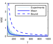
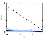
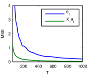
Rates for signal recovery. We begin with a set of experiments examining the ability of the model to recover the underlying source signals as predicted by our theoretical analysis. In these experiments, we consider the problem of separating two source signals with $X_{i}\in\mathbb{R}^{T\times 16}$ sampled independently from a zero-mean Normal with covariance $I+(1-\mu)11^{T}$; we sample $\theta_{i}^{\star}$ uniformly from $[-1,1]$ and $Y\sim\mathcal{N}(X\theta^{\star},I)$. Setting $\mu=0.01$ causes the features for each signal to be highly correlated with each other but since $X_{i}$ are sampled independently, not highly correlated across signals. In Figure 1, we see that MSE vanishes as $T$ grows; when comparing these experimental results to the theoretical mean and 90% upper bound, we see that at least in these experiments, the bound is somewhat loose for large values of $\rho_{i}$. We are also able to recover $\theta^{\star}$ (which is expected since the least-squares estimator $\hat{\theta}$ is consistent), but the rate is much slower due to high correlations in $X_{i}$.

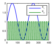
Disaggregation of synthetic data. The next set of experiments considers a synthetic generation process that more closely mimics signals that we encounter in energy disaggregation. The process described visually in Figure 2 (top) begins with two signals, the first is smoothly varying over time while the other is a repeating step function

$$X_{1}(t)=\sin(2\pi t/\tau_{1})+1,\quad X_{2}(t)=I(t\bmod\tau_{2}<\tau_{2}/2)$$ (24)

where $I(\cdot)$ is the indicator function and $\tau_{1}$, $\tau_{2}$ are the period of each signal. We also use two different noise models: for the smooth signal we sample Gaussian noise from $\mathcal{N}(0,\sigma^{2})$ while for the step function, we sample a distribution with a point mass at zero, uniform probability over $[1,0)\cup(0,1]$ and correlate it across time by summing over a window of size $\beta$. Finally, we constrain both noisy signals to be nonnegative and sum them to generate our input.

Figure 2: (top) Synthetic data generation process starting with two underlying signals (left), corrupted by different noise models (center), and constrained to be nonnegative and sum’d to give the observed input (right); (bottom) comparison of the true noisy signal and estimates.

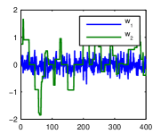
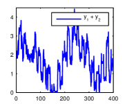
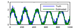
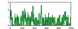
We generate data under this model for $T=50000$ time points and consider increasingly specialized optimization objectives while measuring the error in recovering $Y^{\star}=XD(\theta^{\star})+W$, the underlying source signals corrupted by noise. As can be seen in Table 1, by using $\ell_{1}$ loss for $y_{2}$ and adding $g_{i}(y_{i})$ terms penalizing $\|Dy_{1}\|_{2}^{2}$ and $\|Dy_{2}\|_{1}$, error decreases by 25% over just $\ell_{2}$ loss alone; in Figure 2, we observe that our estimations recovers the true source signals closely with the $g_{i}$ terms helping to capture the dynamics of the noise model for $w_{2}$.

As a baseline for this result, we compare to an unsupervised method, nonnegative sparse coding [10]. We apply sparse coding by segmenting the input signal into $1000$ examples of $50$ time points (1/4 the period of the sine wave, $X_{1}(t)$) and fit a sparse model of 200 basis functions. We report the best possible source separation by assigning each basis function according to an oracle measuring correlation with the true source signal and using the best value over a grid of hyperparameters; however, performance is still significantly worse than the contextually supervised method which makes explicit use of additional information.

Table 1: Comparison of models for source separation on synthetic data.

Model	RMSE
Nonnegative sparse coding	0.4035
$\ell_{2}$ loss for $y_{1}$	0.1640
$\ell_{2}$ loss for $y_{1}$, $\ell_{1}$ loss for $y_{2}$	0.1520
$\ell_{2}$ loss for $y_{1}$, $\ell_{1}$ loss for $y_{2}$ and $g_{i}$ penalizing $\|Dy_{i}\|$	0.1217

Energy disaggregation on smart meter data. Next, we turn to the motivating problem for our model: disaggregating large-scale low resolution smart meter data into its component sources of consumption. Our dataset comes from PG&E and was collected by the utility from customers in Northern California who had smart meters between 1/2/2008 and 12/31/2011. According to estimations based on survey data, heating and cooling (air conditioning and refrigerators) comprise over 39% of total consumer electricity usage [1] and thus are dominant uses for consumers. Clearly, we expect temperature to have a strong correlation with these uses and thus we provide contextual supervision in the form of temperature information. The PG&E data is anonymized, but the location of individual customers is identified at the census block level; we use this information to construct a parallel temperature dataset using data from Weather Underground (http://www.wunderground.com/).

The exact specification of our energy disaggregation model is given in Table 2—we capture the non-linear dependence on temperature with radial-basis functions (RBFs), include a “Base” category which models energy used as a function of time of day, and featureless “Other” category representing end-uses not explicitly modeled. For simplicity, we penalize each category’s deviations from the model using $\ell_{1}$ loss; but for heating and cooling we first multiply by a smoothing matrix $S_{n}$ ($1$’s on the diagonal and $n$ super diagonals) capturing the thermal mass inherent in heating and cooling: we expect energy usage to correlate with temperature over a window of time, not immediately. Finally, we use $g_{i}(y_{i})$ and the difference operator to encode our intuition of how energy consumption in each category evolves over time. The “Base” category represents an aggregation of many sources of consumption and which we expect to evolve smoothly over time, while the on/off behavior in other categories is best represented by the $\ell_{1}$ penalty.

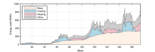
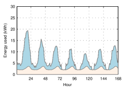
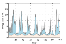
We present the result of our model at two time scales, starting with Figure 3 (top), where we show aggregate energy consumption across all homes at the week level to demonstrate basic trends in usage. Quantitatively, our model assigns 15.6% of energy consumption to “Cooling” and 7.7% to “Heating”, which is reasonably close to estimations based on survey data [1] (10.4% for air conditioning and 5.4% for space heating). We have deliberately kept the model simple and thus our higher estimations are likely due to conflating other temperature-related energy usages, such as refrigerators and water heating. In Figure 3 (bottom), we present the results of the model in disaggregating energy usage for a single hot summer week where the majority of energy usage is estimated to be cooling due to the context provided by high temperature.

Table 2: Model specification for contextually supervised energy disaggregation.

Category	Features	$\ell_{i}$	$g_{i}$
Base	Hour of day	$\|y_{1}-X_{1}\theta_{1}\|_{1}$	$\|Dy_{1}\|_{2}^{2}$
Cooling	RBFs over temperatures $>70^{\circ}\mathrm{F}$	$\|S_{2}(y_{2}-X_{2}\theta_{2})\|_{1}$	$0.1\times\|Dy_{2}\|_{1}$
Heating	RBFs over temperatures $<50^{\circ}\mathrm{F}$	$\|S_{2}(y_{3}-X_{3}\theta_{3})\|_{1}$	$0.1\times\|Dy_{3}\|_{1}$
Other	None	$\|y_{4}\|_{1}$	$0.05\times\|Dy_{4}\|_{1}$

Figure 3: Disaggregated energy usage for 1276 homes over nearly four years shown weekly (top); and for a single home near Fresno, California over the week starting 6/28/2010 (bottom) with estimated correlations $X_{i}\hat{\theta}_{i}$ (left) and estimated energy uses $\hat{y}_{i}$ (right).

6 Conclusion and discussion

We believe the advances in this work, formalizing contextually supervised source separation and theoretically analyzing the requirements for accurate source signal recovery, will enable new applications of single-channel source separation in domains with large amounts of data but no access to explicit supervision. In energy disaggregation, this approach has allowed us to reasonably separate sources of consumption from extremely low-frequency smart meter data. This a significant advancement with the potential to drive increases in energy efficiency through programs that expose this information to consumers and automated systems for demand response. Developing algorithms that use this information to achieve these goals is an interesting direction for future work.

Another interesting direction is the explicit connection of our large-scale low-resolution methods with the more sophisticated appliance models developed on smaller supervised datasets with high-frequency measurements. As a few examples, a small amount of supervised information would enable us to calibrate our models automatically, while a semi-supervised approach would enable spreading some of the benefit of high-resolution load monitoring to the vast number of homes where only smart meter data is available.

References

- [1] 2009 RECS survey data. Available at http://www.eia.gov/consumption/residential/data/2009/.
- [2] A. J. Bell and T. J. Sejnowski. An information-maximization approach to blind separation and blind deconvolution. Neural computation, 7(6):1129–1159, 1995.
- [3] T. Blumensath and M. Davies. Shift-invariant sparse coding for single channel blind source separation. SPARS, 5:75–78, 2005.
- [4] P. Comon. Independent component analysis, a new concept? Signal processing, 36(3):287–314, 1994.
- [5] S. Darby. The effectiveness of feedback on energy consumption. Technical report, Environmental Change Institute, University of Oxford, 2006.
- [6] M. Davies and C. James. Source separation using single channel ica. Signal Processing, 87(8):1819–1832, 2007.
- [7] K. Ehrhardt-Martinez, K. A. Donnelly, and S. Laitner. Advanced metering initiatives and residential feedback programs: a meta-review for household electricity-saving opportunities. In American Council for an Energy-Efficient Economy, 2010.
- [8] Z. Ghahramani and M. I. Jordan. Factorial hidden markov models. Machine learning, 29(2-3):245–273, 1997.
- [9] G. W. Hart. Nonintrusive appliance load monitoring. Proceedings of the IEEE, 80(12):1870–1891, 1992.
- [10] P. O. Hoyer. Non-negative sparse coding. In Neural Networks for Signal Processing, 2002. Proceedings of the 2002 12th IEEE Workshop on, pages 557–565. IEEE, 2002.
- [11] J. Z. Kolter, S. Batra, and A. Y. Ng. Energy disaggregation via discriminative sparse coding. In Neural Information Processing Systems, pages 1153–1161, 2010.
- [12] J. Z. Kolter and T. Jaakkola. Approximate inference in additive factorial hmms with application to energy disaggregation. In International Conference on Artificial Intelligence and Statistics, pages 1472–1482, 2012.
- [13] M. S. Lewicki and T. J. Sejnowski. Learning overcomplete representations. Neural computation, 12(2):337–365, 2000.
- [14] B. Neenan and J. Robinson. Residential electricity use feedback: A research synthesis and economic framework. Technical report, Electric Power Research Institute, 2009.
- [15] B. A. Olshausen, D. J. Field, et al. Sparse coding with an overcomplete basis set: A strategy employed by vi? Vision research, 37(23):3311–3326, 1997.
- [16] O. Parson, S. Ghosh, M. Weal, and A. Rogers. Non-intrusive load monitoring using prior models of general appliance types. In 26th AAAI Conference on Artificial Intelligence, 2012.
- [17] S. T. Roweis. One microphone source separation. Advances in neural information processing systems, pages 793–799, 2001.
- [18] M. Schmidt and R. Olsson. Single-channel speech separation using sparse non-negative matrix factorization. 2006.
- [19] M. N. Schmidt and M. Mørup. Nonnegative matrix factor 2-d deconvolution for blind single channel source separation. In Independent Component Analysis and Blind Signal Separation, pages 700–707. Springer, 2006.
- [20] P. Smaragdis, B. Raj, and M. Shashanka. A probabilistic latent variable model for acoustic modeling. Advances in models for acoustic processing, NIPS, 148, 2006.
- [21] Various. Utility-scale smart meter deployments, plans, and proposals. Technical report, Institute for Electric Efficiency, 2012.
- [22] M. Ziefman and K. Roth. Nonintrusive appliance load monitoring: Review and outlook. IEEE Transactions on Consumer Electronics, 57(1):76–84, 2011.