Update on the 2+1+1 flavor QCD equation of state with HISQ

Abstract:

We present recent results on the QCD equation of state with 2+1+1 flavors of highly improved staggered quarks (HISQ). We focus on three sets of ensembles with temporal extent $N_{\tau}=6$, $8$ and $10$, that reach up to temperatures of $967$, $725$ and $580$ MeV, respectively. The strange and charm quark masses are tuned to the physical values and the light quarks mass is set to one fifth of the strange. This corresponds to a Goldstone pion of about $300$ MeV.

1 Introduction

Properties of the high-temperature phase of QCD, the quark-gluon plasma, are currently a subject of investigation in ultra-relativistic heavy-ion collision experiments at RHIC (BNL), LHC (CERN) and planned future experiments FAIR (GSI) and NICA (JINR). The QCD equation of state with 2+1 flavors of quarks has been and is being extensively studied on the lattice [1, 2] and some preliminary results for the 2+1+1 flavor equation of state (i.e. with a dynamical charm quark) are also available [3, 4]. Here we report on the continuation of the study initiated in Ref. [4].

In heavy-ion experiments heavy quarks are absent in the colliding nuclei and are created at early stages of the collision. Therefore they play an important role, both theoretically and experimentally, as probes of the deconfined medium. Although the charm quark mass is on the order of 10$T_{c}$ ($T_{c}=154(9)$ MeV being the chiral crossover temperature [5]), perturbative [6] and quenched charm lattice [7] calculations indicate that the charm contribution to the equation of state becomes non-negligible at temperatures as low as 2-3$T_{c}$. These temperatures are within reach of the heavy-ion program at LHC. Therefore, it seems timely to include the dynamical charm quark in ab initio QCD calculations.

2 Lattice setup

Calculation of the equation of state on the lattice is computationally expensive because it requires subtraction of ultra-violet divergences, and both finite- and zero-temperature ensembles with large statistics are needed at every value of the gauge coupling. Therefore this study has been done along the line of constant physics (LCP) with the light quark mass set to $m_{l}=m_{s}/5$ and makes use of a set of the existing MILC zero-temperature ensembles [8] on this LCP.

We use the tadpole one-loop improved gauge action and the highly improved staggered quark (HISQ) action [9]. The HISQ action suppresses the taste-exchange interactions present in the staggered formalism and significantly reduces the mass splittings between various pion tastes. This feature improves the approach to the continuum limit at low temperatures. It is also $O(a^{2})$-improved, with the Naik (three-link) term, which controls scaling at high temperatures. In lattice units the charm quark mass $am_{c}\sim O(1)$, therefore the Naik term includes a mass-dependent correction, $\epsilon_{N}$ [9]. It is derived perturbatively to reproduce the correct charm quark dispersion relation up to $O((am_{c})^{4})$. To set the lattice spacing $a$ we use the scale $r_{1}\simeq 0.31$ fm [10]. The strange and charm quark masses are tuned to the physical values by using the $\pi$, $K$, $\eta_{c}$ and $J/\psi$ masses. The tadpole factor defined from the trace of the plaquette $u_{0}=\left\langle{\rm Tr}U_{p}/3\right\rangle^{1/4}$ is determined during the equilibration of the zero-temperature ensembles. We used finite-temperature lattices with aspect ratio of four and temporal extent $N_{\tau}=6$, $8$ and $10$. (In this round we did not pursue the exploratory $N_{\tau}=12$ ensembles reported in Ref. [4], since to get a reliable signal would require significant computational resources.) The temperature is set as $T=1/(aN_{\tau})$.

We determined the $\beta$-functions by fitting the data to the following Ansätze. For the lattice spacing:

$$\frac{r_{1}}{a}(\beta)=\frac{c_{r}^{(0)}f(\beta)+c_{r}^{(2)}(10/\beta)f^{3}(\beta)}{1+d_{r}^{(2)}(10/\beta)f^{2}(\beta)}\,,$$ (1)

and for the strange and charm quark masses:

$$am_{q}(\beta)=\frac{c_{q}^{(0)}f(\beta)+c_{q}^{(2)}(10/\beta)f^{3}(\beta)}{1+d_{q}^{(2)}(10/\beta)f^{2}(\beta)}\,\left(\frac{20b_{0}}{\beta}\right)^{4/9}$$ (2)

where $q=s,c$ and

$$f(\beta)=\left(\frac{10b_{0}}{\beta}\right)^{-b_{1}/(2b^{2}_{0})}\exp{(-\beta/20b_{0})}$$ (3)

is the perturbative two-loop $\beta$-function for three flavors. We checked that using the four-flavor $\beta$-function renormalizes the coefficients but produces the same (within the numerical accuracy) results for the scale and quark masses.

The parameters and accumulated statistics for the zero-temperature ensembles are shown in Table 1. The entries marked with asterisk are used to set the LCP and lattice scale. Corresponding temperatures and the statistics for the finite-temperature ensembles are shown in Table 2.

$\beta$	$am_{s}$	$am_{c}$	$u_{0}$	$\epsilon_{N}$	$a$, fm	size	TU/$10^{3}$
5.400*	0.091	1.339	0.83496	-0.7995	0.220	$16^{3}\times 40$	5.0
5.469	0.0928	1.263	0.838768	-0.6905	0.206	$24^{3}\times 32$	9.7
5.541	0.0859	1.157	0.842646	-0.5797	0.192	$24^{3}\times 32$	9.7
5.600*	0.0785	1.080	0.845768	-0.5168	0.181	$16^{3}\times 48$	12.5
5.663	0.0753	0.996	0.848919	-0.4571	0.170	$24^{3}\times 32$	9.7
5.732	0.0697	0.913	0.852242	-0.4024	0.159	$32^{4}$	3.8
5.800*	0.065	0.838	0.85535	-0.3582	0.151	$16^{3}\times 48$	98.8
5.855	0.0608	0.782	0.857786	-0.3195	0.140	$32^{4}$	12.1
5.925	0.0561	0.716	0.860718	-0.2784	0.130	$32^{4}$	14.5
6.000*	0.0509	0.635	0.86372	-0.2308	0.121	$24^{3}\times 64$	11.4
6.060	0.0481	0.603	0.865978	-0.2010	0.113	$32^{4}$	9.7
6.122	0.0448	0.558	0.86824	-0.1838	0.106	$32^{4}$	9.7
6.180	0.042	0.518	0.870236	-0.1613	0.100	$32^{4}$	7.8
6.238	0.0392	0.482	0.872177	-0.1418	0.094	$32^{4}$	9.7
6.300*	0.037	0.440	0.874164	-0.1204	0.089	$32^{3}\times 96$	6.0
6.530	0.028	0.338	0.880888	-0.0734	0.070	$36^{3}\times 48$	2.8
6.720*	0.024	0.286	0.885773	-0.0533	0.058	$48^{3}\times 144$	5.9
7.000*	0.0158	0.188	0.892186	-0.0235	0.045	$64^{3}\times 192$	0.7
7.140	0.0145	0.172	0.895074	-0.0197	0.039	$64^{3}\times 72$	1.3
7.285	0.0124	0.148	0.89789	-0.0146	0.034	$64^{3}\times 96$	0.9

Table 1: The parameters of the HISQ ensembles along the $m_{l}=m_{s}/5$ LCP: inverse gauge coupling $\beta=10/g^{2}$, input strange and charm quark masses, tadpole factor $u_{0}$, the Naik term correction $\epsilon_{N}$, approximate lattice spacing $a$, lattice volume and the statistics in thousands of molecular dynamics time units.

	$N_{\tau}=6$		$N_{\tau}=8$		$N_{\tau}=10$
$\beta$	$T$	TU/$10^{3}$	$T$	TU/$10^{3}$	$T$	TU/$10^{3}$
5.400	149	10
5.469	160	34
5.541	171	34
5.600	182	10	136	20
5.663	193	34	145	30
5.732	207	30	155	42
5.800	218	10	163	10	131	40
5.855	235	30	176	45	140	42
5.925	253	30	190	45	152	42
6.000	272	10	204	10	163	40
6.060	291	30	218	39	175	42
6.122	310	30	233	39	186	42
6.180			247	11	197	40
6.238					210	14
6.300	369	10	277	10	222	10
6.530			352	11	282	9
6.720	567	10	425	10	340	10
7.000			548	8	438	20
7.140	843	7	632	11	506	19
7.285	967	3	725	11	580	17

Table 2: Inverse gauge coupling, temperatures and the statistics in thousands of molecular dynamics time units for the HISQ finite-temperature ensembles along the $m_{l}=m_{s}/5$ LCP.

3 Trace anomaly

At lattice spacing $a$ the trace of the energy-momentum tensor, or interaction measure, can be related to the partition function as

$$\varepsilon-3p=-\frac{T}{V}\frac{d\ln Z}{d\ln a},\,\,\,\,\,\,\,\,\,\,\,\,\,Z=\int DUD\bar{\psi}D\psi\exp\left(-S_{g}-S_{f}\right),$$ (4)

where $\varepsilon$ is the energy density and $p$ is the pressure.

To normalize the trace anomaly to zero at zero temperature one can take a difference between the finite- and zero-temperature observables at the same values of the gauge coupling and quark masses, i.e. for an observable $X$:

$$\Delta(X)=\langle X\rangle_{\tau}-\langle X\rangle_{0}\,.$$ (5)

The trace anomaly is then given in terms of the basic observables that enter into the action:

$$\frac{\varepsilon-3p}{T^{4}} = -R_{\beta}(\beta)\left[\Delta(S_{g})+R_{u}(\beta)\Delta\left(\frac{dS_{g}}{du_{0}}\right)\right]+R_{\beta}(\beta)R_{m_{s}}(\beta)\left[2m_{l}\Delta(\bar{\psi}_{l}\psi_{l})+m_{s}\Delta(\bar{\psi}_{s}\psi_{s})\right]$$ (6)

$$+ R_{\beta}(\beta)R_{m_{c}}(\beta)\left[m_{c}\Delta(\bar{\psi}_{c}\psi_{c})+R_{\varepsilon_{N}}(\beta)\Delta\left(\bar{\psi}_{c}\left[\frac{dM_{c}}{d\varepsilon_{N}}\right]\psi_{c}\right)\right]\,.$$

The change of the lattice spacing and the parameters of the action along the LCP are controlled by the $\beta$-functions:

$$R_{\beta}(\beta) = T\frac{{\rm d}\beta}{{\rm d}T}=-a\frac{{\rm d}\beta}{{\rm d}a}=(r_{1}/a)(\beta)\,\left(\frac{{\rm d}(r_{1}/a)(\beta)}{{\rm d}\beta}\right)^{-1}\,,$$ (7)

$$R_{m_{q}}(\beta) = \frac{1}{am_{q}(\beta)}\frac{{\rm d}am_{q}(\beta)}{{\rm d}\beta}\qquad\text{for}~{}q=s,c\,,$$ (8)

$$R_{u}(\beta) = \beta\frac{{\rm d}u_{0}(\beta)}{{\rm d}\beta}\,,$$ (9)

$$R_{\epsilon}(\beta) = \frac{{\rm d}\epsilon_{N}(\beta)}{{\rm d}\beta}\,.$$ (10)

As function of $\beta$ the tadpole factor $u_{0}$ is fit to $u_{0}(\beta)=c_{1}+c_{2}e^{-d_{1}\beta}$, and the Naik term correction $\epsilon_{N}$ to a polynomial in $\beta$.

Figure 1: Contributions to the trace anomaly from the gauge field (top left), valence light (top right), strange (bottom left) and charm (bottom right) quarks.

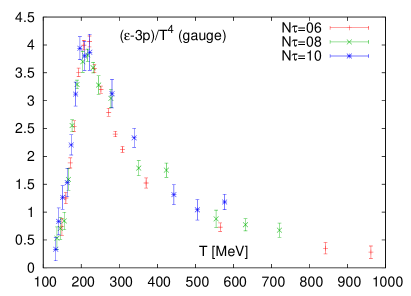
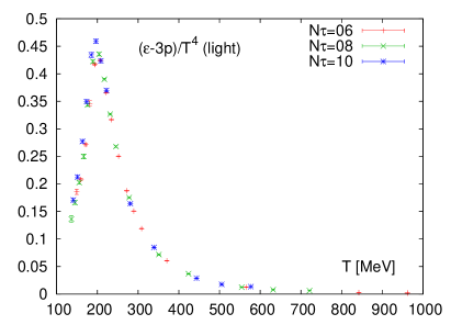
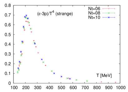
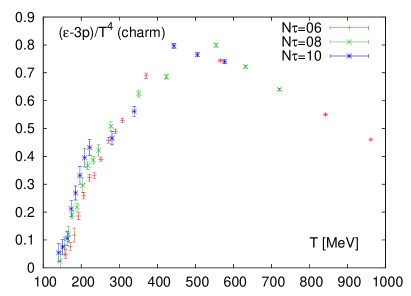
The first term in Eq. (6) describes the contribution to the trace anomaly from the gauge field, the second from the (valence) light and strange quarks and the third from the (valence) charm quark. These four quantities are shown in Fig. 1. In the peak region around 200 MeV the trace anomaly is dominated by the gauge part. Light and strange quark contributions also reach their maxima around that temperature, while the charm part at 200 MeV contributes less than 10% to the total result. The charm contribution reaches its maximum around 500 MeV and accounts for 40% of the value of the trace anomaly at that temperature. (Note, that this is the dominant, valence, charm quark contribution, while the effect of the sea charm can only be quantified by comparing to the 2+1 flavor equation of state. Such an analysis is left for the future.)

Figure 2: The trace anomaly at low temperatures (left) and in the peak region (right). Bands represent statistical errors on the spline fits.

The contribution due to the variation of the charm quark mass in the Naik term, $dM_{c}/d\epsilon_{N}$ is larger on coarser lattices. We have evaluated it on $N_{\tau}=6$ lattices at $T=272$ and $369$ MeV, and corresponding zero-temperature ensembles. This quantity is about 2% of the total result, which is comparable to the statistical errors. Therefore in the present analysis, in particular, for the quantity in Fig. 1 (bottom right) and for the total trace anomaly, we did not include the term $\Delta(\bar{\psi}_{c}[dM_{c}/d\varepsilon_{N}]\psi_{c})$. Its inclusion will presumably decrease the cutoff effects on the charm contribution at low temperatures, $150-200$ MeV.

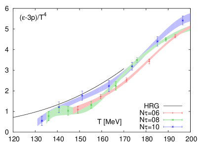
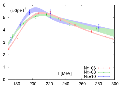
We fitted the data for the trace anomaly with splines, shown as bands in Fig. 2. The width of the bands represents only the statistical error, estimated by bootstrap. In Fig. 2 (left) the low-temperature region is shown. The solid line is the hadron resonance gas (HRG) model result. Coarser lattices produce a heavier hadron spectrum, thus, the approach to the continuum is from below (at least, when the temperature is set with the $r_{1}$ scale). In the peak region, Fig. 2 (right), the cutoff effects are mild, and at temperatures around 200 MeV and above, where the light hadrons melt, they are presumably not caused by taste symmetry breaking in the quark sector.

Figure 3: The 2+1+1 flavor trace anomaly with HISQ along the $m_{l}=m_{s}/5$ LCP.

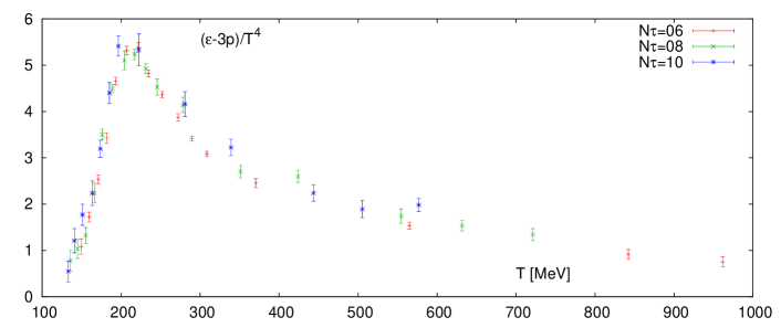
The total trace anomaly is shown in Fig. 3. The $N_{\tau}=10$ lattices extend to 580 MeV. This is enough to cover the peak of the valence charm contribution, but without further $N_{\tau}=10$ data the cutoff effects above this temperature are thus hard to quantify.

4 Conclusion

We have extended our calculation of the 2+1+1 flavor QCD equation of state with highly improved staggered quarks in two ways. We generated several new zero- and finite-temperature ensembles to provide better coverage of temperatures in the range 130-1000 MeV and substantially increased the statistics on most of the finite temperature ensembles. We have reached lattice spacings down to $0.034$ fm, which corresponds to 967 MeV on the coarsest, $N_{\tau}=6$ lattice. The charm contribution to the trace anomaly becomes non-negligible around 300 MeV and reaches the maximum far in the deconfined phase, around 500 MeV. The cutoff effects on the trace anomaly are significant at low temperatures and are mild in the peak region. However, $N_{\tau}=12$ ensembles will be needed for a reliable continuum extrapolation.

References

- [1] A. Bazavov et al. [HotQCD], Phys. Rev. D 80, 014504 (2009) [arXiv:0903.4379 [hep-lat]]; A. Bazavov [HotQCD], Nucl. Phys. A904-905 2013, 877c (2013) [arXiv:1210.6312 [hep-lat]].
- [2] Y. Aoki, Z. Fodor, S. D. Katz and K. K. Szabo [Budapest-Wuppertal], JHEP 0601, 089 (2006) [hep-lat/0510084]; S. Borsanyi et al. [Budapest-Wuppertal], JHEP 1011, 077 (2010) [arXiv:1007.2580 [hep-lat]]; S. Borsanyi et al. [Budapest-Wuppertal], arXiv:1309.5258 [hep-lat].
- [3] S. Borsanyi et al. [Budapest-Wuppertal], PoS LATTICE 2011, 201 (2011) [arXiv:1204.0995 [hep-lat]]; C. Ratti et al. [Budapest-Wuppertal], Nucl. Phys. A 904-905, 869c (2013).
- [4] A. Bazavov et al. [MILC], PoS LATTICE 2012, 071 (2012).
- [5] A. Bazavov et al. [HotQCD], Phys. Rev. D 85, 054503 (2012) [arXiv:1111.1710 [hep-lat]].
- [6] M. Laine and Y. Schroder, Phys. Rev. D 73, 085009 (2006) [hep-ph/0603048].
- [7] M. Cheng [RBC-Bielefeld], PoS LAT 2007, 173 (2007) [arXiv:0710.4357 [hep-lat]]; L. Levkova, PoS LAT 2009, 170 (2009) [arXiv:0910.3006 [hep-lat]]; C. DeTar et al. [MILC], Phys. Rev. D 81, 114504 (2010) [arXiv:1003.5682 [hep-lat]].
- [8] A. Bazavov et al. [MILC], Phys. Rev. D 82, 074501 (2010) [arXiv:1004.0342 [hep-lat]]; A. Bazavov et al. [MILC], Phys. Rev. D 87, 054505 (2013) [arXiv:1212.4768 [hep-lat]].
- [9] E. Follana et al. [HPQCD/UKQCD], Phys. Rev. D 75, 054502 (2007) [hep-lat/0610092].
- [10] R. Sommer, Nucl. Phys. B 411, 839 (1994) [hep-lat/9310022]; C. W. Bernard et al. [MILC], Phys. Rev. D 62, 034503 (2000) [hep-lat/0002028].