Complete QED NLO contributions to the reaction $e^{+}e^{-}\to\mu^{+}\mu^{-}\gamma$ and their implementation in the event generator PHOKHARA

Abstract

KLOE and Babar have an observed discrepancy of 2% to 5% in the invariant pion pair production cross section. These measurements are based on approximate NLO $\mu^{+}\mu^{-}\gamma$ cross section predictions of the Monte Carlo event generator PHOKHARA7.0. In this article, the complete NLO radiative corrections to $\mu^{+}\mu^{-}\gamma$ production are calculated and implemented in the Monte Carlo event generator PHOKHARA9.0. Numerical reliability is guaranteed by two independent approaches to the real and the virtual corrections. The novel features include the contribution of pentagon diagrams in the virtual corrections, which form a gauge-invariant set when combined with their box diagram partners. They may contribute to certain distributions at the percent level. Also the real emission was complemented with two-photon final state emission contributions not included in the generator PHOKHARA7.0. We demonstrate that the numerical influence reaches, for realistic charge-averaged experimental setups, not more than 0.1% at KLOE and 0.3% at BaBar energies. As a result, we exclude the approximations in earlier versions of PHOKHARA as origin of the observed experimental discrepancy.

1 Introduction

The total cross section for electron-positron annihilation into hadrons is a very important physical observable weighting significantly on the theory error of the muon anomalous magnetic moment and the running electromagnetic fine structure constant used in the tests of the Standard Model and its extensions. For recent reviews see e.g. Actis:2010gg ; Hagiwara:2011af ; Davier:2010nc ; Jegerlehner:2009ry ; Harlander:2002ur . At high energies, the cross section can be calculated using perturbative QCD, however at low energies one has to rely on the experimental measurements.

One of the methods used to extract the hadronic cross section is the ”radiative return”, exploiting the fact that the cross section of the process with initial state photon radiation can be factorised into a known perturbative factor and the hadronic cross section without initial state radiation at the energy lowered by the emitted photons. Due to the complexity of the experimental setup, the extraction of the hadronic cross section within a realistic experimental framework can be achieved only by means of an event generator.

The most important contribution to the hadronic cross section is the pion pair production channel. Its accuracy is an issue as it provides the main source of error in the evaluation of the muon anomalous magnetic moment Hagiwara:2011af . In view of the planned improvement of the direct measurement of the muon anomalous magnetic moment Venanzoni:2012vha , with the expected error four times smaller than the present one, it is crucial to pull down the theoretical error as much as possible. The pion production cross section in $e^{+}e^{-}$ scattering was measured, using the radiative return method, by BaBar Lees:2012cj ; Aubert:2009ad and KLOE Babusci:2012rp ; Ambrosino:2010bv ; Ambrosino:2008aa . Both experiments quote individual errors at the level of a fraction of a percent, while the discrepancy between them is up to 2% at the $\rho$ peak and 5% when approaching the energy of 1 GeV. The origin of the discrepancy remains unclear. Since both experiments use the PHOKHARA Czyz:2002np ; Czyz:2005as event generator to extract the hadronic cross section, it is necessary to check carefully its physical content. The PHOKHARA event generator was used to generate the reactions $e^{+}e^{-}\to\pi^{+}\pi^{-}+\ {\rm photons}$ and $e^{+}e^{-}\to\mu^{+}\mu^{-}+\ {\rm photons}$. The latter process is used for monitoring the luminosity. So far, the version of PHOKHARA used by BaBar and KLOE included the dominant next-to-leading order (NLO) radiative corrections. In view of the above mentioned discrepancy between BaBar and KLOE, it is essential to make a full NLO calculation and to establish the importance of the missing contributions.

In this article, the complete radiative NLO Quantum Electrodynamics (QED) corrections to the reaction $e^{+}e^{-}\to\mu^{+}\mu^{-}\gamma$ are calculated, tested and implemented into the event generator PHOKHARA. From a technical point of view, the pentagon diagrams are the most challenging. Because there is no scale available which might lead to logarithmically enhanced contributions, they are expected to be small. However, it is known that logarithmic enhancements can be generated in some regions of the phase space within complicated experimental setups. The fact that we can not neglect the small electron mass for the same reason poses an additional challenge in the calculation of the virtual amplitudes since ratios of the order of $s/m_{e}^{2}$ can appear, where $s$ is the energy of the collider. This demands a good control on the numerical accuracy of our amplitudes . Consequently, detailed Monte Carlo studies are mandatory. First studies were presented some time ago by the Katowice/Zeuthen group Kajda:2009aa , in PhD theses kajphd ; yundin-phd-2012–oai:export and also by an independent alternative approach Actis:2009zz ; Actis:2009uq . This enabled us to compare specific phase space points with Actis:2009zz ; Actis:2009uq with high precision as a first numerical test; see Ref. yundin-phd-2012–oai:export for details. Here, we perform a complete calculation in the frame of a realistic Monte Carlo environment, PHOKHARA9.0. Because there are several known sources of numerical instabilities, and because we have no external cross-check available, we organized for two independent implementations of the QED virtual corrections. Having implemented the complete radiative corrections, detailed physics studies became possible, and their results are presented here.

The article is organised as follows: In Section 2 and Appendices B and C we give a detailed description of the calculation of the radiative corrections. Section 3 sketches the implementation of the radiative corrections into PHOKHARA9.0. In Section 4, the main tests of the correctness and the numerical stability of the code are presented. Further, the relevance of the NLO radiative corrections, which were missing in PHOKHARA7.0, is investigated. In Section 5, the possible impact of the radiative corrections, analogous to those studied here, on the pion form factor measurements of BaBar and KLOE is discussed. Section 6 contains the conclusions.

2 Radiative corrections to $e^{+}e^{-}\to\mu^{+}\mu^{-}\gamma$

The tree level diagrams contributing to the leading order (LO) amplitude are shown in Fig. 2.1. There are two types of contributions, those with initial state photon emission (ISR) and final state photon emission (FSR). The ISR and FSR pairs of diagrams are separately gauge invariant.

Figure 2.1: The tree diagrams for $e^{+}e^{-}\to\mu^{+}\mu^{-}\gamma$.

At NLO QED, there are the virtual and the real corrections resulting in three types of contributions to the cross section, the ISR and the FSR contributions, and their ISR-FSR interference terms.

We use dimensional regularization 'tHooft:1972fi to regularize the ultraviolet (UV) and infrared (IR) divergences. The UV divergences of the virtual amplitude are removed by the renormalization counter-terms. Both the virtual and the real corrections are infrared divergent. These divergences cancel in the sum for infrared-safe observables. The IR divergences are canceled and both the virtual+real (soft) and the real (hard) corrections become separately numerically integrable. Details of the real emission calculation are given in Section 2.2. In the following, we describe the method used to compute the virtual amplitudes.

2.1 Virtual corrections

Besides photonic self-energy corrections, there are 32 diagrams contributing to $e^{+}e^{-}\to\mu^{+}\mu^{-}\gamma$ at NLO QED. They can be classified into several independent gauge invariant subsets, which we will call Penta-Box, Box-Triangle-Bubble and Triangle contributions. The first class involves loop corrections with the two lepton lines attached to the loop. The most challenging diagrams are the four pentagon diagrams, shown in Fig. 2.2, where a real photon is emitted from an internal line.

Figure 2.2: The four diagrams with pentagon topology for $e^{+}e^{-}\to\mu^{+}\mu^{-}\gamma$

They do not constitute a class of gauge independent diagrams by themselves. Gauge invariant groups are formed when a pentagon is associated with two box diagrams where a photon is radiated from the same external (electron or muon) line. This is shown schematically in Fig. 2.3. The contribution of these twelve Penta-Box diagram combinations, interfering with the tree level diagrams of Fig. 2.1, will be discussed in detail in Section 4.

Figure 2.3: One of the four gauge invariant combinations of a pentagon with two boxes with external photon emission for $e^{+}e^{-}\to\mu^{+}\mu^{-}\gamma$.

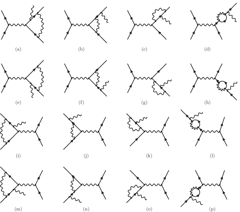
Box-Triangle-Bubble and Triangle contributions contain corrections to one lepton line (electron or muon) and are further classified depending whether the loop and the real photon are attached to the same lepton line. The Box-Triangle-Bubble class contains all the loop corrections to a lepton line with a real (on-shell) photon and a second off-shell photon, connecting to the other lepton line. The contributing boxes, vertices and bubbles can be found in Fig. 2.4. There are two independent gauge invariant subsets, for FSR (two upper lines of Fig. 2.4) and for ISR (two lower lines of Fig. 2.4). The triangle contributions are given in Fig. 2.5. There, a real photon is emitted from one fermion line, and the other photon (off-shell) entering a 3-point function is connected to the other fermion line.

Figure 2.4: The set of sixteen one-loop Box, triangle and self-energy diagrams with internal photon emission in $e^{+}e^{-}\to\mu^{+}\mu^{-}\gamma$.

Figure 2.5: The four triangle diagrams with external photon emission in $e^{+}e^{-}\to\mu^{+}\mu^{-}\gamma$.

Finally, we mention the diagrams with external photon emission and self-energy insertions to the photon propagator . They constitute a gauge-invariant universal correction which can be accounted for in any QED calculation by simply running the fine structure constant to the appropriate scale Bohm:1986rj ; Denner:1991kt . These self-energies are treated separately and have been omitted from our fixed-order loop amplitude definition in Fig. 2.4. The treatment of vacuum polarisation in the PHOKHARA event generator, together with narrow resonance contributions is described in detail in Ref. Czyz:2010hj and will not be discussed here.

In the present article, two independent programs using two different methods are used. One is based on the trace method and the calculations are done using double precision numerical routines, including the PJFry libraries pjfry-project . We refer to it as “Double precision - Trace method” (DT-method). The other one is based on the helicity formalism as described in Ref. Campanario:2011cs , and we refer to it as “Quadruple precision - Helicity method” (QH-method) because numerical calculations are done partially using quadruple precision. Such independent implementations are necessary to gain sufficient numerical reliability.

2.1.1 The DT-method

With the DT-method, topologies are generated by QGRAF Nogueira:1991ex and then dressed with particles and momenta by the DIANA program Tentyukov:1999is according to the QED model description file. The resulting output contains a list of Feynman diagrams in the textual representation, which is defined by the TML markup language script Tentyukov:1999yq . Next, the diagrams are passed through the FORM Vermaseren:2000nd script, which substitutes Feynman rules according to the selected model. Further manipulations are done with FORM. In addition, some general simplifications can be enabled by setting configuration parameters. This includes gamma algebra identities like $\gamma^{\mu}\gamma^{\nu}\gamma_{\mu}=(2-d)\gamma^{\nu}$, the transversality condition, e.g. $p_{1}\cdot\epsilon(p_{1})=0$, usage of Dirac equation and momentum conservation. The resulting expressions are written in the FORM tablebase. We use it as an input in the squaring program which sums the diagrams and multiplies them by the complex conjugated set of Born diagrams. The fermion lines are connected by the completeness relation. Then, Dirac traces are taken.

For the calculation of the newly added one-loop pentagon contributions, one has to calculate 5-point tensor Feynman integrals up to rank $R=3$. We reduce the tensor integrals in $d=4-2\epsilon$ dimensions to scalar 1- to 4-point functions. They depend on the reduction basis chosen. Often one uses as basis momenta, the external momenta of the diagram as in Refs. Passarino:1978jh ; Campanario:2011cs . Our choice (with a one-to-one correspondence) are the so-called chords, the shifts of internal momenta with respect to the loop momentum pjfry-project .

Advanced tensor integral calculations became a standard task in recent years, mainly triggered by LHC physics. Nevertheless, ensuring sufficient numerical stability is demanding for several reasons. An often discussed issue is the treatment (or avoidance) of small or vanishing inverse Gram determinants. Another one is just the extreme spread of scales met in our physical process, because we cannot neglect the electron mass $m_{e}\approx 1/2000$ GeV as an independent parameter. With $\sqrt{s}=1-10$ GeV, one faces e.g. a ratio $m_{e}^{2}/s\sim 10^{-7}-10^{-9}$. The DT implementation of tensor integral calculation relies on the approach developed in Refs. Davydychev:1991va ; Tarasov:1996br ; Fleischer:1999hq ; Diakonidis:2008ij ; Diakonidis:2009fx ; Fleischer:2010sq ; Almasy:2013uwa and uses the PJFry tensor reduction package yundin-phd-2012–oai:export ; Fleischer:2011zz , combined with QCDLoop/FF Ellis:2007qk ; vanOldenborgh:1990yc or OneLOop vanHameren:2010cp for scalar integrals. More technical details can be found in Ref. yundin-phd-2012–oai:export  .

2.1.2 The QH-method

The second implementation (QH-method) uses the helicity formalism as described in Ref. Campanario:2011cs . To build the virtual amplitude, four building blocks are used. Corrections to a lepton line with two real (on-shell or off-shell) photons attached in a fixed order of external bosons, Fig. 2.6, constitute the first building block, which we call Boxline and also include the corresponding counter-terms which are not shown in Fig. 2.6. We used the effective current approach, thus, $V_{1}$ and $V_{2}$ should be understood as generic off-shell currents which can be, in this case, an on-shell photon or an off-shell photon, which forms the second lepton line. The physical amplitude is built by considering all physical permutations and contractions with external currents yielding the Box-Triangle-Bubble gauge invariant subsets of Fig. 2.4. In addition, we use the vertex corrections to a lepton line with one real photon attached to it. All possible contributions result in the triangle contributions of Fig. 2.5.

Figure 2.6: Boxline contributions for $e^{+}e^{-}\to\mu^{+}\mu^{-}\gamma$.

The third building group is formed by the Penta-Box diagrams depicted in Fig. 2.3, which involve the pentagon diagrams. The last building block is obtained by crossing the two initial fermion lines in Fig. 2.3 and constitute an independent gauge group. To compute them, we generalized the software developed in Ref. Campanario:2011cs to be able to compute diagrams with two fermion lines. This includes the use of Chisholm identities Sirlin:1981pi which reduces the CPU time required to evaluate the Penta-Box contributions by a factor ten. At the same time, this improves the stability of the code since it makes explicit terms proportional to the small electron mass. The calculation of tensor integrals is done by using Passarino-Veltman reduction Passarino:1978jh for up to $4$-point diagrams and the method of Denner:2005nn ; Binoth:2005ff , following the convention of Ref. Campanario:2011cs for higher-point tensor integrals. The scalar integrals are calculated as in Refs. 'tHooft:1978xw ; Denner:1991kt .

We use a cache system in all the building blocks such that the information of the loop-dependent parts are stored. This is particularly important for this process since up to 32 different helicity amplitudes exist corresponding to the different helicity and polarization combinations of the external particles. After the first helicity is computed, which include the evaluation of the loop-dependent parts, any additional helicity amplitude is computed with less than 10$\%$ of CPU time, reducing the CPU time of the code by a factor 10.

The building blocks do not use special properties like transversality or being on-shell for the real photons attached to the lepton lines, instead, we assume external effective current attached to them. This allows us to use Ward identities, by replacing an effective current with the corresponding momentum, to check the accuracy of the computed amplitudes. We classified our contributions in gauge invariant subsets so that the Ward identities are fulfilled. Those identities are called gauge tests and are checked with a small additional computing cost, using the cache system. They are checked for every phase space point and each gauge invariant subset distinguishing between FSR and ISR contributions. This is important because the phase space integration of the virtual contribution shows numerical instabilities in the calculation of the one-loop tensor integrals Campanario:2011cs .

We have implemented a rescue system for phase space points where the Ward identities are not satisfied with an accuracy of at least three digits. First, we calculate the amplitudes applying quadruple precision only to the scalar integrals and tensor reduction routines. This requires reconstructing the external momenta in quadruple precision, so that global energy-momentum conservation is still fulfilled at the higher numerical accuracy retaining the external particles on their mass-shell. If the Ward identities are not satisfied, the rescue system evaluates the amplitude using quadruple precision in all parts of the code. With this system, we find that the proportion of phase space points that do not pass the Ward identities for a requested accuracy of $\epsilon=10^{-3}$ is well below one in ten thousand. The rescue system adds an additional $10\%$ to the CPU time.

Despite the cache system and the use of Chisholm identities, this implementation is still seven times slower that the DT-method which can be traced back to the evaluation of the 32 helicity amplitudes and the parts evaluated in quadruple precision.

We have tried to evaluate the amplitudes only in double precision to improve the speed of the code by a factor two using dedicated subroutines for small Gram determinants. These involve the evaluation of three- and four-point functions up to Rank 11 and 9, respectively, following the notation of Ref. Campanario:2011cs . The high rank of the rescue system allows to obtain full double precision for mild cancellations in the Gram determinants. However, two problems arise. First, for the failing phase space points, there was always some internal combination for which the expansion breaks down due to the presence of additional cancellations in sub-Cayley determinants. Thus, full double precision is not achieved for all tensor integrals coefficients. Second, within the helicity method formalism, there exist extremely large cancellations between the different helicity amplitudes resulting into an additional loss of precision which can be larger than the one due to the presence of small Gram determinants. These numerical cancellations are related to the fact that the mass of the electron has to be retained, and many numerical cancellation occur. For example, in the numerical calculation of $/\kern-6.0pt{p}_{e}u(p_{e})=m_{e}u(p_{e})$ cancellations of the order of $s/m_{e}^{2}$ would appear, where s is the energy of the collider, if the Dirac equation is not applied or is not treated carefully.

These two problems are reflected in a bad accuracy of the gauge test and, therefore, in the large number of identified unstable points using only double precision. The second problem is naturally solved using the DT-method since the summation and averaging over spins are done analytically and many of these numerical cancellations are avoided. We decided to implement the DT-method in PHOKHARA9.0 and compare it with the code implemented in full quadruple precision where the gauge test ensures the numerical accuracy of the code.

2.2 Real photon emission

The real two-photon emission, which contributes to the $e^{+}e^{-}\to\mu^{+}\mu^{-}\gamma$ cross section at NLO is now included in the PHOKHARA code completely in contrast to the implementation of Refs. Rodrigo:2001kf ; Czyz:2004rj , where subleading contributions were neglected. We distinguish between soft and 2-hard photon emission.

2.2.1 Soft photon emission

In the soft photon contribution, the phase space of one of the photons ($k_{1})$ is integrated out analytically. The integrals to be performed, which factorise in front of the square of the full amplitude describing the $e^{+}e^{-}\to\mu^{+}\mu^{-}\gamma$  reaction, read

$$F(p_{1},p_{2},q_{1},q_{2},r)=\frac{-\alpha}{4\pi}\int\frac{d^{3}k_{1}}{E_{k_{1}}}\left[\left(\frac{p_{1}}{p_{1}\cdotp k_{1}}-\frac{p_{2}}{k_{1}\cdotp p_{2}}\right)+\left(\frac{q_{2}}{q_{2}\cdotp k_{1}}-\frac{q_{1}}{k_{1}\cdotp q_{1}}\right)\right]^{2},$$ (2.1)

where $p_{1}$, $p_{2}$, $q_{1}$ and $q_{2}$ are the momenta of the positron, electron, antimuon and muon, respectively. The infrared regulator — the photon mass $\lambda$ and the photon energy cut-off $E_{max}$ dependence can be cast into a single parameter

$$r=\frac{2E_{max}}{\lambda}.$$ (2.2)

In principle, this is a well known formula, which can be found in the literature Berends:1987ab ; Rodrigo:1999qg . However, as the integral over the photon energy is performed only up to a given cut-off $E_{max}$, its form depends on the frame in which this cut-off is applied. We found it suitable to give the formulae, which are valid in any frame in which the cut-off is defined. They are a bit longer than the usual ones as we express everything through the four momenta $p_{1},p_{2},q_{1},q_{2}$ given in the frame, where the cut-off is defined, in contrast to the usual expressions which use invariants, but are less universal. The explicit expression for $F(p_{1},p_{2},q_{1},q_{2},r)$ is given in Appendix C.

2.2.2 Two-hard photon emission

For the two-hard photon emission, the helicity method for the calculation of the amplitudes was used and cross checked with a dedicated code based on the trace method of spin summation. The convention for the helicity amplitude method introduced in Ref. Rodrigo:2001kf was adopted.

The only amplitude, which was missing in earlier versions of PHOKHARA was the two-photon FSR. Interferences between the coded amplitudes, with infrared divergences matching the ones from Penta-Box diagrams, were also not included. After some algebra similar to Refs. Rodrigo:2001kf ; Czyz:2004rj , a very compact form for the two-photon FSR amplitude is obtained

$$\kern-15.0ptM\left(\lambda_{\mu^{+}},\lambda_{\mu^{-}},\lambda_{1},\lambda_{2}\right)=v_{I}^{\dagger}(\lambda_{\mu^{+}})A\left(\lambda_{1},\lambda_{2}\right)u_{I}(\lambda_{\mu^{-}})+v_{II}^{\dagger}(\lambda_{\mu^{+}})B\left(\lambda_{1},\lambda_{2}\right)u_{II}(\lambda_{\mu^{-}})\ ,$$ (2.3)

where the matrices A and B and the convention used to define the spinors are given in Appendix B. The energy of one of the photons has to be bigger than the cut-off $E_{max}$ and the sum of the soft and hard contributions should not depend on this cut-off up to terms $\sim E_{max}$, which are neglected in the analytic calculation.

3 Implementation of the radiative corrections in the event generator PHOKHARA9.0

PHOKHARA9.0 is available from the webpage http://ific.uv.es/~rodrigo/phokhara/. As stated already, all new parts of the released computer code were calculated independently by two methods and/or groups of the authors of this article. To ensure the stability of the virtual corrections, we use the two independent codes described in Section 2. The faster routine in the released version of PHOKHARA9.0 is used, which is the code based on the DT-method. The other one can be obtained on request. We sketch here shortly the new ingredients of the released code. The listed changes concern only the $e^{+}e^{-}\to\mu^{+}\mu^{-}\gamma$ mode, when it is running with the complete NLO radiative corrections:

• The virtual corrections are calculated in double precision and the sum over polarisations is done with the trace method. The software PJFry pjfry-project is used for this purpose and the relevant parts of the libraries developed there are distributed with PHOKHARA9.0.

• The soft photon emission is calculated using the formulae discussed in Section 2.2.1 and in Appendix C.

• The two-hard-photon emission part uses the helicity amplitudes as defined in Ref. Czyz:2004rj . The newly added part — the two photon FSR is described in Section 2.2.2 and coded accordingly.

4 Tests of the code

The released code was tested very extensively both for the real and the virtual contributions to assure the technical accuracy of the code to be much better than the one required for experimental measurements. The necessity of retaining a finite electron mass possesses a potential threat of numerical instabilities both for the real and the virtual contributions since cancellations of the order of $s/m_{e}^{2}$ can appear.

The virtual corrections constitute the most challenging part. The presence of Gram determinants can constitute an additional source of instabilities which can be more challenging for some realistic experimental selection cuts where forward photon emissions are favoured, resulting in collinear photon emissions.

$\sqrt{s}$=1.02 GeV
$\sigma_{QH}$ = 6.332(1) [nb]
$\sigma_{DT}$ = 6.332(1) [nb]
$|\Delta|>$	$\sigma_{\Delta_{DT}}$ [nb]	$\sigma_{\Delta_{QH}}$ [nb]	$\sigma_{\Delta_{DT}}/\sigma_{DT}$	Nevent
0.1	0	0	0	0
0.01	$4(4)\cdotp 10^{-8}$	$4(4)\cdotp 10^{-8}$	$6(6)\cdotp 10^{-9}$	1
0.001	$1.4(3)\cdotp 10^{-6}$	$1.4(3)\cdotp 10^{-6}$	$2.2(4)\cdotp 10^{-7}$	32
0.0001	$2.1(1)\cdotp 10^{-4}$	$2.1(1)\cdotp 10^{-4}$	$3.4(2)\cdotp 10^{-5}$	521
0.00001	$2.7(1)\cdotp 10^{-4}$	$2.7(1)\cdotp 10^{-4}$	$4.2(2)\cdotp 10^{-5}$	787

Table 4.1: Comparison between the codes based on the DT-method and the QH-method at $\sqrt{s}$=1.02 GeV. No selection cuts are applied. See text for details on the definition of the Table entries.

$\sqrt{s}$=10.56 GeV
$\sigma_{QH}$ = 0.07004(4) [nb]
$\sigma_{DT}$ = 0.07004(4) [nb]
$|\Delta|>$	$\sigma_{\Delta_{DT}}$ [nb]	$\sigma_{\Delta_{QH}}$ [nb]	$\sigma_{\Delta_{DT}}/\sigma_{DT}$	Nevent
0.1	$6(6)\cdotp 10^{-7}$	$2(1)\cdotp 10^{-8}$	$9(9)\cdotp 10^{-6}$	125
0.01	$7(5)\cdotp 10^{-7}$	$1.4(4)\cdotp 10^{-7}$	$1.1(9)\cdotp 10^{-5}$	1044
0.001	$7.7(6)\cdotp 10^{-6}$	$7.1(2)\cdotp 10^{-6}$	$1.10(9)\cdotp 10^{-4}$	9599
0.0001	$8.3(1)\cdotp 10^{-5}$	$8.3(1)\cdotp 10^{-5}$	$1.18(2)\cdotp 10^{-3}$	42621
0.00001	$2.24(2)\cdotp 10^{-4}$	$2.24(2)\cdotp 10^{-4}$	$3.21(4)\cdotp 10^{-3}$	115091

Table 4.2: Comparison between the codes based on the DT-method and QH-method at $\sqrt{s}$=10.56 GeV. No selection cuts are applied. See text for details on the definition of the Table entries.

We performed very detailed tests for the different gauge invariant blocks separately Gunia:PhD . Here, we mainly show the results of the tests concerning the sum of all contributions. They are summarized in Tables 4.1-4.4. The tests were performed for two different energies 1.02 GeV and 10.56 GeV without any event selection (Tables 4.1 and 4.2) and with event selections close to the ones used in the experiments KLOE (Table 4.3) and BaBar (Table 4.4) – the specific cuts applied are found in Appendix A. The integrated cross sections for both codes, DT-method ($\sigma_{DT}$) and QH-method ($\sigma_{QH}$), are in perfect agreement in all cases and the statistical errors are well below the per mille level.

For ten million of examined events with one photon in the final state, we count for how many events, N_event, the predictions for the cross section disagree at the relative accuracy $|\Delta|$. To check whether these events might have an impact on the differential cross section, we also calculate the cross section corresponding to these events for both codes $\sigma_{\Delta_{DT}}$ (DT-method) and $\sigma_{\Delta_{QH}}$ (QH-method). At 1.02 GeV, Tabs. 4.1 and 4.3, one retains at least 1 digit of accuracy for the matrix element squared and the cross section of these events is irrelevant. At 10.56 GeV, one observes in Tab. 4.2 that one can lose completely the accuracy (the order of magnitude of the results is however always the same), but that does not happen for the BaBar event selection cuts, Tab. 4.4, where at least two digits are correct. Even if Table 4.2 shows that the cross section from events for which one loses the precision is small (below 0.3%), the released program based on the DT-method should be used with care at high energies if no event selection is applied and a cross check with the QH-method is recommended.

KLOE event selection
$\sigma_{QH}$ = 1.575(2) [nb]
$\sigma_{DT}$ = 1.575(2) [nb]
$|\Delta|>$	$\sigma_{\Delta_{DT}}$ [nb]	$\sigma_{\Delta_{QH}}$ [nb]	$\sigma_{\Delta_{DT}}/\sigma_{DT}$	Nevent
0.01	0	0	0	0
0.001	$2(2)\cdotp 10^{-9}$	$2(2)\cdotp 10^{-9}$	$2(1)\cdotp 10^{-9}$	2
0.0001	$7.7(3)\cdotp 10^{-5}$	$7.7(3)\cdotp 10^{-5}$	$4.9(2)\cdotp 10^{-5}$	713
0.00001	$1.02(4)\cdotp 10^{-4}$	$1.02(4)\cdotp 10^{-4}$	$6.5(2)\cdotp 10^{-5}$	1852
0.000001	$1.17(4)\cdotp 10^{-4}$	$1.17(4)\cdotp 10^{-4}$	$7.4(2)\cdotp 10^{-5}$	5068

Table 4.3: Comparison between the codes based on the DT-method and the QH-method for KLOE event selection cuts (see Appendix A). The contribution $\sigma_{\Delta}$ to the cross section $\sigma$ for a chosen $|\Delta|$. Subscripts $QH$ and $DT$ denote QT-method and DT-method respectively. $q^{2}\in(0.34,0.96)$ GeV². See text for details on the definition of the Table entries.

BaBar event selection
$\sigma_{QH}$ = 0.0005655(7) [nb]
$\sigma_{DT}$ = 0.0005655(7) [nb]
$|\Delta|>$	$\sigma_{\Delta_{DT}}$ [nb]	$\sigma_{\Delta_{QH}}$ [nb]	$\sigma_{\Delta_{DT}}/\sigma_{DT}$	Nevent
0.0001	0	0	0	0
0.00001	$3(1)\cdotp 10^{-10}$	$3(1)\cdotp 10^{-10}$	$5(2)\cdotp 10^{-7}$	6
0.000001	$1.2(2)\cdotp 10^{-9}$	$1.2(2)\cdotp 10^{-9}$	$2.1(4)\cdotp 10^{-6}$	26

Table 4.4: Comparison between the codes based on the DT-method and QH-method for BaBar event selection cuts (see Appendix A). The contribution $\sigma_{\Delta}$ to the cross section $\sigma$ for a chosen $|\Delta|$. Subscripts $QH$ and $DT$ denote QT-method and DT-method respectively. $q^{2}\in(0.34,0.96)$ GeV². See text for details on the definition of the Table entries.

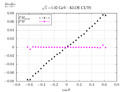
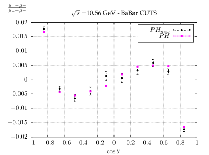
The checks clearly show the control on the numerical accuracy of the virtual corrections. Additionally, using the DT-method and realistic cuts (see Appendix A for their definition) for KLOE and Babar energies, we have studied the relevance of the most challenging contribution in this article. For this purpose, we compare the contributions from one-loop Penta-Box diagrams defined in Section 2 with the Born contributions in Fig. 4.1 for muon angular distributions and in Fig. 4.2 for the $\mu^{+}\mu^{-}$ invariant mass distribution. As we can clearly see from the muon and antimuon angular distributions, the size of the Penta-Box contributions can reach the percent level and they cannot be neglected for the charge odd observables. We confirm here the expectations that the neglected corrections Czyz:2004rj for the charge even distributions are indeed small. For a classification of the charge odd and even contributions, we refer the reader to Ref. Czyz:2003ue , where it was done for charged pions in the final state. Replacing pions with muons does not change the classification presented there.

Figure 4.1: Relevance of NLO Penta-Box contributions at KLOE (above) and Babar (below) energies for muon angular distributions: $\theta_{\mu^{+}}$ is the $\mu^{+}$ polar angle, while $\theta$ is the angle of $\mu^{+}$ or $\mu^{-}$ for the charge ’blind’ observable. These definitions are the same in all the figures and will not be repeated in captions.

Figure 4.2: Relevance of NLO Penta-Box contributions at KLOE (left) and Babar (right) energies for $q^{2}$ $\mu^{+}\mu^{-}$ distributions.

Figure 4.3: On left: Muon pair distributions including 5-point functions at KLOE calculated with PJFry (bottom: absolute error estimate). On right: the same calculated without decicated routines to avoid small Gram determinants. Approximately $4\cdot 10^{10}$ ($10^{9}$) events have been generated.

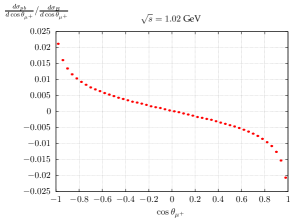
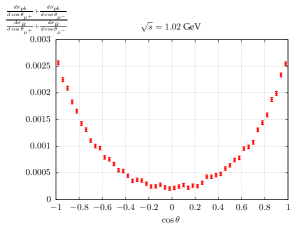
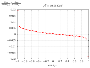
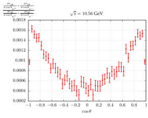
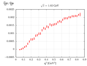
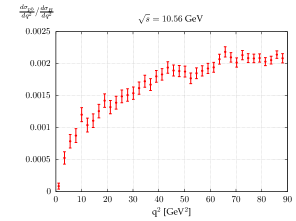
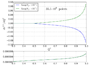
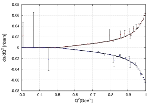
To appreciate these results, in Fig. 4.3, we plot the Penta-Box contributions using the PJFry package with (left) and without (right) using expansion for small Gram determinants. The right panel reveals discrepancies only after increasing the number of Monte Carlo events to $10^{9}$ kajphd ; Gluza:2012yz . PJFry treats properly small Gram determinants, as discussed in details in yundin-phd-2012–oai:export . With the PJFry package, the leading inverse Gram determinants $|G^{(5)}|$ are eliminated in the tensor reduction and small inverse Gram determinants $|G^{(4)}|$ are avoided using asymptotic expansions and Pade approximants. For more details concerning the numerical stability of the tensor reductions, see Refs. yundin-phd-2012–oai:export ; Fleischer:2011bi . The results are completely stable and well under control.

The soft real emission analytic formulae were also checked. Firstly, by comparing to the integral obtained by means of a Monte Carlo methods. A good agreement was found even if the method is limited in some cases to an accuracy of $2\cdot 10^{-4}$. Secondly, the numerical stability of the code was tested comparing the quadruple and the double precision versions of the same code. The relative accuracy of the double precision version used in the released code of the generator is at the level of $10^{-7}$ at 1 GeV, while at 10 GeV , it was only about $10^{-3}$ in some corners of the phase space. However, since those phase space regions did not affect the relevant observables (invariant mass and angular distributions), the code was not changed to cure this behaviour by means of appropriate expansions.

The new contributions of the real two-photon emission were tested comparing two completely independent codes. In one, the trace method (T) and FORM Kuipers:2012rf was used to obtain an analytic result, in the second one, the helicity amplitude method (H), described in Rodrigo:2001kf and in Appendix B, was applied.

The biggest observed relative difference of the codes was at the level of $10^{-4}$ even if both codes were using double precision only. Additionally, in both cases gauge invariance was checked. For the T-method analytically, and for the H-method numerically, obtaining a relative accuracy of $10^{-15}$.

Both the soft and the real parts were tested checking the independence of the cross section and differential distributions of the separation parameter between the soft part, where the integral over the one photon phase space is performed analytically, and the hard part, where the integral is obtained using the Monte Carlo generation. The accuracy of this test was $2\cdot 10^{-4}$. A perfect agreement at this level of accuracy was observed.

5 Impact of the radiative corrections added to the event generator on the pion form factor measurements at BaBar and KLOE

PHOKHARA7.0 has been used by BaBar and KLOE until quite recently. In fact, from version 4.0 to 7.0 the muon production channel was not changed. Comparing numerics with PHOKHARA9.0, which includes the complete NLO corrections, one has to distinguish between the charge average distributions for which the bulk of the NLO corrections was already included in PHOKHARA7.0 and the charge sensitive observables for which version 7.0 was limited to the leading order only. In the experimental framework for the extraction of the hadronic cross section, charge averaged observables were used. The most important invariant muon pair mass distribution (i.e. the $q^{2}$ distribution), from which the hadronic cross section is extracted, is shown in Fig. 5.1. As one can see, the radiative corrections missing in PHOKHARA7.0 are small. They reach up to 0.1 % for the KLOE event selection and up to 0.25% for the BaBar event selection.

(a)

(b)

Figure 5.1: The relative difference between differential cross sections of PHOKHARA7.0 and PHOKHARA9.0 (with subscript ‘new’).

The charge averaged angular distributions are also not very much different as shown in Fig. 5.2 and Fig. 5.3 for different $q^{2}$ bins. For other muon pair invariant mass ranges, the results are similar to the ones shown. We can conclude at this point that in the experiments using the charge averaged observables, the missing radiative corrections are very small and should not have affected the extraction of the hadronic cross section.

Figure 5.2: The relative difference between differential cross sections of PHOKHARA7.0 and PHOKHARA9.0 (with subscript ‘new’). $q^{2}\in(0.54,0.55)$.

Figure 5.3: The relative difference between differential cross sections of PHOKHARA7.0 and PHOKHARA9.0 (with subscript ‘new’). $q^{2}\in(0.94,0.95)$ for KLOE cuts; $q^{2}\in(0.74,0.75)$ for BaBar cuts.

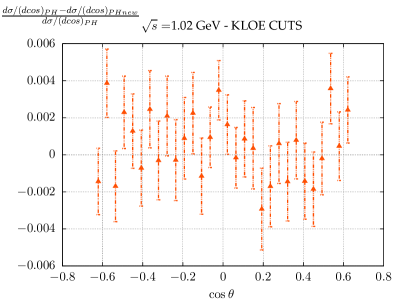
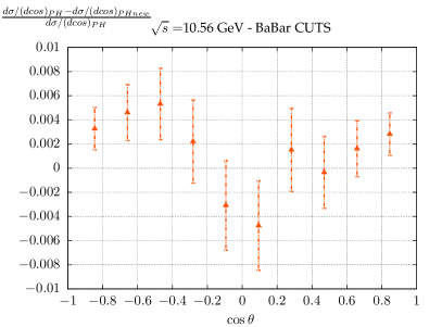
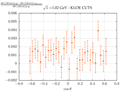
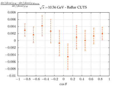
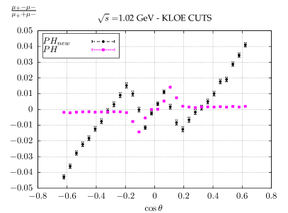
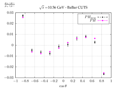
For the charge sensitive observables, which were available at PHOKHARA7.0 only at LO (the ISR-FSR interference was present at LO only) the new corrections are relatively bigger and reach typically a few percent as expected from NLO corrections. The KLOE event selection was designed to diminish the FSR radiative corrections and as such it was also mostly killing the asymmetry coming from one photon emission. The asymmetry coming from the two photon emission is however surviving the cuts as shown in Fig. 5.4. For BaBar, the asymmetry is naturally suppressed by tagging the photon at large angles. At low invariant masses, as compared to the energy available at the experiment, it forces the muons to fly in the opposite direction to the photon and thus the suppression. The asymmetry is at the level of few percent and it is dominated by the LO contributions as shown in Fig. 5.5.

Figure 5.4: The asymmetries given by PHOKHARA7.0 (denoted as $PH$) and PHOKHARA9.0 (denoted as $PH_{new}$). $q^{2}\in(0.54,0.55)$ - left plot; $q^{2}\in(0.94,0.95)$ - right plot.

Figure 5.5: The asymmetries given by PHOKHARA7.0 (denoted as $PH$) and PHOKHARA9.0 (denoted as $PH_{new}$). $q^{2}\in(0.54,0.55)$ - left plot; $q^{2}\in(0.74,0.75)$ - right plot.

6 Conclusions

The presented studies allow for the development of a numerically stable Monte Carlo event generator PHOKHARA9.0 simulating the reaction $e^{+}e^{-}\to\mu^{+}\mu^{-}\gamma$ with full NLO QED accuracy. The radiative corrections which were missing in the previous versions of the generator can reach a few percent. Though, it was shown that the charge blind observables used by the BaBar and KLOE collaborations are affected only at the level of 0.1% for KLOE and 0.3% for BaBar. We conclude that the observed discrepancies between these experiments cannot be attributed to the missing corrections for the reaction $e^{+}e^{-}\to\mu^{+}\mu^{-}\gamma$ in PHOKHARA4.0 Czyz:2004rj ; Czyz:2004ua to PHOKHARA8.0 Czyz:2013xga .

Appendix A KLOE and BaBar event selections cuts

A.1 KLOE

• $\sqrt{s}=1.02$ GeV

• Muon tracks: $50^{\circ}<\theta_{\mu^{\pm}}<130^{\circ}$

• Missing photon angle $<15^{\circ}(>165^{\circ})$

• Track mass: $80$ MeV $<m_{\rm trk}<115$ MeV

• $q^{2}\in(0.34,0.96)$

A.2 BaBar

• $\sqrt{s}=10.56$  GeV

• Muon tracks: $20^{\circ}<\theta_{\mu^{\pm}}<160^{\circ}$

• Minimal photon energy/missing energy 3 GeV

• $|q_{1}|>1$ GeV (antimuon) and $|q_{2}|>1$ GeV (muon)

• $q^{2}\in(0.34,0.96)$

Appendix B Two-hard photon emission

We use here the following notation:

• $p_{1}$ - positron ($e^{+}$) four momenta;

• $p_{2}$ - electron ($e^{-}$) four momenta;

• $q_{1}$ - antimuon ($\mu^{+}$) four momenta;

• $q_{2}$ - muon ($\mu^{-}$) four momenta;

• $k_{1}$, $k_{2}$ - photon four momenta.

The coefficients of the two-hard photon emission amplitude of Eq. 2.3 are given by

$$A\left(\lambda_{1},\lambda_{2}\right)=\frac{-e^{3}}{4s}(\frac{a_{1}\varepsilon^{*-}_{2}a_{3}}{(k_{1}\cdotp q_{1})N_{1}}+\frac{a_{1}\varepsilon^{*-}_{1}a_{5}}{(k_{2}\cdotp q_{1})N_{1}}+\frac{a_{7}\varepsilon^{*-}_{1}a_{9}}{(k_{2}\cdotp q_{2})N_{2}}$$ (B.1)

$$+\frac{a_{11}\varepsilon^{*-}_{2}a_{9}}{(k_{1}\cdotp q_{2})N_{2}}-\frac{a_{7}J_{e^{+}e^{-}}^{-}a_{3}}{(k_{1}\cdotp q_{1})(k_{2}\cdotp q_{2})}-\frac{a_{11}J_{e^{+}e^{-}}^{-}a_{5}}{(k_{2}\cdotp q_{1})(k_{1}\cdotp q_{2})})$$

and

$$B\left(\lambda_{1},\lambda_{2}\right)=\frac{-e^{3}}{4s}(\frac{a_{2}\varepsilon^{*+}_{2}a_{4}}{(k_{1}\cdotp q_{1})N_{1}}+\frac{a_{2}\varepsilon^{*+}_{1}a_{6}}{(k_{2}\cdotp q_{1})N_{1}}+\frac{a_{8}\varepsilon^{*+}_{1}a_{10}}{(k_{2}\cdotp q_{2})N_{2}}$$ (B.2)

$$+\frac{a_{12}\varepsilon^{*+}_{2}a_{10}}{(k_{1}\cdotp q_{2})N_{2}}-\frac{a_{8}J_{e^{+}e^{-}}^{+}a_{4}}{(_{1}\cdotp q_{1})(k_{2}\cdotp q_{2})}-\frac{a_{12}J_{e^{+}e^{-}}^{+}a_{6}}{(k_{2}\cdotp q_{1})(k_{1k}\cdotp q_{2})}),$$

where

$$N_{1} =k_{1}\cdotp q_{1}+k_{2}\cdotp q_{1}+k_{1}\cdotp k_{2}, ~{}~{}~{}~{}~{}~{}N_{2} =k_{1}\cdotp q_{2}+k_{2}\cdotp q_{2}+k_{1}\cdotp k_{2},$$ (B.3)

$$a_{1} =J_{e^{+}e^{-}}^{-}(p_{1}^{+}+p_{2}^{+})-2q_{2}\cdotp J_{e^{+}e^{-}}, ~{}~{}~{}~{}~{}~{}a_{2} =J_{e^{+}e^{-}}^{+}(p_{1}^{-}+p_{2}^{-})-2q_{2}\cdotp J_{e^{+}e^{-}},$$

$$a_{3} =k^{+}_{1}\varepsilon^{*-}_{1}+2(\varepsilon^{*}_{1}\cdotp q_{1}), a_{4} =k^{-}_{1}\varepsilon^{*+}_{1}+2(\varepsilon^{*}_{1}\cdotp q_{1}),$$

$$a_{5} =k^{+}_{2}\varepsilon^{*-}_{2}+2(\varepsilon^{*}_{2}\cdotp q_{1}), a_{6} =k^{-}_{2}\varepsilon^{*+}_{2}+2(\varepsilon^{*}_{2}\cdotp q_{1}),$$

$$a_{7} =\varepsilon^{*-}_{2}k^{+}_{2}+2(\varepsilon^{*}_{2}\cdotp q_{2}), a_{8} =\varepsilon^{*+}_{2}k^{-}_{2}+2(\varepsilon^{*}_{2}\cdotp q_{2}),$$

$$a_{9} =(p_{1}^{+}+p_{2}^{+})J_{e^{+}e^{-}}^{-}-2q_{1}\cdotp J_{e^{+}e^{-}}, a_{10} =(p_{1}^{-}+p_{2}^{-})J_{e^{+}e^{-}}^{+}-2q_{1}\cdotp J_{e^{+}e^{-}},$$

$$a_{11} =\varepsilon^{*-}_{1}k^{+}_{1}+2(\varepsilon^{*}_{1}\cdotp q_{2}), a_{12} =\varepsilon^{*+}_{1}k^{-}_{1}+2(\varepsilon^{*}_{1}\cdotp q_{2}).$$

For the reader’s convenience, we give here all the relevant definitions. The gamma matrices and related objects are defined in the following form:

$$\gamma^{\mu}=\left(\begin{array}[]{cc}0&\sigma^{\mu}_{+}\\ \sigma^{\mu}_{-}&0\end{array}\right)~{},\qquad\mu=0,1,2,3~{},\qquad a/=a_{\mu}\gamma^{\mu}=\left(\begin{array}[]{cc}0&a^{+}\\ a^{-}&0\end{array}\right)~{},$$ (B.8)

$$a^{\pm}=a^{\mu}\sigma_{\mu}^{\pm} =\left(\begin{array}[]{cc}a^{0}\mp a^{3}&\mp(a^{1}-ia^{2})\\ \mp(a^{1}+ia^{2})&a^{0}\pm a^{3}\end{array}\right)~{}.$$ (B.11)

The helicity spinors $u$ and $v$ for a particle and an antiparticle are given by:

$$u(p,\lambda) =\left(\begin{array}[]{c}\sqrt{E-\lambda|{\bf p}|}\;\chi({\bf p},\lambda)\\ \sqrt{E+\lambda|{\bf p}|}\;\chi({\bf p},\lambda)\end{array}\right)\equiv\left(\begin{array}[]{c}u_{I}\\ u_{II}\end{array}\right)~{},$$ (B.16)

$$v(p,\lambda) =\left(\begin{array}[]{c}-\lambda\sqrt{E+\lambda|{\bf p}|}\;\chi({\bf p},-\lambda)\\ \lambda\sqrt{E-\lambda|{\bf p}|}\;\chi({\bf p},-\lambda)\end{array}\right)\equiv\left(\begin{array}[]{c}v_{I}\\ v_{II}\end{array}\right)~{}.$$ (B.21)

Where helicity $\lambda/2=\pm 1/2$.

The helicity eigenstates $\chi({\bf p},\lambda)$ are expressed in terms of the polar and azimuthal angles of the momentum vector ${\bf p}$:

$$\chi({\bf p},+1) =\left(\begin{array}[]{r}\cos{(\theta/2)}\\ e^{i\phi}\sin{(\theta/2)}\end{array}\right)~{},$$ (B.24)

$$\chi({\bf p},-1) =\left(\begin{array}[]{r}-e^{-i\phi}\sin{(\theta/2)}\\ \cos{(\theta/2)}\end{array}\right)~{}.$$ (B.27)

However, for incoming particles in their CMS coordinate frame with z-axis along the positron direction they simplify to:

$$\chi({\bf p_{1}},+1)=\left(\begin{array}[]{r}1\\ 0\end{array}\right)~{},\qquad\chi({\bf p_{1}},-1)=\left(\begin{array}[]{r}0\\ 1\end{array}\right)~{},$$ (B.32)

for positron and

$$\chi({\bf p_{2}},+1)=\left(\begin{array}[]{r}0\\ -1\end{array}\right)~{},\qquad\chi({\bf p_{2}},-1)=\left(\begin{array}[]{r}1\\ 0\end{array}\right)~{},$$ (B.37)

for electron.

The photon polarisation vectors in the helicity basis are defined as

$$\varepsilon^{\mu}(k_{i},\lambda_{i}=\mp)=\frac{1}{\sqrt{2}}\big{(}0,\pm\cos\theta_{i}\cos\phi_{i}+i\sin\phi_{i},\pm\cos\theta_{i}\sin\phi_{i}-i\cos\phi_{i},\mp\sin{\theta_{i}}\big{)}~{},$$ (B.38)

with $i=1,2$.

Appendix C The soft photon integrals

The function $F(p_{1},p_{2},q_{1},q_{2},r)$ defined in 2.1 can be split into three parts

$$F(p_{1},p_{2},q_{1},q_{2},r)=F_{ISR}(p_{1},p_{2},r)+2F_{INT}(p_{1},p_{2},q_{1},q_{2},r)$$

$$+F_{FSR}(q_{1},q_{2},r)$$ (C.1)

with

$$F_{ISR}(p_{1},p_{2},r)=\frac{-\alpha}{4\pi}\int\frac{d^{3}k_{1}}{E_{k_{1}}}\left(\frac{p_{1}}{p_{1}\cdotp k_{1}}-\frac{p_{2}}{k_{1}\cdotp p_{2}}\right)^{2},$$ (C.2)

$$F_{FSR}(q_{1},q_{2},r)=\frac{-\alpha}{4\pi}\int\frac{d^{3}k_{1}}{E_{k_{1}}}\left(\frac{q_{2}}{q_{2}\cdotp k_{1}}-\frac{q_{1}}{k_{1}\cdotp q_{1}}\right)^{2},$$ (C.3)

and

$$F_{INT}(p_{1},p_{2},q_{1},q_{2},r)=\frac{-\alpha}{4\pi}\int\frac{d^{3}k_{1}}{E_{k_{1}}}\left(\frac{p_{1}^{\mu}}{p_{1}\cdotp k_{1}}-\frac{p^{\mu}_{2}}{k_{1}\cdotp p_{2}}\right)\left(\frac{q_{2\mu}}{q_{2}\cdotp k_{1}}-\frac{q_{1\mu}}{k_{1}\cdotp q_{1}}\right).$$ (C.4)

Those parts of the functions $F_{i}$ for $i=ISR,FSR,INT$, which depend explicitly on the ratio of the photon energy cut-off $E_{max}$ and the photon mass regulator $\lambda$ ($r=\frac{2E_{max}}{\lambda}$) are denoted by $F_{ir}$ and read

$$F_{r}(p_{1},p_{2},q_{1},q_{2},r)=F_{ISRr}(p_{1},p_{2},r)+2F_{INTr}(p_{1},p_{2},q_{1},q_{2},r)$$

$$+F_{FSRr}(q_{1},q_{2},r)$$ (C.5)

with

$$F_{ISRr}(p_{1},p_{2},r)=-\frac{2\alpha}{\pi}\left[1-\frac{p_{1}p_{2}\log{\left(\frac{(1+\beta_{e})^{4}}{16m_{e}^{4}/s^{2}}\right)}}{s\beta_{e}}\right]\log{\left(r\right)},$$ (C.6)

$$F_{FSRr}(q_{1},q_{2},r)=-\frac{2\alpha}{\pi}\left[1-\frac{q_{1}q_{2}\log{\left(\frac{(1+\beta_{\mu})^{4}}{16m_{\mu}^{4}/q^{4}}\right)}}{q^{2}\beta_{\mu}}\right]\log{\left(r\right)},$$ (C.7)

$$F_{INTr}(p_{1},p_{2},q_{1},q_{2},r)=-\frac{\alpha}{\pi}\sum^{2}_{i,j=1}\frac{(-1)^{j}p_{i}q_{j}\log{\left(\frac{(1+\beta_{ij})^{2}(p_{i}q_{j})^{2}}{m_{e}^{2}m_{\mu}^{2}}\right)}}{2\sqrt{(p_{i}q_{j})^{2}-m_{e}^{2}m_{\mu}^{2}}}\log{\left(r\right)},\ \$$ (C.8)

and

$$\beta_{i}=\sqrt{1-4m_{i}^{2}/s}$$

$$\beta_{ij}=\sqrt{1-m_{e}^{2}m_{\mu}^{2}/(p_{i}q_{j})^{2}}.$$ (C.9)

Terms proportional to $\frac{\lambda}{E_{max}}$ are neglected. The ’translation’ to dimensional regularisation results in changing

$$\log{\left(\frac{\lambda^{2}}{s}\right)}\quad{\rm into}\quad\Delta=\frac{(4\pi)^{\epsilon}}{\epsilon\Gamma(1-\epsilon)}\left(\frac{\mu^{2}}{s}\right)^{\epsilon}~{}.$$ (C.10)

The remaining parts $F_{i,fin}$ of the soft formula $F_{i}=F_{ir}+F_{i,fin}$ have the following form:

$$F_{ISR,fin}(q_{1},q_{2})=-\frac{\alpha}{4\pi^{2}}(I_{1}(p_{1})+I_{1}(p_{2})-2I_{3}(p_{1},p_{2})),$$ (C.11)

$$F_{FSR,fin}(q_{1},q_{2})=-\frac{\alpha}{4\pi^{2}}(I_{1}(q_{1})+I_{1}(q_{2})-2I_{3}(q_{1},q_{2})),$$ (C.12)

$$F_{INT,fin}(p_{1},p_{2},q_{1},q_{2})=-\frac{4\alpha}{\pi^{2}}\sum^{2}_{i,j=1}(-1)^{j}I_{3}(p_{i},q_{j})).$$ (C.13)

The arguments $x_{i}$ of $I_{1}(x_{1})$ and $I_{3}(x_{1},x_{2})$ are four momenta, $x_{i}=(x_{i}(0),\bar{x_{i}})$:

$$I_{1}(x)=\frac{2\pi x(0)}{|\bar{x}|}\log\left(\frac{x(0)-|\bar{x}|}{x(0)+|\bar{x}|}\right),$$ (C.14)

$$I_{3}(x_{1},x_{2}))=f_{1}(C_{3a}I_{3a}+C_{3b}I_{3b}+C_{3c}I_{3c}+C_{3d}I_{3d}),$$ (C.15)

$$f_{1}(x_{1},x_{2})\equiv f_{1}=\frac{8\pi x_{1}x_{2}(|\bar{x}_{2}-\bar{x}_{1}|)^{3/2}}{|\bar{x}_{1}|^{2}\bar{x}_{2}|^{2}-(\bar{x}_{1}\bar{x}_{2})(x_{2}-x_{1})^{2}}.$$ (C.16)

The $I_{3a}$ function depends on the sign of $f_{1}$. If $f_{1}<0$ then:

$$I_{3a}(x_{1},x_{2})\equiv I_{3a} = \log{\left(\frac{t_{y}t_{3}-1}{t_{x}t_{3}-1}\right)}\log{\left(\frac{C_{2}(t_{4}-t_{3})t_{3}}{(1+t_{3}t_{4})(1+t_{3}^{2})}\right)}$$ (C.17)

$$+~{}\frac{1}{2}\log^{2}{\left(\frac{t_{y}t_{3}-1}{t_{3}}\right)}-\frac{1}{2}\log^{2}{\left(\frac{t_{x}t_{3}-1}{t_{3}}\right)}-\textrm{Li${}_{2}$}\left(\frac{(t_{y}t_{3}-1)t_{4}}{t_{3}-t_{4}}\right)$$

$$+~{}\textrm{Li${}_{2}$}\left(\frac{(t_{x}t_{3}-1)t_{4}}{t_{3}-t_{4}}\right)+\textrm{Li${}_{2}$}\left(\frac{1-t_{3}t_{y}}{1+t_{3}^{2}}\right)-\textrm{Li${}_{2}$}\left(\frac{1-t_{3}t_{x}}{1+t_{3}^{2}}\right)$$

$$+~{}\textrm{Li${}_{2}$}\left(\frac{1-t_{3}t_{y}}{1+t_{3}t_{4}}\right)-\textrm{Li${}_{2}$}\left(\frac{1-t_{3}t_{x}}{1+t_{3}t_{4}}\right)$$

If $f_{1}>0$ then:

$$I_{3a}(x_{1},x_{2})\equiv I_{3a}=\log{\left(\frac{t_{y}t_{3}-1}{t_{x}t_{3}-1}\right)}\log{\left(\frac{C_{2}(t_{4}-t_{3})t_{3}}{(1+t_{3}^{2})}\right)}$$

$$+\frac{1}{2}\log^{2}{\left(\frac{1-t_{y}t_{3}}{t_{3}}\right)}-\frac{1}{2}\log^{2}{\left(\frac{1-t_{x}t_{3}}{t_{3}}\right)}-\textrm{Li${}_{2}$}\left(\frac{(t_{y}t_{3}-1)t_{4}}{t_{3}-t_{4}}\right)$$

$$+\log{\left(\frac{1+t_{3}t_{4}-1}{t_{3}}\right)}\log{\left(\frac{t_{y}+t_{4}}{t_{x}+t_{4}}\right)}-\log{\left(\frac{1-t_{y}t_{3}}{t_{3}}\right)}\log{\left(-t_{y}-t_{4}\right)}$$

$$+\log{\left(\frac{1-t_{x}t_{3}}{t_{3}}\right)}\log{\left(-t_{x}-t_{4}\right)}+\textrm{Li${}_{2}$}\left(\frac{(t_{x}t_{3}-1)t_{4}}{t_{3}-t_{4}}\right)$$

$$+\textrm{Li${}_{2}$}\left(\frac{1-t_{3}t_{y}}{1+t_{3}^{2}}\right)-\textrm{Li${}_{2}$}\left(\frac{1-t_{3}t_{x}}{1+t_{3}^{2}}\right)-\textrm{Li${}_{2}$}\left(\frac{(t_{y}-t_{4})t_{3}}{1+t_{3}t_{4}}\right)$$

$$+\textrm{Li${}_{2}$}\left(\frac{(t_{x}-t_{4})t_{3}}{1+t_{3}t_{4}}\right)$$ (C.18)

$$I_{3b}(x_{1},x_{2})\equiv I_{3b}=\log{\left(\frac{t_{y}t_{4}-1}{t_{x}t_{4}-1}\right)}\log{\left(\frac{C_{2}(t_{3}-t_{4})}{(1+t_{4}^{2})t_{3}}\right)}+\frac{1}{2}\log^{2}{\left(\frac{t_{y}t_{4}-1}{t_{4}}\right)}$$

$$-\frac{1}{2}\log^{2}{\left(\frac{t_{x}t_{4}-1}{t_{4}}\right)}-\log{\left(\frac{t_{y}t_{4}-1}{t_{4}}\right)}\log{\left(t_{y}-t_{3}\right)}$$

$$+\log{\left(\frac{t_{x}t_{4}-1}{t_{4}}\right)}\log{\left(t_{x}-t_{3}\right)}+\log{\left(\frac{-t_{3}t_{4}-1}{t_{4}}\right)}\log{\left(\frac{t_{y}+t_{3}}{t_{x}+t_{3}}\right)}$$

$$-\textrm{Li${}_{2}$}\left(\frac{(1-t_{y}t_{4})t_{4}}{t_{3}-t_{4}}\right)+\textrm{Li${}_{2}$}\left(\frac{(1-t_{x}t_{4})t_{4}}{t_{3}-t_{4}}\right)-\textrm{Li${}_{2}$}\left(\frac{(t_{y}+t_{3})t_{4}}{1+t_{3}t_{4}}\right)$$

$$+\textrm{Li${}_{2}$}\left(\frac{(t_{x}+t_{3})t_{4}}{1+t_{3}t_{4}}\right)+\textrm{Li${}_{2}$}\left(\frac{1-t_{y}t_{4}}{1+t_{4}^{2}}\right)-\textrm{Li${}_{2}$}\left(\frac{1-t_{x}t_{4}}{1+t_{4}^{2}}\right)\ \$$ (C.19)

$$I_{3c}(x_{1},x_{2})\equiv I_{3c}=\log{\left(\frac{t_{y}+t_{3}}{t_{x}+t_{3}}\right)}\log{\left(\frac{C_{2}(1+t_{3}^{2})(1+t_{3}t_{4}}{t_{3}t_{4}(t_{4}-t_{3})}\right)}$$

$$-\frac{1}{2}\log^{2}{\left(t_{y}+t_{3}\right)}+\frac{1}{2}\log^{2}{\left(t_{x}+t_{3}\right)}-\textrm{Li${}_{2}$}\left(\frac{(t_{y}+t_{3})t_{3}}{1+t_{3}^{2}}\right)$$

$$+\textrm{Li${}_{2}$}\left(\frac{(t_{x}+t_{3})t_{3}}{1+t_{3}^{2}}\right)-\textrm{Li${}_{2}$}\left(\frac{(t_{y}+t_{3})t_{4}}{1+t_{3}t_{4}}\right)+\textrm{Li${}_{2}$}\left(\frac{(t_{x}+t_{3})t_{4}}{1+t_{3}t_{4}}\right)$$

$$+\textrm{Li${}_{2}$}\left(\frac{(t_{y}+t_{3})t_{4}}{t_{3}-t_{4}}\right)-\textrm{Li${}_{2}$}\left(\frac{(t_{x}+t_{3})t_{4}}{t_{3}-t_{4}}\right)$$ (C.20)

$$I_{3d}(x_{1},x_{2})\equiv I_{3d}(=-\log{\left(\frac{t_{y}+t_{4}}{t_{x}+t_{4}}\right)}\log{\left(\frac{C_{2}(1+t_{4}^{2})(1+t_{3}t_{4}}{t_{3}t_{4}(t_{4}-t_{3})}\right)}$$

$$+\frac{1}{2}\log^{2}{\left(-t_{y}-t_{4}\right)}-\frac{1}{2}\log^{2}{\left(-t_{x}-t_{4}\right)}+\textrm{Li${}_{2}$}\left(\frac{(t_{y}+t_{4})t_{3}}{1+t_{3}t_{4}}\right)$$

$$-\textrm{Li${}_{2}$}\left(\frac{(t_{x}+t_{4})t_{3}}{1+t_{3}t_{4}}\right)+\textrm{Li${}_{2}$}\left(\frac{(t_{y}+t_{4})t_{4}}{1+t_{4}^{2}}\right)-\textrm{Li${}_{2}$}\left(\frac{(t_{x}+t_{4})t_{4}}{1+t_{4}^{2}}\right)$$

$$-\textrm{Li${}_{2}$}\left(\frac{t_{y}+t_{4}}{t_{4}-t_{3}}\right)+\textrm{Li${}_{2}$}\left(\frac{t_{x}+t_{4}}{t_{4}-t_{3}}\right)$$ (C.21)

$$C_{3a}(x_{1},x_{2})\equiv C_{3a}=\frac{2(x_{2}(0)-x_{1}(0))\sqrt{|\bar{x}_{1}|^{2}|\bar{x}_{2}|^{2}-\bar{x}_{1}\bar{x}_{2}}(t_{3}^{2}-1)}{(|\bar{x}_{1}|^{2}+|\bar{x}_{2}|^{2}-2\bar{x}_{1}\bar{x}_{2})t_{3}^{2}(t_{3}+\frac{1}{t_{3}})(t_{4}+\frac{1}{t_{3}})(\frac{1}{t_{3}}-\frac{1}{t_{4}})}$$

$$+\frac{4(x_{2}(0)-x_{1}(0))(|\bar{x}_{1}|^{2}-\bar{x}_{1}\bar{x}_{2})t_{3}}{(|\bar{x}_{1}|^{2}+|\bar{x}_{2}|^{2}-2\bar{x}_{1}\bar{x}_{2})t_{3}^{2}(t_{3}+\frac{1}{t_{3}})(t_{4}+\frac{1}{t_{3}})(\frac{1}{t_{3}}-\frac{1}{t_{4}})}$$

$$+\frac{4x_{1}(0)}{t_{3}(t_{3}+\frac{1}{t_{3}})(t_{4}+\frac{1}{t_{3}})(\frac{1}{t_{3}}-\frac{1}{t_{4}})}\ \$$ (C.22)

$$C_{3b}(x_{1},x_{2})\equiv C_{3b}=-\frac{2(x_{2}(0)-x_{1}(0))\sqrt{|\bar{x}_{1}|^{2}|\bar{x}_{2}|^{2}-\bar{x}_{1}\bar{x}_{2}}(t_{4}^{2}-1)}{(|\bar{x}_{1}|^{2}+|\bar{x}_{2}|^{2}-2\bar{x}_{1}\bar{x}_{2})t_{4}^{2}(\frac{1}{t_{3}}-\frac{1}{t_{4}})(t_{3}+\frac{1}{t_{4}})(t_{4}+\frac{1}{t_{4}})}$$

$$-\frac{4(x_{2}(0)-x_{1}(0))(|\bar{x}_{1}|^{2}-\bar{x}_{1}\bar{x}_{2})t_{3}}{(|\bar{x}_{1}|^{2}+|\bar{x}_{2}|^{2}-2\bar{x}_{1}\bar{x}_{2})t_{4}^{2}(\frac{1}{t_{3}}-\frac{1}{t_{4}})(t_{3}+\frac{1}{t_{4}})(t_{4}+\frac{1}{t_{4}})}$$

$$-\frac{4x_{1}(0)}{t_{4}(\frac{1}{t_{3}}-\frac{1}{t_{4}})(t_{3}+\frac{1}{t_{4}})(t_{4}+\frac{1}{t_{4}})}\ \$$ (C.23)

$$C_{3c}(x_{1},x_{2})\equiv C_{3c}=\frac{2(x_{2}(0)-x_{1}(0))\sqrt{|\bar{x}_{1}|^{2}|\bar{x}_{2}|^{2}-\bar{x}_{1}\bar{x}_{2}}(t_{3}^{2}-1)}{(|\bar{x}_{1}|^{2}+|\bar{x}_{2}|^{2}-2\bar{x}_{1}\bar{x}_{2})(t_{3}+\frac{1}{t_{3}})(t_{3}+\frac{1}{t_{4}})(t_{3}-t_{4})}$$

$$+\frac{4(x_{2}(0)-x_{1}(0))(|\bar{x}_{1}|^{2}-\bar{x}_{1}\bar{x}_{2})t_{3}}{(|\bar{x}_{1}|^{2}+|\bar{x}_{2}|^{2}-2\bar{x}_{1}\bar{x}_{2})(t_{3}+\frac{1}{t_{3}})(t_{3}+\frac{1}{t_{4}})(t_{3}-t_{4})}$$

$$+\frac{4x_{1}(0)t_{3}}{(t_{3}+\frac{1}{t_{3}})(t_{3}+\frac{1}{t_{4}})(t_{3}-t_{4})}\ \$$ (C.24)

$$C_{3d}(x_{1},x_{2})\equiv C_{3d}=\frac{2(x_{2}(0)-x_{1}(0))\sqrt{|\bar{x}_{1}|^{2}|\bar{x}_{2}|^{2}-\bar{x}_{1}\bar{x}_{2}}(1-t_{4}^{2})}{(|\bar{x}_{1}|^{2}+|\bar{x}_{2}|^{2}-2\bar{x}_{1}\bar{x}_{2})(t_{4}+\frac{1}{t_{3}})(t_{4}+\frac{1}{t_{4}})(t_{3}-t_{4})}$$

$$-\frac{4(x_{2}(0)-x_{1}(0))(|\bar{x}_{1}|^{2}-\bar{x}_{1}\bar{x}_{2})t_{4}}{(|\bar{x}_{1}|^{2}+|\bar{x}_{2}|^{2}-2\bar{x}_{1}\bar{x}_{2})(t_{4}+\frac{1}{t_{3}})(t_{4}+\frac{1}{t_{4}})(t_{3}-t_{4})}$$

$$-\frac{4x_{1}(0)t_{4}}{(t_{4}+\frac{1}{t_{3}})(t_{4}+\frac{1}{t_{4}})(t_{3}-t_{4})}\ \$$ (C.25)

$$t_{x}(x_{1},x_{2})\equiv t_{x}=\frac{|\bar{x}_{1}|^{2}-\bar{x}_{1}\bar{x}_{2}+|\bar{x}_{1}||\bar{x}_{1}-\bar{x}_{2}|}{\sqrt{|\bar{x}_{1}|^{2}|\bar{x}_{1}|^{2}-(\bar{x}_{1}\bar{x}_{2})^{2}}}$$ (C.26)

$$t_{y}(x_{1},x_{2})\equiv t_{y}=\frac{2\bar{x}_{1}\bar{x}_{2}-|\bar{x}_{1}|^{2}-|\bar{x}_{2}|^{2}+|\bar{x}_{2}||\bar{x}_{1}+\bar{x}_{2}|}{\sqrt{|\bar{x}_{1}|^{2}|\bar{x}_{1}|^{2}-(\bar{x}_{1}\bar{x}_{2})^{2}}}$$ (C.27)

$$t_{3,4}(x_{1},x_{2})\equiv t_{3,4}=\frac{x_{1}(0)(|\bar{x}_{2}|^{2}-\bar{x}_{1}\bar{x}_{2})+x_{2}(0)(|\bar{x}_{1}|^{2}-\bar{x}_{1}\bar{x}_{2})\mp\sqrt{\Delta}}{\sqrt{|\bar{x}_{1}|^{2}|\bar{x}_{2}|^{2}-(\bar{x}_{1}\bar{x}_{2})^{2}}((x_{2}(0)-x_{1}(0))+|\bar{x}_{2}-\bar{x}_{1}|)}$$ (C.28)

$$\Delta=(x_{1}(0)(|\bar{x}_{2}|^{2}-\bar{x}_{1}\bar{x}_{2})+x_{2}(0)(|\bar{x}_{1}|^{2}-\bar{x}_{1}\bar{x}_{2}))^{2}$$ (C.29)

$$+(|\bar{x}_{1}|^{2}|\bar{x}_{2}|^{2}-(\bar{x}_{1}\bar{x}_{2})^{2})(x_{2}-x_{1})^{2}$$

$$C_{2}=\frac{(x_{2}-x_{1})^{2}}{(x_{2}(0)-x_{1}(0)+|\bar{x}_{2}-\bar{x}_{1}|)^{2}}.$$ (C.30)

References

- (1) Working Group on Radiative Corrections and Monte Carlo Generators for Low Energies, S. Actis et al., Quest for precision in hadronic cross sections at low energy: Monte Carlo tools vs. experimental data, Eur. Phys. J. C66 (2010) 585–686, [arXiv:0912.0749].
- (2) K. Hagiwara, R. Liao, A. D. Martin, D. Nomura, and T. Teubner, and re-evaluated using new precise data, J. Phys. G38 (2011) 085003, [arXiv:1105.3149].
- (3) M. Davier, A. Hoecker, B. Malaescu, and Z. Zhang, Reevaluation of the hadronic contributions to the muon g-2 and to , Eur. Phys. J. C71 (2011) 1515, [arXiv:1010.4180].
- (4) F. Jegerlehner and A. Nyffeler, The muon g-2, Phys. Rept. 477 (2009) 1–110, [arXiv:0902.3360].
- (5) R. V. Harlander and M. Steinhauser, rhad: A program for the evaluation of the hadronic R ratio in the perturbative regime of QCD, Comput. Phys. Commun. 153 (2003) 244–274, [hep-ph/0212294].
- (6) G. Venanzoni for the Fermilab E989 Collaboration, The new g-2 experiment at Fermilab, talk held at “Dark Forces at Accelerators” (DARK2012), 16-19 Oct 2012, Frascati, Italy, Frascati Phys. Ser. 56 (2012) 195-204, [http://www.lnf.infn.it/sis/frascatiseries/Volume56/Venanzoni.pdf].
- (7) BaBar Collaboration, J. Lees et al., Precise Measurement of the Cross Section with the Initial-State Radiation Method at BABAR, Phys.Rev. D86 (2012) 032013, [arXiv:1205.2228].
- (8) BaBar Collaboration, B. Aubert et al., Precise measurement of the e+ e- -> pi+ pi- (gamma) cross section with the Initial State Radiation method at BABAR, Phys.Rev.Lett. 103 (2009) 231801, [arXiv:0908.3589].
- (9) KLOE Collaboration, D. Babusci et al., Precision measurement of and determination of the contribution to the muon anomaly with the KLOE detector, Phys.Lett. B720 (2013) 336–343, [arXiv:1212.4524].
- (10) KLOE Collaboration, F. Ambrosino et al., Measurement of sigma(e+ e- -> pi+ pi-) from threshold to 0.85 using Initial State Radiation with the KLOE detector, Phys.Lett. B700 (2011) 102–110, [arXiv:1006.5313].
- (11) KLOE Collaboration, F. Ambrosino et al., Measurement of sigma(e + e- -> pi+ pi- gamma(gamma) and the dipion contribution to the muon anomaly with the KLOE detector, Phys.Lett. B670 (2009) 285–291, [arXiv:0809.3950].
- (12) H. Czyz, A. Grzelinska, J. H. Kühn, and G. Rodrigo, The radiative return at and factories: Small angle photon emission at next-to-leading order, Eur. Phys. J. C27 (2003) 563–575, [hep-ph/0212225].
- (13) H. Czyz, A. Grzelinska, J. H. Kühn, and G. Rodrigo, Electron-positron annihilation into three pions and the radiative return, Eur. Phys. J. C47 (2006) 617–624, [hep-ph/0512180].
- (14) P. Khiem, J. Fujimoto, T. Ishikawa, T. Kaneko, K. Kato, et al., Full electroweak radiative corrections to with GRACE-Loop, Eur.Phys.J. C73 (2013) 2400, [arXiv:1211.1112].
- (15) K. Kajda, T. Sabonis, and V. Yundin, QED Pentagon Contributions to , Acta Phys. Polon. B40 (2009) 3127. [APPv40p3127].
- (16) K. Kajda, Multipoint Feynman diagrams at the one-loop level, Ph.D. thesis, Uniwersytet Śla̧ski w Katowicach, 3 Sep 2009, [http://prac.us.edu.pl/~ztpce/materialy/phdKajda.pdf].
- (17) V. Yundin, Massive loop corrections for collider physics, PhD thesis, Humboldt-Universität zu Berlin, 2012, see http:// edoc.hu-berlin.de/docviews/abstract.php?id=39163 and urn:nbn:de:kobv:11-100199626.
- (18) S. Actis, P. Mastrolia, and G. Ossola, Numerical evaluation of one-loop scattering amplitudes for hard-photon emission in Bhabha scattering, Acta Phys. Polon. B40 (2009) 2957. [APPv40p2957].
- (19) S. Actis, P. Mastrolia, and G. Ossola, NLO QED Corrections to Hard-Bremsstrahlung Emission in Bhabha Scattering, Phys. Lett. B682 (2010) 419–427, [arXiv:0909.1750].
- (20) G. ’t Hooft and M. Veltman, Regularization and Renormalization of Gauge Fields, Nucl.Phys. B44 (1972) 189–213, doi:10.1016/0550–3213(72)90279–9.
- (21) M. Böhm, H. Spiesberger, and W. Hollik, On the 1-loop renormalization of the electroweak standard model and its application to leptonic processes, Fortsch. Phys. 34 (1986) 687–751. [10.1002/prop.19860341102].
- (22) A. Denner, Techniques for calculation of electroweak radiative corrections at the one loop level and results for W physics at LEP-200, Fortsch.Phys. 41 (1993) 307–420, [arXiv:0709.1075].
- (23) H. Czyz, A. Grzelinska, and J. H. Kühn, Narrow resonances studies with the radiative return method, Phys. Rev. D81 (2010) 094014, [arXiv:1002.0279].
- (24) V. Yundin, C++ package PJFry. Available at https://github.com/Vayu/PJFry/.
- (25) F. Campanario, Towards pp VVjj at NLO QCD: Bosonic contributions to triple vector boson production plus jet, JHEP 1110 (2011) 070, 10.1007/JHEP10(2011)070.
- (26) P. Nogueira, Automatic Feynman graph generation, J. Comput. Phys. 105 (1993) 279–289, 10.1006/jcph.1993.1074.
- (27) M. Tentyukov and J. Fleischer, A Feynman diagram analyser DIANA, Comput. Phys. Commun. 132 (2000) 124–141, [hep-ph/9904258].
- (28) M. Tentyukov and J. Fleischer, DIANA, a program for Feynman diagram evaluation, talk held at AIHENP 99, 12-16 April 1999, Heraklion, Crete, Greece [hep-ph/9905560].
- (29) J. Vermaseren, New features of FORM, math-ph/0010025.
- (30) G. Passarino and M. Veltman, One Loop Corrections for e+ e- Annihilation Into mu+ mu- in the Weinberg Model, Nucl.Phys. B160 (1979) 151.
- (31) A. I. Davydychev, A simple formula for reducing Feynman diagrams to scalar integrals, Phys. Lett. B263 (1991) 107–111. doi:10.1016/0370-2693(91)91715-8.
- (32) O. Tarasov, Connection between Feynman integrals having different values of the space-time dimension, Phys. Rev. D54 (1996) 6479–6490, [hep-th/9606018].
- (33) J. Fleischer, F. Jegerlehner, and O. Tarasov, Algebraic reduction of one-loop Feynman graph amplitudes, Nucl. Phys. B566 (2000) 423–440, [hep-ph/9907327].
- (34) T. Diakonidis, J. Fleischer, J. Gluza, K. Kajda, T. Riemann, and B. Tausk, A Complete reduction of one-loop tensor 5 and 6-point integrals, Phys. Rev. D80 (2009) 036003, [arXiv:0812.2134].
- (35) T. Diakonidis, J. Fleischer, T. Riemann, and J. Tausk, A recursive reduction of tensor Feynman integrals, Phys. Lett. B683 (2010) 69–74, [arXiv:0907.2115].
- (36) J. Fleischer and T. Riemann, A complete algebraic reduction of one-loop tensor Feynman integrals, Phys. Rev. D83 (2011) 073004, [arXiv:1009.4436].
- (37) A. A. Almasy, I. Dubovyk, J. Gluza, and T. Riemann, Reductions and Contractions of 1-loop Tensor Feynman Integrals, arXiv:1311.2267.
- (38) J. Fleischer, T. Riemann and V. Yundin, PJFry: A C++ package for tensor reduction of one-loop Feynman integrals, preprint DESY 11-252, in: AlcarazMaestre:2012vp-2 .
- (39) R. K. Ellis and G. Zanderighi, Scalar one-loop integrals for QCD, JHEP 02 (2008) 002, [0712.1851].
- (40) G. J. van Oldenborgh, FF: A package to evaluate one loop Feynman diagrams, Comput. Phys. Commun. 66 (1991) 1–15. doi:10.1016/0010-4655(91)90002-3, scanned version at http://ccdb3fs.kek.jp/cgi-bin/img_index?9004168.
- (41) A. van Hameren, OneLOop: For the evaluation of one-loop scalar functions, Comput. Phys. Commun. 182 (2011) 2427–2438, [1007.4716].
- (42) A. Almasy, I. Dubovyk, J. Fleischer, J. Gluza, M. Gluza, and T. Riemann, OLEC project; C++, F99 and Mathematica packages OLEC v.0.9 available at Silesian Univ. , Katowice, webpage http://prac.us.edu.pl/gluza/olec/.
- (43) J. Fleischer, J. Gluza, M. Gluza, T. Riemann, and R. Sevillano, Efficient contraction of 1-loop N-point tensor integrals, PoS LL2012 (2012) 051, [arXiv:1211.3921].
- (44) J. Fleischer and T. Riemann, Calculating contracted tensor Feynman integrals, Phys. Lett. B701 (2011) 646–653, [1104.4067].
- (45) A. Sirlin, A Class of Useful Identities Involving Correlated Direct Products of Matrices, Nucl.Phys. B192 (1981) 93.
- (46) A. Denner and S. Dittmaier, Reduction schemes for one-loop tensor integrals, Nucl. Phys. B734 (2006) 62–115, [hep-ph/0509141].
- (47) T. Binoth, J. P. Guillet, G. Heinrich, E. Pilon, and C. Schubert, An Algebraic/numerical formalism for one-loop multi-leg amplitudes, JHEP 0510 (2005) 015, [hep-ph/0504267].
- (48) G. ’t Hooft and M. Veltman, Scalar One Loop Integrals, Nucl.Phys. B153 (1979) 365–401.
- (49) G. Rodrigo, H. Czyz, J. H. Kühn, and M. Szopa, Radiative return at NLO and the measurement of the hadronic cross-section in electron positron annihilation, Eur. Phys. J. C24 (2002) 71–82, [hep-ph/0112184].
- (50) H. Czyz, A. Grzelinska, J. H. Kuhn, and G. Rodrigo, The Radiative return at phi and B factories: FSR for muon pair production at next-to-leading order, Eur.Phys.J. C39 (2005) 411–420, [hep-ph/0404078].
- (51) F. A. Berends, W. van Neerven, and G. Burgers, Higher Order Radiative Corrections at LEP Energies, Nucl.Phys. B297 (1988) 429, [10.1016/0550–3213(88)90313–6.
- (52) G. Rodrigo, M. S. Bilenky, and A. Santamaria, Quark mass effects for jet production in e+ e- collisions at the next-to-leading order: Results and applications, Nucl.Phys. B554 (1999) 257–297, [hep-ph/9905276].
- (53) M. Gunia, Radiative corrections and accuracy tests of Monte Carlo generators used at meson factories. PhD thesis, University of Silesia, 2013. in preparation.
- (54) H. Czyz, A. Grzelinska, J. H. Kühn, and G. Rodrigo, The radiative return at and factories: FSR at next-to-leading order, Eur. Phys. J. C33 (2004) 333–347, [hep-ph/0308312].
- (55) J. Gluza, M. Gunia, T. Riemann, and M. Worek, Theoretical Improvements for Luminosity Monitoring at Low Energies, PoS RADCOR2011 (2011) 034, [arXiv:1201.0968].
- (56) J. Fleischer, T. Riemann, and V. Yundin, One-Loop Tensor Feynman Integral Reduction with Signed Minors, J. Phys. Conf. Ser. 368 (2012) 012057, [arXiv:1112.0500].
- (57) J. Kuipers, T. Ueda, J. Vermaseren, and J. Vollinga, FORM version 4.0, Comput. Phys. Commun. 184 (2013) 1453–1467, [arXiv:1203.6543].
- (58) H. Czyz, J. H. Kühn, E. Nowak, and G. Rodrigo, Nucleon form-factors, B meson factories and the radiative return, Eur. Phys. J. C35 (2004) 527–536, [hep-ph/0403062].
- (59) H. Czyz, M. Gunia, and J. Kühn, Simulation of electron-positron annihilation into hadrons with the event generator PHOKHARA, JHEP 1308 (2013) 110, [arXiv:1306.1985].
- (60) J. Alcaraz Maestre et al., “The SM and NLO Multileg and SM MC Working Groups: Summary Report.” Report of the SM and NLO Multileg and SM MC Working Groups for the Workshop ’Physics at TeV Colliders’, Les Houches, France, 31 May – 8 June, 2011. See [arXiv:1203.1488] and [arXiv: 1203.6803].