Iterative Hard Thresholding for Weighted Sparse Approximation
Abstract
Recent work by Rauhut and Ward developed a notion of weighted sparsity and a corresponding notion of Restricted Isometry Property for the space of weighted sparse signals. Using these notions, we pose a best weighted sparse approximation problem, i.e. we seek structured sparse solutions to underdetermined systems of linear equations. Many computationally efficient greedy algorithms have been developed to solve the problem of best -sparse approximation. The design of all of these algorithms employ a similar template of exploiting the RIP and computing projections onto the space of sparse vectors. We present an extension of the Iterative Hard Thresholding (IHT) algorithm to solve the weighted sparse approximation problem. This IHT extension employs a weighted analogue of the template employed by all greedy sparse approximation algorithms. Theoretical guarantees are presented and much of the original analysis remains unchanged and extends quite naturally. However, not all the theoretical analysis extends. To this end, we identify and discuss the barrier to extension. Much like IHT, our IHT extension requires computing a projection onto a non-convex space. However unlike IHT and other greedy methods which deal with the classical notion of sparsity, no simple method is known for computing projections onto these weighted sparse spaces. Therefore we employ a surrogate for the projection and present its empirical performance on power law distributed signals.
1 Introduction
Compressed sensing algorithms attempt to solve underdetermined linear systems of equations by seeking structured solutions, namely that the underlying signal is either sparse or well approximated by a sparse signal [1]. However, in practice much more knowledge about a signal’s support set is known beyond that of sparsity or compressibility. Empirically it has been shown that the spectral power of natural images decays with frequency according to a power-law for [2, 3]. Likewise, the frequency of earthquakes corresponding to their magnitudes as measured by Moment magnitude scale empirically also exhibits a power law decay [4]. For these types of highly structured signals, certain atoms in the dictionary are more prevalent in the support set of a signal than other atoms. The traditional notion of sparsity treats all atoms uniformly and thus is not ideally suited to utilize this rich prior knowledge.
To this end one can consider using weighted minimization to obtain structured sparse solutions. Weighted minimization can leverage prior knowledge of a signal’s support to undersample the signal, and avoid overfitting the data [5, 6, 7, 8]. However, one drawback that weighted minimization shares with minimization is that traditional solution methods scale poorly [9].
While many computationally efficient approximation algorithms have been developed for computing a best -sparse approximation [1] no such method has been developed for the weighted case. In this article, we make the following contributions:
-
1.
Using a generalized notion of weighted sparsity and a corresponding notion of Restricted Isometry Property on weighted sparse signals developed in [5], we pose a weighted analogue of the best -sparse approximation problem.
-
2.
An extension of the Iterative Hard Thresholding (IHT) algorithm [10] is presented to solve the weighted sparse approximation problem. We emphasize how the same template used to derive performance guarantees for all the greedy compressed sensing algorithms carries over naturally. Indeed, performance guarantees are derived and much of the theoretical analysis remains unchanged. However, not all theoretical results extend and the barrier seems to be the nature of weighted thresholding. We explore this extension barrier and present a detailed analysis of which theoretical guarantees do not extend and how the barrier is responsible for this obstruction. Under an additional hypothesis, the extension barrier is rendered moot and we present some specialized theoretical guarantees. The nature and proof of these guarantees are all directly motivated by [5].
-
3.
While both IHT and the IHT extension compute a projection onto a non-convex space, the projection that IHT requires can actually be efficiently computed while the projection that our IHT extension requires does not seem to have an efficient solution. To this end, we consider a tractable surrogate to approximate this non-convex projection and we present its empirical performance on power law distributed signals.
The remainder of the article is organized as follows. In Section 2 we quote much of the weighted sparsity concepts developed from [5] that will be needed for the IHWT extension. In Section 3 the IHWT algorithm is presented and theoretical performance guarantees are established. In Section 4 we present various numerical results.
2 Weighted Sparsity
In this section, all of the concepts and definitions are taken from [5]. For unstructured sparse recovery problems, the sparsity of a signal is defined to be the cardinality of its support set, denoted as . More generally, we have a dictionary of atoms and for the unstructured case, each atom is given the weight for all . In this context, the sparsity of a signal can be viewed as the sum of the weights of the atoms in the support set. Following [5], given a dictionary and a corresponding set of weights for , we can define the weighted norm:
Observe that the weighted sparsity of a vector is at least as large as the unweighted sparsity of , i.e. .
For any subset , we may define the weighted cardinality of via:
In general, we also have the weighted spaces with norm:
Using this generalized notion of sparsity allows us to pose the best -sparse approximation problem:
| (1) |
Given this generalized notion of sparsity, [5] defines a generalized notion of a map being an isometry on the space of weighted sparse vectors:
Definition 2.1.
(Weighted restricted isometry constants) For , weight parameter and , the weighted restricted isometry constant associated to is the smallest number for which
holds for all with . We say that a map has the weighted restricted isometry property with respect to the weights (-RIP) if is small for reasonably large compared to .
Observe that for any positive number , there exists a partition of with distinct parts of maximal cardinality, i.e. an index set with -weighted cardinality with the largest number of non-zero atoms. Let denote this maximal term
Clearly if satisfies RIP of order , then will also satisfy the -RIP of order . However the converse does not hold. Not only do weighted sparse signals have a constraint on the cardinality of their support sets, they can also have a constraint on the maximal atom which can be present in their support sets. Take for example the weights defined by , . An -sparse signal cannot have any atom with index higher than supported. If were to satisfy the -RIP of order , then the -RIP alone does not guarantee that preserves the geometry of heavy-tailed signals, no matter how sparse they may be in the unweighted sense. We conclude that the -RIP is in general a weaker isometry condition than the RIP and the primary reason being the existence of heavy tailed signals.
In [5] a heuristic justification is given that for weights satisfying , with high probability an i.i.d. subgaussian random matrix satisfies the -RIP once
Note that fewer measurements are required than in the unweighted case, which has the lower bound of measurements.
The following properties of RIP matrices carry over immediately to -RIP matrices.
Lemma 2.2.
Let denote the identity matrix. Given a set of weights , vectors , and an index set ,
Proof.
The proofs follow immediately from their unweighted counterparts where one employs the -RIP instead of the RIP. See [1] for full proofs. ∎
3 Iterative Hard Weighted Thresholding: In Theory
3.1 Intuition and Background
First we revisit the unweighted case to build some intuition and use it to motivate modifications for the weighted case. In compressed sensing, greedy algorithms solve problems of the form:
where is some structured space and denotes a loss function which depends on and the vector of linear samples , where represents measurement noise and is a sampling matrix. For the case of best -sparse approximation and .
Iterative greedy algorithms such as IHT exploit the RIP in the following manner. If the matrix satisfies the RIP of order , then is a good enough approximation to the identity matrix on the space of -sparse vectors so that applying to the vector of noisy samples approximately yields the true signal up to some “noise term”
Iterative greedy algorithms produce a dense signal approximation at each stage and they denoise this dense signal to output an -sparse approximation. Roughly speaking, the denoising process of all of these iterative methods involves a projection onto the space of sparse vectors. The idea behind this is that while the noise term is dense, its energy is assumed to be spread throughout all of its coordinates and as a result does not heavily contaminate the -most significant coordinates of . Despite the fact that is non-convex, it is very simple to compute projections onto this space: all that is required is sorting the entries of the signal by their magnitude and picking the top entries. This fact combined with the above RIP intuition explains why greedy methods such as IHT can efficiently solve a non-convex problem.
Setting our initial approximation , IHT is the iteration:
| (2) |
where is the hard thresholding operator and at each step it outputs the best -sparse approximation to by projecting it onto . More specifically
| (3) |
Note that by plugging in for , we obtain the following approximation:
Denoising by applying the hard thresholding operator yields , an -sparse approximation to the true underlying signal .
3.2 Extension to the Weighted Case
Observe that one can equivalently view IHT as a projected gradient descent algorithm with constant step size equal to 1. Once IHT is viewed in this manner, the modification we make to extend IHT to solve (1) is quite natural: we still perform a constant step size gradient descent step at each iterate, however instead of projecting onto the space of -sparse vectors, we project onto the space of weighted sparse vectors . This algorithm will be referred to as Iterative Hard Weighted Thresholding (IHWT) and it is given by the following iteration
| (4) |
where is the hard weighted thresholding operator and it computes projections onto the space of weighted sparse vectors
| (5) |
Computing the projection is not as straightforward as computing . In particular, sorting the signal by the magnitude of its entries and then thresholding does not produce the best -sparse approximation. To see why, consider the simple example where and take the signal . For , by sorting and thresholding, we obtain the following weighted 3 sparse approximation and . However, the other 3 sparse approximation is in fact a more accurate weighted 3 sparse approximation as .
Therefore unlike the unweighted case, computing the best weighted -sparse approximation consists of a combinatorial search. To illustrate the difficulty of executing this search, consider the case of a weight parameter given by for . In this case, computing all the possible index sets of weighted cardinality is equivalent to computing all the partitions of consisting of unique parts. With the square root weight parameter, Wolfram Mathematica [11] computes that there are 444,794 possible subsets of weighted sparsity and it computes that there are 8,635,565,795,744,155,161,506 support sets of size .
Despite this intractability, in the next subsection we derive theoretical guarantees for the IHWT algorithm and in Section 4, we will explore the empirical performance of a surrogate to approximate the projection onto .
3.3 Performance Guarantees
Throughout this subsection, we will employ the following notation:
-
1.
as defined by (5),
-
2.
,
-
3.
,
-
4.
,
-
5.
,
-
6.
,
-
7.
.
3.3.1 Performance Guarantees: Convergence to a Neighborhood
Here we derive performance guarantees which establish that IHWT will converge to a neighborhood of the best -sparse approximation with a linear convergence rate. The size of the neighborhood is dependent on how well the true signal is approximated by .
In [10], the following performance guarantee was established 111We use different notation than that of the original authors Blumensath and Davies.:
Theorem 3.1.
Let denote a set of noisy observations where is an arbitrary vector. Let be an approximation to with no more than non-zero elements for which is minimal. If has restricted isometry property with , then at iteration , IHT as defined by (2) will recover an approximation satisfying
| (6) |
where
| (7) |
In other words, IHT guarantees a linear convergence rate up to the unrecoverable energy . This term is referred to as unrecoverable energy as it contains the measurement noise and energy terms which measure how well a signal can be approximated by sparse signals.
We reverse course and instead focus our attention on an intermediate, yet more general error bound for IHT:
Theorem 3.2.
Let denote a set of noisy observations where is an arbitrary vector. Let be an approximation to with no more than non-zero elements for which is minimal. If has restricted isometry property with , then at iteration , IHT as defined by (2) will recover an approximation satisfying
| (8) |
To pass from (8) to (6)–(7), Blumensath and Davies used the following energy bound for RIP matrices from [12]:
Proposition 3.3.
Suppose that verifies the upper inequality
Then, for every signal ,
| (9) |
The proof of Proposition 3.3 boils down to establishing an inclusion of polar spaces: . is equipped with the following norm
The proof proceeds by considering any element of the unit ball in . We decompose into two components: and where represents the best -sparse approximation to in the norm. As contains the most energetic atoms, this implies that the set contains atoms whose energy must lie under a certain threshold: the bound is easily obtained. In other words, the following decomposition is obtained:
and the space on the right hand side is exactly the space . For further details, consult [12], in this article we will only be concerned with this particular aspect of their proof.
This sort of decomposition does not hold for the weighted case. Consider the example in which the weight vector is such that . As mentioned before, with such a weight vector , any sparse signal cannot have any atom of index higher than supported. Therefore, taking the best -sparse approximation to a signal does not constrain the norm of the signal on the complement . As a result of this, Proposition 3.3 does not extend to the weighted case and an alternative method will be needed to bound the energy of . Here we see a key difference between unweighted sparsity and weighted sparsity: significant amounts of energy can be concentrated in the tail . More specifically we see that certain weight vectors can yield the process of taking the best -sparse approximation to be an operation which is inherently local as it may restrict the analysis to lie on a subset of low weight atoms and the higher weight atoms are completely ignored.
An alternative method of bounding the term involves a different type of decomposition. Suppose satisfies the RIP of order with RIP constant . Let be a partition of into -sparse blocks: each satisfies: for all and . We may apply the RIP to each block to obtain the following bound:
This sort of argument in general will not extend to the weighted case. Depending on the weight vector such a decomposition of an arbitrary signal into a collection of disjoint -sparse blocks may not even be possible.
Therefore, the performance guarantee given in Theorem 3.1 does not directly extend to the weighted case. The more general guarantee of Theorem 3.2 however, does extend, and the proof is identical to the proof in the unweighted case.
Theorem 3.4.
Let denote a weight vector with for all . Let denote a set of noisy observations where is an arbitrary vector. If has weighted restricted isometry property with , then at iteration , IHWT as defined by (4) will recover an approximation satisfying
| (10) |
Proof.
We follow the proof presented in [10]. By the triangle inequality we have that:
| (11) |
We focus on the term . This term is supported on and we may therefore restrict our analysis to this index set. By the triangle inequality we have:
By definition of the thresholding operator , the signal is the best weighted sparse approximation to . In particular, is a better weighted sparse approximation to than . We therefore obtain the inequality:
Expanding the term :
Note that is disjoint from and . Applying the RIP bounds from 2.2:
If we have that , then
Iterating this relationship and using the fact that , we obtain the bound:
| (12) |
Note that the proof has two main components: the hard thresholding operator produces , a superior sparse approximation to the gradient descent update than and applying the RIP. Moreover, the proof never requires any details of the projection or even the space we are projecting onto, unlike the proof of Proposition 3.3, which uses special properties of the projection onto the space of unweighted sparse signals. This is precisely why the IHWT performance guarantee and its corresponding analysis is nearly identical to the IHT guarantee from Theorem 3.2.
The existence of weights which are known to produce signals with heavy tails is the main blockage to the extension of some more detailed performance guarantees, like that of Theorem 3.2. In the two cases before, one notices that the existence of heavy tailed signals prevented a decomposition of a signal amenable to further analysis. However, for certain bounded weight parameters, for arbitrary signals , one may obtain a modified bound on in terms of weighted norms. Indeed we obtain the following weighted analogue of Proposition 3.3:
Proposition 3.5.
Consider a sparsity level and a weight parameter satisfying . If satisfies the -RIP of order with RIP constant , then the following inequality holds for any arbitrary signal :
| (13) |
Proof.
The proof employs the same strategy used in the proof of Theorem 4.5 in [5]. Let . We will partition into weighted sparse blocks for some index with each block satisfying . Furthermore, we assume that the blocks are formed according to a nonincreasing rearrangement of with respect to the weights, i.e.
| (14) |
For any , set by hypothesis. Notice that . For then:
| (15) | ||||
| (16) | ||||
| (17) | ||||
| (18) |
where (15) holds by nonincreasing rearrangement and convexity and (16) holds by hypothesis. Therefore, by the Cauchy-Schwarz inequality, we obtain:
For , we obtain the following estimate:
∎
Applying 3.5 to immediately yields the following performance bound:
Theorem 3.6.
For sparsity level , let denote a weight vector with for all satisfying . Let denote a set of noisy observations where is an arbitrary vector. If has weighted restricted isometry property with , then at iteration , IHWT as defined by (4) will recover an approximation satisfying
| (19) |
This result bears a striking resemblance to Theorem 3.1 except that it is in terms of the weighted norm as opposed to the unweighted norm.
3.3.2 Performance Guarantees: Contraction
For an arbitrary, possibly dense signal , the performance guarantees presented above do not guarantee the convergence of IHT/IHWT, but rather they guarantee that if the sampling matrix satisfies the RIP of order then the iterates are guaranteed to converge to a neighborhood of the true best -sparse approximation. In [13], alternative guarantees are derived under an alternative assumption on , namely that . In particular, we focus on the guarantee that if satisfies the spectral bound , then the sequence of IHT iterates is a contractive sequence.
Note that if satisfies the RIP of order , then by applying to the canonical Euclidean basis vectors it follows that the norm of the columns of must satisfy:
| (20) |
On the other hand, the spectral norm of a linear map can equivalently be interpreted as an operator norm: . As a consequence:
Therefore if satisfies the RIP condition, it could be true that by (20). In this manner, the RIP condition is in general not compatible with the spectral condition .
Observe that if the spectral norm of is bounded above by 1, then the loss function is majorized by the following surrogate objective function:
| (21) |
Because , optimizing will decrease the objective function . This is known as Lange’s Majorization Minimization (MM) Method [14].
Viewing as fixed, we may decouple the coordinates :
| (22) |
Ignoring the sparsity constraint on , minimizing (22) we obtain the unconstrained minima given by:
We then have that:
Therefore the -sparse constrained minimum of the majorizing surrogate is given by hard thresholding by choosing the largest components in magnitude. Clearly the above analysis holds for weighted sparse approximations as well. We therefore conclude that both the IHT and IHWT iterates share the property that the sparsity constrained minimizer of is given by .
The following lemma establishes that IHWT makes progress at each iterate.
Lemma 3.7.
Assume that and let denote the IHWT iterates defined by (4). Then the sequences and are non-increasing.
Proof.
We have the following sequence of inequalities:
∎
Next we present the following lemma which states that the IHWT iterates contract.
Lemma 3.8.
If the sensing matrix satisfies for some positive , then for the IHWT iterates the following limit holds: .
Proof.
By the spectral bound:
Rearranging terms
We define the sequence of partial sums by . Clearly the sequence is monotonically increasing. If we can show that the sequence is also bounded, then is a convergent sequence. Let be any arbitrary index. We then obtain the following sequence of inequalities:
| (23) | ||||
| (24) | ||||
| (25) | ||||
| (26) | ||||
| (27) | ||||
| (28) |
where (25) follows from the next IHWT iterate being a minimizer of .
Therefore is a convergent sequence. As the sequence of partial sums converges, the infinite sum and as a result . ∎
4 Iterative Hard Weighted Thresholding: In Practice
4.1 Choosing the weights
Before delving into numerical experiments, we pause for a moment and focus on the overall setup of performing signal analysis in practice. Note in this article, we have ignored the preprocessing required to properly select the weight parameter . In reality, this may require either significant domain knowledge (hand crafted) or the application of a learning algorithm to rank the atoms and assign weights (learned). If , it is not feasible to expect a human expert to assign weights to each of these atoms and instead we may assign weights to blocks of atoms. While this may be effective, the overall structure of the signals may not be fully captured in such a model. It is an interesting avenue of research to explore whether or not there are some machine learning algorithms which could effectively learn the weights of a class of signals given some training data. One could assume that the weights are generated from some unknown smooth function , i.e. for and apply some nonparametric statistical methods. One could test the quality of the weights by testing to see if weighted minimization with those learned weights can effectively recover test signals.
Another related problem is to assume that the signals are being generated from some parameterized probability distribution .222It should be noted that to optimize the parameters, one typically performs some sort of learning method on training data to optimize the parameters. One common method is to have some training data and use the Expectation Maximization (EM) algorithm to tune the parameters. While it may make intuitive sense why a weight parameter which is monotonically increasing is appropriate for a family of power law decay signals, the manner in which these components should grow is far from obvious. One may pose the following question: given a signal pdf , is there an optimal weight parameter ? Here, optimal means that with high probability, sparse signals generated from the pdf are recovered from weighted minimization with weighted parameter . If so, how does one compute it? The works [6, 7, 8] consider this problem and derive performance guarantees of weighted minimization for the optimal weight parameter . In [6], exact weights were computed for their simpler signal model in which there are two blocks of support and weights and need to be chosen for each block. In [8] a more general signal model is employed and the authors suggest methods for choosing the weights based on . Aside from some relatively simple cases, it is not explicitly known how to compute an optimal set of weights given a model signal pdf .
4.2 Approximate Projection
The main consequence of the intractability of computing weighted best -sparse approximations is that we cannot run the IHWT algorithm as each iterate requires a projection onto .
To reconcile this issue we compute an approximation to . Let denote a modified projection operator which sorts the weighted signal 333 denotes the Hadamard product of and . and thresholds it with respect to the weight . Consult [5] for properties of this weighted thresholding operator.
In what sense is an approximation to ? We present the following example to build some intuition. Let and let be given by for . Consider the signal where and and equal to 0 otherwise. Then . Sorting and thresholding we obtain that . Clearly the best weighted 100 sparse approximation is given by . In this case, our projection operator did not compute a very good approximation. However, one can claim that the signal is a mis-match for our weight parameter . For signals which “match” the weights more closely, does a better job of recovering the output of the true projection . For example, if was chosen to be a monotonically decreasing signal, this would match the weight and in this case our surrogate will compute accurate projections.
4.3 Experiments
For the remainder of this section, we will be interested in either the approximation or exact recovery of power law distributed signals. To randomly generate power law signals, we randomly choose integers and formed the power function and defined our signal by for .
We chose our weight parameter as follows: the first -block of coordinates we are relatively certain should be included in our support set as we are dealing with power law signals, thus we set . For the second -block of coordinates we are more uncertain about their inclusion in the signals support set and thus we set and we set the tail for similar reasons. Note that these are still relatively mild weights given the power law prior we have assumed. We further note that given these weights the best -sparse approximation is going to be the actual best -sparse approximation for -sparse power law signals.
In the following set of experiments we will test the performance of IHWT for computing -sparse approximations of dense power law decaying signals. For arbitrary dense signals , it requires a combinatorial search to compute the best -sparse approximation. However, for power law decay signals, the best -sparse approximation is simple to compute as it can be performed by choosing the minimal index such that . We note that while the approximate projection operator will indeed compute the true -sparse approximation of a power law distributed signal, our gradient descent updates are a priori not going to be power law distributed signals. Therefore in these experiments, we are not only testing the performance of IHWT, but also of this surrogate projection operator . The noisy measurements were where is a Gaussian noise vector. To test the quality of our noisy sparse approximation, we computed the normalized error , where is the true best -sparse approximation and is the approximation output by our algorithm.
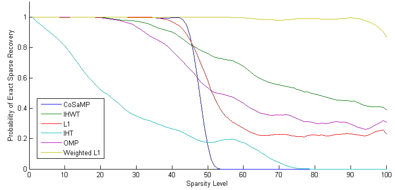
In Figure 1 we present the performance of IHWT, CoSaMP [12], IHT [10], OMP [15], minimization and weighted minimization for the task of exact sparse recovery using measurements. In particular we randomly generated Gaussian sensing matrices, -sparse power law signals and we have the noise-free measurements . We consider a signal to be exactly recovered if the signal approximation and the true underlying signal agree to four decimal places, i.e. . We averaged over 200 trials. Observe that while IHWT does not exactly recover the sparser power law signals as well as CoSaMP or minimization, its recovery performance degrades much more gracefully as the sparsity level increases.
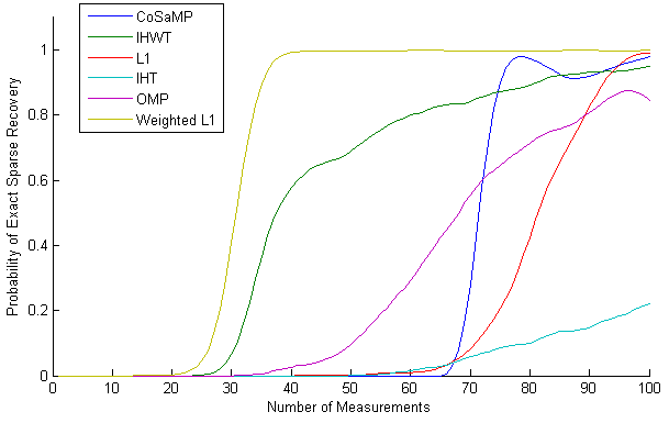
In Figure 2 we now keep the sparsity level fixed at and we allow the number of measurements to vary from 1 to 100. We averaged over 200 runs and we present the probability of exact recovery. Observe the superior performance of IHWT over the other classical greedy sparse approximation algorithms in the undersampling regime.
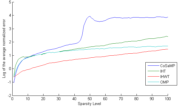
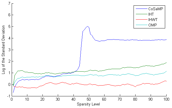
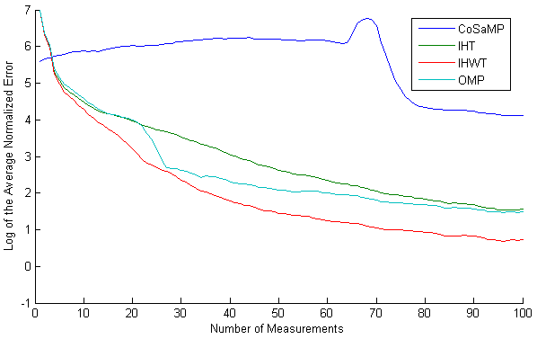
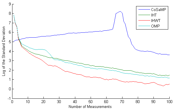
In the next set of experiments, we tested the noisy sparse recovery performance of IHWT and we compared it again three standard sparse approximation algorithms: CoSaMP, IHT and OMP. We have a fixed number of measurements and we randomly generated Gaussian sensing matrices and we have noisy samples . Note now that is no longer an -sparse power law distributed signal but rather it is a dense power law distributed signal. In Figure 3 we present the normalized error and log of the standard deviation averaged over 200 trials and in 4 we present the of the standard deviation of the 200 trials. In Figures 3 and 4 we see the clear performance advantage of IHWT over other greedy algorithms for the task of fixed sparse approximation of power law distributed signals using a fixed number of measurements.
In our final set of experiments, we tested how well we could approximate the best sparse approximation of a dense power law signal given a set of noisy measurements using a variable number of measurements . In Figures 5 and 6 we again see the improved performance of IHWT over other standard greedy sparse approximation algorithms.
5 Conclusion and Future Directions
We have presented the IHWT algorithm which is a weighted extension of the IHT algorithm using the weighted sparsity technology developed in [5]. We established theoretical guarantees of IHWT which are weighted analogues of their unweighted counterparts. While not all of the guarantees presented in [10, 13, 16] are able to be extended, in certain cases like Prop 3.5 and Theorem 3.6 we were able to extend the results using the additional hypothesis that the weight parameter satisfies for a given weighted sparsity . This condition allowed us to control the tail and instead of obtaining error bounds, we obtained the analogous error bounds in the weighted norms. Empirically to test the performance of IHWT, we implemented a tractable surrogate for the projection onto the space of weighted signals. The numerical experiments also show that the normalized version of IHWT has superior performance to their unnormalized counterparts.
We pose the following open problems:
-
1.
Can the results from [13], which guarantee the convergence of IHT to a local minimizer be extended to IHWT? Here we only extended the guarantee that the IHWT sequence of iterates is a contractive sequence.
-
2.
Can we learn the weight parameter given some training data where each is a known signal?
-
3.
Here we simply used the weights from the weighted minimization problem to be our sparsity weights. However, is there a more optimal choice of weights to reduce the performance gap between IHWT and weighted minimization for the task of exact sparse recovery?
Acknowledgements
The author gratefully acknowledges support from Rachel Ward’s Air Force Young Investigator Award and overall guidance from Rachel Ward throughout the entire process.
References
- [1] S. Foucart and H. Rauhut, A Mathematical Introduction to Compressive Sensing. Birkhäuser Mathematics, 2013.
- [2] D. Tolhurst, Y. Tadmor, and T. Chao, “Amplitude spectra of natural images,” Ophthalmic and Physiological Optics, vol. 12, pp. 229–232, April 1992.
- [3] D. Ruderman and W. Bialek, “Statistics of natural images: Scaling in the woods,” Phys. Rev. Lett., vol. 73, no. 6, 1994.
- [4] N. Silver, The Signal and the Noise: Why So Many Predictions Fail but Some Don’t. Penguin Press.
- [5] H. Rauhut and R. Ward, “Interpolation via weighted minimization,” arXiv:1308.0759, August 2013.
- [6] M. Khajehnejad, W. Xu, A. Avestimehr, and B. Hassibi, “Analyzing weighted minimization for sparse recovery with nonuniform sparse models,” IEEE Transactions on Signal Processing, vol. 59, no. 5, pp. 1985–2001, 2011.
- [7] A. Krishnaswamy, S. Oymak, and B. Hassibi, “A simpler approach to weighted minimization,” ICASSP 2012, pp. 3621–3624.
- [8] S. Misra and P. Parrilo, “Analysis of weighted -minimization for model based compressed sensing,” arXiv:1301.1327 [cs.IT], 2013.
- [9] S. Schwartz and A. Tewari, “Stochastic methods for regularized loss minimization,” Journal of Machine Learning Research, vol. 12, pp. 1865–1892, June 2011.
- [10] T. Blumensath and M. Davies, “Iterative hard thresholding for compressed sensing,” Applied and Computational Harmonic Analysis, vol. 27, pp. 265–274, November 2009.
- [11] “Mathematica version 8.0,” 2010.
- [12] D. Needell and J. Tropp, “Cosamp: Iterative signal recovery from incomplete and inaccurate samples,” Applied and Computational Harmonic Analysis, vol. 26, pp. 301–321, May 2009.
- [13] T. Blumensath and M. Davies, “Iterative thresholding for sparse approximations,” Journal of Fourier Analysis and Applications, vol. 14, pp. 629–654, December 2008.
- [14] K. Lange, Optimization. Springer Verlag, 2004.
- [15] J. Tropp and A. Gilbert, “Signal recovery from random measurements via orthogonal matching pursuit,” IEEE Transactions on Information Theory, vol. 53, no. 12, pp. 4655 – 4666, 2007.
- [16] T. Blumensath and M. Davies, “Normalized iterative hard thresholding: Guaranteed stability and performance,” IEEE Journal of Selected Topics in Signal Processing, vol. 4, pp. 298–309, April 2010.