Measuring the Coronal Properties of IC 4329A with NuSTAR

Abstract

We present an analysis of a $\sim 160{\rm\thinspace ks}$ NuSTAR observation of the nearby bright Seyfert galaxy IC 4329A. The high-quality broadband spectrum enables us to separate the effects of distant reflection from the direct coronal continuum, and to therefore accurately measure the high-energy cutoff to be $E_{\rm cut}=178^{+74}_{-40}{\rm\thinspace keV}$. The coronal emission arises from accretion disk photons Compton up-scattered by a thermal plasma, with the spectral index and cutoff being due to a combination of the finite plasma temperature and optical depth. Applying standard Comptonization models, we measure both physical properties independently using the best signal-to-noise obtained to date in an AGN over the $3-79{\rm\thinspace keV}$ band. We derive $kT_{\rm e}=37^{+7}_{-6}{\rm\thinspace keV}$ with $\tau=1.25^{+0.20}_{-0.10}$ assuming a slab geometry for the plasma, and $kT_{\rm e}=33^{+6}_{-6}{\rm\thinspace keV}$ with $\tau=3.41^{+0.58}_{-0.38}$ for a spherical geometry, with both having an equivalent goodness-of-fit.

1 Introduction

The primary hard X-ray continuum in Seyfert galaxies arises from repeated Compton up-scattering of UV/soft X-ray accretion disk photons in a hot, trans-relativistic plasma. This process results in a power-law spectrum extending to energies determined by the electron temperature in the hot “corona” (for a detailed discussion, see Rybicki & Lightman 1979). The power-law index is a function of the plasma temperature, $T$, and optical depth, $\tau$. This scenario describes the hard X-ray/soft $\gamma$-ray spectra of bright Seyferts reasonably well (see, e.g., Zdziarski et al. 2000).

There are few physical constraints on the nature of the corona. Broad-band UV/X-ray spectra require that it not fully cover the disk, and suggest it is probably patchy (Haardt et al. 1994). X-ray microlensing experiments suggest it is compact; in some bright quasars a half-light radius of $r_{\rm c}\leq 6\,r_{\rm g}$ has been measured (Chartas et al. 2009; Reis & Miller 2013), where we define $r_{\rm c}$ as the radius of the corona and $r_{\rm g}\equiv GM/c^{2}$. Eclipses of the X-ray source have also placed constraints on the size of the hard X-ray emitting region(s): $r_{\rm c}\leq 170\,r_{\rm g}$ (e.g., Risaliti 2007; Maiolino et al. 2010; Brenneman et al. 2013).

However, the coronal temperature and optical depth remain poorly constrained due to the lack of high-quality X-ray measurements extending above $10{\rm\thinspace keV}$. Complex spectral components, including reflection from the accretion disk as well as from distant matter, contribute to the $\sim{\rm few}-30{\rm\thinspace keV}$ spectrum, and constraints from previous observations suggest typical cutoff energies are $E_{\rm cut}\geq 150{\rm\thinspace keV}$, requiring spectra extending above $50{\rm\thinspace keV}$ for good constraints. The NuSTAR high energy focusing X-ray telescope (Harrison et al. 2013), which covers the band from $3-79{\rm\thinspace keV}$ with unprecedented sensitivity, provides the capability to measure both the Compton reflection component from neutral material and to constrain the continuum cutoffs in bright systems.

The nearby Seyfert galaxy IC 4329A ($z=0.0161$, Willmer et al. 1991; Galactic $N_{\rm H}=4.61\times 10^{20}\hbox{${\rm\thinspace cm}^{-2}\,$}$, Kalberla et al. 2005; $M_{\rm BH}=1.20\times 10^{8}\hbox{$\rm\thinspace M_{\odot}$}$, de La Calle Pérez et al. 2010) is a good candidate for such measurements. With a $2-10{\rm\thinspace keV}$ flux range of $F_{\rm 2-10}\sim(0.1-1.8)\times 10^{-10}\hbox{${\rm\thinspace erg}{\rm\thinspace cm}^{-2}{\rm\thinspace s}^{-1}\,$}$ (Beckmann et al. 2006; Verrecchia et al. 2007), IC 4329A is one of the brightest Seyferts. In the hard X-ray/soft $\gamma$-ray band it appears similar to an average radio-quiet Seyfert (e.g., Zdziarski et al. 1996). A Compton reflection component and strong Fe K$\alpha$ line (Piro et al. 1990) are both present.

IC 4329A has been observed in the hard X-ray band by BeppoSAX (Perola et al. 2002), ASCA+RXTE (Done et al. 2000) and INTEGRAL (Molina et al. 2013), which placed rough constraints on the high-energy coronal cutoff at $E_{\rm cut}\geq 180{\rm\thinspace keV}$, $E_{\rm cut}=150-390{\rm\thinspace keV}$ and $E_{\rm cut}=60-300{\rm\thinspace keV}$, respectively. Combining INTEGRAL and XMM-Newton data further constrained the cutoff energy to $E_{\rm cut}=152^{+51}_{-32}{\rm\thinspace keV}$ (Molina et al. 2009). The soft X-ray spectrum is absorbed by a combination of neutral and partially ionized gas, with a total column of $\sim 3\times 10^{21}\hbox{${\rm\thinspace cm}^{-2}\,$}$ (Zdziarski 1994; Madejski et al. 1995; Steenbrugge et al. 2005), comparable to the host galaxy’s ISM column density (Wilson & Penston 1979). After accounting for the reflection component, the intrinsic spectral variability is modest (Madejski et al. 2001; Miyazawa et al. 2009; Markowitz 2009).

We report here on the NuSTAR portion of our simultaneous NuSTAR+Suzaku observation of IC 4329A. The combined NuSTAR+Suzaku analysis will be described in a forthcoming paper (Brenneman et al. , in prep.). In §2, we report on the NuSTAR observations. Our spectral analysis follows in §3, with a discussion of the coronal properties and their implications in §4.

2 Observations and Data Reduction

IC 4329A was observed by NuSTAR quasi-continuously from August 12-16, 2012. After eliminating Earth occultations, passages through the South Atlantic Anomaly (SAA) and other periods of high background, the NuSTAR observation totaled $\sim 162{\rm\thinspace ks}$ of on-source time for focal plane module A (FPMA) and $159{\rm\thinspace ks}$ for FPMB. The total counts after background subtraction in the $3-79{\rm\thinspace keV}$ band were $426,274$ and $403,588$ for each instrument, yielding signal-to-noise (S/N) ratios of $26.8$ and $24.6$, respectively.

The NuSTAR data were collected with the FPMA and FPMB optical axes placed roughly $\sim 2$ arcmin from the nucleus of IC 4329A. We reduced the data using the NuSTAR Data Analysis Software (nustardas) and calibration version 1.1.1. We filtered the event files and applied the default depth correction using the nupipeline task. We used circular extraction regions $75$ arcsec in radius for the source and background, with the source region centered on IC 4329A and the background taken from the corner of the same detector, as close as possible to the source without being contaminated by the PSF wings. Spectra, images and light curves were extracted and response files were generated using the nuproducts task. In order to minimize systematic effects, we have not combined responses or spectra from FPMA and FPMB, but instead fit them simultaneously. We allow the absolute normalization for both modules to vary, and we find a cross-calibration factor of $1.072\pm 0.002$ for FPMB relative to FPMA.

For all the analysis we used xspec version 12.8.1, along with other ftools packages within HEASoft 6.14. All errors in the text are 1$\sigma$ confidence within the text unless otherwise specified, while the final parameter values and their uncertainties are quoted in Table 1 at $90\%$ confidence.

IC 4329A demonstrated a modest, secular flux evolution during our observation, increasing by $\sim 12\%$ over the first $50{\rm\thinspace ks}$ of the observation (using clock time), plateauing at maximum flux for $\sim 50{\rm\thinspace ks}$ then decreasing by $\sim 34\%$ over the remainder of the observation. On average, the flux we measure, $1.02\times 10^{-10}\hbox{${\rm\thinspace erg}{\rm\thinspace cm}^{-2}{\rm\thinspace s}^{-1}\,$}$, is within its historical range of values. Given the lack of short term variability and modest flux evolution we use the time-averaged spectrum for all spectral analysis (§3).

3 Spectral Analysis

The focus of this paper is the characterization of the primary high-energy continuum in IC 4329A, and we therefore restrict our analysis to $5-79{\rm\thinspace keV}$ to avoid the effects of low-energy absorption which are poorly constrained by NuSTAR alone. We assess the contributions of distant reflection from the outer disk and/or torus, although we defer a detailed discussion of the distant and inner disk reflection to a forthcoming paper (Brenneman et al. , in prep.).

3.1 Phenomenological Modeling of the NuSTAR Spectra

We first consider a phenomenological model for the NuSTAR spectra to generally investigate the prominence of the high-energy cutoff. We begin by evaluating the $5-79{\rm\thinspace keV}$ data against the pexmon model (Nandra et al. 2007), which incorporates both primary emission (in the form of a power-law with an exponential cutoff) and distant reflection. Pexmon is based on the pexrav model of Zdziarski et al. (1995), but in addition to the reprocessed continuum emission it also includes the fluorescent emission lines expected to accompany the Compton reflection (Fe K$\alpha$, Fe K$\beta$, Ni K$\alpha$ and the Fe K$\alpha$ Compton shoulder).

Fitting the $5-79{\rm\thinspace keV}$ data using pexmon with no exponential cutoff or reflection ($E_{\rm cut}=10^{6}{\rm\thinspace keV}$ and $R=0$) yields a goodness-of-fit of $\chi^{2}/\nu=2704/1723\,(1.57)$, with clear residuals remaining in the Fe K band (Fig. 1, top). The power-law has a slope of $\Gamma=1.71\pm 0.01$. The spectrum has a pronounced convex shape characteristic of both Compton reflection and a high-energy cutoff above $\sim 30{\rm\thinspace keV}$.

Allowing the reflection component to fit freely, we get $R=-0.42\pm 0.02$ (negative because of the way reflection is parameterized within the model; the absolute value is the real reflection fraction) with $\Gamma=1.83\pm 0.02$, for $\chi^{2}/\nu=2010/1722\,(1.17)$. Clear residual curvature above $\sim 25{\rm\thinspace keV}$ remains (Fig. 1, middle). Also freeing the cutoff energy of the primary continuum yields $E_{\rm cut}=149\pm 16{\rm\thinspace keV}$ with $\Gamma=1.70\pm 0.02$ and $R=-0.34\pm 0.03$ with $\chi^{2}/\nu=1881/1721\,(1.09)$ (Fig. 1, bottom). It is clear that both Compton reflection and a high-energy cutoff are required: the improvement in fit of $\Delta\chi^{2}/\Delta\nu=-129/-1$ ($\sim 7\%$) upon addition of a high-energy cutoff is highly significant.

Freeing the iron abundance (while keeping the abundances of other elements fixed to their solar values) improves the fit only slightly to $\chi^{2}/\nu=1871/1720\,(1.09)$, with Fe/solar$=1.57\pm 0.22$, though the uncertainties on the other parameters increase slightly as a result. Allowing the inclination angle of the reflector to fit freely yields no constraints on the parameter and no further improvement in fit, so we have elected to keep it fixed at $i=60^{\circ}$. We note that when the pexmon component is replaced with the more common model of pexrav plus Gaussian emission lines, the fit yields similar values of $\Gamma$, $R$ and $E_{\rm cut}$.

Residuals still remain in the Fe K band, suggesting the presence of an underlying broad component of the Fe K$\alpha$ line. When this feature is modeled with a Gaussian ($E=6.51\pm 0.05{\rm\thinspace keV}$, $\sigma=0.36\pm 0.03{\rm\thinspace keV}$, $EW=60\pm 15{\rm\thinspace eV}$), the goodness-of-fit improves to $\chi^{2}/\nu=1831/1717\,(1.07)$. Including this component also lowers the iron abundance to Fe/solar$=0.87\pm 0.21$. We refer to this model hereafter as Model 1. The modest broad iron line detection will be discussed at length in Brenneman et al. (in prep.), and will not be further addressed in this work.

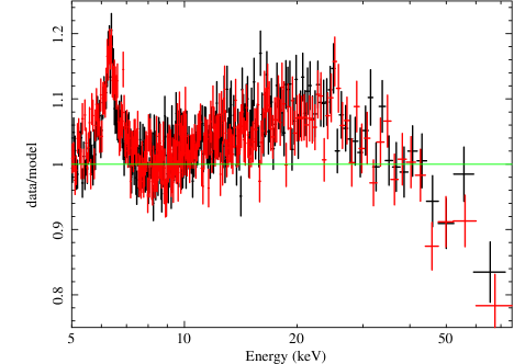
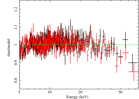
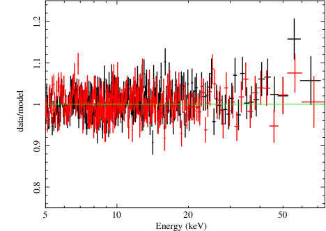
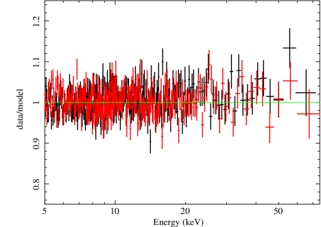
Figure 1: Plots of the data-to-model ratio of the NuSTAR/FPMA (black) and FPMB (red) spectra vs. a pexmon model without an exponential cutoff or reflection (top left), including reflection (top right), including an exponential cutoff in addition to reflection (bottom left), and including also a broad Gaussian Fe K$\alpha$ line (bottom right). The horizontal green line in each plot represents a perfect fit.

3.2 Toward a More Physical Model

The high S/N of the data enable us to consider more physically motivated models to describe the continuum emission. We employ the compPS model of Poutanen & Svensson (1996), which produces the continuum through inverse Compton scattering of thermal disk photons off of relativistic electrons situated above the disk in a choice of geometries. The disk photons and coronal plasma are each parametrized by a single temperature. It then reflects the continuum X-rays off of a slab of gas (the disk or torus) to produce reprocessed continuum emission self-consistently by internally linking with the pexrav model. Reprocessed line emission is not included.

We fix the energy of the thermal disk photons to $kT_{\rm disk}=30{\rm\thinspace eV}$, appropriate for a black hole of $M_{\rm BH}\approx 10^{8}\hbox{$\rm\thinspace M_{\odot}$}$ (Frank et al. 2002). We initially fix the geometry of the hot electrons to be spherical with a Maxwellian distribution, the former choice being based on the coronal compactness measurements cited in §1 (e.g., Chartas et al. 2009), although we also compare the results with a slab geometry. We fit for the electron energy ($kT_{\rm e}$) and coronal optical depth ($\tau$), as well as for the reflection fraction ($R$) of the reprocessing gas, and model normalization ($K$). We add in separate Gaussian components to represent the Fe K$\alpha$ (narrow and broad) and K$\beta$ line emission resulting from reflection in order to maintain consistency with the pexmon model employed in §3.1 above.

This approach yields approximately the same global goodness-of-fit as Model 1: $\chi^{2}/\nu=1849/1715\,(1.07)$, with parameter values of $kT_{\rm e}=48\pm 22{\rm\thinspace keV}$ (assuming that $E_{\rm cut}=3kT_{\rm e}$, as per Petrucci et al. 2001, this is equivalent to a cutoff energy of approximately $144\pm 66{\rm\thinspace keV}$, consistent with that measured in Model 1), $\tau=2.70\pm 1.31$ and $R=-0.39\pm 0.06$, assuming a distant, neutral reflector inclined at $60^{\circ}$ to the line of sight. We note that the iron abundance is not constrained by the model. The narrow Gaussian components representing narrow Fe K$\alpha$ and K$\beta$ have equivalent widths of $EW_{\rm K\alpha}=41\pm 8{\rm\thinspace eV}$ and $EW_{\rm K\beta}=15\pm 12{\rm\thinspace eV}$, respectively. The addition of these components improves the global goodness-of-fit by $\Delta\chi^{2}=483$ and $\Delta\chi^{2}=19$, respectively, each for three additional degrees of freedom.

We also note that consistent results are achieved (within errors) when we fit for the Compton-y parameter rather than the optical depth, as per the approach taken in Petrucci et al. (2013): $kT_{\rm e}=43\pm 41{\rm\thinspace keV}$ and $y=1.16\pm 0.05$, resulting in $\tau=3.45\pm 0.95$. In addition to having larger parameter uncertainties, however, this approach also results in an unconstrained reflection fraction. Consistent results are obtained when we fix the reflection fraction at $R=-0.39$ (as described in the previous paragraph) and Fe/solar$=1$: $kT_{\rm e}=39\pm 9{\rm\thinspace keV}$, $y=1.06\pm 0.01$ and $\tau=3.47\pm 0.25$. However, in light of the importance of probing the reflection as a free parameter, we have elected to fit for the optical depth explicitly in the model.

We consider a slab geometry for the corona as well, again with a Maxwellian electron distribution. This results in no significant improvement to the fit: $\chi^{2}/\nu=1836/1713\,(1.07)$, with $kT_{\rm e}=48\pm 13{\rm\thinspace keV}$ (equivalent to a cutoff energy of $E_{\rm cut}=144\pm 39{\rm\thinspace keV}$, also consistent with that‘ measured in Model 1), $\tau=1.50\pm 0.39$ and $R=-0.38\pm 0.07$. This model is also insensitive to the Fe abundance. The equivalent widths of the Gaussian lines are the same as for the spherical geometry, within errors.

For both geometries the electron plasma temperature is constant within errors, while the optical depth is pushing the upper limit of its sensible parameter space. We therefore check the compPS results using the compTT model (Titarchuk 1994), which assumes a simpler thermal electron distribution and does not self-consistently include the Compton reflection continuum. We add in reflection from distant matter using the pexmon model. We assume an incident power-law photon index of $\Gamma=1.70$ (fixed), as found in Model 1, and tie the normalization of the reflected emission to that of the Comptonized component, such that the contribution of the reflector relative to the Comptonization is entirely determined by $R$ and the iron abundance. We checked the models to ensure a tight match between the shapes of a power-law of this index and the shape of the compTT component. We also fix the cutoff energy of the incident power-law at $E_{\rm cut}=3kT_{\rm e}$. The spherical geometry compTT component model and the same model with a slab geometry are referred to hereafter as Models 2-3, respectively.

We find values for the coronal temperature consistent within errors with those of compPS for both the spherical and slab geometries: $kT_{\rm e}=33\pm 11{\rm\thinspace keV}$ and $kT_{\rm e}=37\pm 16{\rm\thinspace keV}$, respectively. The coronal optical depth in the slab geometry is slightly smaller with compTT vs. compPS, though consistent within errors: $\tau=1.25\pm 0.50$. For the spherical geometry, $\tau=3.41\pm 0.90$, also consistent with its compPS analog within errors. The reflection fraction measured with this model (defined in the same way for both geometries) is comparable to that determined by compPS: $R=-0.33\pm 0.03$ for the sphere and $R=-0.32\pm 0.04$ for the slab. The iron abundance is comparable that that found in Model 1: Fe/solar$=0.63\pm 0.20$ (sphere) and Fe/solar$=0.68\pm 0.20$ (slab).

Table 1 provides the best-fit parameters and their Markov Chain Monte Carlo (MCMC)-derived $90\%$ confidence errors for all three models. Fig. 2 plots the contributions of individual model components to the overall fit. We show only the components for Model 1, since Models 2-3 look virtually identical, except using a Comptonization component in lieu of a power-law. The total absorbed $5-79{\rm\thinspace keV}$ flux and luminosity are $F_{5-79}=3.04\times 10^{-10}\hbox{${\rm\thinspace erg}{\rm\thinspace cm}^{-2}{\rm\thinspace s}^{-1}\,$}$ and $L_{5-79}=1.77\times 10^{44}\hbox{${\rm\thinspace erg}{\rm\thinspace s}^{-1}\,$}$, respectively.

The MCMC analysis employed to determine the formal parameter distribution used the Metropolis-Hastings algorithm (e.g., Kashyap & Drake 1998 and references therein) following the basic procedures outlined in, e.g., Reynolds et al. (2012). Using this basic procedure we generated probability density contours for the most interesting pairs of parameters for each model, shown in Figs. 3-4. Both sets of contours are closed, implying that $kT_{\rm e}$ and $\tau$ are independently constrained to $99\%$ confidence in both the spherical and slab geometries. Nonetheless, some degeneracy between the two parameters still remains, as evidenced by the linear correlation seen in each plot, due to an inherent modeling degeneracy between the optical depth and temperature of the electron plasma in each geometry. Fig. 4 depicts the modest range over which these parameters are degenerate, which is $\pm 18\%$ of the parameter space in temperature and ${}^{+17\%}_{-11\%}$ in optical depth for the sphere, versus ${}^{+19\%}_{-16\%}$ in temperature and ${}^{+16\%}_{-8\%}$ in optical depth for the slab.

Component	Parameter (units)	Model 1	Model 2	Model 3
TBabs	$N_{\rm H}\,(\times 10^{20}\hbox{${\rm\thinspace cm}^{-2}\,$})$	$4.61(f)$	$4.61(f)$	$4.61(f)$
pexmon	$\Gamma$	$1.70^{+0.04}_{-0.04}$	$1.70(f)$	$1.70(f)$
	$E_{\rm cut}\,({\rm\thinspace keV})$	$178^{+74}_{-40}$	$90^{+51}_{-18}*$	$96^{+63}_{-24}*$
	$K_{\rm pex}\,(\times 10^{-2}\hbox{${\rm\thinspace ph}{\rm\thinspace cm}^{-2}{\rm\thinspace s}^{-1}\,$})$	$2.90^{+0.20}_{-0.18}$	$2.90(f)$	$2.90(f)$
	$R$	$-0.29^{+0.06}_{-0.06}$	$-0.33^{+0.04}_{-0.04}$	$-0.32^{+0.04}_{-0.04}$
	Fe/solar	$0.87^{+0.42}_{-0.31}$	$0.63^{+0.20}_{-0.20}$	$0.68^{+0.21}_{-0.19}$
compTT	$kT_{\rm e}\,({\rm\thinspace keV})$	$---$	$33^{+6}_{-6}*$	$37^{+7}_{-6}*$
	$\tau$	$---$	$3.41^{+0.58}_{-0.38}$	$1.25^{+0.20}_{-0.10}$
	$K_{\rm com}\,(\times 10^{-3}\hbox{${\rm\thinspace ph}{\rm\thinspace cm}^{-2}{\rm\thinspace s}^{-1}\,$})$	$---$	$9.01^{+1.88}_{-2.95}$	$8.17^{+2.37}_{-2.96}$
zgauss	$E_{\rm b}\,({\rm\thinspace keV})$	$6.51^{+0.05}_{-0.05}$	$6.49^{+0.07}_{-0.06}$	$6.48^{+0.08}_{-0.06}$
	$\sigma_{\rm b}\,({\rm\thinspace keV})$	$0.36^{+0.12}_{-0.10}$	$0.36^{+0.09}_{-0.08}$	$0.37^{+0.10}_{-0.08}$
	$K_{\rm b}\,(\times 10^{-5}\hbox{${\rm\thinspace ph}{\rm\thinspace cm}^{-2}{\rm\thinspace s}^{-1}\,$})$	$7.84^{+2.72}_{-2.61}$	$9.09^{+2.59}_{-2.50}$	$9.11^{+2.64}_{-2.54}$
	$EW_{\rm b}\,({\rm\thinspace eV})$	$60^{+21}_{-20}$	$70^{+20}_{-19}$	$70^{+20}_{-20}$
Final fit		$1831/1717\,(1.07)$	$1836/1718\,(1.07)$	$1837/1718\,(1.07)$

Table 1: Best-fit parameters, their values and errors (to $90\%$ confidence) for Models 1-3. Parameters marked with an (f) are held fixed in the fit, while those marked with an (*) are tied to another parameter.

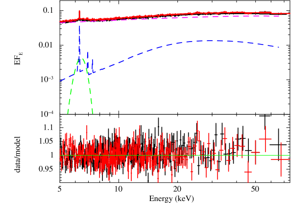
Figure 2: Upper panel: $EF_{\rm E}$ vs. energy plot for Model 1 vs. the FPMA (black points) and FPMB (red points) data. The pexmon model incorporating the cutoff power-law continuum and distant reflection is in dashed red, the direct power-law emission is in dashed blue, and the broad Gaussian in dashed green. The summed models are in solid black (FPMA) and solid red (FPMB). Lower panel: Data-to-model ratio for the FPMA (black) and FPMB (red). The horizontal green line shows a ratio of unity for reference.

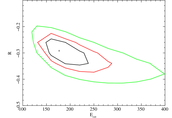
Figure 3: Output from the MCMC analysis of Model 1: contours show the $67\%$ (black), $90\%$ (red) and $99\%$ (green) probability densities for $R$ vs. $E_{\rm cut}$.

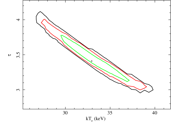
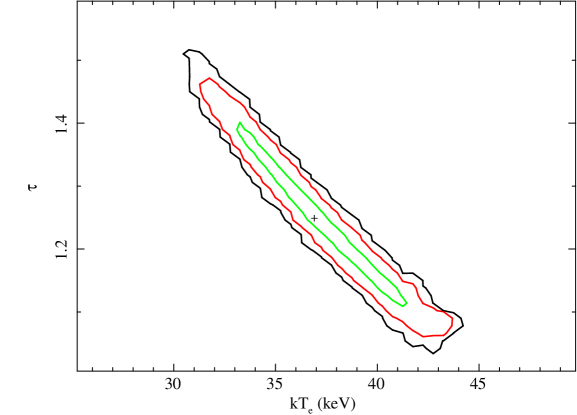
Figure 4: Output from the MCMC analysis of Model 2 (sphere; upper panel) and Model 3 (slab; lower panel): contours show the $67\%$ (green), $90\%$ (red) and $99\%$ (black) probability densities for $\tau$ vs. $kT_{\rm e}$.

4 Discussion

The time-averaged $5-79{\rm\thinspace keV}$ NuSTAR spectrum is well-described by a largely phenomenological pexmon model (Model 1) that includes, to $90\%$ confidence, a continuum power-law with $\Gamma=1.70\pm 0.03$, and a high energy cutoff of $E_{\rm cut}=178^{+74}_{-40}{\rm\thinspace keV}$, as well as reprocessed emission from a distant reflector ($R=-0.29^{+0.06}_{-0.06}$, Fe/solar$=0.87^{+0.42}_{-0.31}$). Prior measurements provided constraints on the cutoff energy of the power-law at $E_{\rm cut}\geq 180{\rm\thinspace keV}$ (Perola et al. 2002), $E_{\rm cut}=150-390{\rm\thinspace keV}$ (Done et al. 2000) and $E_{\rm cut}=60-300{\rm\thinspace keV}$ (Molina et al. 2013), though Molina et al. (2009) did achieve a more precise constraint of $E_{\rm cut}=152^{+51}_{-32}{\rm\thinspace keV}$ using XMM in tandem with INTEGRAL. The two datasets were not taken simultaneously, however, and the S/N achieved by the NuSTAR data is superior to that of INTEGRAL. We therefore consider our new measurements —which agree with all of the previously mentioned values, within errors— to be more robust.

The high-S/N, simultaneously obtained broad band NuSTAR spectrum enables us to apply physical models for the underlying coronal continuum emission that go beyond phenomenological descriptions. The models parametrize the temperature, and optical depth of the electron plasma for two coronal geometries; a sphere and a slab. Both geometries fit the data equally well, though we note that the sphere model provides tighter constraints on its parameters. Both models also produce consistent values for the electron temperature within errors. However, they result in slightly different values for the optical depth: $kT_{\rm e}=37^{+7}_{-6}{\rm\thinspace keV}$ with $\tau=1.25^{+0.20}_{-0.10}$ for the slab geometry, compared with $kT_{\rm e}=33^{+6}_{-6}{\rm\thinspace keV}$ with $\tau=3.41^{+0.58}_{-0.38}$ for the spherical geometry (both at $90\%$ confidence).

This discrepancy in optical depth is due primarily to the way that the value is calculated for a given geometry within the Comptonization models we employ (e.g., Titarchuk 1994; Poutanen & Svensson 1996): the optical depth for a slab geometry is taken vertically, whereas that for a sphere is taken radially and thus incorporates an extra factor of $1/{\rm cos}(60)=2$. Taking this extra factor into account, the optical depth of the spherical case can be translated into the slab geometry for ease of comparison: $\tau=1.71^{+0.29}_{-0.19}$ for the sphere vs. $\tau=1.25^{+0.20}_{-0.10}$ for the slab. Though these values do not formally agree within their $90\%$ confidence errors, they are compatible at the $2\sigma$ level.

The derived electron temperatures for the sphere and slab coronal geometries are low compared to $E_{\rm cut}/2$, but are not far off from $E_{\rm cut}/3$, which is consistent with the corona having significant optical depth (i.e., $\tau>1$), modulo uncertainties in geometry, seed photons, outflows, anisotropy, etc. which we are not able to probe even with our high-S/N data. Due to an inherent modeling degeneracy between the optical depth and temperature of the electron plasma in each geometry, there is a small, linearly correlated range of values for these parameters which demonstrate approximately equal statistical fit quality, as can be seen in Figs. 3-4. Nonetheless, we constrain both parameters precisely and accurately with the best data ever achieved over this energy band. The data quality and goodness-of-fit of the Comptonization models gives us confidence in the temperatures and optical depths we have measured. We note, however, that without high-S/N data at energies $\geq 100{\rm\thinspace keV}$ we are unable to discriminate between a thermal and non-thermal population of coronal electrons (e.g., with a model such as eqpair, Coppi 1999). A significant non-thermal contribution could change the temperatures and optical depths that we measure.

With our robust determination of the continuum shape over the broad energy range, we estimate that the power dissipated in the corona, in the form of the power-law continuum, is $\sim 87\%$ of the total luminosity of the entire system from $5-79{\rm\thinspace keV}$ (the power-law has a luminosity of $L_{5-79}=1.53\times 10^{44}\hbox{${\rm\thinspace erg}{\rm\thinspace s}^{-1}\,$}$). This represents $\sim 10\%$ of the bolometric luminosity of the source ($L_{\rm bol}=1.60\times 10^{45}\hbox{${\rm\thinspace erg}{\rm\thinspace s}^{-1}\,$}$; de La Calle Pérez et al. 2010). Given that IC 4329A is a radio-quiet AGN (total 10 MHz - 100 GHz $L_{\rm r}=2.2\times 10^{39}\hbox{${\rm\thinspace erg}{\rm\thinspace s}^{-1}\,$}$; Wilson & Ulvestad 1982), we do not expect a significant portion of the X-rays to come from a jet component, so we may infer that the remaining $\sim 13\%$ of the $5-79{\rm\thinspace keV}$ emission represents the contribution from reflection.

Our spectral fitting results are broadly consistent with the signatures expected from dynamic, outflowing coronae as defined by Beloborodov (1999) and Malzac et al. (2001): a hard spectral index and relatively weak reflection. If the corona is really powered by compact magnetic flares that are dominated by $e^{\pm}$ pairs, the resulting plasma is subject to radiation pressure from the photons moving outwards from the disk. The bulk velocity at which the plasma should be outflowing from the disk, given our Model 1 photon index of $\Gamma=1.70$, is $v=0.22c$, according to Beloborodov (1999). Our measured reflection fraction of $R=0.3$ is also consistent with that predicted by Malzac et al. (2001) for a Comptonizing plasma with these parameters. We note that the beaming of the coronal emission inherent in such dynamic models not only hardens the spectrum, but also implies that the intrinsic break in the spectrum occurs at lower energies than what is observed: i.e., $E_{\rm cut}\sim 100{\rm\thinspace keV}$ rather than $E_{\rm cut}=178^{+74}_{-40}{\rm\thinspace keV}$, as measured with Model 1. A lower intrinsic rollover is consistent with our measurements of the electron temperature from Comptonization models ($kT\sim 35{\rm\thinspace keV}$), if we assume that $E_{\rm cut}$ is between $2-3\,kT_{\rm e}$.

References

- Beckmann et al. (2006) Beckmann, V., Gehrels, N., Shrader, C. R., & Soldi, S. 2006, ApJ, 638, 642
- Beloborodov (1999) Beloborodov, A. M. 1999, ApJ, 510, L123
- Brenneman et al. (2013) Brenneman, L. W., Risaliti, G., Elvis, M., & Nardini, E. 2013, MNRAS, 429, 2662
- Chartas et al. (2009) Chartas, G., Kochanek, C. S., Dai, X., Poindexter, S., & Garmire, G. 2009, ApJ, 693, 174
- Coppi (1999) Coppi, P. S. 1999, in Astronomical Society of the Pacific Conference Series, Vol. 161, High Energy Processes in Accreting Black Holes, ed. J. Poutanen & R. Svensson, 375
- de La Calle Pérez et al. (2010) de La Calle Pérez, I., Longinotti, A. L., Guainazzi, M., Bianchi, S., Dovčiak, M., Cappi, M., Matt, G., Miniutti, G., Petrucci, P. O., Piconcelli, E., Ponti, G., Porquet, D., & Santos-Lleó, M. 2010, A&A, 524, A50
- Done et al. (2000) Done, C., Madejski, G. M., & Życki, P. T. 2000, ApJ, 536, 213
- Frank et al. (2002) Frank, J., King, A., & Raine, D. J. 2002, Accretion Power in Astrophysics: Third Edition (Cambridge University Press)
- Haardt et al. (1994) Haardt, F., Maraschi, L., & Ghisellini, G. 1994, ApJ, 432, L95
- Harrison et al. (2013) Harrison, F. A., Craig, W. W., Christensen, F. E., Hailey, C. J., Zhang, W. W., Boggs, S. E., Stern, D., Cook, W. R., Forster, K., Giommi, P., Grefenstette, B. W., Kim, Y., Kitaguchi, T., Koglin, J. E., Madsen, K. K., Mao, P. H., Miyasaka, H., Mori, K., Perri, M., Pivovaroff, M. J., Puccetti, S., Rana, V. R., Westergaard, N. J., Willis, J., Zoglauer, A., An, H., Bachetti, M., Barrière, N. M., Bellm, E. C., Bhalerao, V., Brejnholt, N. F., Fuerst, F., Liebe, C. C., Markwardt, C. B., Nynka, M., Vogel, J. K., Walton, D. J., Wik, D. R., Alexander, D. M., Cominsky, L. R., Hornschemeier, A. E., Hornstrup, A., Kaspi, V. M., Madejski, G. M., Matt, G., Molendi, S., Smith, D. M., Tomsick, J. A., Ajello, M., Ballantyne, D. R., Baloković, M., Barret, D., Bauer, F. E., Blandford, R. D., Brandt, W. N., Brenneman, L. W., Chiang, J., Chakrabarty, D., Chenevez, J., Comastri, A., Dufour, F., Elvis, M., Fabian, A. C., Farrah, D., Fryer, C. L., Gotthelf, E. V., Grindlay, J. E., Helfand, D. J., Krivonos, R., Meier, D. L., Miller, J. M., Natalucci, L., Ogle, P., Ofek, E. O., Ptak, A., Reynolds, S. P., Rigby, J. R., Tagliaferri, G., Thorsett, S. E., Treister, E., & Urry, C. M. 2013, ApJ, 770, 103
- Kalberla et al. (2005) Kalberla, P. M. W., Burton, W. B., Hartmann, D., Arnal, E. M., Bajaja, E., Morras, R., & Pöppel, W. G. L. 2005, A&A, 440, 775
- Kashyap & Drake (1998) Kashyap, V. & Drake, J. J. 1998, ApJ, 503, 450
- Madejski et al. (2001) Madejski, G., Done, C., & Życki, P. 2001, Advances in Space Research, 28, 369
- Madejski et al. (1995) Madejski, G. M., Zdziarski, A. A., Turner, T. J., Done, C., Mushotzky, R. F., Hartman, R. C., Gehrels, N., Connors, A., Fabian, A. C., Nandra, K., Celotti, A., Rees, M. J., Johnson, W. N., Grove, J. E., & Starr, C. H. 1995, ApJ, 438, 672
- Maiolino et al. (2010) Maiolino, R., Risaliti, G., Salvati, M., Pietrini, P., Torricelli-Ciamponi, G., Elvis, M., Fabbiano, G., Braito, V., & Reeves, J. 2010, A&A, 517, A47
- Malzac et al. (2001) Malzac, J., Beloborodov, A. M., & Poutanen, J. 2001, MNRAS, 326, 417
- Markowitz (2009) Markowitz, A. 2009, ApJ, 698, 1740
- Miyazawa et al. (2009) Miyazawa, T., Haba, Y., & Kunieda, H. 2009, PASJ, 61, 1331
- Molina et al. (2013) Molina, M., Bassani, L., Malizia, A., Stephen, J. B., Bird, A. J., Bazzano, A., & Ubertini, P. 2013, MNRAS, 433, 1687
- Molina et al. (2009) Molina, M., Bassani, L., Malizia, A., Stephen, J. B., Bird, A. J., Dean, A. J., Panessa, F., de Rosa, A., & Landi, R. 2009, MNRAS, 399, 1293
- Nandra et al. (2007) Nandra, K., O’Neill, P. M., George, I. M., & Reeves, J. N. 2007, MNRAS, 382, 194
- Perola et al. (2002) Perola, G. C., Matt, G., Cappi, M., Fiore, F., Guainazzi, M., Maraschi, L., Petrucci, P. O., & Piro, L. 2002, A&A, 389, 802
- Petrucci et al. (2001) Petrucci, P. O., Haardt, F., Maraschi, L., Grandi, P., Malzac, J., Matt, G., Nicastro, F., Piro, L., Perola, G. C., & De Rosa, A. 2001, ApJ, 556, 716
- Petrucci et al. (2013) Petrucci, P.-O., Paltani, S., Malzac, J., Kaastra, J. S., Cappi, M., Ponti, G., De Marco, B., Kriss, G. A., Steenbrugge, K. C., Bianchi, S., Branduardi-Raymont, G., Mehdipour, M., Costantini, E., Dadina, M., & Lubiński, P. 2013, A&A, 549, A73
- Piro et al. (1990) Piro, L., Yamauchi, M., & Matsuoka, M. 1990, ApJ, 360, L35
- Poutanen & Svensson (1996) Poutanen, J. & Svensson, R. 1996, ApJ, 470, 249
- Reis & Miller (2013) Reis, R. C. & Miller, J. M. 2013, ApJ, 769, L7
- Reynolds et al. (2012) Reynolds, C. S., Brenneman, L. W., Lohfink, A. M., Trippe, M. L., Miller, J. M., Fabian, A. C., & Nowak, M. A. 2012, ApJ, 755, 88
- Risaliti (2007) Risaliti, G. et al.. 2007, ApJ, 659, L111
- Rybicki & Lightman (1979) Rybicki, G. B. & Lightman, A. P. 1979, Radiative processes in astrophysics (John Wiley & Sons Inc.)
- Steenbrugge et al. (2005) Steenbrugge, K. C., Kaastra, J. S., Sako, M., Branduardi-Raymont, G., Behar, E., Paerels, F. B. S., Blustin, A. J., & Kahn, S. M. 2005, A&A, 432, 453
- Titarchuk (1994) Titarchuk, L. 1994, ApJ, 434, 570
- Verrecchia et al. (2007) Verrecchia, F., in’t Zand, J. J. M., Giommi, P., Santolamazza, P., Granata, S., Schuurmans, J. J., & Antonelli, L. A. 2007, A&A, 472, 705
- Willmer et al. (1991) Willmer, C. N. A., Focardi, P., Chan, R., Pellegrini, P. S., & da Costa, N. L. 1991, AJ, 101, 57
- Wilson & Penston (1979) Wilson, A. S. & Penston, M. V. 1979, ApJ, 232, 389
- Wilson & Ulvestad (1982) Wilson, A. S. & Ulvestad, J. S. 1982, ApJ, 263, 576
- Zdziarski et al. (1995) Zdziarski, A. A., Fabian, A. C., Nandra, K., Celotti, A., Rees, M. J., Done, C., Coppi, P. S., & Madejski, G. M. 1995, ApJ, 438, L63
- Zdziarski et al. (1996) Zdziarski, A. A., Gierlinski, M., Gondek, D., & Magdziarz, P. 1996, A&AS, 120, C553
- Zdziarski et al. (2000) Zdziarski, A. A., Poutanen, J., & Johnson, W. N. 2000, ApJ, 542, 703
- Zdziarski (1994) Zdziarski, A. A. et al.. 1994, MNRAS, 269, L55