$1/f$ noise for intermittent quantum dots exhibits non-stationarity and critical exponents

Abstract

The power spectrum of quantum dot fluorescence exhibits $1/f^{\beta}$ noise, related to the intermittency of these nanosystems. As in other systems exhibiting $1/f$ noise, this power spectrum is not integrable at low frequencies, which appears to imply infinite total power. We report measurements of individual quantum dots that address this long-standing paradox. We find that the level of $1/f^{\beta}$ noise decays with the observation time. The change of the spectrum with time places a bound on the total power. These observations are in stark contrast with most measurements of noise in macroscopic systems which do not exhibit any evidence for non-stationarity. We show that the traditional description of the power spectrum with a single exponent $\beta$ is incomplete and three additional critical exponents characterize the dependence on experimental time.

• August 2014

Keywords: Nanocrystals, Flicker noise, blinking, power spectral density

1 Introduction

The power spectrum of many natural signals exhibits $1/f$ noise at low frequencies [1, 2]. This noise appears in an extremely broad range of systems that includes electrical signals in vacuum tubes, semiconductor devices, and metal films [3, 4], as well as earthquakes [5], network traffic [6], evolution [7], and human cognition [8]. All these systems are characterized by a power spectrum of the universal form $S(f)\sim{A/f^{\beta}}$, where the exponent $\beta$ is between $0$ and $2$ [3, 9, 10]. The long time that has passed from the first discovery of this phenomenon [11] led to multiple theories, competing schools of thought and many unresolved problems. One of the major problems lies in the fact that the spectrum is not integrable at low frequencies if $\beta>1$, i.e., $\int_{0}^{\infty}S(f){\rm d}f=\infty$. This is a paradoxical issue since the total power cannot be infinite, as implied by the divergence of the integral to infinity. In order to solve this paradox, Mandelbrot suggested that $1/f$ noises are related to non-stationary processes [3]. However, $1/f$ noise in macroscopic systems, where a large number of subunits are intrinsically averaged, do not exhibit evidence of non-stationarity [10], hence this famous paradox remains open. Moreover, these ideas have been often contested, for example, by assuming that there exist some low-frequency cutoff $f_{c}$ under which the non-integrable $1/f$ spectrum is no longer observed. For this reason, several groups have increased the measurement time in an attempt to find this evasive low-frequency cutoff. For example, spectral estimations have been obtained for one cycle in three weeks in operational amplifiers [12] and one cycle in 300 years in weather data [13]. Despite such long measurements, no low-frequency cutoff was found in these systems.

During the last two decades, experimental work has shown that $1/f$ noise is also observed in a vast array of nanoscale systems. For example, such noise was observed in individual ion channel conductivity [14, 15], electrochemical signals in nanoscale electrodes [16], biorecognition processes leading to the formation of a complex [17], and graphene devices [18]. Noise in nanoscale systems is particularly intriguing due to their sensitivity to environmental conditions. Furthermore, the characterization of noise properties in nanomaterials is an important challenge with direct applications in the stabilization of these materials for nanotechnology devices.

A well investigated but still poorly understood case is blinking in nanocrystals. These systems exhibit intermittency, namely random switching between dark and bright states, with sojourn times distributed according to power laws with heavy tails [19, 20, 21]. This power-law behavior was shown by Brokmann et al. [22] to induce unusual phenomena such as ergodicity breaking and non-stationary correlation functions, which are discussed here in the summary. Physical models underlying a power-law sojourn time distribution are based on distributed tunnelling mechanisms or diffusion controlled reactions [20, 23, 24]. Blinking dynamics is usually quantified with an exponent that describes the power law sojourn time (see details below). This characterization is obtained by thresholding the data in order to distinguish between “on” and “off” states. However, thresholding is sometimes scrutinized since the threshold value is rather arbitrary and hence a power spectral analysis is postulated to be a preferred tool [25, 26, 21]. Power spectrum is of course the most typical tool used to quantify noise.

Quantum dot (QD) intermittency has attracted considerable attention due to the intriguing optical properties of zero-dimensional materials as well as the power law statistics of “on” and “off” times [27, 23]. Due to the scale-free properties of power law statistics, intermittency naturally yields a power spectrum of the form $1/f^{\beta}$ [28]. In this report we measure the power spectra of blinking QDs, namely we investigate individual nanoscale systems avoiding ensemble averaging. We address the fundamental question, whether the standard picture of blinking, found also in organic fluorophores, is characterized by a single exponent? We show that the description of QD power spectrum with a single exponent is incomplete since it hides rich physical phenomena. Instead, the power spectrum of these systems is characterized by four exponents denoted $\beta$, $z$, $\omega$, and $\gamma$ and, importantly, we explain the physical meaning of these critical exponents. The power spectrum of blinking dots turns out to be unusual in the sense that it ages with experimental time. Roughly speaking, the longer is the observation time, the level of noise decreases. More specifically, the power spectrum ages as $t^{-z}$ with $z>0$ and $t$ is the measurement time. In this sense, the power spectrum is non-stationary, in the spirit of Mandelbrot suggestion [3]. While the focus of this report is on blinking QDs, we believe that the underlying non-stationary behavior describes a large number of self-similar intermittent systems at the nanoscale, including to name a few, liquid crystals [29], biorecognition [17], nanoscale electrodes [16], and organic fluorophores [30].

2 Theoretical model

The simplest way to model intermittency is within the assumption of a two-state process. The QD switches between an active state where the intensity of the signal is $I_{0}$ to a passive state where the intensity is zero. This model is sketched in Fig. 1A. The sojourn times $\{\tau\}$ in states “on” and “off” are independent and identically distributed (i.i.d.) random variables with, for the sake of simplicity, a common probability distribution function $\psi(\tau)\sim\tau^{-(1+\alpha)}$. A particularly interesting situation arises when $0<\alpha<1$ because then the mean sojourn time diverges and thus the process lacks a characteristic time. Otherwise, for $\alpha>1$, the mean sojourn time is finite. Diffusion controlled mechanisms of QD blinking lead to $\alpha=1/2$, though measurements show deviations from this behavior, suggesting that a wider spectrum of exponents $1/2<\alpha<1$ is more suitable. For the two-state process, the system yields a power spectrum

$$S_{t}(f)\sim{\frac{A_{t}}{f^{\beta}}},$$ (1)

with the exponent $\beta=2-\alpha$ when $0<\alpha<1$ [31, 32, 33, 34]. When the signal is measured over a finite experimental time $t$, the power spectral density (PSD) is typically estimated using the periodogram method, $S_{t}(f)=\tilde{I}(f,t)\tilde{I}(-f,t)/t$, where $\tilde{I}(f,t)$ is the Fourier transform of the intensity, $\tilde{I}(f,t)=\int_{0}^{t}I(\tau)\exp(-i2\pi f\tau){\rm d}\tau$. Using this method, it was shown theoretically that the power spectrum decays with experimental time [33]. The time dependence of the spectrum can be found from simple scaling arguments. Because both states are assumed to be identically distributed, the total power is a constant. Thus,

$$\int_{1/t}^{\infty}S_{t}(f){\rm d}f=A_{t}\frac{\left({1/t}\right)^{-\beta+1}}{|\beta-1|}=\mbox{const},$$ (2)

where integration is performed from $1/t$, which is the lowest measured frequency. Therefore,

$$A_{t}\sim t^{-z}$$ (3)

with $z=\beta-1$. Given the relation $\beta=2-\alpha$, we have

$$z=1-\alpha.$$ (4)

The exponent $z$ is termed the aging exponent. The time dependence of the power spectrum reflects the non-stationarity of the process as it indicates that the longer the observation time, the smaller the amplitude of the power spectrum. In other words, the longer one observes the system, the QD gets trapped in longer and longer dark or bright states, thus the switching rate is effectively reduced and $1/f$ noise goes down. To the best of our knowledge, these predictions were not yet experimentally tested. This simple theoretical model bears non-negligible limitations in the analysis of QD intermittency. First, the system is assumed to consist of two identical states. Second, noise in the experimental system, beyond the switching events, is neglected (Fig. 1B). As we shall see in our results, these simplifications fail to capture some of the observed physics. However, these theoretical predictions are an excellent starting point in the analysis of blinking power spectrum.

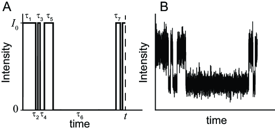
Figure 1: Simplified model for QD intermittency. (A) An individual QD alternates between states “on” and “off” with intensities $I_{0}$ and zero. The sojourn times are $\tau_{j}$ where $j$ is respectively odd and even for “on” and “off” states. The measurement time is $t$. (B) Additional Gaussian noise in the “on” and “off” levels is depicted so that the intensity in these states is not constant but it fluctuates around the mean.

3 Experimental methods: quantum dot imaging

Core-shell CdSe-ZnS quantum dots were purchased from Life Technologies (Qdot 655, Invitrogen). In order to avoid aggregation, the QDs were dispersed in a 1% (w/v) bovine serum albumin solution to a final concentration of 1 nM. A 20-$\mu\mathrm{L}$ drop of this solution was placed on a glass coverslip (Warner Instruments, Hamden, CT) that had been cleaned by sonication in acetone and ethanol. After a 10-minute incubation period the coverslip was thoroughly rinsed with deionized water and dried with nitrogen. We recorded the fluorescence from 1,200 QDs for 22 min at room temperature in a Nikon Eclipse Ti TIRF/widefield fluorescence microscope. QDs were excited by a 488-nm laser line and the emission was collected with a bandpass filter. Images were acquired in a frame-transfer electron multiplying charge-coupled device (EMCCD iXon DU-897, Andor, Belfast UK) at 50 frames per second (exposure time of 20 ms).

QD intensities were measured using an automated algorithm implemented in LabView, which computes the total intensity of each QD. Due to spatial inhomogeneities in excitation power and dot-to-dot variations in quantum yield, different QDs can have varying fluorescence intensities. Thus, we normalize the data so that all intensities lie between zero and one, allowing us to work with a more convenient dimensionless intensity system. For this purpose, we first subtract the minimum value of the intensity along each QD trace and then divide it by the maximum (after subtraction) intensity value.

4 Results

Figure 2A shows the first $600$ seconds of the normalized intensity trace of a typical QD. Usually, QD blinking is analyzed by using a threshold that defines bright and dark states [19, 20, 22]. As mentioned, the threshold determination is rather arbitrary, and in that sense power spectrum analysis is preferred [26]. In agreement with previous observations, the distribution of “off” times is well described by a power law $\psi_{\mathrm{off}}(\tau)\sim\tau^{-(1+\alpha)}$; whereas, the distribution of “on” times shows truncated power-law behavior $\psi_{\mathrm{on}}(\tau)\sim\tau^{-(1+\alpha)}e^{-\tau/\tau_{\mathrm{on}}}$ [20]. In our data we find $\alpha=0.63\pm 0.10$ and $\tau_{\mathrm{on}}=8.5$ s, a time scale that will soon become important.

A representative power spectrum from an individual QD is shown in Fig. 2B. The experimental time of the time trace employed in the computation of this spectrum is 1311 s, i.e., the whole available time. Since the normalized intensity is dimensionless, the PSD has units of $\mathrm{Hz}^{-1}$. Figure 2C shows power spectral densities obtained from averaging the spectra of $1,200$ individual QDs for experimental times of 10 and 1311 s. The spectrum of the long-time trace exhibits two regimes with distinctive $1/f^{\beta}$ behavior. For frequencies below a transition frequency $f_{T}$ we have $S_{t}(f)\sim f^{-\beta_{<}}$ with $\beta_{<}=0.76\pm 0.02$ ($n=1,200$ traces) while above this frequency we have $S_{t}(f)\sim f^{-\beta_{>}}$ with $\beta_{>}=1.393\pm 0.002$. The separation into two regimes is caused by the cutoff that characterizes the “on”-time distribution. Hence, the transition frequency $f_{T}$ is, not surprisingly, of the order of $1/\tau_{\mathrm{on}}$. We will soon compare our experimental findings with the theory for $\beta_{>}$ and $\beta_{<}$, but let us first discuss the transition frequency.

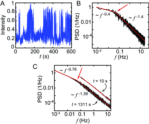
Figure 2: Intermittency in QD fluorescence. (A) Normalized fluorescence intensity of an individual CdSe-ZnS QD, i.e., maximum intensity is unity. (B) PSD of the emission from a single QD measured for 1311 s. (C) Average PSD from the emission of $1,200$ individual QDs. The experimental times are 10 and 1311 s. The short-time spectrum is shifted for clarity. The lines show linear regression of the log-log plot for high and low frequencies according to Eq. (1), and the red arrows point to the transition frequency $f_{T}$.

4.1 The transition frequency $f_{T}$

The existence of a transition frequency implies that the measurement time is crucial. The PSD of the short-time trace (Fig. 2C with $t=10$ s) displays $1/f^{\beta}$ spectrum with a single spectral exponent $\beta_{>}$. On the other hand, long enough measurements yield the transition to a different behavior. Importantly, an observer analyzing short-time traces would reach the conclusion that the power spectrum is non-integrable, since $\beta_{>}>1$. If we wait long enough we eventually observe integrable $1/f$ noise, since $\beta_{<}<1$. In some sense we are lucky to observe this transition: it is detected since the cutoff time $\tau_{\mathrm{on}}$ is on a reasonable time scale.

Previously, Pelton et al. have reported a transition frequency in the power spectrum of blinking QDs [35]. However, that transition has a different nature from the one reported here. In our measurements, a cutoff in “on” sojourn times introduces a transition from $1/f^{2-\alpha}$ to $1/f^{\alpha}$ at low frequencies, i.e., long time behavior, with $f_{T}$ of the order of 0.06 Hz. On the other hand, Pelton et al. find a high frequency transition, i.e., short time behavior, where the spectrum shifts from $1/f^{2-\alpha}$ to $1/f^{2}$ at frequencies above the transition. This high frequency transition was found to be of the order of 100 Hz. The transition to $1/f^{2}$ spectrum was interpreted as short time carrier diffusion yielding, at high frequencies, the power spectrum characteristic of Brownian motion [35].

4.2 Spectral exponents $\beta_{<}$ and $\beta_{>}$

Both exponents $\beta_{<}$ and $\beta_{>}$ are related to $\alpha$. The exponents measured in this study are reported in Table 1 for the benefit of the reader. For frequencies $f>f_{T}$, the cutoff time is of no evident relevance and both states are effectively distributed with power law statistics $\psi(\tau)\sim\tau^{-(1+\alpha)}$. In this regime, theory predicts $\beta_{>}=2-\alpha$ as mentioned above. Since $\alpha=0.63\pm 0.10$, we expect $\beta_{>}=1.37\pm 0.10$, which is similar to the measured exponent. In contrast, for $f<f_{T}$ we must consider the effect of the cutoff time. Thus, we define a modified model, which includes a cutoff in the distribution of “on” times, so that the probability density functions of “on” and “off” sojourn times are different. The important feature of this model is that the mean “on” sojourn time is finite, which modifies the underlying exponents that describe the power spectrum. For this case, one finds $\beta_{<}=\alpha$. Experimentally we find $\beta_{<}=0.76\pm 0.02$ while $\alpha=0.63\pm 0.10$, so small deviations are found. The theoretical sum rule $\beta_{<}+\beta_{>}=2$ is insensitive to the value of $\alpha$ provided that $\alpha<1$, since this implies the divergence of the mean “off” sojourn time, which is the main condition for the observed self-similar behavior.

4.3 Aging exponent $z$

Since the “off” sojourn times are scale free, i.e., mean time is infinite, we expect the amplitude of the power spectrum $A_{t}$ to depend on measurement time. Figure 3A shows averaged power spectra computed for trajectory lengths of $5.1$, $20.5$, $82$, and $1311$ s. As the experimental time $t$ increases, the magnitude of the PSD is not constant but it decreases. To the best of our knowledge, this is the first experimental report explicitly showing that $1/f$ noise in nanoscale systems ages and the concept of stationary $1/f$ noise, so popular in a vast literature, breaks down. Figure 3B shows that the PSD data collapse to a single master trace when multiplied by $t^{0.12}$. According to the theory [33], the power spectrum amplitude scales as $A_{t}\sim t^{-z}$ with the exponent $z=1-\alpha$ both below and above the transition frequency. Thus we expect $z=0.37\pm 0.10$, which is slightly larger than the measured value of the aging exponent $z=0.12$. We will address this deviation with simulations showing that additional noise in the “on” state (see Fig. 1) is important.

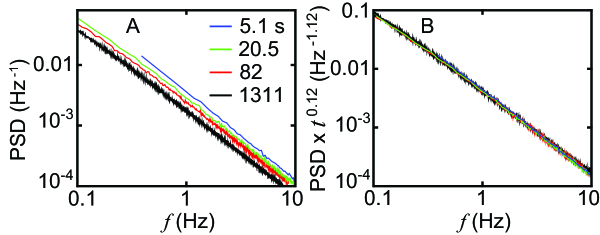
Figure 3: Aging of the power spectrum. (A) Average of 1200 QD power spectral densities for four different experimental times: $5.1$, $20.5$, $82$, and $1311$ s. (B) When the power spectral density is multiplied by an aging factor $t^{z}$ with $z=0.12$, where $t$ is the experimental time, the spectra collapse to a single trace.

4.4 The zero frequency exponent $\omega$

Next, we define the spectrum at zero frequency with

$$S_{t}(0)=S_{t}(f)|_{f=0}=\frac{(\int^{t}_{0}I(\tau)d\tau)^{2}}{t},$$ (5)

and the corresponding exponent $S_{t}(f)|_{f=0}\sim t^{\omega}$. Notice that $S_{t}(0)/t$ is merely the square of the time average $\int_{0}^{t}I(\tau){\rm d}\tau/t$ and its experimental evaluation does not require a fast Fourier transform. For stationary and ergodic processes with non-zero mean intensity we have normal behavior $\omega=1$. On the other hand, if $\omega<1$ the average intensity decays to zero. As shown in Fig. 4A, our measurements yield $\omega\simeq 0.85$, which is a second indication of non-stationarity.

In our system, for long experimental times, the “on” time distribution displays a cutoff and thus the mean “on” time is finite. Therefore, the expected area under the intensity time trace can be estimated to be

$$\langle\int_{0}^{t}I(\tau){\rm d}\tau\rangle=\langle n\rangle\tau_{\mathrm{on}}I_{\mathrm{on}},$$ (6)

where $I_{\mathrm{on}}$ is the intensity in the “on” level and $\langle n\rangle$ is the average number of renewals up to time $t$, i.e., the number of switchings, which is known to increase as $t^{\alpha}$ for waiting “off” times distributed according to power laws [36, 37]. Hence we see that theoretically $S_{t}(f)|_{f=0}\sim t^{2\alpha-1}\simeq t^{0.26}$. Within this model, $\omega=2\alpha-1=0.26$. The measurements in Fig. 4A give $\omega=0.85$, which is surprising since we expect that, at least for long times compared with $\tau_{\rm{on}}$, the cutoff in the “on” times dictate the behavior of the zero frequency spectrum. We will soon remove this mystery by detailed consideration of the effects of noise in the “on” and “off” states using numerical simulations. What becomes clear is that the standard description of blinking systems with a single exponent $\alpha$, so popular in the literature does not describe aging accurately and needs to be expanded. Namely, in our measurements, $\omega$ is not obtained from $\alpha$ in a straightforward way. Hence the standard picture of these systems is challenged.

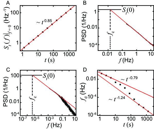
Figure 4: Additional critical exponents describing QD intermittency. (A) Zero-frequency spectrum vs. experimental time. (B-C) Examples showing how the crossover frequency $f_{c}$ is found from the average power spectrum. The horizontal line shows $S_{t}(0)=S_{t}(f)|_{f=0}$. The crossover frequency $f_{c}$ is found by extrapolating $S_{t}(f)\sim{A_{t}f^{-\beta}}$ to the intersection with $S_{t}(0)$. In b the experimental time is $t=5.1$ s, thus $S_{t}(f)\sim{A_{t}f^{-\beta_{>}}}$. On the other hand, in c the time is $t=1311$ s, thus the spectrum shows two different frequency regimes, with $S_{t}(f)\sim{A_{t}f^{-\beta_{<}}}$ for $f<f_{T}$. Note that $f_{c}$ shifts by more than three orders of magnitude between 5.1 and 1311 s. (D) Crossover frequency vs. experimental time. We find that $S_{t}(0)\sim t^{\omega}$ with $\omega=0.85$ and, for short times, $f_{c}\sim t^{-\gamma}$ with $\gamma=-0.79$.

4.5 The crossover frequency $f_{c}\sim t^{-\gamma}$

The transition between the zero frequency spectrum $S_{t}(0)$ and the small but finite frequency behavior $S_{t}(f)\sim f^{-\beta}$, defines a crossover or cutoff frequency $f_{c}$. A crossover frequency is many times assumed to be time independent, though its observation may require extremely long measurement times. For example, in spin glasses the inverse of the cutoff frequency was estimated to be of the order of age of universe [10], and hence it cannot be directly investigated. Given that the PSD ages, we hypothesize the cuttoff frequency also changes with experimental time. We investigate the time dependence of $f_{c}$ within our observation window, which is long in the sense that we measure thousands of transitions between “on” and “off” states. In order to estimate $f_{c}$, we extrapolate Eq. (1) to the intersection with the zero-frequency spectrum, given by Eq. (5), as shown in Figs. 4B and 4C. According to the two state model with i.i.d. sojourn times, $f_{c}\sim t^{-\gamma}$, and $\gamma=1$ [33]. Again this behavior can be derived using scaling arguments. First, we use idealized models, which, by noting that at the crossover frequency $A_{t}f_{c}^{-\beta}=S_{t}(0)$, give $t^{-z}f_{c}^{-(2-\alpha)}\sim t$ for short times and $t^{-z}f_{c}^{-\alpha}\sim t^{2\alpha-1}$ for long times. Surprisingly, these scaling arguments predict $f_{c}\sim 1/t$ for all times, independent of $\tau_{\rm{on}}$. Hence, in this case $\gamma=1$. However, since we already observed deviations in $\omega$ and $z$ from the idealized two-state model, we now use a more general approach using scaling arguments. Here, a second scaling approach relates the various exponents that characterize the process. As before, we employ the relation $A_{t}f_{c}^{-\beta}=S_{t}(0)$, which yields $t^{-z}f_{c}^{-\beta}\sim t^{\omega}$ from the definitions of the various critical exponents. Thus we find

$$\gamma=\frac{\omega+z}{\beta}.$$ (7)

Using measured values for $\omega$, $z$, and $\beta$, we have $\gamma=0.70$ for short times (see Table 1, $\omega=0.85$, $z=0.12$, and $\beta_{>}=1.39$) and $\gamma=1.27$ for long times ($\beta_{<}=0.76$).

For short times, we observe in experiments that the crossover frequency scales with experimental time as $f_{c}\sim t^{-0.79}$ (Fig. 4D). Thus $\gamma=0.79$, which is in good agreement with our general scaling argument approach (Eq. 7) and is consistent with the other critical exponent measurements. For longer measurement times, as seen in Fig. 2C, the low frequency spectrum shifts from $S_{t}(f)\sim 1/f^{\beta_{>}}$ to $S_{t}(f)\sim 1/f^{\alpha}$ where $\beta_{>}>\alpha$. As a consequence of this effect, a transition is observed roughly on the cutoff time $\tau_{\rm{on}}$ and $f_{c}$ decays faster, namely, $\gamma>1$ for $t>\tau_{\rm{on}}$. The behavior can be qualitatively understood, by comparing Figs. 4B and 4C. As the slope of the power spectrum becomes less steep, the crossover is rapidly shifted to smaller frequencies. The value for $\gamma$ at long times is difficult to estimate from our measurements, but it is roughly $\gamma=1.24$. Again, this value is consistent with the measured values of $\omega$ and $z$ as predicted by scaling arguments (Eq. 7).

4.6 Numerical simulations

Deviations between experiments and theory can arise from at least three sources: experimental noise, finite measurement time, and model assumptions not being realistic. Recall that the models neglect any physical noise beyond the switching events (see Fig. 1A) and only attempt to solve for convergences in the long time limits. In particular, the intensity in the “on” and “off” states are not constant; the signal is always fluctuating. To address this issue we turn to numerical simulations. We estimated the four exponents $\beta$, $\omega$, $\gamma$, and $z$ based on numerical simulations. In simulations we add noise to the 0/1 signal (idealized model). Hence, simulations provide additional insight on the analysis. The performed simulations are: PL: Power law; PLN: Power law with noise; PLC: Power law with cutoff (truncated “on” times); and PLCN: Power law with cutoff and noise.

Initially, we generated time series of on/off states with random waiting times drawn from a power-law distribution $\psi(\tau)=\alpha t_{0}^{\alpha}/(\tau+t_{0})^{-(1+\alpha)}$. The constant $t_{0}$ was chosen to be equivalent to the experimental binning time, $t_{0}=20$ ms, and $\alpha=0.63$. We refer to this simulation as PL. In order to add Gaussian noise to the realizations (PLN), the “on” and “off” intensities were transformed at each sampling time into normal random variables $N(0.7,0.04)$ and $N(0.2,0.0064)$, respectively. The sampling time was chosen to be $20$ ms. The variance difference reflects the increased level of noise in the “on” state due to shot noise. To simulate sojourn times distributed according to a power law with cutoff (PLC), the “on” times were drawn from a distribution $\psi(\tau)\sim\tau^{-(1+\alpha)}\mathrm{exp}(-\tau/\tau_{\mathrm{on}})$ and $\tau\geq t_{0}$. The cutoff time was chosen to be $\tau_{\mathrm{on}}=15$ s. Additionally, we performed simulations with both cutoff “on” times and added noise (PLCN). Once noise is added the sojourn time distributions change and estimations of $\alpha$ and $\tau_{\mathrm{on}}$ generally shift toward lower values. Therefore we chose $\tau_{\mathrm{on}}=15$ s in our simulations instead of $8.5$ s as measured in experiments.

The combination of a cutoff time and Gaussian noise has significant effects on the zero-frequency spectrum $S_{t}(0)$ and the crossover frequency $f_{c}$ (Fig. S1). In these simulations, $f_{c}\sim t^{-\gamma}$ with $\gamma<1$ at short times and $\gamma>1$ at times $t>\tau_{\mathrm{on}}$, as observed in the experimental data, and the zero frequency spectrum scales as $S_{t}(0)\sim t^{0.84}$ as well. Table 1 summarizes the exponents found in both experimental data and numerical simulations. Simulation results from a power law distributed two-state model with i.i.d. sojourn times and without noise (PL) are also shown in the Table along with this model’s theoretical predictions. We observe that, while basic non-stationary features of $1/f$ noise agree with recent theory [33], our experimental work shows that introducing noise in the “on”/“off” levels and a finite mean “on” sojourn time is crucial for a complete picture of the power spectrum of blinking QDs.

Table 1: Exponents that describe $1/f$ noise for QD emission (experimental data) and simulations. Results from numerical simulations of two dichotomous random processes are shown: power-law distributed waiting times (PL) and power law with cutoff in “on” times and noise (PLCN). The exponents describe the power spectrum, aging, crossover frequency, and zero-frequency spectrum.

• 			Experimental data	Numerical simulations
  		Theory [33]	QD	PL	PLCN
  $\beta_{>}$	$S_{t}(f)\sim 1/f^{\beta}$	$\beta_{>}=2-\alpha$	1.39	1.38	1.35
  $\beta_{<}$		$\beta_{<}=\alpha$	0.76		0.62
  $z$	$A_{t}\sim 1/t^{z}$	$z=1-\alpha$	0.12	0.36	0.31
  $\gamma$	$f_{c}\sim 1/t^{\gamma}$	$\gamma=1$	0.79a	0.99	0.72a
  $\omega$	$S_{t}(0)\sim t^{\omega}$	$\omega=1^{\rm b}$	0.85	0.99	0.84

• ^a These results hold for $t<\tau_{\mathrm{on}}$. For longer times $\gamma>1$.

• ^bFor long times we have $\omega=2\alpha-1$.

As seen in Table 1, the addition of noise and cutoff on the “on”-time distribution modifies the exponents in such a way that now we obtain better agreement between simulations and measurements. Jeon et al. discussed theoretically the strong influence of noise on the evaluation of physical parameters from data exhibiting power law distributed sojourn times [38]. While that work focused on diffusion of individual molecules in living cells, we can infer the relevance of noise also in our blinking system. Roughly speaking, when power law sojourn times are so broad, the system remains in a state (e.g, “off”) for a time that is of the order of the measurement time. Therefore, the noise level in this long state is of utmost importance for a detailed analysis.

5 Discussion

Our data show that the power spectrum of blinking quantum dots crucially depends on measurement time. We present the first experimental evidence for Mandelbrot’s suggestion that $1/f$ noise is related to non-stationary signals. Our measurements were performed at the nanoscale by measuring single particles, thus removing the problem of averaging a large number of particles, typically found in macroscopic systems. The most common description of macroscopic $1/f$ electronic noise, commonly referred to as the McWhorter model [18, 10], stems from the observation that a superposition of Lorentzian spectra with a broad distribution of relaxation times yield $1/f$ noise. If this philosophy would hold at the nanoscale, by probing an individual molecule, one would expect to measure a Lorentzian spectrum with a well-defined relaxation time. This scenario is not found for blinking quantum dots. Instead, $1/f$ is observed at the nanoscale. Further, the noise exhibits clear non-stationary behavior, i.e., dependence on measurement time. We quantify this non-stationarity with critical exponents. In particular, the aging exponent $z$ shows that the amplitude of the noise decreases as a power law with time. This effect should also be found in other intermittent systems.

The key finding in our work shows that $1/f$ power spectrum of intermittent QDs decays with experimental time, i.e., it ages, and thus the spectrum does not converge in long time measurements as typically assumed for standard stochastic processes. These results agree with previous observations that analyzed blinking in semiconductor quantum dots as a non-stationary process [22, 39]. The description of non-stationary $1/f^{\beta}$ noise we present is vastly different from traditional approaches that characterize it with a single exponent. Besides $\beta$, three additional exponents give the dependence on the measurement time. These exponents describe aging of the power spectrum $A_{t}\sim t^{-z}$, the zero-frequency spectrum $S(f)|_{f=0}\sim t^{\omega}$, and the low cutoff frequency $f_{c}\sim t^{-\gamma}$. Importantly, the appearance of a transition frequency due to a finite mean “on” sojourn time, modifies the underlying exponents that describe the power spectrum.

In an observation time $t$, the total power of the process is $\int_{1/t}^{\infty}S_{t}(f){\rm d}f$ where $1/t$ is the lowest measured frequency. For a process with power spectrum $S(f)=A/f^{\beta}$ with $1<\beta<2$ the total power diverges as time increases, due to the low frequency behavior. In contrast, if $S(f)=A/f^{\beta}$ and $0<\beta<1$, the total power diverges due to the high frequency behavior of the spectrum. We observe that in QDs, two different phenomena limit the increase of total power. First, below the transition frequency $f_{T}$, we find $\beta<1$ due to the cutoff in the “on” sojourn times and hence the spectrum is integrable at low frequencies. For large frequencies $\beta>1$ hence it is integrable also at high frequencies. Second, as the observation time progresses, the amplitude of the power spectrum decreases with $A_{t}\sim t^{-z}$, so that $S_{t}(f)\rightarrow 0$ in the limit $t\rightarrow\infty$. Both these findings maintain the total power finite. More precisely, if one measures for times that are shorter than $\tau_{\mathrm{on}}$ and hence the transition to an integrable spectrum is not detected at low frequencies, the decrease of the spectrum with time ensures that the total area under the power spectrum does not blow up. This will become particularly important in the limit of weak laser field excitation and low temperatures, where $\tau_{\mathrm{on}}$ becomes extremely large [20] and a single regime in the power spectrum holds for all observable time scales, i.e., the transition frequency $f_{T}$ is not observed within the available frequency range. We measure the total power by integrating the power spectral density as defined above and indeed, we obtain a finite value which is not diverging, i.e. it is bound, though convergence is slow (Fig. S2). The aging of the spectrum ensures that total power of the system will not diverge, hence, our observations help in removal of a long-standing paradox of physics [3].

By resorting to numerical simulations, we find that a model that includes both a cutoff in “on” sojourn times and noise in each state (PLCN model) describes more accurately the experimental results obtained. These simulations emphasize the influence of noise within the “on” and “off” states and power low with a cut-off distribution. However, the value of the aging exponent $z$ still remains somewhat far from our experimental observations. The aging exponent in simulations is estimated to be $z=0.31$, while in experiments $z=0.12$. We can speculate there are two reasons responsible for the observed discrepancy. First, these models still assume the existence of solely two levels. Recent experiments point to the existence of intermediate states in the emission from core-shell QDs [40, 41]. The occurrence of multiple states has been described both in terms of blinking processes that are faster than the time resolution of the experiment (as is the case in our experiments) [42] and in terms of multiple physical states within the core-shell quantum dot [41, 43]. Nevertheless, the main aspects of the non-stationarity described here are expected to hold for the multiple level system as long as at least one of the states is governed by a scale-free power law distribution. Second, a different phenomenon that could affect the measured critical exponents is noise in the QD levels that is not Gaussian. The influence of non-Gaussian noises can of course have striking consequences in the properties of a stochastic process.

In our approach the exponents were analyzed in a way that is reminiscent of critical behavior, with scaling relations showing the exponents are dependent on each other and with different behaviors below and above a transition frequency $f_{T}\simeq 1/\tau_{\mathrm{on}}$. These results are relevant to a broad range of systems displaying power law intermittency [44, 45, 29, 17, 16]. Further, power law sojourn times, which is the basic ingredient leading to the observed non-stationary spectrum in blinking quantum dots, are widespread and are found in glassy systems [46, 47] and anomalous diffusion in live cell environments and other complex systems [48, 49, 50, 51, 52]. Therefore, the measured exponents could be a general feature of many noisy signals. Finally, the traditional characterization of blinking quantum dots with a single exponent $\alpha$ is shown to be limited and to hide interesting physics described by different critical exponents.

6 Conclusions

Our experiments show how the analysis of noise in blinking quantum dots reveals rich physical behavior described by four critical exponents. This is vastly different from traditional approaches that characterized power spectrum of $1/f^{\beta}$ noise with a single exponent $\beta$. The exponent $z$ describes the aging of the spectrum with measurement time, showing a decrease of the noise level as the measurement time increases. The exponent $\beta$ describes the $1/f^{\beta}$ noise as in many previous studies, however we find two such exponents $\beta_{<}$ and $\beta_{>}$, below and above the transition frequency $f_{T}$. The zero frequency exponent $\omega$ describes the time average of the intensity, which is essentially related to ergodicity and yields further information on the non-stationarity of the process. The exponent $\gamma$ describes the crossover from zero frequency to $1/f^{\beta}$. We hope that our work will promote measurements of exponents of $1/f^{\beta}$ spectrum, since they reveal the true complexity of the observed phenomena.

References

- [1] Hooge FN (1972) Discussion of recent experiments on 1/f noise. Physica 60:130.
- [2] Eliazar I, Klafter J (2009) A unified and universal explanation for Lévy laws and 1/f noises. Proc. Natl. Acad. Sci. USA 106:12251–12254.
- [3] Mandelbrot B (1967) Some noises with spectrum, a bridge between direct current and white noise. IEEE Trans. Inform. Theory 13:289.
- [4] Dutta P, Horn PM (1981) Low-frequency fluctuations in solids: 1/f noise. Rev. Mod. Phys. 53.
- [5] Sornette A, Sornette D (1989) Self-organized criticality and earthquakes. Europhys. Lett. 9:197.
- [6] Csabai I (1994) 1/f noise in computer network traffic. J. Phys. A: Math. Gen. 27:L417.
- [7] Halley JM (1996) Ecology, evolution and 1/f noise. Trends in Ecology & Evolution 11:33–37.
- [8] Gilden DL, Thornton T, Mallon MW (1995) 1/f noise in human cognition. Science 267:1837–1839.
- [9] Keshner MS (1982) 1/f noise. Proc. IEEE 70:212.
- [10] Kogan S (1996) Electronic noise and fluctuations in solids. (Cambridge Univ. Press, New York).
- [11] Johnson JB (1925) The Schottky effect in low frequency circuits. Phys. Rev. 26:71.
- [12] Caloyannides MA (1974) Microcycle spectral estimates of 1/f noise in semiconductors. J. Appl. Phys. 45:307.
- [13] Mandelbrot BB, Wallis JR (1969) Some long-run properties of geophysical records. Water resources research 5:321–340.
- [14] Bezrukov SM, Winterhalter M (2000) Examining noise sources at the single-molecule level: 1/f noise of an open maltoporin channel. Phys. Rev. Lett. 85:202.
- [15] Siwy Z, Fuliński A (2002) Origin of 1/f noise in membrane channel currents. Phys. Rev. Lett 89:1.
- [16] Krapf D (2013) Nonergodicity in nanoscale electrodes. Phys. Chem. Chem. Phys. 15:459.
- [17] Bizzarri AR, Cannistraro S (2013) 1/fα noise in the dynamic force spectroscopy curves signals the occurrence of biorecognition. Phys. Rev. Lett. 110:048104.
- [18] Balandin AA (2013) Low-frequency 1/f noise in graphene devices. Nat. Nanotechnol. 8:549–555.
- [19] Kuno M, Fromm DP, Hamann HF, Gallagher A, Nesbitt DJ (2000) Nonexponential “blinking” kinetics of single CdSe quantum dots: A universal power law behavior. J. Chem. Phys. 112:3117.
- [20] Shimizu KT et al. (2001) Blinking statistics in single semiconductor nanocrystal quantum dots. Phys. Rev. B 63:205316.
- [21] Frantsuzov PA, Volkán-Kacsó S, Jankó B (2013) Universality of the fluorescence intermittency in nanoscale systems: experiment and theory. Nano Lett. 13:402.
- [22] Brokmann X et al. (2003) Statistical aging and nonergodicity in the fluorescence of single nanocrystals. Phys. Rev. Lett. 90:120601.
- [23] Frantsuzov P, M. Kuno BJ, Marcus RA (2008) Universal emission intermittency in quantum dots, nanorods and nanowires. Nat. Phys. 4:519.
- [24] Stefani FD, Hoogenboom JP, Barkai E (2009) Beyond quantum jumps: blinking nanoscale light emitters. Phys. Today 2:34.
- [25] Pelton M, Grier DG, Guyot-Sionnest P (2004) Characterizing quantum-dot blinking using noise power spectra. Appl. Phys. Lett. 85:819.
- [26] Crouch CH et al. (2010) Facts and artifacts in the blinking statistics of semiconductor nanocrystals. Nano Lett. 10:1692.
- [27] Nirmal M et al. (1996) Fluorescence intermittency in single cadmium selenide nanocrystals. Nature 338:802804.
- [28] Manneville P (1980) Intermittency, self-similarity and 1/f spectrum in dissipative dynamical systems. J. Phys. (Paris) 41:1235.
- [29] Silvestri L, Fronzoni L, Grigolini P, Allegrini P (2009) Event-driven power-law relaxation in weak turbulence. Phys. Rev. Lett. 102:014502.
- [30] Hoogenboom JP, Hernando J, van Dijk EM, van Hulst NF, García-Parajo MF (2007) Power-law blinking in the fluorescence of single organic molecules. Chem. Phys. Chem. 8:823–833.
- [31] Niemann M, Szendro IG, Kantz H (2010) 1/fβ noise in a model for weak ergodicity breaking. Chem. Phys. 375:370–377.
- [32] Margolin G, Barkai E (2006) Nonergodicity of a time series obeying Lévy statistics. J. Stat. Phys. 122:137.
- [33] Niemann M, Kantz H, Barkai E (2013) Fluctuations of 1/f noise and the low-frequency cutoff paradox. Phys. Rev. Lett. 110:140603.
- [34] Godec A, Metzler R (2013) Linear response, fluctuation-dissipation, and finite-system-size effects in superdiffusion. Phys. Rev. E 88:012116.
- [35] Pelton M, Smith G, Scherer NF, Marcus RA (2007) Evidence for a diffusion-controlled mechanism for fluorescence blinking of colloidal quantum dots. Proc. Natl. Acad. Sci. USA 104:14249–14254.
- [36] Godrèche C, Luck JM (2001) Statistics of the occupation time of renewal processes. J. Stat. Phys. 104:489–524.
- [37] Klafter J, Sokolov IM (2011) First Steps in Random Walks. (Oxford Univ. Press, New York), p. 49.
- [38] Jeon JH, Barkai E, Metzler R (2013) Noisy continuous time random walks. J. Chem. Phys. 139:121916.
- [39] Messin G, Hermier J, Giacobino E, Desbiolles P, Dahan M (2001) Bunching and antibunching in the fluorescence of semiconductor nanocrystals. Opt. Lett. 26:1891–1893.
- [40] Zhang K, Chang H, Fu A, Alivisatos AP, Yang H (2006) Continuous distribution of emission states from single CdSe/ZnS quantum dots. Nano Lett. 6:843–847.
- [41] Spinicelli P et al. (2009) Bright and grey states in CdSe-CdS nanocrystals exhibiting strongly reduced blinking. Phys. Rev. Lett. 102:136801.
- [42] Galland C et al. (2011) Two types of luminescence blinking revealed by spectroelectrochemistry of single quantum dots. Nature 479:203.
- [43] Amecke N, Cichos F (2011) Intermediate intensity levels during the emission intermittency of single cdse/zns quantum dots. J. Luminesc. 131:375–378.
- [44] Zumofen G, Klafter J (1993) Power spectra and random walks in intermittent chaotic systems. Physica D 69:436.
- [45] Scher H, Margolin G, Metzler R, Klafter J, Berkowitz B (2002) The dynamical foundation of fractal stream chemistry: The origin of extremely long retention times. Geophys. Res. Lett. 29:1061.
- [46] Bouchaud JP (1992) Weak ergodicity breaking and aging in disordered systems. J. Phys. I (France) 2:1705.
- [47] Burov S, Metzler R, Barkai E (2010) Aging and nonergodicity beyond the Khinchin theorem. Proc. Natl. Acad. Sci. USA 107:13228–13233.
- [48] Bouchaud JP, Georges A (1990) Anomalous diffusion in disordered media: statistical mechanisms, models and physical applications. Phys. Rep. 195:127–293.
- [49] Metzler R, Klafter J (2004) The restaurant at the end of the random walk: recent developments in the description of anomalous transport by fractional dynamics. J. Phys. A: Mathematical and General 37:R161.
- [50] Weigel AV, Simon B, Tamkun MM, Krapf D (2011) Ergodic and nonergodic processes coexist in the plasma membrane as observed by single-molecule tracking. Proc. Natl. Acad. Sci. USA 108:6438–6443.
- [51] Tabei SA et al. (2013) Intracellular transport of insulin granules is a subordinated random walk. Proc. Natl. Acad. Sci. USA 110:4911–4916.
- [52] Burov S et al. (2013) Distribution of directional change as a signature of complex dynamics. Proc. Natl. Acad. Sci. USA 110:19689–19694.