Line driven winds and the UV turnover in AGN accretion discs

Abstract

AGN SEDs generally show a turnover at $\lambda\sim 1000$Å, implying a maximal Accretion Disc (AD) temperature of $T_{\rm max}\sim 50,000$K. Massive O stars display a similar $T_{\rm max}$, associated with a sharp rise in a line driven mass loss $\dot{M}_{\rm wind}$ with increasing surface temperature. AGN AD are also characterized by similar surface gravity to massive O stars. The $\dot{M}_{\rm wind}$ of O stars reaches $\sim 10^{-5}M_{\odot}~{}{\rm yr}^{-1}$. Since the surface area of AGN AD can be $10^{6}$ larger, the implied $\dot{M}_{\rm wind}$ in AGN AD can reach the accretion rate $\dot{M}$. A rise to $\dot{M}_{\rm wind}\sim\dot{M}$ towards the AD center may therefore set a similar cap of $T_{\rm max}\sim 50,000$K. To explore this idea, we solve the radial structure of an AD with a mass loss term, and calculate the implied AD emission using the mass loss term derived from observations of O stars. We find that $\dot{M}_{\rm wind}$ becomes comparable to $\dot{M}$ typically at a few tens of $GM/c^{2}$. Thus, the standard thin AD solution is effectively truncated well outside the innermost stable orbit. The calculated AD SED shows the observed turnover at $\lambda\sim 1000$Å, which is weakly dependent on the AGN luminosity and black hole mass. The AD SED is generally independent of the black hole spin, due to the large truncation radius. However, a cold AD (low $\dot{M}$, high black hole mass) is predicted to be windless, and thus its SED should be sensitive to the black hole spin. The accreted gas may form a hot thick disc with a low radiative efficiency inside the truncation radius, or a strong line driven outflow, depending on its ionization state.

1 Introduction

The optical-UV emission in AGN is most likely the signature of accretion on to the central massive black hole through a thin Accretion Disc (AD, Shields 1978; Malkan 1983 and citations thereafter). Malkan & Sargent (1982) noted that the UV emission shows a turnover characteristic of a $T_{\rm max}\sim 30,000$K blackbody. Following studies of larger samples showed this is a general trend in AGN, where the SED shows a turnover from a spectral slope of $\alpha\sim-0.5$ ($F_{\nu}\propto\nu^{\alpha}$) at $\lambda>1000$Å, to $\alpha\sim-1.5$ to $-2$ at $\lambda<1000$Å (Zheng et al. 1997; Telfer et al. 2002; Shang et al. 2005; Barger & Cowie 2010; Shull et al. 2012; cf. Scott et al. 2004), which extends to $\sim 1$ keV (Laor et al. 1997). The turnover at $\lambda<1000$Å, which corresponds to a blackbody with $T_{\rm max}\sim 50,000$K, is in contradiction with the thin local blackbody AD models, which predict peak emission $\nu_{\rm peak}\propto(\dot{m}/M)^{1/4}$, where $M$ is the black hole mass, and $\dot{m}\equiv L/L_{\rm Edd}$ is the luminosity in Eddington units. Thus, $\nu_{\rm peak}$ should range over more than an order of magnitude, as broad line AGN extend over the range $\dot{m}=0.01-1$ and $M=10^{6}-10^{10}M_{\odot}$, which is in contrast with the small range observed (e.g. Shang et al. 2005; Davis & Laor 2011, hereafter DL11). For example, some models predict a peak at $\nu_{\rm peak}>10^{16}$ (e.g. Hubeny et al. 2001, DL11), while objects with such SEDs appear to be extremely rare (e.g. Done et al. 2012). Furthermore, high $\dot{m}/M$ AD models predict significant soft X-ray thermal emission, which is also not observed (Laor et al. 1997), which again implies the expected thermal emission from the inner hottest parts of the AD is missing.

The extreme UV (EUV) emission spectral shape can also be constrained based on various line ratios. The analysis of Bonning et al. (2013) of a sample of AGN reveals similar observed line ratios, again indicating similar EUV SEDs, and an absence of the dependence of the EUV emission on the predicted maximum thin AD temperature in each object.

In contrast, the SED of AD around stellar mass black holes, which peak in the X-ray regime, matches observations remarkably well, in particular near the peak emission which originates from the hottest innermost AD region (Davis et al. 2005; 2006). The match is accurate enough that it can be used to determine the black hole spin (e.g. McClintock et al. 2011).

What prevents AD in AGN from generally reaching $T_{\rm max}\gg 50,000$K? The universality of the observed $\nu_{\rm peak}$ suggests it is a local process in the AGN AD atmosphere, most likely related to an atomically driven process. This process should be effective at $T\sim 50,000$ K, and absent at $T\sim 10^{7}$ K, relevant to AD around stellar mass black holes.

Interestingly, main sequence stars show a similar maximum temperature. The hottest O stars also do not generally reach beyond $\sim 50,000$ K (e.g. Howarth & Prinja 1989). Massive O stars produce a strong wind with a high mass loss, $\dot{M}_{\rm wind}$, which can reach $10^{-5}M_{\odot}~{}{\rm yr}^{-1}$ in the most luminous O stars with a luminosity $L_{*}>10^{6}L_{\odot}$. Such stars have a mass of $M_{*}\sim 50-100M_{\odot}$, and thus loose a significant fraction of their mass on a time-scale $t_{\rm wind}=M_{*}/\dot{M}_{\rm wind}\sim 5-10$ Myr, which is comparable to their lifetime.

Is this $\dot{M}_{\rm wind}$ regulation of the hottest and most massive O stars relevant to AGN? Can this mechanism explain the similar $T_{\rm max}$ observed in AGN AD and in O stars? The local structure of a stellar atmosphere is mostly set by the local flux, i.e. the effective temperature $T_{\rm eff}$, and by the surface gravity $g$. AGN AD have $T_{\rm eff}\sim 10^{4}-10^{5}$ K at their inner regions, and $g$ at the disc surface is set by the balance of radiation pressure and gravity. Thus, the local flux and $g$ are always at the Eddington limit in the vertical direction. In O stars, the local flux and $g$ also reach close to the Eddington limit. The radius of O stars is $\sim 10^{12}$ cm. The radius of the UV emitting region in luminous AGN AD is $\sim 10^{15}$ cm, i.e. a $10^{6}$ larger surface area. Thus, if the mass loss per unit surface area reaches similar values in O stars and in AGN, given their similar $T_{\rm max}$ and $g$, then the total $\dot{M}_{\rm wind}$ from the AGN AD where $T\sim 50,000$ K can reach $10M_{\odot}~{}{\rm yr}^{-1}$, which can exceed the accretion rate $\dot{M}$. The value of $T_{\rm max}$ in AGN AD may then be set by the radius at which the thin disc solution must break down as $\dot{M}_{\rm wind}>\dot{M}$.

Below we explore this suggestion more quantitatively. In §2 we derive the mass loss per unit surface area in stars as a function of the atmospheric properties. In §3 we provide a simple analytic estimate of the innermost disc radius, and the implied $T_{\rm max}$ in AGN AD, based on the O stars mass loss. In §4 we derive revised equation for the radial AD structure for a thin AD + wind. In §5 we provide numerical solutions for the revised thin AD radial structure. In §6 we derive the AD SED using various approximations. The results are discussed in §7, and the main conclusions are summarized in §8.

2 Stellar mass loss

Below we use the stellar $\dot{M}_{\rm wind}(L_{*})$ relation to derive a relation between the mass loss per unit area, $\dot{\Sigma}$, and the locally emitted flux per unit area (i.e $T_{\rm eff}$). We assume this relation applies to AGN AD, and use the AD expression for $T_{\rm eff}(R)$ to derive $\dot{\Sigma}(R)$, where $R$ is the radius. We then integrate over the AD surface area to derive the cumulative $\dot{M}_{\rm wind}(R)$, and derive $R_{\rm eq}$ at which $\dot{M}_{\rm wind}(R_{\rm eq})=\dot{M}$, where $\dot{M}$ is the accretion rate coming in from infinity. This radius forms the effective inner thin AD boundary, and sets the maximum thin disc temperature, $T_{\rm max}=T_{\rm eff}(R_{\rm eq})$.

Observations of O stars yield the following tight relation between $\dot{M}_{\rm wind}$ and $L_{*}$,

$$\log\dot{M}_{\rm wind}/M_{\odot}~{}{\rm yr}^{-1}=1.69\log L_{*}/L_{\odot}-15.4,$$ (1)

derived in the range $4.5<\log L_{*}/L_{\odot}<6.5$, (Howarth & Prinja 1989), which corresponds to an effective temperature in the range $30,000<\log T_{\rm eff}<50,000$ K, where the O stars range from main sequence to supergiants. Howarth & Prinja (1989) list the stellar radius $R_{*}$ for their sample of 201 stars, which we use to derive the mass loss rate per unit area, $\dot{\Sigma}$, for each star. Figure 1 (top panel) presents the derive best fit linear relation of $\dot{\Sigma}$ and $F/F_{\odot}$,

$$\log\dot{\Sigma}=1.9\log F/F_{\odot}-15.7,$$ (2)

where $\dot{\Sigma}$ is measured here and below in units of $M_{\odot}~{}{\rm yr}^{-1}R_{\odot}^{-2}$, and $F/F_{\odot}$ is the flux in solar flux units, which equals $(T_{\rm eff}/5774)^{4}$. The relation has a scatter of 0.28 in $\log\dot{\Sigma}$ at a given $T_{\rm eff}$ (see Figure 1).

Solutions for the atmospheric structure are set by $T_{\rm eff}$ and $g$. Thus, although the global $\dot{M}_{\rm wind}$ in stars is set by $L_{*}$ only, the local $\dot{\Sigma}$ is likely set by both $T_{\rm eff}$ and $g$. Figure 1 (middle panel) shows the derived best fit relation of $\dot{\Sigma}$ vs. $F$ and $g$

$$\log\dot{\Sigma}=2.32\log F/F_{\odot}-1.11\log g/g_{\odot}-17.72,$$ (3)

where $g/g_{\odot}$ is the surface gravity in solar units. Indeed, the relation is significantly tighter, and the scatter reduces to 0.06.

This relation is consistent with the line driven winds solution (Castor et al. 1975; hereafter CAK) which yields, to a good approximation,

$$\dot{M}_{\rm wind}\propto[M_{*}(1-\Gamma)]^{(\alpha-1)/\alpha}L_{*}^{1/\alpha},$$ (4)

where $\Gamma=L_{*}\sigma_{\rm es}/4\pi cGM_{*}$ represents $L_{*}$ in Eddington units, and $\alpha$ describes the power law dependence of the force multiplier $M$ on the electron scattering optical depth, $t$, from the surface of the atmosphere, $M\propto t^{-\alpha}$. Since $\alpha\simeq 0.5$ (e.g. Lamers & Cassinelli 1999), and $\Gamma<0.5$ for O stars (Figure 1, lower panel), we get in the limit $\Gamma\ll 1$ that $\dot{M}_{\rm wind}\propto M_{*}^{-1}L_{*}^{2}$. Now, using the local quantities, $g\propto M_{*}/R^{2}$, and $F\propto L_{*}/R^{2}$, we derive $\dot{\Sigma}\propto g^{-1}F^{2}$, which is close to the relation found above (equation 3).

Although the $\dot{\Sigma}(F,g)$ relation (equation 3) is significantly tighter than the $\dot{\Sigma}(F)$ relation (equation 2), its applicability to AGN AD is not clear. In the radiation pressure dominated part of AD, relevant to AGN AD at small $R$, $\Gamma=1$ at the disc surface, and the CAK expression for $\dot{M}_{\rm wind}$ (equation 4) formally diverges. However, in AD the dynamics is different, as $g\propto z$ and $F$ is constant for $z\ll R$, in contrast with stars where both $g$ and $F$ are $\propto 1/R^{2}$, so $\Gamma>1$ does not lead to divergence as in the stellar case. We therefore use below both the $\dot{\Sigma}(F,g)$ and the $g$ averaged $\dot{\Sigma}(F)$ relation, to get some indication of possible $\dot{M}_{\rm wind}$ values.

We note in passing that additional $\dot{\Sigma}(F,g)$ relations can be derived from various theoretical calculations presented by Vink et al. (2000) and Lucy (2010). For the sake of simplicity we use only the observationally derived relations given above.

Figure 1: Upper panel: The relation between the mass loss per unit area $\dot{\Sigma}$ and the local flux $F$, derived from the measured total mass loss, luminosity, and radius for 201 O stars tabulated by Howarth & Prinja (1989). The solid line marks the $\dot{\Sigma}(F)$ relation used for AGN AD. Middle panel: The relation between $\dot{\Sigma}$ and both $F$ and $g$. This rather tight relation follows the predicted CAK relation between $\dot{M}$ and both $L_{*}$ and $M_{*}$, ignoring the $1-L/L_{\rm Edd}$ term in the CAK solution. The solid line marks the $\dot{\Sigma}(F,g)$ relation used for AGN AD. Although this relation is significantly tighter than the $\dot{\Sigma}(F)$ relation derived in the upper panel, this relation is expected to break in stars at the Eddington limit, which produces the same local conditions as in AD atmosphere. Also, the value of $g$ in the standard AD solution assumes only pure electron scattering opacity, an assumption which breaks down in AGN AD. Lower panel: The relation between the surface gravity and the local flux for the 201 O stars. The solid line shows relation in an atmosphere supported by radiation pressure, with an electron scattering opacity, as expected in the inner part of an AGN AD. In O star atmospheres the radiation force induced by electron scattering supports up to a half of the local gravity.

3 Analytic estimate of $T_{\rm max}$

Below we derive the integrated AD wind

$$\dot{M}_{\rm wind}(R)=\int_{\infty}^{R}4\pi R\dot{\Sigma}dR.$$ (5)

based on the relation derived above for $\dot{\Sigma}$ (eqs. 2 & 3). We find the radius $r_{\rm eq}$ where $\dot{M}_{\rm wind}=\dot{M}$, and the thin disc solution likely terminates. We then find the local blackbody surface temperature $T_{\rm max}$ at $r_{\rm eq}$, i.e. the hottest temperature for the thin disc solution.

The flux emitted per unit area from the surface of a thin AD (Shakura & Sunyaev 1973, hereafter SS73) is

$$F=\frac{3}{8\pi}\frac{G\dot{M}M}{R^{3}}f(R,M,a_{*})$$ (6)

where $R$ is the radius, and $f(R,M,a_{*})$ is a dimensionless factor set by the inner boundary condition, and the relativistic effects (Novikov & Thorne 1973; Riffert & Herold 1995), and is of order unity at radii a factor of few larger than the inner boundary. We assume $f(R,M,a_{*})=1$ below. We use the dimensionless radius, $r\equiv R/R_{g}$, where $R_{g}\equiv GM/c^{2}$, which gives

$$F=\frac{3c^{6}}{8\pi G^{2}}\frac{\dot{M}}{M^{2}r^{3}},$$ (7)

or equivalently

$$F/F_{\odot}=5\times 10^{8}\dot{M_{1}}m_{8}^{-2}r^{-3},$$ (8)

using the relations $M=10^{8}m_{8}~{}M_{\odot}$, $\dot{M}=\dot{M_{1}}~{}M_{\odot}~{}yr^{-1}$, and a solar flux $F_{\odot}=6.3\times 10^{10}~{}{\rm erg}~{}{\rm s}^{-1}~{}{\rm cm}^{-2}$.

3.1 Derivation for $\dot{\Sigma}(F)$

We now use the AD expression for the local $F$ to derive the expected local $\dot{\Sigma}(F)$ in AD. For convenience, we express $R$ in equation (5) in solar radii, $R^{\prime}=R/R_{\odot}$ where $R_{\odot}=6.93\times 10^{10}$ cm, or equivalently $R^{\prime}=213m_{8}r$. Thus, equation (5) can be expressed as

$$\dot{M}_{\rm wind}(r)=5.69\times 10^{5}m_{8}^{2}\int_{\infty}^{r}r\dot{\Sigma}(F)dr.$$ (9)

We now insert equation (8) into equation (2), and get an expression for the local disc $\dot{\Sigma}$

$$\dot{\Sigma}=0.673\dot{M_{1}}^{1.9}m_{8}^{-3.8}r^{-5.7},$$ (10)

which implies a sharp rise in the local mass loss towards the center. The integrated mass loss is then

$$\dot{M}_{\rm wind}(r)=4.7\times 10^{5}m_{8}^{-1.8}\dot{M_{1}}^{1.9}r^{-3.7}.$$ (11)

Thus, $\dot{M}_{\rm wind}(r)=\dot{M}$ at

$$r_{\rm eq}=34.1m_{8}^{-0.48}\dot{M_{1}}^{0.24},$$ (12)

which forms the effective inner boundary of the thin disc solution. Note that the wind is sharply confined towards $r_{\rm eq}$, as 50% of $\dot{M}_{\rm wind}$ is launched inside $1.2r_{\rm eq}$ and 92% inside $2r_{\rm eq}$. The surface effective temperature of a thin AD is (from equation 8)

$$T_{\rm eff}=8.6\times 10^{5}\dot{M_{1}}^{1/4}m_{8}^{-1/2}r^{-3/4}~{}{\rm K}.$$ (13)

Thus, the AD temperature at $r_{\rm eq}$ is

$$T_{\rm max}=6.1\times 10^{4}\dot{M_{1}}^{0.07}m_{8}^{-0.14}~{}{\rm K}.$$ (14)

Assuming an accretion efficiency of 10%, the bolometric luminosity is $L=5.67\times 10^{45}\dot{M_{1}}$, and $L$ in Eddington luminosity units is $\dot{m}=0.44\dot{M_{1}}m_{8}^{-1}$. The above expression is equivalent to

$$T_{\rm max}=6.5\times 10^{4}(\dot{m}/m_{8})^{0.07}~{}{\rm K},$$ (15)

compared to the $T_{\rm eff}\propto(\dot{m}/m_{8})^{0.25}$ dependence in the SS73 solution (from equation 13 with $\dot{M_{1}}$ replaced by $m_{8}\dot{m}$). This simplistic derivation yields that line driven winds from thin accretion discs in AGN produce an inner boundary with a maximum temperature of $\sim(5-6)\times 10^{4}$ K, with a weak dependence on $\dot{m}$ and $m_{8}$. A change by a factor of $10^{4}$ in $\dot{m}/m_{8}$ changes $T_{\rm max}$ by only a factor of two. The wind truncation then explains both the observed position of the UV peak, and its uniformity, with no free parameters.

3.2 Derivation for $\dot{\Sigma}(F,g)$

Below we repeat the above derivation using the above expression for $\dot{\Sigma}(F,g)$ (equation 3).

We first need to derive the vertical component of gravity, $g$, at the disc surface. The inner AD is supported by radiation pressure, where the source of opacity is assumed to be dominated by electron scattering. Thus, $g$ in hydrostatic equilibrium is

$$g=F\kappa_{\rm es}/c,$$ (16)

where $\kappa_{\rm es}=0.34~{}{\rm g}~{}{\rm cm}^{-2}$ is the electron scattering opacity of fully ionized gas. Or, in dimensionless units

$$g/g_{\odot}=2.6\times 10^{-5}F/F_{\odot},$$ (17)

where $g_{\odot}=2.74\times 10^{4}$ cm s^-2 on the solar surface. Thus, since $g$ is set by $F$, equation (3) can be rewritten in the form

$$\log\dot{\Sigma}=1.21\log F/F_{\odot}-12.63,$$ (18)

i.e. a weaker dependence on $F$, compared to the $\dot{\Sigma}(F)$ relation (equation 2). Inserting the AD expression for $F$ (equation 8), into the above expression yields,

$$\dot{\Sigma}=7.87\times 10^{-3}\dot{M_{1}}^{1.21}m_{8}^{-2.42}r^{-3.63},$$ (19)

and following the integration we get

$$\dot{M}_{\rm wind}(r)=2.75\times 10^{3}m_{8}^{-0.42}\dot{M_{1}}^{1.21}r^{-1.63}.$$ (20)

We thus get a significantly weaker rise in $\dot{M}_{\rm wind}$ with decreasing $r$, compared to the one derived from the $\dot{\Sigma}(F)$ relation (equation 11). We now get

$$r_{\rm eq}=129m_{8}^{-0.26}\dot{M_{1}}^{0.13}.$$ (21)

Note that in this case the wind is somewhat less sharply confined towards $r_{\rm eq}$, compared to the $\dot{\Sigma}(F)$ case. Here, 50% of $\dot{M}_{\rm wind}$ is launched inside $1.5r_{\rm eq}$ and 92% inside $4.7r_{\rm eq}$, compared to $1.2r_{\rm eq}$ and $2r_{\rm eq}$ in the $\dot{\Sigma}(F)$ case. We also get

$$T_{\rm max}=2.25\times 10^{4}\dot{M_{1}}^{0.153}m_{8}^{-0.305}~{}{\rm K}.$$ (22)

or

$$T_{\rm max}=1.99\times 10^{4}(\dot{m}/m_{8})^{0.153}~{}{\rm K},$$ (23)

which is steeper than the $(\dot{m}/m_{8})^{0.07}$ dependence derived for the $\dot{\Sigma}(F)$ solution (equation 15), but is still flatter than the SS73 dependence of $(\dot{m}/m_{8})^{0.25}$. The value of $T_{\rm max}$ here is lower than for the $\dot{\Sigma}(F)$ solution.

The wind flux is inversely correlated with $g$ (equation 3). The value of $g$ in hydrostatic equilibrium depends linearly on the gas opacity (equation 16). The electron scattering opacity used here is the minimal opacity for ionized gas. The additional contribution from line opacity increases $g$, and thus decreases $\dot{\Sigma}$. As a result, the disc may extend further inwards, and thus reach a higher temperature than derived above (eqs. 22, 23).

4 The Navier-Stokes equations for an AD with mass loss

The above estimates suggest that line driven winds from AGN AD prevent the formation of the hot inner AD regions with $T>10^{5}$ K, which may explain the uniformity of the FUV SED of AGN. However, these estimate are rather crude, as the expression used for $F$ (equation 8) ignores the reduction in $\dot{M}$ due to the wind mass loss. Below we derive the AD structure, based on the mass, momentum and energy continuity equations, including a wind mass loss term. We then calculate the revised AD SED, first using the local blackbody approximation, and then using the stellar atmospheric solution code TLUSTY (Hubeny & Lanz, 1995; Hubeny et al., 2000).

The derivation below is for a viscous flow, described by the Navier-Stokes equations. We use cylindrical coordinates, $R,z,\phi$, and assume axial symmetry (no $\phi$ dependence). We further assume the $R$ and $z$ solutions are separable, which is likely valid in the thin disc approximation, and we solve for the radial dependence only. The solution below yields the radial dependence of the vertically integrated viscous torque $W_{R\phi}(R)$, which is required in order to get a steady state solution. This quantity, together with $\Omega(R)$ - the angular velocity radial dependence, uniquely determine $F(R)$. The physical origin of $W_{R\phi}(R)$ is an open question, heuristically addressed by the $\alpha$ disc model (SS73). In ionized accretion discs, it is now widely believed that angular momentum transport is provided by magnetorotational turbulence (Balbus & Hawley, 1998), which when averaged over time and the vertical extent of the disc, seems to be reasonably approximated by an $\alpha$-disc solution (Balbus & Papaloizou, 1999). If the disc is thin, only the surface density, $\Sigma$, and the vertical structure of the disc, depend on the accretion stress mechanism. The expression for $F(R)$ and the derived SED, in the local blackbody approximation, are independent of the nature of the angular momentum transport mechanism. A relation for the accretion stress is required to derive a detailed model of the AD vertical structure, which can then be used to derive the local $\dot{\Sigma}$ from first principles, as done by CAK for O stars. Although the $\alpha$ disc model allows to solve the vertical disc structure, it is just a convenient way to parametrize our ignorance, and is far from being a first principles solution. Below we circumvent this difficulty by adopting the stellar $\dot{\Sigma}$ as described above.

4.1 Derivation

The time-dependent AD equations can be derived by formulating the Navier-Stokes equations in cylindrical coordinates with vertical averaging (see e.g. Balbus & Papaloizou, 1999). When the disc is sufficiently thin, the radial momentum equation is to lowest order simply a balance between rotational terms and gravity, with a slow radial inflow due to the stress. The gravitational potential then determines the rotation rate $\Omega(R)$, which is Keplerian for a point source. Balbus & Papaploizou (1999, see also Blaes 2004) show that with appropriate averaging, stresses arising from magnetorotational turbulence yield (to lowest order in $H/R$) essentially identical relations to the viscous relations when written in terms of the the vertically integrated stress $W_{R\phi}$

We now generalize these equations to include mass outflow from the disc surface. We find conservation equations for the mass:

$$\frac{\partial\Sigma}{\partial t}+\frac{1}{R}\frac{\partial}{\partial R}\left(\Sigma v_{R}R\right)=-2F_{M},$$ (24)

angular momentum:

$$\frac{\partial}{\partial t}\left(\Sigma R^{2}\Omega\right)+\frac{1}{R}\frac{\partial}{\partial R}\left(R^{3}\Omega\Sigma v_{R}+R^{2}W_{R\phi}\right)=-2R^{2}\Omega F_{M},$$ (25)

and energy:

$$F=-\frac{W_{R\phi}R}{2}\frac{\partial\Omega}{\partial R}-\epsilon\frac{\Omega^{2}R^{2}}{2}F_{M}.$$ (26)

Here, $\Sigma$ is the surface density, $v_{R}$ is the radial velocity, and $F$ is the radiative flux from one side of the disc.

These are identical to eqs. (26), (27) and (46) of Balbus & Papaloizou (1999) except for the appearance of fluxes of mass $F_{M}$, angular momentum, and energy due to the outflow. The surface terms no longer vanish in the vertical integration, giving $F_{M}\simeq\rho|v_{z}|$, corresponding to a vertical momentum flux. This mass flux carries away an angular momentum flux proportional to the specific angular momentum of the material at its launching radius. Note that we have not attempted to account for an additional torque of the wind on the disc that might arise if e.g. the wind and disc are magnetically coupled. In some cases, the torque may be plausibly absorbed into $W_{R\phi}$ if there is associated dissipation that can be modelled as in equation (26). In general, this depends on the details of the torque mechanism (see e.g. Balbus & Papaloizou, 1999).

The second term on the right hand side of equation (26) accounts for possible work done by the radiation field in unbinding the outflow. Since the vertical component of gravity continues to increase (initially linearly), the radiation field will do work against gravity launching and accelerating any unbound material. We introduce a parameter $\epsilon$, which corresponds to the fraction of the gravitational binding energy transferred from the radiation to the outflow, once the outflow leaves the thin disc. Hence, $\epsilon=1$ corresponds to a flow where all material removed from the thin disc reaches the local escape velocity.

If $\epsilon$ is treated as a constant, this prescription implies that the mass launched from an annulus at radius $R$ is accelerated locally. Of course, this is generally not correct and more sophisticated calculations and numerical simulations (e.g. Murray et al., 1995; Proga et al., 2000) show that most of the outflow is accelerated above the surface of the disc, and predominately by radiation from regions interior to its launching radius. A realistic outflow model requires a global numerical simulation, and is beyond the scope of this paper. In the following, we simply adopt equation (26) as a useful heuristic which aids in the discussion of global energy conservation. We offer some discussion of the global aspects of the AD and outflow in Section 7.

We now focus on time steady solutions of accretion discs with Keplerian rotation $\Omega_{K}^{2}=GM/R^{3}$. We assume $F_{M}=\dot{\Sigma}$ and adopt the standard definition of mass accretion rate $\dot{M}=-2\pi\Sigma Rv_{R}$. Then equations (24) and (25) become

$$\frac{\partial\dot{M}}{\partial R}=4\pi R\dot{\Sigma},$$ (27)

and

$$\frac{\partial}{\partial R}\left(\dot{M}\Omega_{K}R^{2}-2\pi W_{R\phi}R^{2}\right)=4\pi R^{3}\Omega_{K}\dot{\Sigma}.$$ (28)

4.2 The no wind solution

In the standard thin disc with no wind $\dot{\Sigma}=0$ and

$$\frac{\dot{M}\Omega_{K}R^{2}}{2\pi}-W_{R\phi}R^{2}=C_{1},$$

where $C_{1}$ is a constant independent of $R$. Assuming $W_{R\phi}=0$ at $R_{\rm in}$ gives

$$W_{R\phi}=\frac{\dot{M}\Omega_{K}}{2\pi}\left[1-\left(\frac{R_{\rm in}}{R}\right)^{1/2}\right],$$ (29)

which reduces to the standard SS73 expression for $F$ when inserted into equation (26).

4.3 The disc + wind equations

For a Keplerian disc with mass loss, eqs. (26), (27), (28) provide a system of coupled partial differential equations, since $\dot{\Sigma}$ depends on $F$, which is computed using equation (26). For the form of $\dot{\Sigma}$ given in eqs. (2) and (3), there is no simple analytical solution, and these equations must be integrated numerically.

4.3.1 An example for an analytic solution

For illustrative purposes we derive below a simple analytic solution for $F(R)$ for a Keplerian disc with a given analytic expression for $\dot{M}_{\rm wind}(R)$ and $\epsilon=0$. This provides some insight on the effect of a wind on the AD SED.

Let us assume a simple power law expression of $\dot{M}_{\rm wind}(R)=\dot{M}_{0}(R/R_{0})^{\alpha}$, where $\dot{M}_{0}$ is the accretion rate at $r=\infty$, $\alpha<0$, and the disc terminates due to the wind at $R_{0}=r_{\rm eq}R_{g}$. This then gives

$$\dot{M}(R)=\dot{M}_{0}[1-(\frac{R}{R_{0}})^{\alpha}].$$ (30)

Using equation (29) with a Keplerian disc, gives

$$W_{R\phi}(R)R^{2}=\frac{\sqrt{GM}}{4\pi}\dot{M}_{0}\int_{R_{0}}^{R}R^{-1/2}[1-(\frac{R}{R_{0}})^{\alpha}]dR.$$ (31)

The lower integration limit gives the boundary condition $W_{R\phi}(R_{0})=0$. We get (for $\alpha\neq-1/2$)

$$W_{R\phi}(R)=\sqrt{\frac{GM}{R^{3}}}\frac{\dot{M}_{0}}{2\pi}[1-\frac{2\alpha}{1+2\alpha}(\frac{R_{0}}{R})^{1/2}-\frac{1}{1+2\alpha}(\frac{R}{R_{0}})^{\alpha}].$$ (32)

The local flux is then

$$F(R)=\frac{3}{8\pi}\frac{GM\dot{M}_{0}}{R^{3}}[1-\frac{2\alpha}{1+2\alpha}(\frac{R_{0}}{R})^{1/2}-\frac{1}{1+2\alpha}(\frac{R}{R_{0}})^{\alpha}],$$ (33)

which gives the no wind solution

$$F(R)=\frac{3}{8\pi}\frac{GM\dot{M}_{0}}{R^{3}}[1-(\frac{R_{0}}{R})^{1/2}],$$ (34)

for $\alpha\rightarrow-\infty$, as expected. Note that inserting $\dot{M}(R)$ from equation (30) instead of $\dot{M}_{0}$ into equation (34), to get the effect of mass loss, is not a valid solution, and yields a higher value for $F(R)$ compared to equation (30), e.g. by 50% for $R/R_{0}=2$ for $\alpha=-2$.

5 Results

Below we consider models which parametrize the mass flux with either $\dot{\Sigma}(F)$ or $\dot{\Sigma}(F,g)$. For each model we consider cases with both $\epsilon=0$ and $\epsilon=1$ in equation (26). The models with $\epsilon=0$ do not account for the energy lost in unbinding the flow while the set of models with $\epsilon\geq 1$ assumes that all $\dot{M}_{\rm wind}$ becomes unbound and escapes the system. As we will see, models with lower $M$ and high $\dot{m}$ can lead to very large implied mass outflow rates with $\dot{M}_{\rm wind}\simeq\dot{M}_{\rm out}$. In this regime, the fraction of $\dot{M}_{\rm out}$ that is removed from the disc is very sensitive to our choice of $\epsilon$, but we shall see that the derived radiative flux from the disc is rather insensitive to this assumption.

We present the derived $T_{\rm eff}(r)\equiv(F/\sigma_{\rm B})^{1/4}$ for the disc+wind solution, and the associated SED (note that $r=R/R_{g}$). We show the significantly reduced dependence of $\nu_{\rm peak}$ on $\dot{m}/M$, as expected from the simplified analytic derivation above (eqs. 15, 23). In the absence of a wind, the inner disc radius is often assumed to correspond to the innermost stable circular orbit $r_{\rm ISCO}$, which in turn is set by the black hole spin $a_{*}$. In the absence of a wind, higher $a_{*}$ AD spectra are harder. Below we show that since generally $r_{\rm eq}>>r_{\rm ISCO}$, the value of $a_{*}$ has no effect on the observed SED, as the innermost thin disc region is gone with the wind. We also show below that sufficiently cold discs are not affected by the wind, and the SED of objects with low enough $\dot{m}/M$ values should be well fit by the standard disc solution.

5.1 The numerical solution

In the appendix, we describe the general relativistic generalizations of eqs. (26) and (28), which now depend explicitly on $a_{*}$. Eqs. (43) and (44) still form a closed set of two coupled equations that need to be numerically integrated, with boundary conditions for both $\dot{M}$ and $W_{R\phi}$. If we set our boundary condition at $r_{\rm in}$ as in SS73, $\dot{M}_{\rm in}$ is a parameter of the problem. We follow SS73 by setting $W_{R\phi}(r_{\rm in})=0$ and integrate outward. Alternatively, we could start at a large radius where $T_{\rm eff}$ is low, $\dot{\Sigma}=0$ and $\dot{M}=\dot{M}_{\rm out}$ parametrizes the disc model. However, there is some ambiguity in the specification of $W_{R\phi}(r_{\rm out})$ in this case. This is problematic for models where $\dot{M}_{\rm wind}$ becomes a substantial fraction of $\dot{M}(r_{\rm out})$, as the integrated mass loss and its radial profile can be quite sensitive to the precise choice of $W_{R\phi}(r_{\rm out})$. Therefore, we focus our attention on solutions that start from $r_{\rm in}$ and integrate outward.

Since our model presumes that $W_{R\phi}$ is generated by local stresses within the disc, there is no reason to expect that $W_{R\phi}$, set by local conditions at $r\gg r_{\rm in}$, happens to have the exact value required to match on to a stationary solution with $W_{R\phi}(r_{\rm in})=0$. In a disc with no outflow, matter should have time to diffusively adjust as it slowly spirals in, since the viscous time decreases inward. Hence, it should generally follow the equilibrium solution specified by the inner torque assumption, unless an instability in the flow is present (see e.g. Shakura & Sunyaev 1976). However, it is less clear whether the same argument applies to the models considered here when there is significant mass outflow. It is possible that such flows show substantial time variability, but we only explore steady state models here.

Figure 2 shows a comparison of models with $\epsilon=0$, 1, and 2 for a $10^{7}M_{\odot}$, $a_{*}=0$ black hole with mass loss parametrized by $\dot{\Sigma}(F)$ and $\dot{m}_{\rm out}=2$. The model with $\epsilon=1$ launches a wind where all material just reaches its escape velocity, while model with $\epsilon=2$ reaches infinity with a kinetic energy which equals the binding energy at its launching radius. The top panel shows that the overall mass loss is larger for the $\epsilon=0$ model, and peaks at a somewhat larger radius than the $\epsilon\geq 1$ models. The $\epsilon=1$ and 2 profiles for $\dot{M}_{\rm wind}(r)$ are very similar and the outflow is more broadly distributed in radius. The middle panel shows the corresponding $F(r)$ for the models in the upper panel, evaluated using equation (40). The outflow models all yield significantly lower values than the no mass loss model. The strong sensitivity of $\dot{\Sigma}$ on $F$ (equations 2 and 3) serves as a thermostatic effect on the maximal possible $F$ value in all models. In the $\epsilon\geq 1$ models, this happens primarily through the second term on right-hand-side of equation (40) so that the larger fraction of energy that is lost in unbinding the flow is offset by lower implied outflow rates. In the $\epsilon=0$ case, the cap on $F$ only occurs through a reduction of $W_{r\phi}$, which depends less directly on $\dot{\Sigma}$ through equation (38). Due to the strong similarity of $F(r)$ in the models with $\epsilon=1$ and 2, we only show the $\epsilon=0$ and 1 cases as representative examples in subsequent plots.

The $\epsilon=0$ case assumes no kinetic energy is taken by the outflow. Can the outflow still gain enough energy by intercepting enough of $F(r)$, say in the form of a radiation pressure driven wind, to produce a wind which escapes to infinity? The bottom panel explores this question by showing a modified $F(r)$, for the $\epsilon=0$ model, when we subtract from the original value the binding energy of the mass lost. We compute this by subtracting off the flux of kinetic energy $(1-E^{\dagger})\dot{\Sigma}c^{2}$, which is required to (just) unbind the outflow. This value becomes negative at $r<90$. Hence, there is insufficient energy in the radiation field to unbind the implied outflow. So, if there is no physical mechanism which can provide $\epsilon>0$, i.e. a mechanism which can convert directly some of the local dissipated energy in the disk into kinetic energy of the mass lost, then a large fraction of the implied $\dot{M}_{\rm wind}$ must ultimately form a “failed wind” and accrete. We discuss the observational implications of such failed winds in section 7.2.

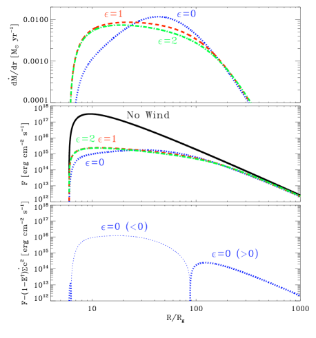
Figure 2: Upper panel: The implied mass-loss rate versus $R$ for models with $\epsilon=0$ (blue, dotted), 1 (red, dashed) and 2 (green, dot-dashed). All models correspond to $M/M_{\odot}=10^{7}$, $a_{*}=0$ and $\dot{m}=2$ at a large radius. Mass loss is modelled using the $\dot{\Sigma}(F)$ prescription. The integrated mass loss decreases as $\epsilon$ increases, with the largest outflow coming from the $\epsilon=0$ model, for which a larger fraction of the outflow occurs at a larger radius. Middle panel: The flux corresponding to the model shown in the upper panel and a model with no outflow (solid black). The larger fraction of energy that is lost in unbinding the flow for larger $\epsilon$ is offset by lower implied outflow rates and the flux profiles for the models with mass loss are all very similar. Bottom panel: The difference between the radiative flux and the energy required to unbind the implied outflow for the model with $\epsilon=0$. The thin dotted curve shows where this quantity is negative. The negative value implies that mass loss is so great that there is insufficient energy to unbind it. Hence, most of the mass lost from the thin disk, if $\epsilon=0$, must ultimately accrete, possibly in the form of a much hotter and geometrically thick flow.

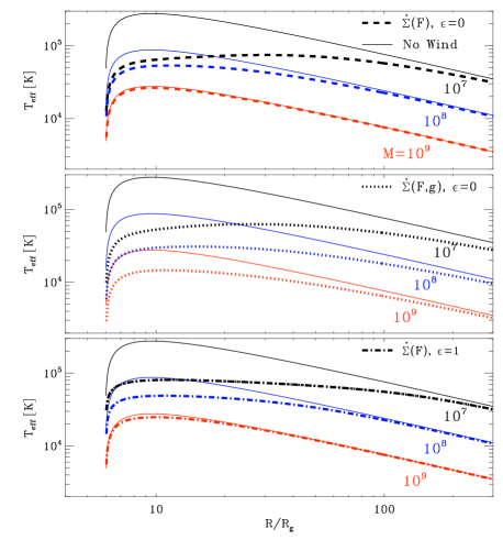
Figure 3: Upper panel: The $T_{\rm eff}$ versus $R$ for models with $M/M_{\odot}=10^{7}$, $10^{8}$, and $10^{9}$. All models correspond to $a_{*}=0$ and $\dot{M_{1}}=0.94$ at a large radius, which corresponds to $\dot{m}=2$, 0.2, and 0.02, respectively. The solid curves are standard AD models with no mass loss while the dashed curves show models with mass loss given by $\dot{\Sigma}(F)$ with $\epsilon=0$. Note the reduced difference in $T_{\rm max}$ between the $M/M_{\odot}=10^{7}$ and $10^{8}$ mass loss models, compared to the standard solution. The AD in the $M/M_{\odot}=10^{9}$ model is too cold to produce significant mass loss, and $T_{\rm eff}$ profile remains the same. Middle panel: Same as the upper panel but the dotted curves correspond to $\dot{\Sigma}(F,g)$ with $\epsilon=0$. This mass loss term yields a weaker $R$ dependence of $\dot{M}$, and thus a more gradual rise at smaller $R$ in the deviation of $T_{\rm eff}$ from the standard solution. Bottom panel: Same as the upper panel, but the dot-dashed curves correspond to $\dot{\Sigma}(F)$ with $\epsilon=1$. In this case the $T_{\rm eff}$ continues to increase very mildly as radius decreases, rather than decreasing slightly as in the $\epsilon=0$ case.

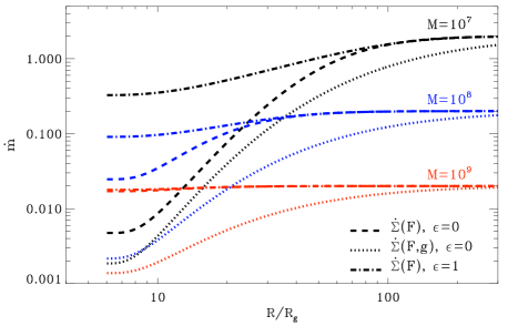
Figure 4: The local $\dot{m}$ versus $R$ for the models shown in Fig. 3. The implied drop in $\dot{m}$ towards $R_{\rm ISCO}$ becomes larger with decreasing $M$, as the AD gets hotter, and can reach a factor of 1000 in the most extreme model, corresponding to $M=10^{7}M_{\odot}$, $\dot{\Sigma}(F,g)$, and $\epsilon=0$. The models with $\epsilon=1$ generically produce less implied mass loss, with most extreme case ($M=10^{7}M_{\odot}$) having $\dot{M}_{\rm out}\sim 6\dot{M}_{\rm in}$. The $M/M_{\odot}=10^{9}$ and $\dot{\Sigma}(F)$ models show no significant mass loss for either value of $\epsilon$.

Figure 3 presents numerical solutions for $T_{\rm eff}(r)$. The results are presented for the two $\dot{\Sigma}$ relations, and for different $M$ values. The top panel presents the $\dot{\Sigma}(F)$, $\epsilon=0$ AD model solution for $T_{\rm eff}(r)$, for $M=10^{7},10^{8},10^{9}M_{\odot}$. All models correspond to $a_{*}=0$ and $\dot{M_{1}}=0.94$ at $r\gg r_{\rm in}$, which corresponds to $\dot{m}=2$, 0.2, and 0.02, respectively. For comparison we also show the corresponding standard SS73 solution for $T_{\rm eff}(r)$ with no mass loss, i.e. a constant $\dot{m}$ ($=\dot{m}(r_{\rm out})$). Note the similar $T_{\rm max}$ in the $M=10^{7}M_{\odot}$ and $10^{8}M_{\odot}$ models, with a ratio of 1.4, in contrast with the ratio of $3.16$ for the SS73 solution (equation 13). The simplified analytic solution ratio (equation 14) of $10^{0.14}=1.38$, is remarkably close to the numerical solution ratio of 1.4. The absolute values of $T_{\rm max}$ in the analytic solution, $7.2\times 10^{4}$ K for $M=10^{7}M_{\odot}$ is also very close to the numerical solution value of $7.5\times 10^{4}$ K. The $M=10^{9}M_{\odot}$ model is cold enough to suppress $\dot{\Sigma}(F)$, so that $\dot{m}_{\rm wind}(r)/\dot{m}\ll 1$, and the solution overlaps the SS73 no wind solution.

The middle panel shows the numerical solution using $\dot{\Sigma}(F,g)$ and $\epsilon=0$ for the same parameters as in the upper panels. The mass loss is more pronounced, and its rise towards the center is more gradual, as expected from the simplified analytic solution (equation 20 vs. equation 11). The wind remains significant also for the $M=10^{9}M_{\odot}$ models. The ratios of $T_{\rm max}$ from the $M=10^{7}M_{\odot}$ and $10^{8}M_{\odot}$ models are, 2.03, somewhat larger than with the $\dot{\Sigma}(F)$ relation.

The bottom panel shows a model with $\dot{\Sigma}(F)$ and $\epsilon=1$. Although the implementation of the outflow differs significantly from the top panel, the thermostatic effect is still apparent. In this case the ratio of $T_{\rm max}$ for the $M=10^{7}M_{\odot}$ and $10^{8}M_{\odot}$ models is 1.65, compared to 1.4 for the $\epsilon=0$ model above, and significantly less than the SS73 model. As above, there is very little mass lost for the $M=10^{9}M_{\odot}$ model. Models with $\dot{\Sigma}(F,g)$ and $\epsilon=1$ (not shown) have $T_{\rm eff}(r)$ profiles qualitatively similar to those with $\dot{\Sigma}(F,g)$ and $\epsilon=0$.

Figure 4 shows the implied $\dot{m}(r)$ profiles for the models in Figure 3. In the simplified analytic solution the disc truncates at $r_{\rm eq}$, where $\dot{m}_{\rm wind}(r_{\rm eq})=\dot{m}(r_{\rm out})$. In the numerical solutions, the drop in $\dot{m}(r)$ towards the center suppresses the rise in $T_{\rm eff}(r)$, and thus reduces a further rise in $\dot{m}_{\rm wind}(r)$ towards the center. This negative feedback prevents $\dot{m}_{\rm wind}(r)$ from ever reaching $\dot{m}(r_{\rm out})$, and the disc always (nominally) extends down to $r_{\rm ISCO}$. However, the implied total mass loss can be very large. The $\dot{\Sigma}(F,g)$ model with $\epsilon=0$ yields $\dot{m}(r_{\rm in})/\dot{m}(r_{\rm out})=0.00092$ for $M=10^{7}M_{\odot}$, and the $\dot{\Sigma}(F)$ model with $\epsilon=0$ yields $\dot{m}(r_{\rm in})/\dot{m}(r_{\rm out})=0.0024$. Thus, although formally the thin disc extends down to $r_{\rm ISCO}$, it effectively terminates at a larger radius in these cases. For example, $\dot{m}(r)/\dot{m}(r_{\rm out})=0.5$ at $r=62$ for the $\dot{\Sigma}(F)$ $M=10^{7}M_{\odot}$ model, and at $r=20$ for the $M=10^{8}M_{\odot}$ model (the simplified analytic solution, equation 12, gives truncation radii of $r=85$ and 28 respectively). Inside these transition radii, the implied $\dot{m}(r)$ profiles should be regarded with suspicion, given a possible feedback of the mass loss on the thin disk solution. Obtaining reliable profiles in this region probably requires a more sophisticated disc model.

The coldest models with $M=10^{9}M_{\odot}$ has no significant mass loss for models employing the $\dot{\Sigma}(F)$ relation. This is consistent with the $T_{\rm eff}(r)$ solution in the upper and lower panels of Figure 3, which matches the no wind SS73 solution, as $\dot{m}(r)$ remains effectively constant. The $\dot{\Sigma}(F,g)$ relation yields a more gradual drop in $\dot{m}(r)$ towards the center for all $M$, but with a significantly larger amplitude, with significant wind also for $M=10^{9}M_{\odot}$.

Figure 5 explores the effect of the black hole spin $a_{*}$ on $T_{\rm eff}(r)$, for the models assuming outflow rates of $\dot{\Sigma}(F)$ and $\epsilon=0$ and 1. The solutions of $T_{\rm eff}(r)$ are presented for $a_{*}=0,0.7,0.9$, All models correspond to $M=10^{8}M_{\odot}$, and $\dot{M_{1}}=0.94$ at large $r$, which corresponds to $\dot{m}=0.2$, 0.36, and 0.54, respectively. The SS73 solutions are also shown for comparison. In contrast with the SS73 solution, where $T_{\rm max}$ rises with $a_{*}$, as $r_{\rm ISCO}$ gets smaller, in the $\epsilon=0$ case all models reach a nearly identical $T_{\rm max}$, which occurs at $r\simeq 10$, well outside the largest $r_{\rm ISCO}=6$. The value of $T_{\rm max}$ is well below the SS73 range of values, as shown above in Figure 3. The AD extension to smaller $r$ with increasing $a_{*}$ just produces an extended inner region with $T\simeq T_{\rm max}$, from $r\simeq 20$ down to $r\simeq r_{\rm ISCO}$. The strong dependence of $\dot{\Sigma}$ on the local $F$ effectively serves as a local thermostat, which prevents $F$ from rising above the limiting $T_{\rm max}$ value. Thus, the wind breaks the tight relation between $T_{\rm max}$ and $a_{*}$, which exists in models with no mass loss.

The $\epsilon=1$ models show a slight rise in $T_{\rm eff}(r)$ towards smaller $r$, but since the emitting area scales as $r^{2}$, we will see that this weak increase has almost no effect on the observed SED.

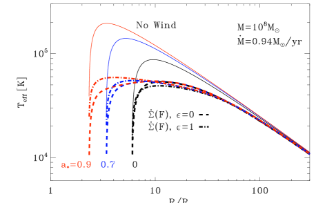
Figure 5: The $T_{\rm eff}(r)$ solution for models with $a_{*}=0$, $0.7$ and $0.9$. All models correspond to $M=10^{8}M_{\odot}$ and have $\dot{M_{1}}=0.94$ at a large radius, which corresponds to $\dot{m}=0.2$, 0.36, and 0.54, respectively. The solid curves denote standard accretion disc (SS73) models with no mass loss. The dashed and dot-dashed curves denote models with mass loss given by $\dot{\Sigma}(F)$ for $\epsilon=0$ and $\epsilon=1$, respectively. In contrast with the SS73 models, all $\epsilon=0$ models reach the same $T_{\rm max}$. This reflects the thermostatic effect of $\dot{\Sigma}$, which sets a cap on $T_{\rm max}$, and produces a nearly isothermal AD at $r\sim 2-20$. For the $\epsilon=1$ models, $T_{\rm eff}$ continues to rise to small $R$, but much more weakly than in the SS73 models. Since the emitting area decreases, these innermost radii contribute little to the disc integrated luminosity. At larger $R$, which dominate the bolometric output, the profiles nearly overlap, as in the $\epsilon=0$ models.

The results presented in Figures 3 and 5 clearly show that $T_{\rm max}$, remains well below $10^{5}$K. There is some dependence of $T_{\rm max}$ on the AD parameters, but the dependence is significantly reduced compared to the solutions with no winds, particularly for the $\dot{\Sigma}(F)$ relations. The numerical solutions are rather close to the simplified analytic estimate made in §3 for $r_{\rm eq}$ and $T_{\rm max}$. The qualitative similarities between the models with $\epsilon=0$ and $\epsilon=1$ suggest the thermostatic effect of the wind could be quite robust. The difference between the $\epsilon=0$ and 1 models is their significantly different $\dot{m}(r)$ in the hottest models. The models utilizing the $\dot{\Sigma}(F,g)$ outflow prescription, generally provide too much outflow, leading to discs considerably colder than those observed.

6 The Derived SED

6.1 The local Blackbody models

Figure 6: The specific luminosity $\lambda L_{\lambda}$ versus $\lambda$ for blackbody emission corresponding to the models with different $\dot{\Sigma}$ and $\epsilon$, as noted in the plot. All models assume no torque at the inner boundary, $a_{*}=0$, $M=10^{8}M_{\odot}$, and $\dot{m}=0.2$ at large $R$. The standard model with no mass loss (solid) peaks at $\lambda\sim 600$Å, significantly shorter than typically observed. The $\dot{\Sigma}(F)$ models peak at $\lambda\sim 1000$Å, as typically observed. The $\dot{\Sigma}(F,g)$ models, characterized by a stronger and more extended mass loss, peaks at $\lambda>2000$Å, colder than typically observed.

We now consider the SED predicted by the disc models in the presence of a mass outflow. The outflow can modify the spectrum in two primary ways: by modifying the underlying thin disc solution, as derived above, and also via its direct emission or reprocessing (absorption and scattering) of radiation from the underlying disc. In this work we focus only on the effects on the underlying thin disc solution, which may produce the universal turnover at $\lambda<1000$Å. A more complete calculation requires modeling the outflow (Murray et al., 1995; Proga et al., 2000) to compute the effect of reprocessed emission (see e.g. Sim et al., 2010) on the SED. Such models require detailed numerical simulations that are beyond the scope of this work.

We first study the derived SED based on the simple local blackbody SED calculations, computed directly from the $T_{\rm eff}(r)$ profiles discussed above. We later present the results from a more detailed model which includes radiative transfer and the vertical structure of the atmosphere. The advantage of the simplified local blackbody calculation is that the results are insensitive to assumptions about the vertical dissipation distribution. We break the disc up into concentric annuli equally spaced in $\log r$. At each radius we compute a blackbody spectrum at $T_{\rm eff}(r)$, weighting by the emitting area of the annulus and summing over all radii yields full disc SEDs. For the sake of simplicity, the effects of relativity on photon propagation are neglected at this stage, and are included in the following more detailed atmospheric calculations.

Figure 6 presents the SED for the outflow prescriptions described in §5.1. We use the $T_{\rm eff}(r)$ profiles presented in Figure 3 for $M=10^{8}M_{\odot}$, $\dot{m}(r_{\rm out})=0.2$, and $a_{*}=0$. The blackbody SED with no outflow peaks at $\sim 600$ Å, too far in the UV to be consistent with the observed SEDs of $10^{8}M_{\odot}$ black holes. The $\epsilon=0$ and 1 $\dot{\Sigma}(F)$ models both yield peaks at $\sim 1000$ Å, as typically observed. The $\dot{\Sigma}(F,g)$ models, which predicts more mass loss, peaks long-ward of $2000$ Å, too long to be consistent with observations of most luminous AGN.

Figure 7 presents the SEDs as a function of $M$. It compares the SEDs derived from the $\dot{\Sigma}(F)$ model for $\epsilon=0$ and $\epsilon=1$ with the standard SS73 SEDs. As expected from the $T_{\rm eff}(r)$ solutions (Figure 2), the $M=10^{7}M_{\odot}$ and $M=10^{8}M_{\odot}$ wind solution SEDs show similar peak wavelengths. For $\epsilon=0$, the wavelength ratio is 1.4 (830Å vs. 1170Å), as expected from their $T_{\rm max}$ ratio of 1.4. The $M=10^{9}M_{\odot}$ SED is nearly identical to the solution with no wind, as expected from the negligible $\dot{M}_{\rm wind}$. The factor of 10 in the $\nu_{\rm peak}$ position (210Å vs. 2130Å) for the local blackbody solution of $M=10^{7}M_{\odot}$ and $M=10^{9}M_{\odot}$ with a fixed $\dot{M}$, is reduced to a factor of $<3$ (830Å vs. 2250Å). At long enough wavelengths ($\lambda>3000$Å) the SED remains unchanged, as the emission originates from outer colder regions in the AD where the wind is negligible.

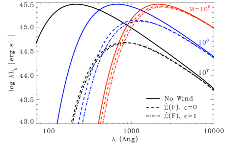
Figure 7: The specific luminosity $\lambda L_{\lambda}$ versus $\lambda$ for blackbody emission corresponding to the models presented in Figure 3 using the $\dot{\Sigma}(F)$ prescription with $\epsilon=0$ (dashed) and $\epsilon=1$ (dot-dashed). The peak emission wavelength decreases with $M$ in all models, but in the models with outflow this sensitivity to $M$ is significantly reduced. With these relations, the $10^{9}M_{\odot}$ models are cold enough to have a negligible wind effect on the SED. The integrated luminosity drops with $M$ when mass loss is included in the models, as expected from the $\dot{m}(r)$ solutions. There are only very modest difference between the $\epsilon=0$ and $\epsilon=1$ models, suggesting the thermostatic effect on the SED is fairly robust.

Similar conclusions hold for the models assuming $\epsilon=1$. In this case the $M=10^{7}M_{\odot}$ and $M=10^{8}M_{\odot}$ models have a peak wavelength ratio of 1.45, which is somewhat less than their $T_{\rm max}$ ratio of 1.65. This difference is a result of the shallow $T_{\rm eff}(r)$ profile in Figure 3. Even though $T_{\rm eff}$ still rises as $R$ declines, the rise is small, and the maximum occurs at smaller radii with lower emitting area, and thus contributes relatively little to the SED. Therefore, the ratio of the peak emission wavelengths is set by somewhat larger radii where the $T_{\rm eff}$ ratio between the two different mass models is smaller. Models with $\dot{\Sigma}(F,g)$ (not shown) are too cold to correspond to the observed SEDs.

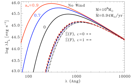
Figure 8: The specific luminosity $\lambda L_{\lambda}$ versus $\lambda$ for blackbody emission corresponding to the models with different $a_{*}$ presented in Figure 5. Even though the SEDs for models without mass loss (solid) vary significantly with $a_{*}$, the models with mass loss are essentially identical. This reflects the thermostatic effect of $\dot{\Sigma}$, which produces a nearly isothermal disc at $r<20$ (see Fig. 5). The SED is thus blind to the value of $a_{*}$.

Figure 8 presents the dependence of the SED on $a_{*}$ based on the models shown in Figure 5. The models with no mass loss show a harder SED with increasing $a_{*}$, as $r_{\rm ISCO}$ gets smaller and the AD reaches a higher $T_{\rm max}$. In sharp contrast, the dependence of the SED on $a_{*}$ disappears completely once $\dot{\Sigma}$ is included. Although the thin AD still extends down to $r_{\rm ISCO}$ (see Fig. 5), this innermost region is not hotter than the outer regions for the $\epsilon=0$ models, due to the thermostatic effect of $\dot{\Sigma}$ on $T_{\rm max}$ mentioned above (§5.1). The models with $\epsilon=1$ have a shallow rise in $T_{\rm eff}$ towards the center, but the small emitting area again means these hotter regions contribute very little to the overall emission. In both cases the contribution to the SED from the $r\sim 2$ region is negligible compared to the contribution of the $r\sim 20$ region. The SED is thus blind to the inner extension of the disc, and therefore to the value of $a_{*}$, for the AD parameters explored in this figure.

6.2 The TLUSTY models

Due to atomic features and electron scattering it is expected that the local SED may differ significantly from blackbody emission (SS73; Kolykhalov & Sunyaev, 1984). Detailed modeling of the disc vertical structure is required to accurately model these departures from blackbody emission (see e.g. Hubeny et al. 2000; 2001). When mass loss is an appreciable fraction of the mass accretion rate, a substantial portion of the disc surface layers can no longer be in hydrostatic equilibrium. In the CAK theory these departures from hydrostatic equilibrium are due to the force multiplier from line opacity. In principle these lines could be modelled directly by a stellar atmospheres code such as TLUSTY, but this would significantly increase the complexity and computational cost of such calculations (e.g. Kudritzki & Puls 2000). Therefore, we approximate the disc emission using hydrostatic models, as used in previous studies with no mass outflow (Hubeny et al., 2000). Although the characteristic peak energy of the SED should be reasonably insensitive to this assumption, the spectrum of emission at shorter wavelengths may be significantly modified.

Even with hydrostatic models, the mass loss has a significant impact on the spectrum through its modification of $F(r)$ and $\Sigma(r)$, as non-blackbody models are generally sensitive to both. We now proceed using the same integration method described in section 5.1, again assuming no torque at the inner boundary. We combine the resulting profiles of $F(r)$ and $\Sigma(r)$ with a radial profile of the vertical gravity, and use the interpolation methods described in Davis & Hubeny (2006) to construct full AD SEDs, accounting for relativistic effects on photon geodesics (Dexter & Agol, 2009). We compute $\Sigma(r)$ using an $\alpha$ relation for the stress and solving an algebraic equation that smoothly transitions between the gas and radiation pressure dominated limits, as described in Appendix B of Zhu et al. (2012). The only difference here is that we compute $F_{1}=W_{R\phi}/\alpha$ using our numerically integrated $W_{R\phi}$ rather than assuming that the last equality in their equation (B3a) holds.

Figure 9 compares the TLUSTY derived SEDs as a function of $M$ for models with and without mass loss. All models have $\dot{M}(r_{\rm out})=0.94\rm M_{\odot}/yr$, $a_{\ast}=0$, $i=40^{\circ}$. Here we only consider one mass loss prescription, using the $\dot{\Sigma}(F)$ relation with $\epsilon=0$ as an example. The TLUSTY based models with no mass loss peak at higher energies compared to the local blackbody models of the same parameters (Fig. 7), due to the larger fraction of the opacity dominated by electron scattering at short wavelengths, and the resulting modified blackbody emission. Absorption edge features are also present. All the models with mass loss are significantly colder, as expected. An interesting new feature is that, in contrast with the local blackbody models, where there is a gradual shift to lower $\nu_{\rm peak}$ with a rising $M$, here all models show a similar peak position near the Lyman edge, and a break in the spectral slope above and below the edge. This occurs because of the jump in absorption opacity across the edge. This spectral break is remarkably similar to the universal break observed at $\lambda\sim 1000$Å in the mean SEDs of AGN (Telfer et al. 2002; Shull et al. 2012). The slope shortward of 1000Å depends on $M$, and the lowest $M=10^{7}M_{\odot}$ model shows that the spectral slope can remain close to $-1$ far into the EUV.

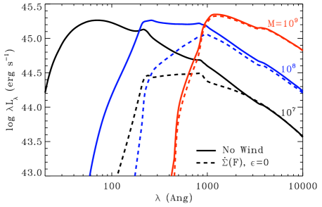
Figure 9: Comparison of the specific luminosity $\lambda L_{\lambda}$ versus $\lambda$ for TLUSTY-based models with (dashed) and without (solid) mass loss for different $M$ values. Mass loss assumes $\dot{\Sigma}(F)$ and $\epsilon=0$, with each model computed to yield $\dot{M}(r_{\rm out})=0.94M_{\odot}/{\rm yr}$. All models account for relativistic effects on photon propagation, and assume an inclination of $40^{\circ}$. The TLUSTY based models are much harder due to modified blackbody effects resulting from significant electron scattering opacity and the presence of strong edge features. All the models with mass loss show a peak and a spectral break near 1000 Å, similar to the universal break at 1000 Å seen in the spectra of AGN. However, the spectral slope at $\lambda<1000$ Å is predicted to be harder at lower $M$ models.

6.3 The derivation of $\dot{M}$

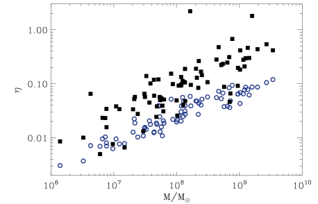
Figure 10: The radiative efficiency $\eta$ versus $M$ for a sample of 80 PG quasars. The black filled squares denote the efficiencies inferred by DL11, assuming a standard disc model with no mass loss to estimate $\dot{M}$. The blue open circles denote the implied efficiencies in models with mass loss given by $\dot{\Sigma}(F)$ for the same $M$ and $\dot{M}$ used in the DL11 analysis. They assume $a_{*}=0.9$. The slope of the correlation implied by the models is qualitatively consistent with the DL11 results, but with a lower mean and reduced variance of $\eta$.

How does the modified AD SED derived here affect the derivation of $\dot{M}$ from the optical luminosity in AGN? In an earlier work (DL11), we provide a useful expression which allows to derive $\dot{M}$ based on the optical luminosity, when $M$ is known, assuming the continuum is produced by a thin AD with no mass loss. As shown above (excluding some implausible very cold AD models produced by the $\dot{\Sigma}(F,g)$ relation), the wind becomes significant only in the hotter UV emitting regions, and thus it has a negligible effect on the optical emission. Thus, the AD based $\dot{M}$ derivation remains valid. This method was applied to the PG sample of quasars to derive the radiative efficiency $\eta\equiv L_{\rm bol}/\dot{M}c^{2}$, which was found to show a clear trend with $M$ of the form $\eta\propto M^{0.5}$ (DL11). This trend can be interpreted as an indication for a trend of a rising $a_{*}$ with $M$. However, as discussed in DL11, the $\eta\propto M^{0.5}$ relation can be derived from the universal SED of AGN, and it was not clear whether the trend of $\eta$ with $M$ just happens to lead by coincidence to a universal SED, or whether the universal SED is a more fundamental property, which leads to an apparent $\eta\propto M^{0.5}$ relation. Now that we have a physical mechanism which may lead to a rather universal SED, we can explore its effect on the $\eta$ versus $M$ relation, and in particular study whether the observed $\eta$ versus $M$ relation has any implication on an $a_{*}$ versus $M$ relation.

Figure 10 presents the $\eta$ vs. $M$ relation derived in DL11 for the PG sample of quasars. We now explore whether a similar relation can be derived if the SED of these objects is produced by an AD with mass loss, using the $\dot{\Sigma}(F)$ relation with $\epsilon=0$, but with a fixed value of $a_{*}$. For each object we construct a local blackbody AD+wind model with the tabulated $M$ in DL11, and a fixed value of $a_{*}=0.9$ for all objects. We iterated over the boundary value of $\dot{M}(r_{\rm in})$ in order to get the tabulated $\dot{M}$ for that object in DL11. We then integrated over the AD luminosity to get the predicted $L_{\rm bol}$, and from that derive the predicted radiative $\eta$, which is plotted in Figure 10. The $\eta$ derived here tends to be lower by a factor of 2-3 from the one measured in DL11, however it shows a rather tight correlation with $M$, of a similar slope to the one derived in DL11. Since the $\eta\propto M^{0.5}$ correlation can result from a universal SED, it is not surprising that the disc+wind model SED used here to derive $L_{\rm bol}$, leads to a similar relation, as this model produces similar SEDs over a wide range of $M$ and $\dot{M}$. This trend can also be understood from the simplified analytic solution (equation 12), which gives $r_{\rm eq}\propto M^{-0.48}$, and the fact that in a thin AD $\eta$ is given by the innermost disc radius. Thus, the observed $\eta$ vs. $M$ relation in DL11 does not necessarily imply an $a_{*}$ vs. $M$ relation, as $\eta$ may be set by $r_{\rm eq}$, which is independent of $a_{*}$.

7 Discussion

The SS73 solution was constructed with stellar-mass black hole systems in mind, which have a much hotter AD than in AGN. As a result, the dominant opacity in stellar systems is electron scattering and free-free absorption. In AGN AD, the maximum temperature drops from $\sim 10^{7}$ to $\sim 10^{5}$K, and UV line opacity becomes the dominant photospheric opacity source. This likely explains why the observed SED in binary black hole systems is well matched by simple thin AD models (Davis et al. 2005; 2006), while in AGN there is generally a gross mismatch between the predicted and observed emission from the innermost part of the AD. Various AGN AD models did take bound-free opacity into account (e.g. Czerny & Elvis 1987; Laor & Netzer 1989; Ross et al. 1992; Storzer 1993; Sincell & Krolik 1997), and also included careful calculations of the vertical structure coupled to the radiative transfer (Hubeny et al. 2000; 2001). However, none of the models included line opacity. In O stars, the line opacity inevitably leads to a wind, and it may have a similar effect in AGN.

Winds are prevalent in AGN, as indicated by the broad and blueshifted resonance line absorption observed in broad absorption line quasars (e.g. Reichard et al. 2003). The winds most likely originate from the AD, and a likely driving mechanism is radiation pressure on resonance lines, as indicated by both analytic solutions (Murray et al. 1995) and numerical calculations (Proga et al. 2000). Here we find that radiation pressure driven winds may modify significantly the disc structure. Applying the mass loss per unit area measured in O stars, we find that the simple thin disc solution effectively terminates at a few tens of $R_{g}$. The steep dependence of the local mass loss on $T_{\rm eff}$, $\dot{\Sigma}(F)\propto T_{\rm eff}^{7.6}$ (equation 2) sets a cap on the maximum $T_{\rm eff}$, which is well below $10^{5}$K. This can explain why the observed AGN SEDs do not show a rise towards the EUV, and may also explain the rather universal turnover observed at $\lambda<1000$Å.

The softening effect of an AD wind mass loss on the SED of AGN was noted by Witt et al. (1997) and Slone & Netzer (2012), and for cataclysmic variables by Knigge (1999). The new result here is the application of the stellar mass loss to AGN AD, which yields a UV turnover similar to the one observed, with no free parameters. In contrast with Slone & Netzer (2012) and Knigge (1999), where general $\dot{M}_{\rm wind}(r)$ relations were assumed, here we find that the derived $\dot{M}_{\rm wind}(r)$ relation which matched the observed SED, has a negligible effect on the derived $\dot{M}(r_{\rm out})$ (DL11), as there is negligible wind at the region where the optical emission is produced. However, it is certainly correct that $\dot{M}(r_{\rm in})$ may be significantly smaller than $\dot{M}(r_{\rm out})$ , as was pointed out by DL11 and Slone & Netzer (2012).

Lawrence (2012) proposed that obscuration near, but external to the accretion disc, produces the nearly constant SED peak. Obscuring material off the plane of the disc but at low radius is assumed to be provided by outflows from (or instabilities in) the disc. This model assumes that mass lost to obscuring clouds is not large enough to modify the intrinsic disc emission, which is instead altered by transfer through the obscuring clouds. Although we have not computed the effects of reprocessing by the outflow, such reprocessing likely occurs and the effects described in Lawrence (2012) may be present at some level.

7.1 Are O stars winds applicable to AGN?

The CAK wind solution applies for spherically symmetric systems, where both gravity and the radiation field fall off as $1/r^{2}$. In AD there are significant differences. Thin AD are rotationally supported, and in the local disc frame, close to the disc surface, gravity increases linearly with height, while the radiation field is independent of height. Thus, it is not clear that the CAK solution is relevant even locally close to the surface of the AD. Far enough above the disc, where $h>r$, both gravity and the radiation field become radial and fall off as $1/r^{2}$. Thus, in contrast with the stellar case, in AD both the relative strength and directions of the radiative and gravitational forces change with position. Proga, Stone & Kallman (2000) find that as a result there is no steady state solution, in contrast with the steady state stellar wind solution.

A related issue is the difference in the velocity fields in AD and in O stars. AD are expected to have Keplerian velocity shear and be highly turbulent. Since line driven wind models from O stars generally assume monotonically increasing velocity profiles, non-monotonic velocity distributions (due e.g. to the turbulence) may modify the acceleration of the outflow. Modeling such effects requires fairly sophisticated radiative transfer calculations beyond the scope of this work, which to the best of our knowledge have not been considered elsewhere.

In addition, the integrated SED in AGN is harder than in stars, and thus the wind is subject to over-ionization once it becomes exposed to the harder EUV - soft X-ray radiation, which may shut off line driving if the ionization is large enough. Previous studies (e.g. Murray et al. 1995) have generally assumed that such irradiation only becomes important after the matter has been lifted significantly above the disc surface. However, if the inner region of the disc is thick enough it may directly irradiate the disc at larger radii, increase the ionization level and reduce the force multiplier at the disc surface. Such direct irradiation is not expected in the radiation dominated regions of a SS73 solution because the AD scale height is nearly constant with radius. In any case, the irradiating flux falls off a $r^{-3}$ and likely remains a small fraction of the locally dissipated flux (Blaes 2004). Significant flaring of the disc or scattering of radiation by the failed wind might increase the irradiation, enhancing the ionization level at the disc surface and potentially inhibiting the outflow. For the line driven wind to be a viable explanation of the ‘universal’ UV break, the outflow clearly cannot be completely quenched.

The local force multiplier within an unirradiated disc atmosphere is likely similar to that in an atmosphere of a star with the same $T_{\rm eff}$. The force multiplier is $\Gamma\sim 10^{3}$ (Lamers & Cassinelli 1999) at a column of $\sim 10^{18}\;\rm cm^{-1}$ from the disc surface, which inevitably leads to a modification of the disc vertical structure. The SS73 solution assumes only electron scattering, leading to a thin disc with a height $h<r$ for $\dot{m}<1$. An increase in the opacity, i.e. $\Gamma>1$, will expand the disc atmosphere vertically, and can lead to a disc thickness $h^{\prime}\sim\Gamma h$. For $\Gamma>r/h$ the disc atmosphere becomes geometrically thick. If $h^{\prime}>r$ then $g\propto 1/r^{2}$, a hydrostatic solution is not possible anymore, and a wind is launched. Since $r/h\sim 10-100$ typically in thin discs, a $\Gamma\sim 10^{3}$ should lead to a wind. However, once the wind is exposed to the central ionizing continuum, it may get significantly ionized (depending on its density), leading to $\Gamma\la 10$ (Murray et al. 1995, Fig.9 there). An acceleration length of $\sim r/\Gamma$ will bring the wind to the escape velocity, and allow it to escape, even if it gets over ionized at the coasting phase. If the outflow does not attain the escape speed before being over ionized, the gas will fall back to the disc, forming a ‘failed wind’.

Proga et al. (2000) present a model for a UV line driven wind from an AD with $m_{8}=1,\dot{m}=0.5$. They find a time averaged $\dot{M}_{\rm wind}/\dot{M}=28$%, for $\dot{M}_{\rm wind}$ measured at $r>200$. This wind is shielded by the failed wind produced close to the inner boundary of the simulation (at $r=150$), which is over-ionized by the central X-ray source. The AGN AD wind simulation of Proga & Kallman (2002) show a sharp rise in the local mass loss at $r<100$ (fig.1 there), and thus the integrated $\dot{M}_{\rm wind}$ lifted from the surface may reach $\dot{M}_{\rm wind}/\dot{M}\sim 1$ closer to the center, as derived by our simplistic use of the CAK solution. As noted by Proga (2005) this line driving can change the vertical structure of the disc, and likely produce a “puffed up” disc.

7.2 What happens in the innermost disc?

In section 5, we considered two sets of models which can have rather different implications for mass loss from the disc. Models in which the work done in unbinding the outflow is negligible ($\epsilon=0$) can nominally drive almost all of the matter out of the thin disc. However, the energy required to drive all this material to escape velocity can exceed the energy released by the remaining disc material which accretes to the center (e.g. the $10^{7}M_{\odot}$ models with $\dot{m}_{\rm out}=2$, see Fig.3). Hence, there must be a substantial failed wind in this scenario and most of the material in this failed wind must eventually accrete, although possibly not in the form of a standard, thin disc.

In the second set of models with $\epsilon=1$, we account for the energy lost by radiation in unbinding the outflow to compute $F$ and use this to evaluate the $\dot{\Sigma}$ relations. In this case the mass loss is limited by the corresponding reduction in $F$. The mass outflow rate can still be quite large ($\sim 90$ % of $\dot{M}$ at large radius), but the accreted mass is significantly larger relative to the $\epsilon=0$ models. All the energy needed to accelerate the outflow to escape velocity is accounted for and there is no need for a failed wind to form a hotter, radiatively inefficient flow.

Although the latter models have the appeal of being explicitly energy conserving, the numerical simulations discussed above (e.g. Proga et al. 2000) suggest winds may not operate in this fashion. They are predominately accelerated by the radiation from annuli interior to their launching radius, so the assumption of a constant $\epsilon$ is likely a poor approximation. More importantly, the winds behave (in certain respects) more like the $\epsilon=0$ models, in that they launch more matter from the thin disc than they accelerate to infinity and forming a “failed wind.” These simulations assume a constant $\dot{M}$ AD as a boundary condition, and find outflow rates as high as 50% of this prescribed $\dot{M}$. In principle, even higher outflow rates could be obtained, but such models have not been considered due to the assumed lack of feedback on the boundary condition in the models used (D. Proga, private communication).

Our best guess is that a real system would behave like some combination of the above models: a significant fraction of the radiative flux will go into accelerating some fraction of the outflow that does exceed escape velocity and becomes a wind, but not all of the mass removed from the thin disc will become unbound. Much of it may form a failed wind that returns to the disc or accretes through a hotter, geometrically thick flow.

The distinction between the thin disc and the outflow probably breaks down when a non-negligible fraction of the disc is no longer in hydrostatic equilibrium. Since the calculations presented in section 5 do not account for the detailed vertical structure, the radial distributions of $T_{\rm eff}$ and $\dot{M}$ in regions where $\dot{M}_{\rm wind}(r)\sim\dot{M}(r_{\rm out})$ should be interpreted with this in mind. If most of the material lifted from the disc falls back, say due to over ionization, then it must eventually all accrete to the center. In this case, observations would seem to require a hot, radiatively inefficient flow, since substantial thermal EUV emission is not seen. The bulk of “fallback” flow must remain hotter and thicker than standard solution, cooling primarily via inverse-Compton scattering and contributing significant radiation only in the X-ray band. In this scenario, line-driving would result in a transition from a thin, radiatively efficient disc to a geometrically thick, radiatively inefficient flow.

A low radiative efficiency can occur in hot flows if the optical depth is very low or very high (see e.g. Narayan & Yi, 1994, 1995; Abramowicz et al., 1988, 1995). When the optical depth is large, the radiation is advected inwards inside a thick disc, when the radiation diffusion time-scale is longer than the infall time-scale. This effect is expected to be present in discs with $\dot{m}>1$, where the AD becomes slim, rather than thin (Abramowicz et al., 1988). Interestingly, all objects in DL11 with an observed radiative efficiency below 2% have measured $\dot{M}$ which corresponds to an AD with $\dot{m}\sim 3-30$ for a 10% efficiency. So, advection of radiation may indeed suppress the emission from the innermost disc. However, the SED of such a high $\dot{m}$ disc typically peaks well shortward 1000Å, so it is inconsistent with the observed $\lambda\sim 1000$Å turnover. Another process is responsible for the universal $\lambda\sim 1000$Å turnover.

The unbound material in the inner AD must remain hot enough to avoid emitting significantly in the observable UV band. What is the expected emission from this hot inner region? Can it form the thick and hot inner structure often invoked as a source for the X-ray emission? Let us assume the X-ray emission is produced in the inner AD region through comptonization of the incident thin disc emission which comes from $r>r_{\rm eq}$, where the thin disc resides. The Compton cooling takes place only in a $\tau_{\rm es}\sim 1$ surface layer of the illuminated hot and thick configuration at $r<r_{\rm eq}$. So, only a small fraction of the inner disc volume will cool radiatively, while the rest of the dissipated energy should be advected inwards. The estimated X-ray luminosity of this surface layer can be derived based on the thermal energy stored in this layer divided by the cooling time. The likely projected surface area of the inner hot disc is $A=cos(\theta)2\pi r^{2}$, where $r\sim r_{\rm eq}$ (equation 12), and $cos(\theta)\sim 0.1$ is the illumination angle of the external radiation, which yields $A=1.6\times 10^{29}m_{8}^{1.04}\dot{M_{1}}^{0.48}$ cm². The illuminated column density corresponds to $\tau_{\rm es}\sim 1$. The electron temperature is $T\sim 10^{9}$K (from the spectral slope of $-1$ for comptonization, Rybicki & Lightman 1979, equation 7.45b). Thus, the total thermal energy of the electrons in the illuminated layer is $E=A\Sigma kT=5\times 10^{46}m_{8}^{1.04}\dot{M_{1}}^{0.48}$ erg. The Compton cooling time of electrons embedded in a blackbody at $T=10^{5}T_{5}$ is $t_{C}=81.5T_{5}^{-4}$ s (e.g. Laor & Behar 2008, equation 53). Approximating the disc emission as a blackbody at $T_{\rm max}$ (equation 14), gives a cooling rate of the illuminated layer of $E/t_{C}=L_{X}\sim 10^{44}\dot{M_{1}}^{0.76}m_{8}^{0.48}$. How does it compare with the bolometric luminosity? The expected $L_{\rm bol}$ from the geometrically thin AD, which extends down to $r_{\rm eq}$, is $\sim\dot{M}c^{2}/r_{\rm eq}$, or $L_{\rm bol}\sim 10^{45}\dot{M_{1}}^{0.76}m_{8}^{0.48}$. We thus get $L_{X}\sim 0.1L_{\rm bol}$, which is close to the typical ratio observed in AGN.

To summarize, the radius of the inner thick disc, the assumption it is maintained at $T\sim 10^{9}$K by the viscous dissipation, the implied Compton cooling time based on the incident radiation from the thin AD, and the thermal energy content of the cooling surface layer of the inner hot disc, happen to combine together and give a constant $L_{X}/L_{\rm bol}$, of the order of magnitude observed.

If the inner X-ray source is produced by a breakdown of the thin disc solution due to line opacity driving, while the X-ray source is significant enough to quench the disc wind, this may lead to an instability in the X-ray and EUV emission, and an anticorrelation between the two bands. The inner AD may switch back and forth from a thermal EUV emitting thin AD state, which develops a strong wind and turns into a thick and hot X-ray emitting configuration, which shuts off the wind, and turns back to the thin thermal EUV emission state, which again develops a strong wind.

7.3 What happens at lower Masses?

With decreasing $M$ the disc gets hotter, the wind starts at a larger $r$ (eqs.12, 21), and the radiative efficiency is expected to get lower (see also $\eta\propto M^{0.5}$, DL11). This may partly explain why accreting $M\leq 10^{6}M_{\odot}$ systems are rare. A wind launched at a larger $r$ may find it easier to escape, and low $M$ black holes may find it harder to grow by accretion. However, at a low enough $M$, $r_{\rm eq}$ will move out into the gas pressure dominated regime of the disc. In this regime the disc is vertically supported by the gas pressure, so an increase in radiation pressure due to $\Gamma>1$ does not necessarily lead to a significant change in the vertical structure. A values of $\Gamma>10^{3}$ close to the disc surface will most likely overcome gravity and drive a wind. However, in contrast with the uniform vertical density profile of the radiation dominated part of the disc, in the gas dominated part the density drops steeply with height, and thus the density at the sonic point, which feeds the base of the wind may be significantly lower, lowering $\dot{M}_{\rm wind}$.

Another effect which comes in with decreasing $M$ is that $T_{\rm max}$ increases, reaching $>2\times 10^{5}$ K for $M=10M_{\odot}$ (eqs. 15, 23). At this temperature $\Gamma$ likely decreases due to over-ionization of the primary atomic UV absorbers, which will also reduce $\dot{M}_{\rm wind}$.

Observations of Cataclysmic Variables (CV) which harbour AD around white dwarfs, yield winds with $\dot{M}_{\rm wind}<<\dot{M}$ (e.g. Feldmeier et al. 1999), despite the fact that the CV AD peaks in the UV. However, these systems are characterized by $\dot{M_{1}}\sim 10^{-8}$, $m_{8}\sim 10^{-8}$, and $r_{\rm in}\sim 10^{4}$. Plugging these values into equation (11) gives $\dot{M}_{\rm wind}/\dot{M}\sim 10^{-2}$, which is likely an overestimate as the AD in CV is gas pressure rather than radiation pressure dominated. Thus, CV AD have only weak winds, despite their peak UV emission and the associated high $\Gamma$ values, due to their large $r_{\rm in}$ (see equation 11).

In X-ray binaries (XRB) systems, the disc is much more compact, reaching $T\sim 10^{7}$ K. Therefore, the gas becomes fully ionized and line opacity is negligible. If the outer disc extends far out enough, it can reach the $\Gamma\gg 1$ regime, this time from the other side of the opacity barrier, probably at $T<10^{6}$ K, where the line opacity starts to build up, which may also produce a wind, this time from the outer disc, rather than the inner disc. The wind is expected to move inwards in the low hard state, as the disc gets cooler, which may disrupt the thin disc formation down to the center.

For an $M<10^{6}M_{\odot}$ black hole radiating near Eddington, the inner regions of a SS73 disc reach $T>10^{6}$ K, and should emit predominantly in the soft X-rays (Done et al., 2012). At this temperature the ionization may be high enough to reduce $\Lambda$ and allow a thin disc solution with no wind. Further out the disc will be colder, and significant mass loss is likely to occur, which may strongly suppress $\dot{M}$ which can arrive to the center. However, if a fraction of $L_{\rm bol}$, which peaks at soft X-rays, is intercepted farther out in the disc, wind launching may be quenched further outside. Such a scenario may explain some low mass ($M<10^{6}M_{\odot}$) narrow line Seyfert 1s with large soft X-ray “excesses”, such as RE J1034+396 (Done et al., 2012).

7.4 Can $a_{*}$ be measured from the SED and the Fe K$\alpha$ line?

Since the line driven wind effectively terminates the thin disc well outside $r_{\rm ISCO}$, the value of $a_{*}$ does not affect the thin disc SED. Thus, in contrast with XRB, we generally do not expect the AGN SED to provide a useful constraint on $a_{*}$. However, for a sufficiently cold disc, with a turnover at $\lambda>1000$Å, the wind disappears. This may explain the remarkably good fit of a simple local BB AD model to SDSS J094533.99+100950.1, (Czerny et al. 2011; Laor & Davis 2011), which is a weak line quasar with a UV turnover at $\lambda\sim 2000$Å (Hryniewicz et al. 2010). We therefore expect that other cold AD quasars, i.e. quasars with a blue SED at $\lambda>3000$Å (which excludes dust reddening), and a UV turnover at $\lambda>1000$Å, can also be well fit by a simple local BB AD model. One may therefore be able to constrain $a_{*}$ based on the SED in these quasars, as commonly done now in XRB (e.g. Li et al. 2005; Shafee et al. 2006; McClintock et al. 2011)).

Similar issues may apply to efforts to measure $a_{*}$ via models of the Fe K$\alpha$ line and ionized reflection. The numerical solutions indicate that an optically thick disc extends down to $r_{\rm ISCO}$. However unless the disc is cold, only a small fraction of $\dot{M}$ extends down to $r_{\rm ISCO}$. The numerical solution ignores the material which left the thin disc, which may form a thick configuration in which the thin disc is embedded, if it exists at all. A lack of a thin cold bare disc which extends down to $r_{\rm ISCO}$ will affect the expected profile of the fluorescence Fe K$\alpha$ line, produced by X-ray reflection from the AD. The line may be dominated by emission outside $r_{\rm eq}$, which will make the line narrower, and its profile independent of the value of $a_{*}$. Line emission inside $r_{\rm eq}$ will depend on the gas temperature, and the line profile may be modified by possible scattering effects at a thick and hot surface layer. In any case, the emission is not expected to originate from a thin bare AD, as commonly assumed, as a thin bare disc which extends down to $r_{\rm ISCO}$ is simply not observed. We do predict that the colder the disc is, the further it extends inwards, and the broader the K$\alpha$ line can be.

7.5 What is the effect on the characteristic half-light radius?

The outflow changes the radial distribution of the emitted flux in different frequency bands. In particular, the reduction of the far UV emission relative to the SS73 solution leads to an increase in the half-light radius for the optical to UV bands. This is because the Rayleigh-Jeans tail of the emission from the UV peaked regions of the disc contributes a non-negligible fraction to the overall SED at longer wavelengths. Removing this emission or shifting it to X-ray wavelengths increases the fraction of the long wavelength emission from larger radii.

This effect is interesting in light of claims based on microlensing analysis of lensed quasars that the optical to UV emission comes from radii which are factors of $\sim 3-10$ larger than expected from the standard thin disc model (e.g. Mortonson et al., 2005; Pooley et al., 2007; Morgan et al., 2010). However, the increases in the half-light radius (which the microlensing results are claimed to measure) that we infer are typically $<30\%$ at 2000 Å and $<10\%$ at 4000 Å relative to the models with no outflow, so this effect cannot account for the large discrepancies that are claimed. A caveat is that we have not considered the reprocessing of the thin disc emission by the outflow. For such large mass loss rates the wind will likely be optically thick to Thomson scattering in the radial direction (Sim et al., 2010). Some fraction of this will be scattered downward and be reprocessed by the disc at larger radii. This reprocessed emission should increase the half-light radius at longer wavelengths, although a more detailed calculation is required to estimate the possible magnitude of the effect.

7.6 Predictions

The inwards extent of the AD can be probed through the position of the UV turnover. The $\dot{\Sigma}(F)$ wind relation generally predicts a turnover at $\lambda_{\rm peak}\sim 1000$Å. However there is still some residual dependence on $\dot{m}$ and $m_{8}$, possibly in the form of $T_{\rm max}\propto(\dot{m}/m_{8})^{0.07}$ (equation 15), which should be observationally detectable. The quantity $\dot{m}/m_{8}$ can be estimated based on the broad emission lines, which gives $M=v_{\rm BLR}^{2}R_{\rm BLR}/G$, where the H$\beta$ FWHM is used to derive $v_{\rm BLR}$. In addition, $R_{\rm BLR}\propto L^{0.5}$ based on reverberation mappings, and the above relations imply $\dot{m}/m_{8}\propto v_{\rm BLR}^{4}$. Thus, the $\dot{\Sigma}(F)$ wind relation (equation 15) implies that $T_{\rm max}\propto v_{\rm BLR}^{0.28}$, or $\lambda_{\rm peak}\propto v_{\rm BLR}^{-0.28}$. A factor of 10 increase in $v_{\rm BLR}$ will therefore be associated with a decrease by factor of 2 in $\lambda_{\rm peak}$. This is true as long as the disc is not too cold to become windless, i.e. when $v_{\rm BLR}$ is not too large ($\la 10,000$ km s^-1, e.g. Laor & Davis 2011). In general, the detection of a correlation of $\lambda_{\rm peak}$ with $\dot{m}$ and $m_{8}$ can provide a hint on the specific form of $\dot{\Sigma}$ in AGN AD.

A clear prediction is a metallicity dependence of $\lambda_{\rm peak}$. Radiation driven wind models for hot stars predict a close to linear relation of $Z$ and $\dot{M}$ (e.g. Abbott 1982; Leitherer et al. 1992; Vink et al. 2001; Kudritzki 2002). Since $r_{\rm eq}\propto\dot{M}_{\rm wind}^{0.27}$ for the $\dot{\Sigma}(F)$ wind relation, and in AD $T_{\rm max}\propto r^{-3/4}$, we expect that $\lambda_{\rm peak}\propto Z^{-0.2}$. Although the expected dependence of $\lambda_{\rm peak}$ on $Z$ is weak, it is a robust prediction of line driven winds, and its detection will provide strong support for the wind interpretation put forward in this paper.

8 Conclusions

We derive the Navier-Stokes equations for gas on circular orbits in a thin AD, including local mass loss and angular momentum loss terms. We then solve these equations numerically for a Keplerian disc, with zero torque inner boundary condition. We apply the local mass loss terms per unit area measured in hot stars, as a function of $F$ and $g$, at the AD surface. We assume no angular momentum loss induced by the mass loss. We calculate the derived SED based on the local blackbody approximation, and also using the TLUSTY stellar atmosphere code. We find the following.

1. Line driven winds put a cap on the AD $T_{\rm max}<10^{5}K$, with a weak dependence on $M$ and $\dot{m}$. This cap is consistent with observation of AGN SEDs, which generally show a spectral turnover near 1000Å.

2. In most cases the thin AD is effectively truncated at a few tens $R_{g}$, well outside $r_{\rm ISCO}$. The derived SED is thus independent of the value of $r_{\rm ISCO}$, and is therefore independent of the value of $a_{*}$.

3. In a cold AD, defined by an SED with a turnover longward of 1000Å, the line driven wind is negligible. It may therefore be possible to use the SED of objects predicted to have a cold AD, based on their measured $M$ and $\dot{m}$, to derive the black hole $a_{*}$.

4. The TLUSTY based models with winds tend to show a spectral break at $\lambda\sim 1000$Å, due to a combination of the Lyman edge and the truncation of the hot inner part of the AD due to the wind.

5. Depending on the mass loss prescription, $M$, and $\dot{m}$ of the model, the material removed from the thin disc either escapes as a wind or forms a failed wind that must accrete. In either case, the thin disc solution of SS73 cannot generally extend to $r_{\rm ISCO}$, as the emission from the inner region of a thin disc is generally not observed.

6. For a sufficiently large failed wind, the inner disc must be radiatively inefficient. It may form a geometrically thick hot inflow. If the electron temperature can be maintained at $T\sim 10^{9}$ K, then Compton cooling leads to $L_{X}\sim 0.1L_{\rm bol}$.

7. The $\dot{\Sigma}(F)$ wind relation implies a radiative efficiency which scales as $M^{0.5}$, which agrees with the measured relation (DL11). Thus, the low radiative efficiency of low $M$ AGN does not imply a low $a_{*}$, but may be induced by high mass loss and the implied large truncation radius of the inner thin AD.

8. If the UV turnover is indeed a line driven mass loss effect, then the effect is necessarily $Z$ dependent. Higher $Z$ object should show a larger $\lambda_{\rm peak}$, i.e. a softer ionizing SED at a given $M$ and $\dot{M}$.

Rather detailed wind simulations are available, and it will be interesting to explore the radiation transfer through the wind/failed wind, and its possible impact on the observed SED. However, a major uncertainty in wind models remains concerning the vertical structure of the disc, in particular the top layer from which the wind is launched. The structure depends on the exact nature of the turbulence and how it is dissipated. Thus, one cannot yet derive estimates for $\dot{M}_{\rm wind}(r)$ from first principles. We went around this major uncertainty by adopting $\dot{M}_{\rm wind}(r)$ derived based on $\dot{M}_{\rm wind}(g,T_{\rm eff})$ of O stars. Although the models adopted here are rather simplified, they yield SEDs remarkably similar to those generally observed, without significant sensitivity to the details of the launching mechanism. However, the structure of the innermost disc and its possible feedback, in particular when the implied outflow becomes comparable to the accretion rate, need to be further explored.

One possible feedback is X-ray irradiation of the innermost disc, which if strong enough, may ionize the surface disc layer to a level which will quench the line driven wind. If the hot inner disc is indeed formed by a line driven failed wind, then quenching the wind may quench the X-ray source, which will allow the wind to form again.

Despite the associated uncertainty in the above analysis, a plausible statement one can make is that in AGN, as in O stars, “a static atmosphere is not possible” (CAK, §II there). The true structure of the inner AD remains to be understood.

Appendix A Relativistic Accretion Discs with Outflow

In section 4.1, we derive the equations of conservation of mass, angular momentum, and energy in the Newtonian limit. Here describe the fully relativistic generalizations to these equations The derivation of the relativistic equations for the steady state, axisymmetric disc without mass loss has been discussed extensively in previous work (see e.g. Novikov & Thorne, 1973; Page & Thorne, 1974; Riffert & Herold, 1995). Here we generalize these derivations to include the effect of an outflow. These works differ in the formulation of the eqs. of hydrostatic equilibrium, but all agree on the appropriate thin disc limit of the equations for conservation of mass, angular momentum and energy. These correspond to eqs. (4), (9), and (16) in Riffert & Herold (1995). Specifically, they are conservation of mass

$$(\rho U^{\alpha})_{;\alpha}=0,$$ (35)

conservation of energy

$$S^{\alpha\beta}U_{\alpha;\beta}+q^{\beta}_{~{};\beta}=0,$$ (36)

and conservation of angular momentum

$$\rho U^{\beta}U^{\phi}_{~{};\beta}+S^{\phi\beta}_{~{}~{};\beta}+U^{\phi}U_{\alpha}S^{\alpha\beta}_{~{}~{};\beta}=0.$$ (37)

Here $U^{\alpha}$ is the four-velocity, $\rho$ is the rest mass density, $S^{\alpha\beta}$ is the stress tensor and $q^{\alpha}$ is radiative energy flux.

Now we integrate the steady state equations over $z$, initially neglecting any energy loss associated with unbinding of the outflow. As above, $F_{M}$ represent the flux of mass out of the thin disc. Conservation of mass is identical to the Newtonian version (equation 24). Conservation of angular momentum and energy become

$$\frac{\partial}{\partial r}\left(\dot{M}L^{\dagger}-2\pi rW_{r}^{~{}\phi}\right)=4\pi rL^{\dagger}(Q+F_{M})$$ (38)

$$\frac{\partial}{\partial r}\left(\dot{M}E^{\dagger}-2\pi rW_{r}^{~{}\phi}\Omega\right)=4\pi rE^{\dagger}(Q+F_{M}).$$ (39)

We have adopted the notation of Page & Thorne (1974), where $L^{\dagger}$ and $E^{\dagger}$ denote the energy and specific angular momentum at infinity, $W_{r}^{~{}\phi}$ is the vertical integral of the $r$–$\phi$ component of the viscous stress tensor, and $\Omega$ is the rotation rate of a circular orbit. Here, $Q$ represents the (“viscous”) dissipation associated with stresses in the accretion flow. (In a model with no outflow, it corresponds to the flux emitted from the disc surface.) In analogy with equation (26) we define the radiative flux observed at infinity as

$$F=E^{\dagger}Q-\epsilon F_{M}(1-E^{\dagger}).$$ (40)

where

$$E^{\dagger}=\frac{1-2/r+a_{*}/r^{3/2}}{\left(1-3/r+2a/r^{3/2}\right)^{1/2}}$$ (41)

Using this expression and defining $dL/dr=4\pi rF$, equation (39) can be integrated from $r_{\rm in}$ to infinity to find

$$L=\dot{M}_{\rm in}(1-E^{\dagger}_{\rm in})-(\epsilon-1)\int^{\infty}_{r_{\rm in}}\frac{\partial\dot{M}}{\partial r}(1-E^{\dagger})dr.$$ (42)

Here $\dot{M}_{\rm in}$ and $E^{\dagger}_{\rm in}$ are evaluated at $r_{\rm in}$, where we have assumed that the internal torque vanishes. Hence the total luminosity radiated by the disc (as observed at infinity) is just the standard disc efficiency using the mass accretion rate at the inner edge minus the work done accelerating the flow beyond its escape velocity (if $\epsilon>1$).

For our numerical solution, it is useful to rewrite the equations in terms of the co-moving frame quantities $W_{r\phi}$ and the Keplerian rotation $\Omega_{K}$. Equation (38) becomes

$$\frac{\partial W_{R\phi}}{\partial R}+\frac{2(R-R_{g})}{R^{2}A_{\rm RH}}W_{R\phi}=\frac{\dot{M}\Omega_{K}}{4\pi R}\frac{E_{\rm RH}}{A_{\rm RH}B_{\rm RH}},$$ (43)

and equation (39) becomes

$$Q=-\frac{3}{4}W_{R\phi}\Omega_{K}\frac{A_{\rm RH}}{B_{\rm RH}}.$$ (44)

$A_{\rm RH}$, $B_{\rm RH}$, and $E_{\rm RH}$ are functions of $r$ and $a_{*}$ defined in Riffert & Herold (1995) that approach unity for large $r$. These are identical to eqs. (14) and (17) of Riffert & Herold (1995), and in the limit that $R\gg R_{g}$, they reduce to eqs. (26) and (28).

References

- Abbott (1982) Abbott, D. C. 1982, ApJ, 259, 282
- Abramowicz et al. (1988) Abramowicz, M. A., Czerny, B., Lasota, J. P., & Szuszkiewicz, E. 1988, ApJ, 332, 646
- Abramowicz et al. (1995) Abramowicz, M. A., Chen, X., Kato, S., Lasota, J.-P., & Regev, O. 1995, ApJ, 438, L37
- Balbus & Hawley (1998) Balbus, S. A., & Hawley, J. F. 1998, Reviews of Modern Physics, 70, 1
- Balbus & Papaloizou (1999) Balbus, S. A., & Papaloizou, J. C. B. 1999, ApJ, 521, 650
- Barger & Cowie (2010) Barger, A. J., & Cowie, L. L. 2010, ApJ, 718, 1235
- Blaes (2004) Blaes, O. M. 2004, Accretion Discs, Jets and High Energy Phenomena in Astrophysics, 137
- Bonning et al. (2013) Bonning, E. W., Shields, G. A., Stevens, A. C., & Salviander, S. 2013, ApJ, 770, 30
- Castor et al. (1975) Castor, J. I., Abbott, D. C., & Klein, R. I. 1975, ApJ, 195, 157. (CAK)
- Czerny & Elvis (1987) Czerny, B., & Elvis, M. 1987, ApJ, 321, 305
- Czerny et al. (2011) Czerny, B., Hryniewicz, K., Nikołajuk, M., & Sa̧dowski, A. 2011, MNRAS, 415, 2942
- Davis et al. (2005) Davis, S. W., Blaes, O. M., Hubeny, I., & Turner, N. J. 2005, ApJ, 621, 372
- Davis & Hubeny (2006) Davis, S. W., & Hubeny, I. 2006, ApJS, 164, 530
- Davis et al. (2006) Davis, S. W., Done, C., & Blaes, O. M. 2006, ApJ, 647, 525
- Davis & Laor (2011) Davis, S. W., & Laor, A. 2011, ApJ, 728, 98 (DL11)
- Dexter & Agol (2009) Dexter, J., & Agol, E. 2009, ApJ, 696, 1616
- Done et al. (2012) Done, C., Davis, S. W., Jin, C., Blaes, O., & Ward, M. 2012, MNRAS, 420, 1848
- Feldmeier et al. (1999) Feldmeier, A., Shlosman, I., & Vitello, P. 1999, ApJ, 526, 357
- Howarth & Prinja (1989) Howarth, I. D., & Prinja, R. K. 1989, ApJS, 69, 527
- Hubeny & Lanz (1995) Hubeny, I., & Lanz, T. 1995, ApJ, 439, 875
- Hubeny et al. (2000) Hubeny, I., Agol, E., Blaes, O., & Krolik, J. H. 2000, ApJ, 533, 710
- Hubeny et al. (2001) Hubeny, I., Blaes, O., Krolik, J. H., & Agol, E. 2001, ApJ, 559, 680
- Hryniewicz et al. (2010) Hryniewicz, K., Czerny, B., Nikołajuk, M., & Kuraszkiewicz, J. 2010, MNRAS, 404, 2028
- Knigge (1999) Knigge, C. 1999, MNRAS, 309, 409
- Kolykhalov & Sunyaev (1984) Kolykhalov, P. I., & Sunyaev, R. A. 1984, Advances in Space Research, 3, 249
- Kudritzki & Puls (2000) Kudritzki, R.-P., & Puls, J. 2000, ARA&A, 38, 613
- Kudritzki (2002) Kudritzki, R. P. 2002, ApJ, 577, 389
- Lamers & Cassinelli (1999) Lamers, H. J. G. L. M., & Cassinelli, J. P. 1999, Introduction to Stellar Winds, by Henny J. G. L. M. Lamers and Joseph P. Cassinelli, pp. 452. ISBN 0521593980. Cambridge, UK: Cambridge University Press, June 1999.,
- Laor et al. (1997) Laor, A., Fiore, F., Elvis, M., Wilkes, B. J., & McDowell, J. C. 1997, ApJ, 477, 93
- Laor & Behar (2008) Laor, A., & Behar, E. 2008, MNRAS, 390, 847
- Laor & Davis (2011) Laor, A., & Davis, S. W. 2011, MNRAS, 417, 681
- Laor & Netzer (1989) Laor, A., & Netzer, H. 1989, MNRAS, 238, 897
- Lawrence (2012) Lawrence, A. 2012, MNRAS, 423, 451
- Leitherer et al. (1992) Leitherer, C., Robert, C., & Drissen, L. 1992, ApJ, 401, 596
- Li et al. (2005) Li, L.-X., Zimmerman, E. R., Narayan, R., & McClintock, J. E. 2005, ApJS, 157, 335
- Lucy (2010) Lucy, L. B. 2010, A&A, 524, A41
- Malkan (1983) Malkan, M. A. 1983, ApJ, 268, 582
- Malkan & Sargent (1982) Malkan, M. A., & Sargent, W. L. W. 1982, ApJ, 254, 22
- McClintock et al. (2011) McClintock, J. E., Narayan, R., Davis, S. W., et al. 2011, Classical and Quantum Gravity, 28, 114009
- Morgan et al. (2010) Morgan, C. W., Kochanek, C. S., Morgan, N. D., & Falco, E. E. 2010, ApJ, 712, 1129
- Mortonson et al. (2005) Mortonson, M. J., Schechter, P. L., & Wambsganss, J. 2005, ApJ, 628, 594
- Murray et al. (1995) Murray, N., Chiang, J., Grossman, S. A., & Voit, G. M. 1995, ApJ, 451, 498
- Narayan & Yi (1994) Narayan, R., & Yi, I. 1994, ApJL, 428, L13
- Narayan & Yi (1995) Narayan, R., & Yi, I. 1995, ApJ, 444, 231
- Novikov & Thorne (1973) Novikov, I. D., & Thorne, K. S. 1973, in De Witt C. ed. Black Holes (Les Astres Occlus), Gordon and Breach, New York, 346
- Page & Thorne (1974) Page, D. N., & Thorne, K. S. 1974, ApJ, 191, 499
- Pooley et al. (2007) Pooley, D., Blackburne, J. A., Rappaport, S., & Schechter, P. L. 2007, ApJ, 661, 19
- Proga (2005) Proga, D. 2005, ApJ, 630, L9
- Proga et al. (2000) Proga, D., Stone, J. M., & Kallman, T. R. 2000, ApJ, 543, 686
- Proga & Kallman (2004) Proga, D., & Kallman, T. R. 2004, ApJ, 616, 688
- Reichard et al. (2003) Reichard, T. A., Richards, G. T., Schneider, D. P., et al. 2003, AJ, 125, 1711
- Riffert & Herold (1995) Riffert, H., & Herold, H. 1995, ApJ, 450, 508
- Ross et al. (1992) Ross, R. R., Fabian, A. C., & Mineshige, S. 1992, MNRAS, 258, 189
- Rybicki & Lightman (1979) Rybicki, G. B., & Lightman, A. P. 1979, New York, Wiley-Interscience, 1979. 393 p.,
- Scott et al. (2004) Scott, J. E., Kriss, G. A., Brotherton, M., et al. 2004, ApJ, 615, 135
- Shafee et al. (2006) Shafee, R., McClintock, J. E., Narayan, R., et al. 2006, ApJ, 636, L113
- Shakura & Sunyaev (1973) Shakura, N. I., & Sunyaev, R. A. 1973, A&A, 24, 337
- Shakura & Sunyaev (1976) Shakura, N. I., & Sunyaev, R. A. 1976, MNRAS, 175, 613
- Shang et al. (2005) Shang, Z., Brotherton, M. S., Green, R. F., et al. 2005, ApJ, 619, 41
- Shields (1978) Shields, G. A. 1978, Nature, 272, 706
- Shull et al. (2012) Shull, J. M., Stevans, M., & Danforth, C. W. 2012, ApJ, 752, 162
- Sim et al. (2010) Sim, S. A., Proga, D., Miller, L., Long, K. S., & Turner, T. J. 2010, MNRAS, 408, 1396
- Sincell & Krolik (1997) Sincell, M. W., & Krolik, J. H. 1997, ApJ, 476, 605
- Slone & Netzer (2012) Slone, O., & Netzer, H. 2012, MNRAS, 426, 656
- Storzer (1993) Storzer, H. 1993, A&A, 271, 25
- Telfer et al. (2002) Telfer, R. C., Zheng, W., Kriss, G. A., & Davidsen, A. F. 2002, ApJ, 565, 773
- Witt et al. (1997) Witt, H. J., Czerny, B., & Zycki, P. T. 1997, MNRAS, 286, 848
- Vink et al. (2000) Vink, J. S., de Koter, A., & Lamers, H. J. G. L. M. 2000, A&A, 362, 295
- Vink et al. (2001) Vink, J. S., de Koter, A., & Lamers, H. J. G. L. M. 2001, A&A, 369, 574
- Zheng et al. (1997) Zheng, W., Kriss, G. A., Telfer, R. C., Grimes, J. P., & Davidsen, A. F. 1997, ApJ, 475, 469
- Zhu et al. (2012) Zhu, Y., Davis, S. W., Narayan, R., et al. 2012, MNRAS, 424, 2504