The MICE Grand Challenge Lightcone Simulation III:
Galaxy lensing mocks from all-sky lensing maps
Abstract
In paper I of this series (Fosalba et al. 2015), we presented a new N-body lightcone simulation from the MICE collaboration, the MICE Grand Challenge (MICE-GC), containing about 70 billion dark-matter particles in a comoving volume, from which we built halo and galaxy catalogues using a Halo Occupation Distribution and Halo Abundance Matching technique, as presented in the companion Paper II (Crocce et al. 2015). Given its large volume and fine mass resolution, the MICE-GC simulation also allows an accurate modeling of the lensing observables from upcoming wide and deep galaxy surveys. In the last paper of this series (Paper III), we describe the construction of all-sky lensing maps, following the “Onion Universe” approach (Fosalba et al. 2008), and discuss their properties in the lightcone up to with sub-arcmin spatial resolution. By comparing the convergence power spectrum in the MICE-GC to lower mass-resolution (i.e., particle mass ) simulations, we find that resolution effects are at the 5 level for multipoles and 20 for . Resolution effects have a much lower impact on our simulation, as shown by comparing the MICE-GC to recent numerical fits by Takahashi et al 2012. We use the all-sky lensing maps to model galaxy lensing properties, such as the convergence, shear, and lensed magnitudes and positions, and validate them thoroughly using galaxy shear auto and cross-correlations in harmonic and configuration space. Our results show that the galaxy lensing mocks here presented can be used to accurately model lensing observables down to arc-minute scales. Accompanying this series of papers, we make a first public data release of the MICE-GC galaxy mock, the MICECAT v1.0, through a dedicated web-portal for the MICE simulations: http://cosmohub.pic.es, to help developing and exploiting the new generation of astronomical surveys.
1 Introduction
Thanks to the new generation of large astronomical surveys, we have entered in the era of precision cosmology. The high quality data that will be collected by upcoming galaxy surveys, such as DES111www.darkenergysurvey.org, HSC222www.naoj.org/Projects/HSC, Euclid333www.euclid-ec.org, DESI444desi.lbl.gov, HETDEX555hetdex.org, LSST666www.lsst.org, WFIRST777wfirst.gsfc.nasa.gov,etc. will allow to characterize in great detail the distribution of galaxies from the largest accessible scales where linear theory applies down to very small scales described by the non-linear regime of gravitational clustering. Combining observables to beat down probe-specific systematics has the potential to maximize the scientific return of these surveys (Albrecht, 2006; Albrecht & Bernstein, 2007). In particular, traditional probes such as galaxy clustering and cluster abundance can be uniquely complemented with weak lensing data to break degeneracies in cosmological parameters (Weinberg et al., 2013). State-of-the-art weak-lensing observational results have been obtained by the CFHTLenS survey888www.cfhtlens.org (see Kilbinger (2013) and references therein), and build upon previous observations over the last to decades, as summarized in recent reviews (Bartelmann & Schneider, 2001; Van Waerbeke & Mellier, 2003; Hoekstra & Jain, 2008; Bartelmann, 2010).
The ultimate goal of this new generation of surveys is to constrain the nature of dark-energy as well as pin down possible deviations from the standard model, described by General Relativity (Weinberg et al., 2013). But in order to achieve these goals, it is critical to match such experimental efforts with theoretical ones to help developing the science case of these surveys as well as optimally exploiting these large and complex observational datasets.
Theoretical modeling of weak-lensing observables is challenging because the lensing correlations on sub-degree angular scales are described by the non-linear regime of gravitational clustering, where a purely analytic description is not possible. In the absence of a compelling analytic description, Nbody numerical simulations can be used to accurately model the growth of large-scale structures in the non-linear regime and the lensing distortions they produce. Numerical simulations of the weak gravitational lensing are typically based on ray-tracing techniques through Nbody simulations (Blandford et al., 1991; Wambsganss et al., 1998; Jain et al., 2000; White & Hu, 2000; Hamana et al., 2002; Vale & White, 2003; White & Vale, 2004; Hilbert et al., 2009; Becker, 2013). In the ray-tracing approach, light rays are back-traced from the observer to the source, as they are deflected from multiple (typically few tens) of projected-mass lens planes. Measurements of the lensing second and higher-order moments in ray-tracing simulations have been shown to be in good agreement with non-linear theory predictions of gravitational clustering (see e.g., (Gaztanaga & Bernardeau, 1998; Van Waerbeke et al., 2001)).
However, in order to model lensing observables accurately one needs to cover a wide dynamical range: from the large linear (few degree) scales where the power of the deflection field peaks, down to the small (few arcmin) scales that capture the non-linear growth of structures and their associated non-Gaussian contribution to the lensing covariances (Semboloni et al., 2007; Sato et al., 2009; Harnois-Déraps et al., 2012). On the other hand, modeling lensing observables with ray-tracing techniques over a significant portion of the sky are prohibitive in terms of CPU time and memory requirements, and this method is typically restricted to small (few sq.deg.) patches of the sky.
Alternative methods, where the Nbody matter is projected along unperturbed paths using the single-plane (or Born) approximation, have been successfully implemented over large-volume high-resolution simulations to model weak gravitational lensing on curved skies (Gaztanaga & Bernardeau, 1998; Fosalba et al., 2008; Das & Bode, 2008; Teyssier et al., 2009). This novel technique can be readily used to accurately model weak-lensing in wide field galaxy surveys (for sources at ) or the CMB lensing (for ).999In fact Das & Bode (2008) generalize this approach to the multiple-plane case, in the context of CMB lensing, to go beyond the Born approximation
In Paper I of this series (Fosalba et al., 2015) we presented a new N-body simulation developed by the MICE collaboration at the Marenostrum supercomputer, the MICE Grand Challenge run (MICE-GC), that includes about 70 billion dark-matter particles, in a box of about aside. This simulation samples 5 orders of magnitude in dynamical range, covering from the largest (linear) scales accesible to the observable universe where clustering statistics are Gaussian, down to to the highly non-linear regime of structure formation where gravity drives dark-matter and galaxy clustering away from Gaussianity. Using the MICE-GC dark-matter outputs in the lightcone, we built a mock galaxy catalog using a hybrid Halo Occupation Distribution and Halo Abundance Matching (HOD+HAM) technique, whose galaxy clustering properties were discussed in detail in Paper II (Crocce et al., 2015).
In the last paper of the series (Paper III) we describe the construction of all-sky lensing maps, with sub-arcmin resolution and discuss their application to model galaxy lensing properties, such as the convergence, shear, and lensed magnitudes and positions of the synthetic HOD+HAM galaxy catalog.
Following up on the analyses presented in the previous papers of this series, one of the main focus of this work is to investigate the impact of mass-resolution effects in the modeling of dark-matter and galaxy clustering observables by comparing the MICE-GC, and previous MICE runs, to analytic fits available based on high-resolution N-body simulations. For this purpose, we have used the “Onion Universe” approach (Fosalba et al., 2008) to build lensing observables from pixelized 2D maps of the dark-matter in the lightcone. Starting from the convergence, we derive other observables including the shear, deflection and lensed positions and magnitudes. We have then developed several tests to validate this observables using basic lensing statistics, such as the convergence and shear angular power spectrum and the shear 2-point correlation functions, and the cross-correlations of foreground and background galaxy samples to extract the magnification signal. Our analysis shows that the all-sky lensing maps and galaxy lensing properties derived from them can be used to model upcoming galaxy surveys with high accuracy from the largest (linear) scales down to the small ( arcmin) scales described by the non-linear regime of gravitational clustering.
This paper is organized as follows: §2 briefly describes the MICE-GC run and its parameters. In §3 we describe the construction of all-sky maps of lensing observable such as convergence, shear and the deflection field, from the dark-matter outputs in the lightcone, and in §4 we show how we assign lensing properties to the mock galaxies, and validate our implementation by using 2-point shear auto and cross-correlation statistics in harmonic and configuration space. We also present a novel application of our all-sky lensing maps: the modeling of magnification in mock galaxy positions and magnitudes is discussed in §5 Finally, in §6 we summarize our main results and conclusions.
2 The MICE Grand Challenge Simulation
In Paper I of this series (Fosalba et al., 2015), we presented and validated a new large volume cosmological simulation, the MICE 101010further details about the MICE project can be found here www.ice.cat/mice Grand Challenge simulation (MICE-GC hereafter), developed at the Marenostrum supercomputer at BSC 111111Barcelona Supercomputing Center, www.bsc.es, using the public Nbody code Gadget2 (Springel, 2005). The MICE-GC simulation contains dark-matter particles in a box-size of (i.e., samples a cosmological volume of ), and the softening length used is, . Therefore this simulation covers a very wide dynamic range, close to five orders of magnitude in scale, with a good mass resolution, .
In Table 1 we describe the Gadget-2 code parameters used in the MICE simulations discussed in this paper: the MICE Grand-Challenge (MICE-GC), the Intermediate Resolution (MICE-IR; Fosalba et al. (2008)) and the Super-Hubble Volume (MICE-SHV; Crocce et al. (2010)). Further details about the MICE-GC run and the validation of its dark-matter outputs using various 3D and 2D clustering statistics are given in Paper I (Fosalba et al., 2015).
| Run | |||||||||
|---|---|---|---|---|---|---|---|---|---|
| MICE-GC | |||||||||
| MICE-IR | |||||||||
| MICE-SHV |
3 All-sky Lensing maps
Following the approach presented in Fosalba et al. (2008), construct a lightcone simulation by replicating the simulation box (and translating it) around the observer. Given the large box-size used for the MICE-GC simulation, , this approach allows us to build all-sky lensing outputs with negligible repetition up to . Then we decompose the dark-matter lightcone into a set of all-sky concentric spherical shells, of given width , around the observer, what we call the “onion universe”. Each dark-matter “onion shell” is then projected onto a 2D pixelized map using the Healpix tessellation121212http://sourceforge.net/projects/healpix(Górski et al., 2005). For the lensing maps presented in this paper we have chosen a shell-width of megayears in look-back time, which corresponds to a redshift width, , and an angular resolution of Nside arcmin, for the Healpix map resolution Nside that we use. We note that this angular resolution is always larger than the angle subtended by the softening length used for the MICE-GC run, , at the redshifts of interest to derive our lensing observables. In particular, even for the lowest redshift sources, say at , arcmin, and therefore the convolution of the softening length with top-hat pixel window function smooths the gravity force up to angular scales arcmin, within the pixel scale used131313Note that if we use maps with the Healpix resolution Nside, that correspond to a pixel scale of arcmin, we expect the gravitational softening used in the MICE-GC simulation to affect up to arcmin at z=0.5, and therefore the lensing observables will be affected by the softening length effects for lens contributions at redshifts, .
Using these redshift and angular resolutions, we can decompose the lightcone volume in the range into 265 onion shells, each containing Nside pixels. With this set of pixelized lensing maps we construct a finely gridded lightcone output, containing (number of z-bins) pixels (i.e, 3D Gigapixels) with comoving volume, . Total pixelized data volume, using single precision, is about GB. This represents a data compression factor of with respect to the original TB of lightcone output, and thus allows for a much more efficient post-processing analysis.
By combining the dark-matter “onion shells” that make up the lightcone, we can easily derive lensing observables, as explained in Fosalba et al. (2008). This approach, based on approximating the observables by a discrete sum of 2D dark-matter density maps multiplied by the appropriate lensing weights, agrees with the much more complex and CPU time consuming ray-tracing technique within the Born approximation, i.e., in the limit where lensing deflections are calculated using unperturbed light paths
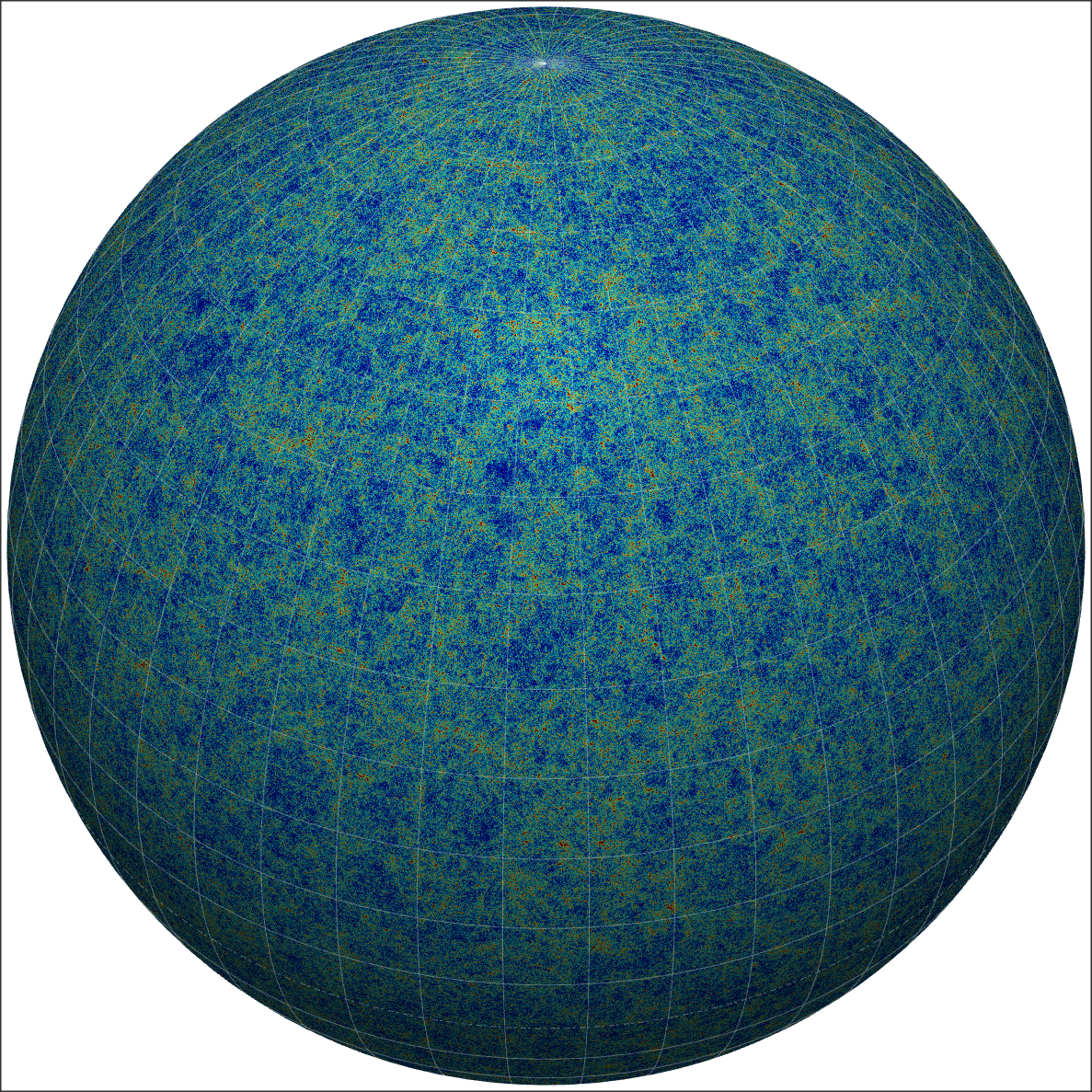
Following this technique we are able to produce all-sky maps of the convergence field, as well as maps for other lensing fields obtained from covariant derivatives of the lensing potential, such as the deflection angle, convergence, shear, flexion, etc. Figure 1 shows the all-sky map of the convergence field, , for the MICE-GC simulation, for sources at , with a pixel resolution of arcmin (i.e., Healpix resolution parameter Nside=4096), produced with the CMBview software141414 https://code.google.com/p/cmbview. The sphere is gridded in sq.deg patches. The color scale shown spans over the range , where is the rms fluctuation of the all-sky convergence map, illustrating the richness in the lensing structures resolved.
In the all-sky limit, we can take the spherical transform of the lensing potential to obtain other lensing observables through simple relations (see Hu (2000)). In the same way it happens with Fourier transforms in the flat-sky limit, spatial derivatives in real space translate into simple multiplications by the corresponding wavenumber (or multipole for curved sky) in the transformed space, as explained in more detail below.
3.1 Convergence
In what follows we shall compute the convergence field for lensing distortions over unperturbed paths, the so-called Born approximation,
| (1) |
where km/s/Mpc is the Hubble constant, is the speed of light, is the 3D matter overdensity at radial distance (for a corresponding scale factor ), and angular position , and is the distance to the lensing sources151515We have assumed flat space, to be consistent with the cosmology used for the MICE-GC run, but this can be trivially generalized for non-flat spaces. Using the “Onion Universe” approach, we can build a pixelized 2D map of the convergence field in the Born approximation by simply adding up the dark-matter “onion shells” or projected density maps in the lightcone, weighted by the weak-lensing efficiency at each redshift,
| (2) |
where indicates a pixel position in the sky and a radial bin (at distance of width ) into which we have sliced the simulation (for further details see Fosalba et al. (2008)).
Using Eq.(1) one gets for the angular power spectrum of the convergence field in the Born approximation,
| (3) |
where is the 3D density power spectrum in the simulation at redshift (corresponding to the radial coordinate in the integral). For the non-linear theoretical predictions, we shall replace above with the numerical fits, such as the Halo model fit to numerical simulations, Halofit (Smith et al., 2003), or the revised Halofit (Takahashi et al., 2012), as implemented in CAMB sources code161616http://camb.info/sources/.
In turn, the convergence field, , is related to the lensing potential through the 2D equivalent to the usual (3D) Poisson equation,
| (4) |
where is the lensing potential at a given point on the celestial sphere, denoted by . The coefficients of the spherical harmonic transform, are given by,
| (5) |
One can thus use this expression to derive the lensing potential at each source plane (or 2D lightcone map), and obtain other lensing observables through their relation to the lensing potential in harmonic space.
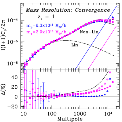
Figure 2 shows the angular power spectrum of the convergence map, , or more precisely, , the contribution to the convergence field variance, , per logarithmic interval in wavenumber , for sources at . The agreement between the Halofit predictions and simulations is within for MICE-IR, and for MICE-GC, down to the resolution scale of the maps used, which corresponds to a multipole Nside 171717We use the Healpix anafast routine, with ring weights, to compute spherical transforms, which are in principle accurate within few percent up to Nside (see http://healpix.sourceforge.net/html/facilities.htm. However we take a conservative approach and only include multipoles up to = 2 Nside in our analysis.. The excess of power we find in the MICE-GC convergence maps with respect to the Halofit is in quantitative agreement with a similar analysis (although limited to a small patch of the sky) performed over the Millennium Simulation (see Fig.9 in Hilbert et al. (2009)), which has more than one order of magnitude lower particle mass (i.e., ).
Comparing the power measured in MICE-GC to that of MICE-IR, we conclude that mass resolution effects are at the 5 level for and 20 for , what is consistent with what was observed for the dark-matter clustering in 2D at the peak of the weak lensing efficiency, i.e., (see Fig.7 of Paper I,(Fosalba et al., 2015)). In turn, the recent “revised” Halofit prediction (Takahashi et al., 2012), based on suite of smaller box realizations, shows a comparable power excess with respect to MICE-GC, what seems to indicate that our simulation might still suffer from mass resolution effects. However, the discrepancy found could be partially due to the difference in box size used between our simulation and the higher-resolution runs by Takahashi et al. (2012). A more complete (and consistent) analysis of mass resolution effects in lensing observables and its possible correlation with other simulation parameters is left for future work.
3.2 Deflection Angle
The gradient of the lensing potential gives the deflection angle, Hu (2000),
| (6) |
and the coefficients of its spherical harmonic transform read,
| (7) |
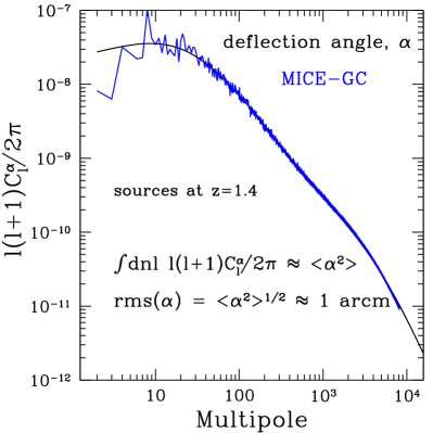
so that the corresponding power spectra are simply related, . Figure 3 shows a comparison between the power spectrum measured in the MICE simulation and the non-linear theoretical fit (i.e., Halofit, see solid line), for sources at . Simulation power spectrum agrees very well with Halofit at all scales. At the lowest multipoles sample variance introduces large fluctuations in the measured power for a single realization. The square root of the integral under the curve gives the rms fluctuation of the deflection field, arcmin.
3.3 Shear
In turn shear maps, , can be simply obtained by decomposing all-sky lensing maps in spherical harmonics (see Hu (2000)):
| (8) |
with, . Assuming that, for the cosmological weak-lensing signal, the B-mode is zero, the shear E-mode harmonic coefficients read, , whereas the ) ”Stokes ” parameters of the shear field,
| (9) |
are then obtained transforming back the ’s to real space.
Fig.4 shows the angular power spectrum for the convergence (black lines) and shear amplitude (blue) for dark-matter at source redshift, in the MICE-GC simulation (wiggly lines), as compared to non-linear theory predictions given by Halofit (smooth lines). The shot-noise contribution (bottom magenta straight line) has been subtracted from the power measured in the simulation. Very good agreement is found between non-linear theory and simulations for a wide dynamical range, similar to what was found for the deflection angle.
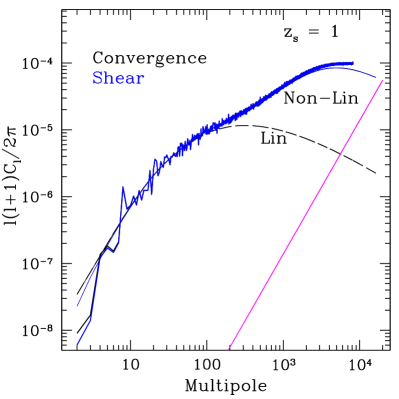
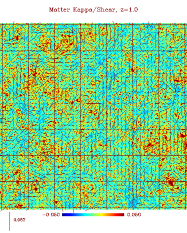
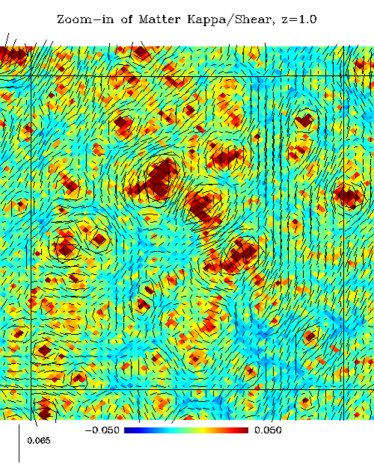
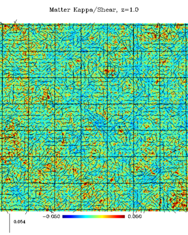
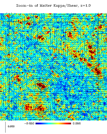
Figure 5 shows 7x7 sq.deg patch of a lensing map from the MICE-GC (top panels) and MICE-IR (bottom panels) simulations. The rectangular grid overplot has a side-length of deg. The amplitude of the convergence field, , is shown color coded, whereas the shear field is shown with vectors on top of the convergence amplitude. As expected in the weak-lensing regime, where the B-mode vanishes, shear vectors are tangential to the projected over-densities (red spots), and point towards under-dense (blue) regions. In the flat-sky limit, in Eq.(8), so that the shear amplitude is given by the convergence field, modulus a global sign. This theoretical expectation is in agreement with simulation measurements, as shown in Figure 4, where both power spectra converge beyond the lowest multipoles (; see wiggly blue and black lines).
The relative lack of resolved small-mass halos in MICE-IR (see e.g, bottom panels in Figure 5 ) with respect to the higher-resolution MICE-GC (top panels) is clearly reflected in the corresponding lower level of well-resolved substructure in the shear maps. This is consistent with the larger amplitude of the projected dark-matter and convergence power spectra for MICE-GC relative to MICE-IR on the smallest scales (i.e., largest multipoles), as seen in Figure 2. One can derive at what scales this mass resolution effect should be visible: the smallest halos resolved in MICE-GC have a mass (corresponding to 10 FoF particle halos), which is roughly the particle mass for MICE-IR. Therefore, according to the halo model for dark-matter clustering, the difference in power between our high and low mass resolution simulations should be due to the 1-halo term contribution from halos with mass , not found in MICE-IR. For the concordance LCDM cosmology adopted these halos have a size 2 Mpc/h and subtend an angle of arcmin ( arcmin) for (), what projects onto multipoles (). This is consistent with what we measured in terms of mass-resolution effects for the dark-matter clustering in Paper I (see Fosalba et al. (2015)): we found MICE-GC has at least larger power than MICE-IR on those scales.
Qualitatively this resolution effect is also observed in the top panels of Figure 5 that shows the lensing map for sources at , that receives a peak contribution from lensing halos at half the distance between the source and the observer, i.e., . As argued above, at this redshift, sources with which project onto an angular size arcmin (i.e, few pixel-sized structures, for the angular resolution of the maps shown), are far more abundant than in the corresponding lensing map for MICE-IR (see bottom panels of Figure 5).
In fact, the magnitude of this effect is expected to increase with redshift for the simple argument that low-mass halos have a relatively larger abundance at high-redshift, as expected from hierarchical clustering, and quantified by the evolution of the halo mass function shape with redshift (see Fig.2 in Paper II, Crocce et al. (2015)). Note this is also consistent with our simulation results for the 3D matter power spectra, as shown in Fig.5 of Paper I (Fosalba et al., 2015), where we obtained a factor of larger mass resolution impact for sources at with respect to those at , on small (non-linear) scales.
4 Galaxy Lensing
Next we turn to our implementation of lensing properties of mock galaxies using the all-sky lensing maps discussed in §3. Mock galaxies are assigned using a hybrid halo occupation distribution and abundance matching (HOD+HAM) approach, as discussed in detail in Paper II (Crocce et al., 2015). In the implementation used for the galaxy mocks discussed in this series of papers, i.e., the MICECAT v1.0, our procedure is a simple 3-step algorithm:
-
1.
for a given galaxy at the 3D position in the lightcone , where gives its angular position in the sky and its redshift, find the corresponding 3D pixel in the discretized lightcone, with pixel center coordinates, , where the galaxy sits in (i.e., the 3D pixel in the suite of “onion slices” or all-sky lensing maps in Healpix tessellation described in §3)
-
2.
get the lensing values for this 3D pixel using the dark-matter all-sky lensing maps, , where the components of the lensing vector are (i.e., convergence and shear), and
-
3.
assign these pixelized dark-matter lensing values, , to the mock galaxy.
This simple implementation of galaxy lensing is limited by the pixel resolution used, Healpix , which corresponds to a pixel scale of arcmin. Consistently, we only expect to model lensing observables accurately down to arcmin scales, as we will discuss in detail below. Another obvious limitation intrinsic to this method is that different galaxies that fall within a given 3D pixel in the “Onion Universe” decomposition of the lightcone, will have identical lensing properties. These two limitations can be overcome using the same approach but using a finer pixel scale (i.e., higher Nside) and/or using interpolation schemes for signals on the sphere (see e.g., Lavaux & Wandelt (2010)). We plan to incorporate these more accurate implementation in future releases of the MICECAT galaxy mocks.
4.1 Converge autocorrelation
In this section we shall validate the implementation of mock galaxy lensing properties introduced in the previous section, by comparing measured 2-point correlation statistics to non-linear theory predictions. We start by focusing on harmonic space and the angular power spectra of lensing observables. For this purpose, we shall use the standard Gaussian approximation to theoretical errors, which includes sample variance and shot-noise contributions (see Kaiser (1992); Stebbins (1996); Crocce et al. (2011)). In this approximation we get for the variance,
| (10) |
where is the cross-spectra between z-bins and , of the foreground and background lensing observables, respectively, and is the shot-noise contribution. For incomplete sky coverage, the effective reduction in independent modes available to a given multipole is accounted by the fraction of the sky factor, . In the case , we recover the variance for the auto-power spectra.
For the convergence power spectra error-bars, we use the theory ’s as given by Eq.(3) and the shot-noise contribution is obtained by integrating the 3D Poisson shot-noise power of the lightcone simulation dark-matter counts at each redshift slice, weighted by the weak-lensing efficiency (i.e., replacing , being the 3D dark-matter counts number density, in Eq.(3) above). The Gaussian approximation is expected to be accurate on large scales and for close to all-sky surveys (see e.g., Cabré et al. (2007)), but they tend to underestimate errors on small-scales, where non-linear gravitational growth induce non-Gaussian covariances through the matter trispectrum (Scoccimarro et al., 1999; Cooray & Hu, 2001). However projection effects inherent to lensing observables mitigate the non-Gaussian contribution relative to the corresponding term in 3D clustering statistics (Semboloni et al., 2007; Takada & Jain, 2009; Hilbert et al., 2009). Given that we only have one single realization in our analysis, the MICE-GC run, we shall stick to the Gaussian approximation for the errors shown in this paper (unless otherwise stated) when comparing to theory predictions, although with the obvious caveat that they tend to underestimate covariances on small-scales. More accurate analysis of weak lensing observables using multiple realizations is left for future work.
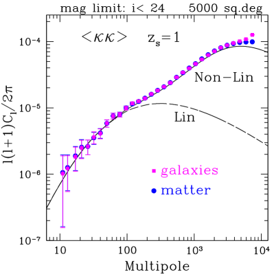
Figure 6 shows the angular power spectrum of the convergence field measured from the MICE-GC simulation for sources at . The galaxy convergence field is expected to be independent of galaxy bias, as it directly traces the underlying (projected) dark-matter distribution. This is in fact what we observe by comparing the convergence for a mock source galaxy sample selected with a magnitude limit in the i band, (see square symbols in plot), and that of the underlying dark-matter density field (circles). Theoretical errors shown are for 5000 sq.deg, which is the area of the sky of the full galaxy mock, MICECAT v1.0, that that we are making publicly available.
4.2 Converge cross-correlation
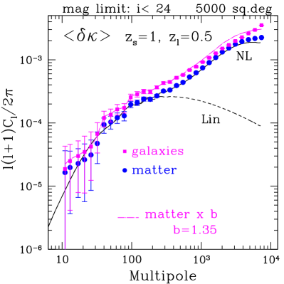
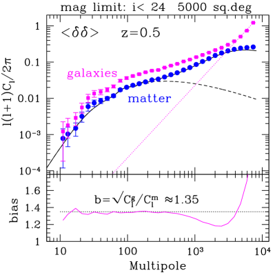
On the other hand, the cross-correlation between background and foreground galaxy populations depends on the bias of the foreground (lens) population. Figure 7 shows that the cross-power measured for source galaxies at with and lenses at (and z-bin widths of for both sources and lenses), see filled circles, is consistent with that for dark-matter scaled by a galaxy bias factor (shown by the dot-dashed line). This is in agreement with the bias estimate from the galaxy auto-power, as shown in the lower panel of Fig.9.

Fig.8 shows the corresponding measurement in configuration space, i.e. the angular cross-correlation:
| (11) |
where correspond to the lenses and to the sources. We count all pairs of galaxies between the two redshift bins and average in angular bins the product of number density fluctuations (counts) and the fluctuations. We also use so that the bias at is .181818Note that at the MICE sample is only complete to , see Fig.5 in paper II. The measurements agree quite well with the non-linear DM prediction (continuous line). On the smallest scales the MICE galaxies show some excess power, which can be interpreted as non-linear bias (similar to that also shown in Fig. 7 at the largest multipoles). Note than on scales smaller that arcmin we expect the MICE measurements to become flat because this is within the healpix pixel radius in the maps. This corresponds to Kpc/h for (see top label in the figure), where the non-linear DM prediction also flattens down and the MICE simulations approaches the softening lengths of Kpc/h. We conclude from this that the resolution of the maps is adequate to model weak lensing to sub arcminute scales. Errors in Fig 8 are obtained from 10 patches of 400 sq.deg.
4.3 Shear correlation functions
Next we validate the shear implemented in MICE dark-matter outputs and galaxy mocks by computing shear correlation functions in configuration space. For comparison with theory predictions, we shall use the Legendre transform of the Gaussian error-bars used for the angular power spectra, Eq(10) (see also Eq.(18) in Crocce et al. (2011)), what is a good approximation for large enough scales and nearly all-sky surveys (i.e., provided individual multipoles in the angular power spectra are uncorrelated). We emphasize that Gaussian errors are only used to give an idea of the size of the uncertainties involved in the lensing observables discussed, rather than providing an accurate error estimate.
The average tangential shear of a background galaxy population, , is directly related to the cross power spectrum of the convergence field of the background galaxies and the foreground galaxy number counts, (see Jeong et al. (2009)),
| (12) |
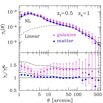
where we have taken the flat-sky limit, which is very accurate for practically all angular scales (i.e., few degrees). The exact expression can be obtained by simply replacing the Bessel functions above by Legendre polynomials (see de Putter & Takada (2010)). In Fig.10 we show results for the tangential shear measured in the dark-matter and the mock galaxies, for a source galaxy sample at and a lens population at . Non-linear effects, that become important at armcin, are well captured in the simulations. In the lower panel of Fig.10 we see that MICE-GC dark-matter has more power than predicted by Halofit on non-linear scales, but it shows a lack of power relative to the revised Halofit prediction, what is consistent with our findings for the convergence power spectrum, Fig.2. We also show the result of scaling up both the Halofit (dotted) and revised Halofit (dot-dashed) predictions, with the linear galaxy bias, , estimated form the lens galaxy population (see Fig.9). Our measurement of the galaxy tangential shear is in rough agreement with the linearly biased Halofit prediction, although they disagree on the smallest scales, where the simple linear bias assumption seems to break down.
On the other hand, a common observable in lensing surveys is the 2-point shear correlation functions, , which in turn are related to the tangential and cross-component of the shear,
| (13) |
where, , and , and is the polar angle of the separation vector, .
In the weak lensing limit (i.e., in the absence of rotational modes) these shear correlations are related to the the gradient or E-mode component of the shear tensor (see Bartelmann & Schneider (2001)),
| (14) |
where we have assumed the Limber approximation, for which its also true that the shear and convergence power spectra are identical, , as explicitly shown in Fig.4. We can thus compute by using the convergence power spectra. Note that this in turn is saying that both shear correlation functions are not independent, as they are both related to the same underlying lensing potential. In fact, one can easily invert Eq.(14) to get (e.g., Schneider (2003)),
| (15) | |||||
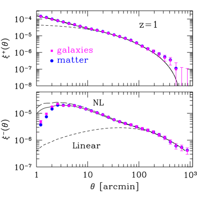
Figure 11 shows the shear 2-point correlation functions for sources at . For we see that both MICE-GC mock galaxies and dark-matter are in close agreement with the non-linear prediction, as they deviate from the purely linear regime for arcmin, and down to arcmin scales. In particular, predictions from Halofit (solid line) and the revised Halofit (long-dashed) can be hardly distinguished on these non-linear scales. The agreement between the simulation and theory is even more remarkable for , for which non-linear effects become significant at much larger scales, arcmin, in much the same way it happened for the tangential shear, Fig.10.
5 Magnification from Galaxy cross-correlations
Gravitational lensing by large-scale structures in the universe changes the number density of background sources and thus it induces a cross-correlation signal between background and foreground galaxy populations (Moessner & Jain, 1998; Bartelmann & Schneider, 2001). Such cross-correlations have been measured using samples of distant quasars magnified by low redshift galaxies (e.g., Benitez & Martinez-Gonzalez (1997); Gaztañaga (2003); Myers et al. (2005); Scranton et al. (2005)), that can be used to put constraints on the galaxy-mass power spectrum (Jain et al., 2003).
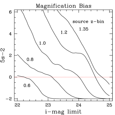
For a magnitude limited survey, the cumulative number of galaxies above a flux limit scales as , where is the area of the survey, and is the power-law slope of the background number counts. Lensing preserves the surface brightness of galaxies by increasing the observed survey depth (i.e, decreasing the effective flux limit) and the effective survey area by the same amount: , , where is the magnification. These two competing effects induce the so-called magnification bias in the cumulative number of background sources,
| (16) |
In the weak-lensing limit, where , and we can Taylor expand, and therefore the magnified overdensity of background sources is given by,
| (17) | |||||
where in the last equality, we have used the simple relation between the fluctuations in magnification and convergence of dark-matter counts, , that is valid in the weak-lensing limit. Note that in we have defined the two qualitatively different contributions:
-
1.
counts from magnified magnitudes,
(18) -
2.
counts from lensed positions
(19)
These two contributions cannot be separated observationally, but we define two different galaxy samples accordingly in our simulation in order to validate the two magnification contributions separately. Above, we have defined the the logarithmic slope of the background number counts at redshift , for a magnitude limit ,
| (20) |
The net magnification from these two competing effects depends on how the loss of sources due to the area dilution, , is compensated by the gain of sources from the flux magnification, . Number counts for source populations with flat luminosity functions, such as faint galaxies, decrease due to magnification, whereas sources with steep luminosity functions, such as quasars, increase. Note that, in the particular case when , then , and there is no net magnification effect.
5.1 Implementation in galaxy mocks
Below we describe how to implement magnification in the magnitudes and positions of mock galaxies.
-
1.
magnified magnitudes: flux magnification makes the mock galaxy magnitudes, , brighter by an amount,
(21) where in the last equality we have Taylor expanded and used the fact that in the weak-lensing limit. Therefore, knowing the value of the convergence, , at a given point in the source plane, it is straightforward to compute the flux magnification induced, that in turn produces the change in the background number counts, .
-
2.
magnified or lensed positions: the “observed” or lensed position, , of a light ray is shifted from the “true” or unlensed position, , by an angle given by the deflection vector, , according to the lens equation on the source plane (see e.g., Bartelmann & Schneider (2001)). In the single-plane (or Born) approximation, the lens equation reads,
(22) where the deflection vector, is a tangent vector at the unlensed position of the light ray, and the lensed position is found by moving along a geodesic on the sphere in the direction of this tangent vector and for an arc length given by the deflection angle, . If we denote the unlensed position on the sphere by , then the lensed position, , can be simply derived by using identities of spherical triangles (Lewis, 2005; Das & Bode, 2008),
(23) where the (complex) deflection vector is projected on the polar basis of the sphere, , at the unlensed position as,
(24) being the angle between the deflection vector and the polar basis vector . We use Eq.(23) above to re-map source galaxy positions due to the lensing by the large-scale structure in the lightcone Nbody simulation.
5.2 Validation
We consider two different observable sources for magnification: counts and magnitudes. In both cases we correlate foreground density (counts) fluctuations. In the former we also use counts for the background while in the later we use fluctuations in the background magnitudes.
5.2.1 Counts
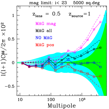
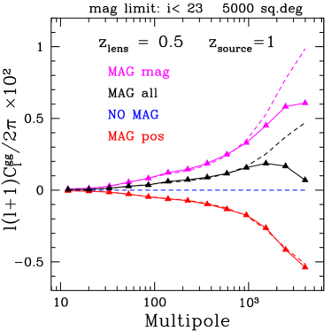
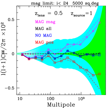
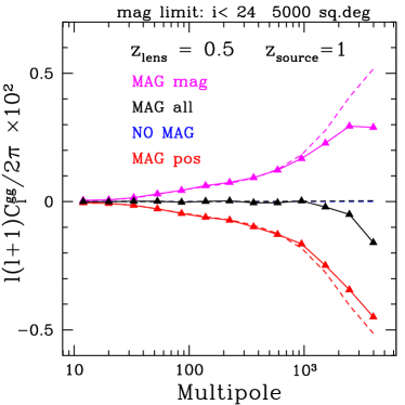
In order to validate the magnification signal in the simulation, we have selected a magnitude limited sample from the parent HOD mock, by imposing a cut in the band (which is in principle less affected by non-cosmological signals such as dust extinction), and have constructed four different cross-correlation pairs between foreground counts (lenses) and background counts (source) galaxies, well separated in redshift:
where and are given by Eqs.(18)-(19) respectively. For both the predictions and simulations we take: , so that lenses are at a sufficiently low redshift that they are negligibly magnified. In fact, lens magnification contributes to the cross-correlation signal at the percent level only for at (Ziour & Hui, 2008). Therefore the cross-correlation between (magnified) source and (un-magnified) lens galaxy populations are given by (see Eq.(17) ,
| (25) | |||||
We can thus predict the magnification signal expected by using the non-linear matter cross-correlations, (we use Halofit as implemented in CAMB sources), scaled by the factor, , where is the linear bias derived from the auto-correlation of the lens galaxy population (see Fig. 9), and the magnification bias of the source galaxy sample (see Fig. 12).
Figure 13 shows the measurements in MICE-GC for these four pairs separately, for lenses located at , ie., the peak of the weak-lensing efficiency for sources at . We choose bin widths , centered at and , to include enough galaxies in each source/lens bin to minimize the impact of shot-noise in the cross-correlation errors. We display two illustrative cases: top panels of Fig.13 show the case for for which theory predicts a magnification bias (see Fig.12), and thus a large positive cross-correlation induced by magnification. This is further enhanced by the galaxy bias factor of the lenses, as the galaxy cross-correlations are given by on Lower panels show a null magnification test, i.e., the case when the magnification bias vanishes. Overall we find good agreement between theoretical predictions (dashed lines) and simulations (open symbols) in both test cases. Magnification from a single cross-correlation pair is noise dominated for all the dynamical range: 1- statistical Gaussian errors are shown by shaded areas. Shot-noise (inner green shaded) dominates on small-scales (i.e., high multipoles) whereas sample variance dominates the total error (cyan shaded) on large scales (i.e., low multipoles).
In order to suppress the sample variance contribution that dominates the cross-correlations on basically all-scales, we shall take the difference in cross-correlation pairs that see approximately the same sky realization. For example, to estimate the magnified positions (MAG mag) pair above without sample-variance, we equate,
| (26) |
This is shown to bring simulation measurements in much better agreement with theory predictions for all the dynamical range. The cosmic-variance-free measurement, Eq. (26), is shown in the right panels of Figure 13, as compared direct cross-correlation pair (top panel), down to the scales that are affected by the pixel scale of the maps, . Other cosmic-variance-free pairs are also shown in the same figure (see filled symbols). Note however that this trick only works approximately: one small-enough scales (i.e., few arcmins), the lensed sky is different than the unlensed one (i.e., due precisely to the lensing of background sources) and thus the sample variance affecting lensed and unlensed galaxy populations is slightly different. This could explain why on few arcmin scales, the cosmic-variance free measurement to be in disagreement with theory expectations for each of the samples cross-correlated. A more detailed analysis of simulated magnification measurements from cross-correlations of galaxies will be presented elsewhere.
5.2.2 Magnitudes
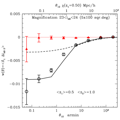
In Fig.14 we show the cross-correlation of foreground densities with background magnitudes: . This signal is expected to be proportional to for the same sample, shown in Fig.8:
| (27) |
where the proportionality constant is:
| (28) |
where is the mean magnitude in the (source) redshift bin under consideration and is the magnitude limit in our selection. In Fig.14 we apply magnification to positions and also to magnitudes, but we select galaxies according to the true magnitudes, in the range and . That way and we can measure directly the effect of magnification on individual magnitudes. If we use magnified (ie observed) magnitudes to select the MICE galaxies we find , close to the values found in Ménard et al. (2010) for QSO or Bauer et al. (2013) for LRG galaxies. In such case we find that the measurement scales with , as expected.
Fig.14 shows a good agreement with the non-linear DM prediction, shown as a continuous line. The dashed line is for linear theory. These predictions are the same as the lines in Fig.8, scaled by . The closed triangles show the measurement without magnification in the magnitudes, which yields zero correlation, as expected. Positions are also altered by magnification for both triangles and circles, but this produces no signal when we use magnitudes instead of counts. Note that the error-bars (for a 5x100 sq.deg. survey) are much smaller here than in the case of the counts in Fig. 13. This is because the intrinsic correlation of magnitudes in the sources are more weakly correlated than the counts and this reduces the sampling variance in the cross-correlation error.
6 Conclusions
In paper I of this series (Fosalba et al. (2015)) we presented the MICE Grand Challenge Lightcone simulation (MICE-GC), one of the largest Nbody runs completed to date. It contains about 70 billion particles in a 3 periodic box. This unique combination of large volume and fine mass resolution allows to resolve the growth of structure form the largest (linear) cosmological scales down to very small ( tens of Kpcs) scales, well within the non-linear regime. Therefore, the MICE-GC presents multiple potential applications to study the clustering and lensing properties of dark-matter and galaxies over a wide dynamical range, that can be confronted with observations from wide and deep galaxy surveys.
Paper II (Crocce et al. (2015)) presented and validated the FoF halo catalogs obtained from the MICE-GC. These halo catalogs were populated with galaxies using a HOD+SAM technique over one octant of the sky (i.e., 5000 sq.deg) and to the full depth of the lightcone, . Extensive properties where also attributed to this galaxy mock, named MICECAT v1.0, whose clustering was later throughly validated using 2 and 3-point statistics.
In the last paper of this series (Paper III) we have described the construction of high spatial (sub-arcmin) resolution all-sky lensing maps from the MICE-GC lightcone simulation outputs, and discuss their application to model galaxy lensing properties of the MICECAT mock catalog. These properties, including the convergence, shear, and lensed magnitudes and positions, have been validated using various lensing observables in harmonic and real space. In particular, we have studied auto and cross correlations of both dark-matter and galaxy samples.
Below we provide the main findings from this extensive analysis of the all-sky lensing maps and derived galaxy lensing mocks:
-
•
Mass resolution effects observed in the angular clustering of projected dark-matter in the lightcone (see Paper I, Fosalba et al. (2015)), are expected to build up in lensing observables, as they integrate contributions of all matter shells along the line of sight. This qualitative picture is confirmed using the lensing maps produced from the MICE simulations (see Fig5): the smallest mass halos resolved in the higher resolution run, , which have diameter of 2 Mpc/h, are not found in previous (lower-mass resolution) runs. As a consequence, and in the language of the halo model, the 1-halo contribution to the angular power spectra of the convergence (or shear) field is substantially suppressed for the low-resolution realizations at the angular scales subtended by these halos, typically few arcminutes in the sky. This is shown in Fig.2 where comparison of the measured power in MICE-GC with respect to the lower-resolution MICE-IR run implies that mass-resolution effects are at the 5 level for and 20 for .
-
•
We find an excess of convergence power for sources at in the MICE-GC relative to Halofit (Smith et al., 2003), at the level for , as shown in Fig.2. This is consistent with a similar analysis from the higher-resolution Millennium Simulation (Hilbert et al., 2009). On the other hand, other recent high-resolution simulations seem to find an even larger power excess at this highly non-linear scales (see Takahashi et al. (2012)).
-
•
We have also modelled the lensing properties of synthetic galaxies using the MICE-GC lightcone simulation up to , using the “onion universe” approach (see Fosalba et al. (2008)) that is equivalent to ray-tracing techniques in the Born approximation. We have tested the accuracy of our simulation by comparing the auto-correlation of the convergence and the galaxy counts-convergence cross-correlation to current numerical fits. Fig.7 and 14 show that for a magnitude limited source sample at there is very good match between MICE and Halo-model fits from linear scales down to the resolution or pixel scale (i.e, about 1 arcmin.) of the angular maps used for the analysis. In particular, a simple linear galaxy bias of matches the measured cross-correlation, in agreement with the bias factor estimated from the foreground galaxy sample auto-correlation at (see Fig.9)
-
•
Comparison of the 2-point shear correlation functions measured in MICE to halo-model fits shows that our simulation is accurate down to arcmin scales. The MICE-GC measurements underestimate recent theory fits based on high-resolution simulations (Takahashi et al., 2012) by on arcmin scales, and overpredicts lower resolution halo-model fits (Smith et al., 2003) by a similar amount.
-
•
In this paper we have also introduced for the first time the modeling of the magnification effect on the observed positions of background galaxies using all-sky lensing maps. This “area dilution” effect induces a measurable anti-correlation between foreground and distant background galaxy samples. The magnification effect in galaxy positions has opposite sign with respect to the flux magnification by foreground sources in magnitude limited samples, and therefore the net lensing effect on distant galaxies, known as magnification bias depends on the slope of the background population source counts, as shown in Fig.12.
-
•
By taking different magnitude limited galaxy samples we have compared the two qualitatively different contributions to the magnification bias in MICE as compared to theoretical predictions (in the Born approximation). As shown in left panels of Fig.13, simulation results match well the theory in all the dynamical range (i.e, almost three decades in angular scale). The oscillations observed in simulation measurements are believed to be due to the large sample variance that affects the cross-correlations (ie., auto-correlations contributing to the noise are comparable to the signal). This is confirmed in the right panels which show that when building “sample variance free” combinations of correlations, the match between simulations and theory is significantly improved (see text for details).
-
•
We also present for the first time the modeling of cross-correlations between foreground counts with (magnified) background magnitudes. Our anlaysis shows good agreement between simulation measurements and theory expectations, as depicted in Fig.14. The error-bars are much smaller here than in the case of magnification bias above. This is because the intrinsic correlation of magnitudes in the sources are more weakly correlated than the counts and this reduces the sampling variance in the cross-correlation error. This and the points above show that our modeling of magnification in galaxy positions can be safely used down to arcminute scales.
We are making a first public data release of the MICE-GC Galaxy mocks, MICECAT v1.0, including the lensing properties described in this paper, through a dedicated webportal, http://cosmohub.pic.es. This new galaxy mock should serve as a powerful tool to model the clustering and lensing observables expected from upcoming large astronomical surveys in the era of precision cosmology.
Acknowledgments
We would like to thank Christopher Bonnett, Antony Lewis, Guilhem Lavaux and Carlos Lopez for useful discussions. We are greatly indebted to Jorge Carretero, Christian Neissner, Davide Piscia, Santi Serrano and Pau Tellada for their development of the CosmoHub web-portal. We acknowledge support from the MareNostrum supercomputer (BSC-CNS, www.bsc.es), through grants AECT-2008-1-0009, 2008-2-0011, 2008-3-0010, 2009-1-0009, 2009-2-0013, 2009-3-0013, and Port d’Informació Científica (PIC, www.pic.es) where the simulations were ran and stored, respectively. The MICE simulations were implemented using the Gadget-2 code (www.mpa-garching.mpg.de/gadget). Funding for this project was partially provided by the European Commission Marie Curie Initial Training Network CosmoComp (PITN-GA-2009 238356), the Spanish Ministerio de Ciencia e Innovacion (MICINN), projects 200850I176, AYA-2009-13936, AYA-2012-39620, AYA-2012-39559, Consolider-Ingenio CSD2007-00060 and research project SGR-1398 from Generalitat de Catalunya. MC acknowledges support from the Ramón y Cajal MICINN program.
References
- Albrecht (2006) Albrecht A., 2006, in APS April Meeting Abstracts Report from the Dark Energy Task Force. p. G1002
- Albrecht & Bernstein (2007) Albrecht A., Bernstein G., 2007, Phys. Rev. D , 75, 103003
- Bartelmann (2010) Bartelmann M., 2010, Classical and Quantum Gravity, 27, 233001
- Bartelmann & Schneider (2001) Bartelmann M., Schneider P., 2001, Phys. Rep. , 340, 291
- Bauer et al. (2013) Bauer H., Gaztanaga E., Marti P., Miquel R., 2013, ArXiv 1312.2458
- Becker (2013) Becker M. R., 2013, MNRAS , 435, 115
- Benitez & Martinez-Gonzalez (1997) Benitez N., Martinez-Gonzalez E., 1997, Astrophys. J. , 477, 27
- Blandford et al. (1991) Blandford R. D., Saust A. B., Brainerd T. G., Villumsen J. V., 1991, MNRAS , 251, 600
- Cabré et al. (2007) Cabré A., Fosalba P., Gaztañaga E., Manera M., 2007, MNRAS , 381, 1347
- Cooray & Hu (2001) Cooray A., Hu W., 2001, Astrophys. J. , 554, 56
- Crocce et al. (2011) Crocce M., Cabré A., Gaztañaga E., 2011, MNRAS , 414, 329
- Crocce et al. (2015) Crocce M., Castander F. J., Gaztanaga E., Fosalba P., Carretero J., 2015, ArXiv 1312.2013
- Crocce et al. (2010) Crocce M., Fosalba P., Castander F. J., Gaztañaga E., 2010, MNRAS , 403, 1353
- Das & Bode (2008) Das S., Bode P., 2008, Astrophys. J. , 682, 1
- de Putter & Takada (2010) de Putter R., Takada M., 2010, Phys. Rev. D , 82, 103522
- Fosalba et al. (2015) Fosalba P., Crocce M., Gaztañaga E., Castander F. J., 2015, MNRAS , 448, 2987
- Fosalba et al. (2008) Fosalba P., Gaztañaga E., Castander F. J., Manera M., 2008, MNRAS , 391, 435
- Gaztañaga (2003) Gaztañaga E., 2003, Astrophys. J. , 589, 82
- Gaztanaga & Bernardeau (1998) Gaztanaga E., Bernardeau F., 1998, A&A , 331, 829
- Górski et al. (2005) Górski K. M., Hivon E., Banday A. J., Wandelt B. D., Hansen F. K., Reinecke M., Bartelmann M., 2005, Astrophys. J. , 622, 759
- Hamana et al. (2002) Hamana T., Colombi S. T., Thion A., Devriendt J. E. G. T., Mellier Y., Bernardeau F., 2002, MNRAS , 330, 365
- Harnois-Déraps et al. (2012) Harnois-Déraps J., Vafaei S., Van Waerbeke L., 2012, MNRAS , 426, 1262
- Hilbert et al. (2009) Hilbert S., Hartlap J., White S. D. M., Schneider P., 2009, A&A , 499, 31
- Hoekstra & Jain (2008) Hoekstra H., Jain B., 2008, Annual Review of Nuclear and Particle Science, 58, 99
- Hu (2000) Hu W., 2000, Phys. Rev. D , 62, 043007
- Jain et al. (2003) Jain B., Scranton R., Sheth R. K., 2003, MNRAS , 345, 62
- Jain et al. (2000) Jain B., Seljak U., White S., 2000, Astrophys. J. , 530, 547
- Jeong et al. (2009) Jeong D., Komatsu E., Jain B., 2009, Phys. Rev. D , 80, 123527
- Kaiser (1992) Kaiser N., 1992, Astrophys. J. , 388, 272
- Kilbinger (2013) Kilbinger e. a., 2013, MNRAS , 430, 2200
- Lavaux & Wandelt (2010) Lavaux G., Wandelt B. D., 2010, Astrophys. J. Suppl. , 191, 32
- Lewis (2005) Lewis A., 2005, Phys. Rev. D , 71, 083008
- Ménard et al. (2010) Ménard B., Scranton R., Fukugita M., Richards G., 2010, MNRAS , 405, 1025
- Moessner & Jain (1998) Moessner R., Jain B., 1998, MNRAS , 294, L18
- Myers et al. (2005) Myers A. D., Outram P. J., Shanks T., Boyle B. J., Croom S. M., Loaring N. S., Miller L., Smith R. J., 2005, MNRAS , 359, 741
- Sato et al. (2009) Sato M., Hamana T., Takahashi R., Takada M., Yoshida N., Matsubara T., Sugiyama N., 2009, Astrophys. J. , 701, 945
- Schneider (2003) Schneider P., 2003, ArXiv Astrophysics e-prints
- Scoccimarro et al. (1999) Scoccimarro R., Zaldarriaga M., Hui L., 1999, Astrophys. J. , 527, 1
- Scranton et al. (2005) Scranton R., Ménard B., Richards G. T., Nichol R. C., Myers A. D., Jain B., Gray A., Bartelmann M., Brunner R. J., Connolly A. J., Gunn J. E., Sheth R. K., Bahcall N. A., Brinkman J., Loveday J., Schneider D. P., Thakar A., York D. G., 2005, Astrophys. J. , 633, 589
- Semboloni et al. (2007) Semboloni E., van Waerbeke L., Heymans C., Hamana T., Colombi S., White M., Mellier Y., 2007, MNRAS , 375, L6
- Smith et al. (2003) Smith R. E., Peacock J. A., Jenkins A., White S. D. M., Frenk C. S., Pearce F. R., Thomas P. A., Efstathiou G., Couchman H. M. P., 2003, MNRAS , 341, 1311
- Springel (2005) Springel V., 2005, MNRAS , 364, 1105
- Stebbins (1996) Stebbins A., 1996, ArXiv astro-ph/9609149
- Takada & Jain (2009) Takada M., Jain B., 2009, MNRAS , 395, 2065
- Takahashi et al. (2012) Takahashi R., Sato M., Nishimichi T., Taruya A., Oguri M., 2012, Astrophys. J. , 761, 152
- Teyssier et al. (2009) Teyssier R., Pires S., Prunet S., Aubert D., Pichon C., Amara A., Benabed K., Colombi S., Refregier A., Starck J.-L., 2009, A&A , 497, 335
- Vale & White (2003) Vale C., White M., 2003, Astrophys. J. , 592, 699
- Van Waerbeke et al. (2001) Van Waerbeke L., Hamana T., Scoccimarro R., Colombi S., Bernardeau F., 2001, MNRAS , 322, 918
- Van Waerbeke & Mellier (2003) Van Waerbeke L., Mellier Y., 2003, ArXiv astro-ph/0305089
- Wambsganss et al. (1998) Wambsganss J., Cen R., Ostriker J. P., 1998, Astrophys. J. , 494, 29
- Weinberg et al. (2013) Weinberg D. H., Mortonson M. J., Eisenstein D. J., Hirata C., Riess A. G., Rozo E., 2013, Phys. Rep. , 530, 87
- White & Hu (2000) White M., Hu W., 2000, Astrophys. J. , 537, 1
- White & Vale (2004) White M., Vale C., 2004, Astroparticle Physics, 22, 19
- Ziour & Hui (2008) Ziour R., Hui L., 2008, Phys. Rev. D , 78, 123517