Spectral Renormalization Group for the Gaussian model and ψ4superscript𝜓4\psi^{4} theory on non-spatial networks

Aslı Tuncer1,2 and Ayşe Erzan1 1Department of Physics, Istanbul Technical University, Maslak 34469, Istanbul, Turkey
2Department of Physics, Işık University, Şile 34980, Istanbul, Turkey
Abstract

We implement the spectral renormalization group on different deterministic non-spatial networks without translational invariance. We calculate the thermodynamic critical exponents for the Gaussian model on the Cayley tree and the diamond lattice, and find that they are functions of the spectral dimension, d~~𝑑\tilde{d}. The results are shown to be consistent with those from exact summation and finite size scaling approaches. At d~=2~𝑑2\tilde{d}=2, the lower critical dimension for the Ising universality class, the Gaussian fixed point is stable with respect to a ψ4superscript𝜓4\psi^{4} perturbation up to second order. However, on generalized diamond lattices, non-Gaussian fixed points arise for 2<d~<42~𝑑42<\tilde{d}<4.

PACS Nos: 2.10.Ox,89.75.Da,89.75.Hc

I Introduction

Both static and dynamical phenomena on networks, which typically lack translational invariance and may not be naturally embedded in a metric space, have been the subject of intense study over the last decade and a half  BA_book ; Vespignani_largescale ; Vespignani_Dynamical . Phase transitions and critical phenomena on networks have also received a lot of attention  BA ; dorogovtsev1 .

To date, a unified approach to the theory of critical phenomena on arbitrary networks, analogous to the renormalization group theory developed by Wilson and Kogut Wilson1 ; Wilson2 ; Wilson_F ; Wilson3 on periodic networks, is still lacking. The outstanding achievement of the renormalization group (RG) theory of critical phenomena was to explain the experimentally observed phenomenon of “universality” and introduce such concepts as the “relevance” or “irrelevance” of different types of interactions, upper and lower critical dimensions and the elucidation of the roles of the dimensionality of space and of the order parameter.

Dorogovsev et al. dorogovtsev1 have shown how the critical behavior of scale free graphs depends on the scaling exponent γ𝛾\gamma of the degree distribution, and Bradde et al. Bianconi2010 have derived a Ginzburg criterion in terms of an effective spectral dimension for spatial scale free networks. Various “real space renormalization group” (RSRG) Leeuwen ; Burkhardt ; newKadanoff methods have been proposed for arbitrary networks Havlin , but even when they are exact, they rarely reveal universal properties of critical phenomena on non-spatial networks in terms of their spectral and topological properties, and there is still room for improving our understanding.

In a recent publication erzan we have proposed a spectral renormalization group (SRG) scheme modelled on the “momentum shell” renormalization group a là Wilson Wilson3 . We expand the fluctuations of the order parameter in terms of the eigenvectors of the graph Laplacian Chung in a generalized Fourier transform, partly surmounting the difficulty posed by non-translationally invariant lattices. Elimination of the large eigenvalue fluctuations and rescaling of the effective Hamiltonian then yield, in the same spirit as in the Wilson renormalization group, the rescaling factors for the coupling constants, which can then be related to the critical exponents.

On non-translationally invariant, non-spatial networks, the eigenvalues of the graph Laplacian do not have an obvious interpretation in terms of lattice momenta and an isotropic, translationally invariant correlation length is not available. Therefore the exponent of the RG eigenvalue in the temperature-like direction under length- rescaling cannot be naively interpreted in terms of an inverse correlation length exponent. We have to develop RG schemes which do not involve length-like concepts.

In this paper, we explicitly implement the SRG erzan on two non-spatial networks which lack translational invariance, namely, the Cayley tree and the diamond lattice diamond for Gaussian model Berlin ; Huang ; Goldenfeld . Then we include a quartic interaction term, which on periodic lattices is known to carry the “trivial” theory into the Ising universality class.Wilson3 ; Amit and we investigate the renormalization behavior of the interacting theory within a perturbation expansion up to the second order in the coupling constant and the deviation from the critical temperature.

We find that for the Gaussian theory, the critical exponents depend only on the spectral dimension of the lattice, i.e., the scaling behavior of the small eigenvalue region of the Laplace spectrum. However, the interacting theory depends sensitively on the symmetry properties of the lattice, via the eigenvectors of the graph Laplacian, which enter the calculations of the four-vertex.

Within second order perturbation theory we find that the Gaussian fixed point is stable at d~~𝑑\tilde{d}. Extending our calculations to a series of generalized diamond lattices with higher spectral dimensions, we establish the existence of non-trivial fixed point of the SRG for 2<d~< 42~𝑑42\,<\,\tilde{d}\,<\,4.

In Section II, we define the spectral renormalization group for the Gaussian model on a generic network. In Section III, we implement this scenario on the Cayley tree and the diamond (hierarchical) lattice. We compute the specific heat and magnetic field exponents. For comparison, exact enumeration and finite size scaling results are presented in Section IV. In Section V we include ψ4superscript𝜓4\psi^{4} interactions. In Section VI we provide a discussion and conclusions.

II The Spectral Renormalization Group for the Gaussian Model

The effective Ginzburg-Landau “Lagrangian” for a scalar order parameter ψ(𝐱)𝜓𝐱\psi(\mathbf{x}) is given by,

H=Vd𝐱{12[r0ψ2(𝐱)ψ(𝐱)2ψ(𝐱)]+v0ψ4(𝐱)hψ(𝐱)}.𝐻subscript𝑉𝑑𝐱12delimited-[]subscript𝑟0superscript𝜓2𝐱𝜓𝐱superscript2𝜓𝐱subscript𝑣0superscript𝜓4𝐱𝜓𝐱\begin{split}H=\int_{V}d{\mathbf{x}}\{\frac{1}{2}\left[r_{0}\psi^{2}(\mathbf{x})-\psi(\mathbf{x})\nabla^{2}\psi(\mathbf{x})\right]+\\ v_{0}\psi^{4}(\mathbf{x})-h\psi(\mathbf{x})\}\;\;.\end{split} (1)

where the integral is over the volume of the system, r0subscript𝑟0r_{0} is proportional to the reduced temperature t=(TTc)/Tc𝑡𝑇subscript𝑇𝑐subscript𝑇𝑐t=(T-T_{c})/T_{c} and hh to the magnetic field. We will assume that H𝐻H is expressed in units of the thermal energy kBTsubscript𝑘𝐵𝑇k_{B}T where kBsubscript𝑘𝐵k_{B} is the Boltzmann constant. The Gaussian model Berlin is equivalent to omitting the fourth order coupling term in Eq. (1). This model is defined only for temperatures above the critical temperature, i.e., for r0>0subscript𝑟00r_{0}>0. Nevertheless one may formally compute the exponent δ𝛿\delta.

For a continuous field ψ(i)(,)𝜓𝑖\psi(i)\in(-\infty,\infty), living on the nodes of an arbitrary network, the Gaussian model can be written as

H0=12ijNψ(i)[r0δij+Lij]ψ(j)hiψ(i).subscript𝐻012superscriptsubscript𝑖𝑗𝑁𝜓𝑖delimited-[]subscript𝑟0subscript𝛿𝑖𝑗subscript𝐿𝑖𝑗𝜓𝑗subscript𝑖𝜓𝑖H_{0}=\frac{1}{2}\sum_{ij}^{N}\psi(i)[r_{0}\delta_{ij}+L_{ij}]\psi(j)-h\sum_{i}\psi(i)\;\;. (2)

The usual Laplace operator appearing in the Ginzburg-Landau expansion has been replaced by (minus) the graph Laplacian Chung , with the matrix elements,

Lij=diδijAij,subscript𝐿𝑖𝑗subscript𝑑𝑖subscript𝛿𝑖𝑗subscript𝐴𝑖𝑗L_{ij}=d_{i}\delta_{ij}-A_{ij}\;\;, (3)

where 𝐀𝐀{\bf A} is the adjacency matrix of the network and disubscript𝑑𝑖d_{i} is the degree of the i𝑖ith node. The expression in Eq. (2) is now very general, applicable to arbitrary networks, with only the requirement that the matrix 𝐀𝐀{\bf A} be symmetric, so that its eigenvalues are real.

Expanding the field ψ(i)𝜓𝑖\psi(i) in terms of eigenvectors 𝐮μsubscript𝐮𝜇\mathbf{u}_{\mu} of the Laplace operator, ψ(i)=N1/2μψ^μuμ(i)𝜓𝑖superscript𝑁12subscript𝜇subscript^𝜓𝜇subscript𝑢𝜇𝑖\psi(i)=N^{-1/2}\sum_{\mu}\hat{\psi}_{\mu}u_{\mu}(i), the Hamiltonian is obtained in diagonal form,

H0=12μ=1N[r0+ωμ]ψ^μ2hψ^1.subscript𝐻012superscriptsubscript𝜇1𝑁delimited-[]subscript𝑟0subscript𝜔𝜇superscriptsubscript^𝜓𝜇2subscript^𝜓1H_{0}=\frac{1}{2}\sum_{\mu=1}^{N}[r_{0}+\omega_{\mu}]\hat{\psi}_{\mu}^{2}-h\hat{\psi}_{1}\;\;. (4)

Here ωμsubscript𝜔𝜇\omega_{\mu} are the eigenvalues of 𝐋𝐋{\bf L}. The eigenvalues are ordered so that ω1ω2ωNsubscript𝜔1subscript𝜔2subscript𝜔𝑁\omega_{1}\leq\omega_{2}\ldots\leq\omega_{N}, with ω1=0subscript𝜔10\omega_{1}=0. We will assume the network to be connected so that ω2>0subscript𝜔20\omega_{2}>0 for finite N𝑁N.

For this system, the partition function is immediately obtained from

Z0=μdψ^μeH0,subscript𝑍0superscriptsubscriptsubscriptproduct𝜇𝑑subscript^𝜓𝜇superscript𝑒subscript𝐻0Z_{0}=\int_{-\infty}^{\infty}\prod_{\mu}d\hat{\psi}_{\mu}e^{-H_{0}}\;\;, (5)

and the free energy is given, up to constant terms, by

F0=12μ=1Nln(r0+ωμ)h22r0.subscript𝐹012superscriptsubscript𝜇1𝑁subscript𝑟0subscript𝜔𝜇superscript22subscript𝑟0F_{0}=\frac{1}{2}\sum_{\mu=1}^{N}\ln(r_{0}+\omega_{\mu})-\frac{h^{2}}{2r_{0}}\;\;. (6)

(Henceforth we will drop the external field term unless we are directly dealing with it.)

Note that in Eq.(4) there is a difficulty in going over from a sum (over μ=1,,N𝜇1𝑁\mu=1,\ldots,N) to an integral over the eigenvalues. In general the eigenvectors 𝐮μsubscript𝐮𝜇\mathbf{u}_{\mu}, and consequently the ψ^μsubscript^𝜓𝜇\hat{\psi}_{\mu}, do not possess, e.g., the rotational symmetries valid on periodic lattices. Therefore in general it is not justified to try to extract the renormalization factors by rewriting the Hamiltonian as,

120Ω𝑑ωρ(ω)[r0+ω]ψ^ω2,12superscriptsubscript0Ωdifferential-d𝜔𝜌𝜔delimited-[]subscript𝑟0𝜔superscriptsubscript^𝜓𝜔2\frac{1}{2}\int_{0}^{\Omega}d\omega\rho(\omega){[r_{0}+\omega]\hat{\psi}_{\omega}^{2}}\;\;, (7)

where ΩΩ\Omega is the largest eigenvalue. On the other hand, after the Gaussian integrals have been carried out, this difficulty is not there for the free energy (or its derivatives, such as the specific heat or the two-point correlation function Hattori ) and one may formally write,

F0=120Ω𝑑ωρ(ω)ln(r0+ω).subscript𝐹012superscriptsubscript0Ωdifferential-d𝜔𝜌𝜔subscript𝑟0𝜔F_{0}=\frac{1}{2}\int_{0}^{\Omega}d\omega\rho(\omega)\ln(r_{0}+\omega)\;\;. (8)

We would now like to show how we can implement field theoretic renormalization group ideas on a system which, besides not having an a priori known spectral density, is not embedded in a metric space, i.e., there is no concept of length.

We have two possible strategies for eliminating the large ω𝜔\omega fluctuations from the partition function and computing the renormalization factors. In the absence of a “length like” quantity, the first method which comes to mind is to truncate the number of modes, N𝑁N, by a constant factor, successively integrating out those with the the largest eigenvalues. The second method consists of scaling the largest eigenvalue, ΩΩ\Omega by a constant B𝐵B, in analogy with the usual renormalization group a là Wilson Wilson1 ; Wilson2 ; Wilson3 ; Goldenfeld . These two strategies are implemented below, and give identical results for the Gaussian model.

It should be noted that on these non-spatial lattices, eigenvectors with the same symmetry properties may have widely differing eigenvalues. (We illustrate this in Table A.1 in the Appendix, for N=13𝑁13N=13 on the Cayley tree. A similar situation also holds for the diamond lattice.) Eliminating those fluctuations associated with the high-ω𝜔\omega side of the spectrum makes sense in terms of eliminating the higher-energy modes but cannot be naively interpreted as eliminating the “small wavelength” or “high frequency” fluctuations. On the other hand, if we interpret the successive iterations in the construction of trees or hierarchical lattices as a fine-graining operation GriffithsandKaufman , the increasing localization of the eigenvectors on the most recently added nodes may be thought of as greater articulation on smaller scales.

II.1 Scaling the number of modes

Since the eigenvalues are numbered in increasing order by convention, we keep the first N/B𝑁𝐵N/B eigenvalues in the effective Hamiltonian and integrate out the rest. Picking the scale factor B𝐵B in keeping with the overall symmetries of the system is convenient; if no such obvious scale symmetry is available, B=N/n𝐵𝑁𝑛B=N/n, with n𝑛n integer, eliminates spurious points from the scaling plots. Defining the cutoff μB=N/Bsubscript𝜇𝐵𝑁𝐵\mu_{B}=N/B, the truncated Hamiltonian is,

H0<=12μ=1μB[r0+ωμ]ψ^μ2hψ^1.superscriptsubscript𝐻012superscriptsubscript𝜇1subscript𝜇𝐵delimited-[]subscript𝑟0subscript𝜔𝜇superscriptsubscript^𝜓𝜇2subscript^𝜓1H_{0}^{<}=\frac{1}{2}\sum_{\mu=1}^{\mu_{B}}[r_{0}+\omega_{\mu}]\hat{\psi}_{\mu}^{2}-h\hat{\psi}_{1}\;\;. (9)

Restoring the Hamiltonian to its full range calls for rescaling factors to be inserted, viz.,

H0=12μ=1N[r0Bϕ1+Bϕ1ϕ2ωμ](ψ^μ)2hψ^1.superscriptsubscript𝐻012superscriptsubscript𝜇1𝑁delimited-[]subscript𝑟0superscript𝐵subscriptitalic-ϕ1superscript𝐵subscriptitalic-ϕ1subscriptitalic-ϕ2subscript𝜔𝜇superscriptsuperscriptsubscript^𝜓𝜇2superscriptsuperscriptsubscript^𝜓1H_{0}^{\prime}=\frac{1}{2}\sum_{\mu=1}^{N}[r_{0}B^{-\phi_{1}}+B^{-\phi_{1}-\phi_{2}}\omega_{\mu}](\hat{\psi}_{\mu}^{\prime})^{2}-h^{\prime}\hat{\psi}_{1}^{\prime}\;\;. (10)

where ψ^=zψ^superscript^𝜓𝑧^𝜓\hat{\psi}^{\prime}=z\hat{\psi}, and z𝑧z is the so called “wave function renormalization.” Wilson3 ; Goldenfeld

We define the rescaling factors σ1Vsubscriptsuperscript𝜎V1\sigma^{\rm V}_{1} and σ2Vsubscriptsuperscript𝜎V2\sigma^{\rm V}_{2} as

σ1V(B)μ=1N1μ=1μB1=Bϕ1subscriptsuperscript𝜎V1𝐵superscriptsubscript𝜇1𝑁1superscriptsubscript𝜇1subscript𝜇𝐵1superscript𝐵subscriptitalic-ϕ1\ \sigma^{\rm V}_{1}(B)\,\equiv\,\frac{\sum_{\mu=1}^{N}1}{\sum_{\mu=1}^{\mu_{B}}1}=B^{\phi_{1}}\;\; (11)

and

σ1V(B)σ2V(B)μ=1Nωμ=1μBω=Bϕ1+ϕ2.subscriptsuperscript𝜎V1𝐵subscriptsuperscript𝜎V2𝐵superscriptsubscript𝜇1𝑁𝜔superscriptsubscript𝜇1subscript𝜇𝐵𝜔superscript𝐵subscriptitalic-ϕ1subscriptitalic-ϕ2\ \sigma^{\rm V}_{1}(B)\sigma^{\rm V}_{2}(B)\equiv\frac{\sum_{\mu=1}^{N}\omega}{\sum_{\mu=1}^{\mu_{B}}\omega}=B^{\phi_{1}+\phi_{2}}. (12)

where clearly ϕ1=1subscriptitalic-ϕ11\phi_{1}=1 , while μ=1Nω=Nω¯superscriptsubscript𝜇1𝑁𝜔𝑁¯𝜔\sum_{\mu=1}^{N}\omega=N\overline{\omega}.

To find z𝑧z we require the coefficient of the Laplace term to remain fixed, and get (σ1Vσ2V)1z2=1superscriptsubscriptsuperscript𝜎V1subscriptsuperscript𝜎V21superscript𝑧21(\sigma^{\rm V}_{1}\sigma^{\rm V}_{2})^{-1}z^{2}=1, which yields

z=(σ1Vσ2V)1/2=B(ϕ1+ϕ2)/2.𝑧superscriptsubscriptsuperscript𝜎V1subscriptsuperscript𝜎V212superscript𝐵subscriptitalic-ϕ1subscriptitalic-ϕ22z=(\sigma^{\rm V}_{1}\sigma^{\rm V}_{2})^{1/2}=B^{(\phi_{1}+\phi_{2})/2}\;\;. (13)

The renormalization of the reduced temperature is then given by,

r=(σ1V)1z2r0=σ2Vr0=Bϕ2r0.superscript𝑟superscriptsuperscriptsubscript𝜎1𝑉1superscript𝑧2subscript𝑟0superscriptsubscript𝜎2𝑉subscript𝑟0superscript𝐵subscriptitalic-ϕ2subscript𝑟0\ r^{\prime}=(\sigma_{1}^{V})^{-1}z^{2}r_{0}=\sigma_{2}^{V}r_{0}=B^{\phi_{2}}r_{0}\;\;. (14)

The external field term rescales as hψ^1=hzψ^1superscriptsuperscriptsubscript^𝜓1𝑧subscript^𝜓1h^{\prime}\hat{\psi}_{1}^{\prime}=hz\hat{\psi}_{1}, so that

h=zh.superscript𝑧h^{\prime}=zh\;\;. (15)

On this non-translationally invariant network, in the absence of a metric, there is no obvious interpretation of ϕ2subscriptitalic-ϕ2\phi_{2} in terms of a correlation length exponent. Therefore we use the Kadanoff scaling relations in order to express other critical exponents in terms of these renormalization group eigenvalues. The Kadanoff scaling relations for the renormalized free energy per mode are

f(t,h)=B1f(BYtVt,BYhVh).𝑓𝑡superscript𝐵1superscript𝑓superscript𝐵superscriptsubscript𝑌𝑡𝑉𝑡superscript𝐵superscriptsubscript𝑌𝑉f(t,h)=B^{-1}f^{\prime}(B^{Y_{t}^{V}}t,B^{Y_{h}^{V}}h)\;\;. (16)

From Eqs. (14,15), we find YtV=ϕ2superscriptsubscript𝑌𝑡𝑉subscriptitalic-ϕ2Y_{t}^{V}=\phi_{2} and YhV=(1+ϕ2)/2superscriptsubscript𝑌𝑉1subscriptitalic-ϕ22Y_{h}^{V}=(1+\phi_{2})/2. Finally

f(t,0)t2α,similar-to𝑓𝑡0superscript𝑡2𝛼f(t,0)\sim t^{2-\alpha}\;\;, (17)

yields the specific heat critical exponent α𝛼\alpha, since ch2f(t,0)/t2tαsimilar-tosubscript𝑐superscript2𝑓𝑡0superscript𝑡2similar-tosuperscript𝑡𝛼c_{h}\sim\partial^{2}f(t,0)/\partial t^{2}\sim t^{-\alpha},

α=21ϕ2.𝛼21subscriptitalic-ϕ2\ \alpha=2-\frac{1}{\phi_{2}}\;\;. (18)

Setting t=0𝑡0t=0 in Eq.(16), we similarly obtain the magnetic field critical exponent on the critical isotherm, hmδsimilar-tosuperscript𝑚𝛿h\sim m^{\delta}, with m𝑚m being the magnetization per spin.

δ=1+ϕ21ϕ2.𝛿1subscriptitalic-ϕ21subscriptitalic-ϕ2\ \delta=\frac{1+\phi_{2}}{1-\phi_{2}}. (19)

II.2 Scaling the maximum eigenvalue

An alternative strategy for eliminating degrees of freedom with large ω𝜔\omega is to eliminate all degrees of freedom with ωΩ/B𝜔Ω𝐵\omega\geq\Omega/B, where B𝐵B is again an arbitrary scale factor. In this case, we define the scaling factors σ1Ωsubscriptsuperscript𝜎Ω1\sigma^{\Omega}_{1} and σ2Ωsubscriptsuperscript𝜎Ω2\sigma^{\Omega}_{2} as

σ1Ω(B)Nμ=1μB1=Bp1,subscriptsuperscript𝜎Ω1𝐵𝑁superscriptsubscript𝜇1subscript𝜇𝐵1superscript𝐵subscript𝑝1\ \sigma^{\Omega}_{1}(B)\,\equiv\,\frac{N}{\sum_{\mu=1}^{\mu_{B}}1}=B^{p_{1}}\;\;, (20)

where

μB=sup{μ[1,N]:ωμ<Ω/B},subscript𝜇𝐵supremumconditional-set𝜇1𝑁subscript𝜔𝜇Ω𝐵\mu_{B}=\sup\{\mu\in[1,N]:\omega_{\mu}<\Omega/B\}, (21)

and p1subscript𝑝1p_{1} is now a non-trivial scaling exponent, with N/N=Bp1𝑁superscript𝑁superscript𝐵subscript𝑝1N/N^{\prime}=B^{p_{1}}. We also have,

σ1Ω(B)σ2Ω(B)Nω¯μ=1μBω=Bp1+p2.subscriptsuperscript𝜎Ω1𝐵subscriptsuperscript𝜎Ω2𝐵𝑁¯𝜔superscriptsubscript𝜇1subscript𝜇𝐵𝜔superscript𝐵subscript𝑝1subscript𝑝2\ \sigma^{\Omega}_{1}(B)\sigma^{\Omega}_{2}(B)\,\equiv\,\frac{N\overline{\omega}}{\sum_{\mu=1}^{\mu_{B}}\omega}=B^{p_{1}+p_{2}}\;\;. (22)

Using σ1Ωsubscriptsuperscript𝜎Ω1\sigma^{\Omega}_{1} and σ2Ωsubscriptsuperscript𝜎Ω2\sigma^{\Omega}_{2} to rescale the truncated Hamiltonian, one can derive in a way completely analogous to Eqs. (10-15), that

z=B(p1+p2)/2𝑧superscript𝐵subscript𝑝1subscript𝑝22z=B^{(p_{1}+p_{2})/2} (23)

The recursion relation for the reduced temperature is given by, r=σ2Ωr0superscript𝑟superscriptsubscript𝜎2Ωsubscript𝑟0r^{\prime}=\sigma_{2}^{\Omega}r_{0}. From simple power counting one has p2=1subscript𝑝21p_{2}=1.

Now taking

f=Bp1f(t,h),𝑓superscript𝐵subscript𝑝1superscript𝑓superscript𝑡superscriptf=B^{-p_{1}}f^{\prime}(t^{\prime},h^{\prime})\;\;, (24)

with t=BYtΩtsuperscript𝑡superscript𝐵superscriptsubscript𝑌𝑡Ω𝑡t^{\prime}=B^{Y_{t}^{\Omega}}t and h=BYhΩhsuperscriptsuperscript𝐵superscriptsubscript𝑌Ωh^{\prime}=B^{Y_{h}^{\Omega}}h, one finds that YtΩ=p2=1superscriptsubscript𝑌𝑡Ωsubscript𝑝21Y_{t}^{\Omega}=p_{2}=1 and YhΩ=(1+p1)/2superscriptsubscript𝑌Ω1subscript𝑝12Y_{h}^{\Omega}=(1+p_{1})/2. From Eq. (17) one gets,

α=2p1p2=2p1,𝛼2subscript𝑝1subscript𝑝22subscript𝑝1\alpha=2-\frac{p_{1}}{p_{2}}=2-p_{1}\;\;, (25)

and similarly,

δ=p1+p2p1p2=p1+1p11.𝛿subscript𝑝1subscript𝑝2subscript𝑝1subscript𝑝2subscript𝑝11subscript𝑝11\delta=\frac{p_{1}+p_{2}}{p_{1}-p_{2}}=\frac{p_{1}+1}{p_{1}-1}\;\;. (26)
Refer to caption
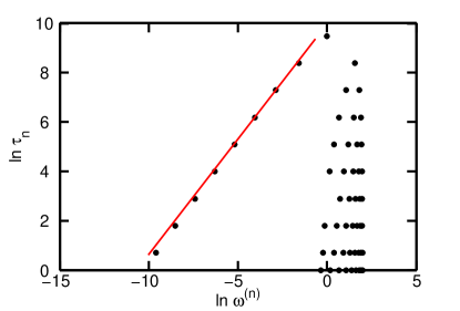
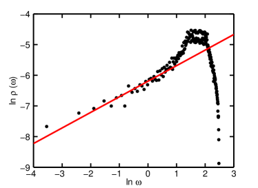
Figure 1: (Color online) The degeneracies, τnsubscript𝜏𝑛\tau_{n}, of the distinct eigenvalues ω(n)superscript𝜔𝑛\omega^{(n)} for the Cayley tree (with branching number b=3𝑏3b=3), drawn for r=9𝑟9r=9 generations. The smallest nonzero eigenvalue tends to zero as brsuperscript𝑏𝑟b^{-r}. We do not display ω1=0subscript𝜔10\omega_{1}=0. The degeneracies fall on a straight line with unit slope (red in color) in this log-log plot. Nevertheless, the spectral density is zero almost everywhere within the ω<1𝜔1\omega<1 domain, and the exponent β𝛽\beta, defined via ρ(ω)ωβsimilar-to𝜌𝜔superscript𝜔𝛽\rho(\omega)\sim\omega^{\beta} for small ω𝜔\omega is equal to zero. See text.

It is easy to show (from Eqs.(12,22) that if the spectral density exhibits a power law behaviour, with ρ(ω)ωβsimilar-to𝜌𝜔superscript𝜔𝛽\rho(\omega)\sim\omega^{\beta} for small ω𝜔\omega, then the nontrivial exponents p1subscript𝑝1p_{1} and ϕ2subscriptitalic-ϕ2\phi_{2}, within the context, respectively, of scaling the maximum eigenvalue or the number of modes, are related to β𝛽\beta via

ϕ2=1/(1+β)p1=1+β.formulae-sequencesubscriptitalic-ϕ211𝛽subscript𝑝11𝛽\phi_{2}=1/(1+\beta)\;\;\;\;p_{1}=1+\beta\;\;. (27)

From β0𝛽0\beta\geq 0, we are ensured that ϕ21subscriptitalic-ϕ21\phi_{2}\leq 1 and p11subscript𝑝11p_{1}\geq 1, and finally,

α=1βδ=(2+β)/β.formulae-sequence𝛼1𝛽𝛿2𝛽𝛽\alpha=1-\beta\;\;\;\;\delta=(2+\beta)/\beta\;\;. (28)

In terms of the spectral dimension Bianconi2010 d~2(1+β)~𝑑21𝛽\tilde{d}\equiv 2(1+\beta) one gets.

α=4d~2δ=d~+2d~2,formulae-sequence𝛼4~𝑑2𝛿~𝑑2~𝑑2\alpha=\frac{4-\tilde{d}}{2}\;\;\;\;\delta=\frac{\tilde{d}+2}{\tilde{d}-2}\;\;, (29)

so that for the Gaussian model, the exponents depend solely on the spectral dimension. A comparison with the exactly known Gaussian exponents in spatial dimension d𝑑d  Huang ; Goldenfeld shows that here the spectral dimension has taken on the role of the spatial dimension.

III Spectral RG for some Deterministic Networks

In this section we present numerical and semi-analytical results for the spectral renormalization of the Gaussian model on the Cayley tree and the diamond lattice. In the Appendix, the analogous computations for the square and cubic lattices are presented for comparison.

III.1 Gaussian model on the Cayley tree

An inspection of Fig. 1 shows that the spectral density of the graph Laplacian for the Cayley tree can be written as

ρ(ω)=n=1rτnδ(ωω(n)),𝜌𝜔superscriptsubscript𝑛1𝑟subscript𝜏𝑛𝛿𝜔superscript𝜔𝑛\rho(\omega)=\sum_{n=1}^{r}\tau_{n}\delta(\omega-\omega^{(n)})\;\;, (30)

where ω(n)superscript𝜔𝑛\omega^{(n)} and τn=τ(ω(n))ω(n)subscript𝜏𝑛𝜏superscript𝜔𝑛proportional-tosuperscript𝜔𝑛\tau_{n}=\tau(\omega^{(n)})\propto\omega^{(n)} are the n=1,2,𝑛12n=1,2,\ldotsth distinct eigenvalues and their degeneracies in the interval 0<ω<ω0𝜔superscript𝜔0<\omega<\omega^{*}, where ωsuperscript𝜔\omega^{*} is the value at which τ(ω)𝜏𝜔\tau(\omega) is maximum.

We see that, for branching number b𝑏b and n>1𝑛1n>1,

τn=bn2(b1)subscript𝜏𝑛superscript𝑏𝑛2𝑏1\tau_{n}=b^{n-2}(b-1) (31)

and

ω(n)anb(rn+2),similar-to-or-equalssuperscript𝜔𝑛subscript𝑎𝑛superscript𝑏𝑟𝑛2\omega^{(n)}\simeq a_{n}b^{-(r-n+2)}\;\;, (32)

where clearly

τn[ω(n)]ξ.proportional-tosubscript𝜏𝑛superscriptdelimited-[]superscript𝜔𝑛𝜉\tau_{n}\propto[\omega^{(n)}]^{\xi}\;\;. (33)

In fact we find ξ=1𝜉1\xi=1. The coefficients ansubscript𝑎𝑛a_{n} tend to a constant, with an+1/an1+c1exp(c2n)similar-tosubscript𝑎𝑛1subscript𝑎𝑛1subscript𝑐1subscript𝑐2𝑛a_{n+1}/a_{n}\sim 1+{c_{1}}\exp(c_{2}n) for rn1much-greater-than𝑟𝑛1r-n\gg 1, with c1subscript𝑐1c_{1} of the order of e(r2)1much-less-thansuperscript𝑒𝑟21e^{-(r-2)}\ll 1 and c2O(1)similar-tosubscript𝑐2𝑂1c_{2}\sim O(1). Since we are interested in the small ω𝜔\omega region of the spectrum we will henceforth treat the ansubscript𝑎𝑛a_{n} as constants. The number of eigenvalues within the interval ω<1𝜔1\omega<1 is br1Nr/bsimilar-to-or-equalsabsentsuperscript𝑏𝑟1similar-tosubscript𝑁𝑟𝑏\simeq b^{r-1}\sim N_{r}/b.

To find the spectral dimension, i.e., the scaling form of the spectral density, let us consider going from the discrete sum over n𝑛n to a continuous integral. Defining the continuous variable x𝑥x via ω(n)exp(xlnb)proportional-tosuperscript𝜔𝑛𝑥𝑏\omega^{(n)}\propto\exp(x\,\ln b) and using Eq. (33),

nτn𝑑xexp(ξxlnb).proportional-tosubscript𝑛subscript𝜏𝑛differential-d𝑥𝜉𝑥𝑏\sum_{n}\tau_{n}\propto\int dx\exp(\xi x\;\ln b)\;\;. (34)

Making the change of variables ω(x)=exp(xlnb)𝜔𝑥𝑥𝑏\omega(x)=\exp(x\,\ln b), we get dω=lnbexp(xlnb)dx𝑑𝜔𝑏𝑥𝑏𝑑𝑥d\omega=\ln b\exp(x\;\ln b)dx or

dx=dωωlnb.𝑑𝑥𝑑𝜔𝜔𝑏dx=\frac{d\omega}{\omega\;\ln b}\;\;. (35)

Thus

nτndωωξωlnb=1lnbωξ1𝑑ω.subscript𝑛subscript𝜏𝑛𝑑𝜔superscript𝜔𝜉𝜔𝑏1𝑏superscript𝜔𝜉1differential-d𝜔\sum_{n}\tau_{n}\to\int\frac{d\omega\;\omega^{\xi}}{\omega\;\ln b}=\frac{1}{\ln b}\int\omega^{\xi-1}d\omega\;\;. (36)

This yields ρ(ω)ωβsimilar-to𝜌𝜔superscript𝜔𝛽\rho(\omega)\sim\omega^{\beta} with β=ξ1𝛽𝜉1\beta={\xi-1}, and since we have found ξ=1𝜉1\xi=1, we see that β=0𝛽0\beta=0 in the region ω<1𝜔1\omega<1. Notice that the spectral density (and therefore also the spectral dimension) do not depend on the branching number b𝑏b.

It is straightforward to directly compute the renormalization group eigenvalues from a knowledge of the structure of the discrete eigenvalue spectrum. Choosing B=bkBk𝐵superscript𝑏𝑘subscript𝐵𝑘B=b^{k}\equiv B_{k}, we have, for the rescaling factors,

σ1V(Bk)=Nn=0r1kτn=Bϕ1,subscriptsuperscript𝜎V1subscript𝐵𝑘𝑁superscriptsubscript𝑛0𝑟1𝑘subscript𝜏𝑛superscript𝐵subscriptitalic-ϕ1\ {\sigma^{\rm V}_{1}(B_{k})}=\frac{N}{\sum_{n=0}^{r-1-k}\tau_{n}}=B^{\phi_{1}}\;\;, (37)

and

σ1V(Bk)σ2V(Bk)=Nω¯n=0r1kτnω(n)Bϕ1+ϕ2,subscriptsuperscript𝜎V1subscript𝐵𝑘superscriptsubscript𝜎2Vsubscript𝐵𝑘𝑁¯𝜔superscriptsubscript𝑛0𝑟1𝑘subscript𝜏𝑛superscript𝜔𝑛proportional-tosuperscript𝐵subscriptitalic-ϕ1subscriptitalic-ϕ2\ \sigma^{\rm V}_{1}(B_{k})\sigma_{2}^{\rm V}(B_{k})=\;\frac{N\overline{\omega}}{\sum_{n=0}^{r-1-k}\tau_{n}\omega^{(n)}}\propto B^{\phi_{1}+\phi_{2}}\;\;, (38)

where we have set, an=const.subscript𝑎𝑛consta_{n}={\rm const.}.

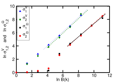
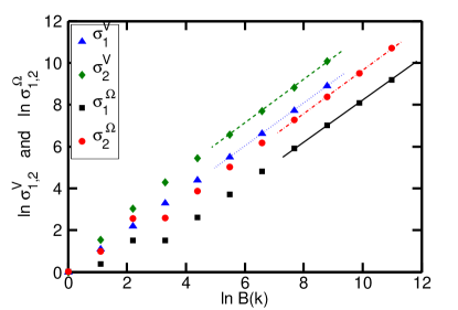
Doing the sums for r1much-greater-than𝑟1r\gg 1, 1k<rmuch-less-than1𝑘𝑟1\ll k<r, (i.e. in the small ω𝜔\omega region), we find ϕ1=ϕ2=1subscriptitalic-ϕ1subscriptitalic-ϕ21\phi_{1}=\phi_{2}=1. The numerically obtained scaling behavior of σ1Vsubscriptsuperscript𝜎V1\sigma^{\rm V}_{1} and σ2Vsuperscriptsubscript𝜎2V\sigma_{2}^{\rm V}, as well as σ1Ωsubscriptsuperscript𝜎Ω1\sigma^{\Omega}_{1} and σ2Ωsuperscriptsubscript𝜎2Ω\sigma_{2}^{\Omega} are shown in Fig. 2, and are in agreement with our approximate analytical result. The critical exponents are given in Table 1.
Refer to caption
Figure 2: (Color online) Rescaling factors σiVsubscriptsuperscript𝜎V𝑖\sigma^{\rm V}_{i}, and σiΩsubscriptsuperscript𝜎Ω𝑖\sigma^{\Omega}_{i}, i=1,2𝑖12i=1,2 for the Cayley tree with branching number b=3𝑏3b=3. See text, Eqs.(11,12,20,22). The scale factor is chosen as B(k)=bk1𝐵𝑘superscript𝑏𝑘1B(k)=b^{k-1}. The linear fits are to the last four points for each set. The exponents are found to be ϕ1=1.00subscriptitalic-ϕ11.00\phi_{1}=1.00, ϕ2=1.03±0.04subscriptitalic-ϕ2plus-or-minus1.030.04\phi_{2}=1.03\pm 0.04, p1=1,p2=1.01±0.01formulae-sequencesubscript𝑝11subscript𝑝2plus-or-minus1.010.01p_{1}=1,\;\;p_{2}=1.01\pm 0.01. The critical exponents are given in Table 1.

III.2 Gaussian model on the diamond lattice

We next consider a hierarchical lattice, sometimes also known as the diamond lattice diamond . The zeroth generation consists of two nodes connected by an edge; at the first iteration the edge is replaced by a rhombus with the two new nodes making up the first generation, and the network is constructed by iteratively replacing each edge of a rhombus by yet another rhombus. Indexing the different generations by k=0,,r𝑘0𝑟k=0,\ldots,r, the total number of nodes is Nr=2(1+k=0r14k)subscript𝑁𝑟21superscriptsubscript𝑘0𝑟1superscript4𝑘N_{r}=2(1+\sum_{k=0}^{r-1}4^{k}), the number added at each generation is NkNk1=22k1subscript𝑁𝑘subscript𝑁𝑘1superscript22𝑘1N_{k}-N_{k-1}=2^{2k-1} for any k1𝑘1k\geq 1.

After r𝑟r iterations, the nodes belonging the k𝑘kth generation have degrees dksubscript𝑑𝑘d_{k}, where d0=d1=2rsubscript𝑑0subscript𝑑1superscript2𝑟d_{0}=d_{1}=2^{r} and dk=2rk+1,subscript𝑑𝑘superscript2𝑟𝑘1d_{k}=2^{r-k+1}, for 1<kr1𝑘𝑟1<k\leq r. This leads to an overall scale free degree distribution with γ=2𝛾2\gamma=2. On the other hand, embedding the lattice in a metric space and regarding the iterations as a fine-graining operation GriffithsandKaufman leads to a multifractal degree distribution over the lattice Erzan1997 .
Refer to caption
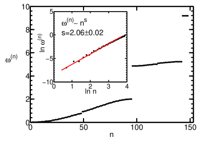
Figure 3: (Color online) The distinct eigenvalues ω(n)superscript𝜔𝑛\omega^{(n)} of the graph Laplacian on the diamond lattice plotted against n𝑛n. The inset shows the scaling behavior in the small ω(n)superscript𝜔𝑛\omega^{(n)} region.
Refer to caption
Figure 4: Spectral distribution for the diamond lattice, for r=7𝑟7r=7 generations, on a log-log scale. Families of eigenvalues with degeneracies τj=kj4ksubscript𝜏𝑗superscriptsubscript𝑘𝑗superscript4𝑘\tau_{j}=\sum_{k}^{j}4^{k} can be seen as horizontal sets of points.
Refer to caption
Figure 5: (Color online) The numerically calculated rescaling factors for the diamond lattice. The scale factors have been chosen as B(k)=22k𝐵𝑘superscript22𝑘B(k)=2^{2k} and 1k<r+11\leq k<\leq r+1 for σ1V,σ2Vsuperscriptsubscript𝜎1Vsuperscriptsubscript𝜎2V\sigma_{1}^{\rm V},\;\;\sigma_{2}^{\rm V} and 1kr+21𝑘𝑟21\leq k\leq r+2 for σ1Ω,σ2Ωsuperscriptsubscript𝜎1Ωsuperscriptsubscript𝜎2Ω\sigma_{1}^{\Omega},\;\;\sigma_{2}^{\Omega}, for a total number of generations r=7𝑟7r=7. The linear fits are to the last four points for each set. We get ϕ1=1subscriptitalic-ϕ11\phi_{1}=1, ϕ2=1.01±0.03subscriptitalic-ϕ2plus-or-minus1.010.03\phi_{2}=1.01\pm 0.03, p1=0.97±0.04subscript𝑝1plus-or-minus0.970.04p_{1}=0.97\pm 0.04 and p2=1.06±0.02subscript𝑝2plus-or-minus1.060.02p_{2}=1.06\pm 0.02. The critical exponents are summarized in Table 1.

We are interested in the region 0ω20𝜔20\leq\omega\leq 2 where ω(n+1)ω(n)0delimited-⟨⟩superscript𝜔𝑛1superscript𝜔𝑛0\langle\omega^{(n+1)}-\omega^{(n)}\rangle\equiv\ell\to 0 as 4rsuperscript4𝑟4^{-r}. We find that the degeneracies of the distinct eigenvalues ω(n)superscript𝜔𝑛\omega^{(n)} obey a scaling relation ω(n)nssimilar-tosuperscript𝜔𝑛superscript𝑛𝑠\omega^{(n)}\sim n^{s} with s=2.06±0.02𝑠plus-or-minus2.060.02s={2.06}\pm 0.02 for small n𝑛n (Fig. 3). The degeneracies τnsubscript𝜏𝑛\tau_{n} are organized in triplets, 𝐓j={1,2,τ(j)}subscript𝐓𝑗12𝜏𝑗\mathbf{T}_{j}=\{1,2,\tau(j)\}, with τ(j)𝜏𝑗\tau(j) being defined now as the j𝑗jth distinct element of the series 1,5,21,15211,5,21, etc. given by τ(j+1)=4τ(j)+1𝜏𝑗14𝜏𝑗1\tau(j+1)=4\tau(j)+1, or τ(j)=k=0j4k4j𝜏𝑗superscriptsubscript𝑘0𝑗superscript4𝑘similar-tosuperscript4𝑗\tau(j)=\sum_{k=0}^{j}4^{k}\sim 4^{j}, for 0jr10𝑗𝑟10\leq j\leq r-1. The spectral distribution is naturally embedded in the real numbers and has a multifractal structure, which is generated by the replacements 𝐓1{𝐓1,𝐓2,𝐓1}subscript𝐓1subscript𝐓1subscript𝐓2subscript𝐓1\mathbf{T}_{1}\to\{\mathbf{T}_{1},\mathbf{T}_{2},\mathbf{T}_{1}\} and, for j2𝑗2j\geq 2, 𝐓j𝐓j+1subscript𝐓𝑗subscript𝐓𝑗1\mathbf{T}_{j}\to\mathbf{T}_{j+1} at each iteration.

The spectral distribution for the diamond lattice, plotted on a log-log scale, is shown in Fig. 4, with the initial ω𝜔\omega values for each j𝑗jth family being given by ωinit(j)4jproportional-tosubscript𝜔init𝑗superscript4𝑗\omega_{\rm init}(j)\propto 4^{j} obeying the scaling relation τ(j)ωinit(j)proportional-to𝜏𝑗subscript𝜔init𝑗\tau(j)\propto\omega_{\rm init}(j), so that the envelope of the distribution is qualitatively the same as that of the Cayley tree, Fig. 1.

The complexity of this spectral distribution is tamed by the rescaling factors σ1subscript𝜎1\sigma_{1} and σ2subscript𝜎2\sigma_{2}. It should be noted that σ11nnBτnsimilar-tosuperscriptsubscript𝜎11superscriptsubscript𝑛subscript𝑛𝐵subscript𝜏𝑛\sigma_{1}^{-1}\sim\sum_{n}^{n_{B}}\tau_{n} and σ11σ21nnBω(n)τnsimilar-tosuperscriptsubscript𝜎11superscriptsubscript𝜎21superscriptsubscript𝑛subscript𝑛𝐵subscript𝜔𝑛subscript𝜏𝑛\sigma_{1}^{-1}\sigma_{2}^{-1}\sim\sum_{n}^{n_{B}}\omega_{(n)}\tau_{n} (with nB=r1ksubscript𝑛𝐵𝑟1𝑘n_{B}=r-1-k for B(k)=4k𝐵𝑘superscript4𝑘B(k)=4^{k}) are, respectively the (truncated) zeroth and 1st moments of the multifractal spectral distribution described above. These integrated quantities smooth out the singular nature of the distribution itself, and yield simple scaling law for large B𝐵B (small ω𝜔\omega), the relevant regime for the critical behavior.

In Fig.(5) σ1Vsubscriptsuperscript𝜎V1\sigma^{\rm V}_{1}, σ2Vsubscriptsuperscript𝜎V2\sigma^{\rm V}_{2}, σ1Ωsubscriptsuperscript𝜎Ω1\sigma^{\Omega}_{1} and σ2Ωsubscriptsuperscript𝜎Ω2\sigma^{\Omega}_{2}, are calculated numerically, again with a set of scale factors B(k)=4k𝐵𝑘superscript4𝑘B(k)=4^{k}, in keeping with the discrete scaling symmetry of the lattice. The exponents are given in in Table 1. The numerically computed values of the critical exponents are in agreement with the scaling behavior (β=0𝛽0\beta=0, i.e., d~=2~𝑑2{\tilde{d}}=2) which one may read off from the envelope of the spectral distribution (Fig.4).

Table 1: Exponents of the spectral density, the rescaling factors and critical exponents obtained for the Gaussian model on spatial and non-spatial networks. The first set of exponents are obtained by the method of scaling the total number of modes, and the second set via scaling the upper cutoff for the eigenvalues. The values for δ𝛿\delta that are larger than the inverse of the error bars around zero have been shown as \infty. The Gaussian model yields identical results on the square lattice, the Cayley tree and the diamond lattice, which all have spectral dimension d~=2~𝑑2\tilde{d}=2. The exact Gaussian values are indicated with the subscript G𝐺G. See text for definitions.
Network β𝛽\beta ϕ1subscriptitalic-ϕ1\phi_{1} ϕ2subscriptitalic-ϕ2\phi_{2} α𝛼\alpha δ𝛿\delta   p1subscript𝑝1p_{1}   p2subscript𝑝2p_{2}    α𝛼\alpha δ𝛿\delta αGsubscript𝛼𝐺\alpha_{G} δGsubscript𝛿𝐺\delta_{G}
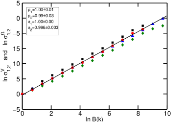
Square 0.00±0.02plus-or-minus0.000.020.00\pm 0.02 111 0.996±0.003plus-or-minus0.9960.0030.996\pm 0.003 111 \infty 1.00±0.01plus-or-minus1.000.011.00\pm 0.01 0.99±0.03plus-or-minus0.990.030.99\pm 0.03 1.00±0.03plus-or-minus1.000.031.00\pm 0.03 \infty 1 \infty
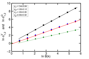
Cubic 0.5±0.1plus-or-minus0.50.10.5\pm 0.1 111 0.66±0.05plus-or-minus0.660.050.66\pm 0.05 0.48±0.12plus-or-minus0.480.120.48\pm 0.12 4.88±0.25plus-or-minus4.880.254.88\pm 0.25 1.49±0.02plus-or-minus1.490.021.49\pm 0.02 0.98±0.05plus-or-minus0.980.050.98\pm 0.05 0.48±0.05plus-or-minus0.480.050.48\pm 0.05 4.8±0.4plus-or-minus4.80.44.8\pm 0.4 1/2121/2 5
Cayley3 1.03±0.04plus-or-minus1.030.041.03\pm 0.04 111 1.03±0.04plus-or-minus1.030.041.03\pm 0.04 1.03±0.04plus-or-minus1.030.041.03\pm 0.04 \infty 111 1.01±0.01plus-or-minus1.010.011.01\pm 0.01 0.99±0.01plus-or-minus0.990.010.99\pm 0.01 \infty 1 \infty
Cayley5 1.06±0.09plus-or-minus1.060.091.06\pm 0.09 111 1.06±0.09plus-or-minus1.060.091.06\pm 0.09 1.06±0.09plus-or-minus1.060.091.06\pm 0.09 \infty 111 1.05±0.05plus-or-minus1.050.051.05\pm 0.05 0.95±0.05plus-or-minus0.950.050.95\pm 0.05 \infty 1 \infty
Diamond 1.01±0.03plus-or-minus1.010.031.01\pm 0.03 111 1.01±0.03plus-or-minus1.010.031.01\pm 0.03 1.01±0.03plus-or-minus1.010.031.01\pm 0.03 \infty 0.97±0.04plus-or-minus0.970.040.97\pm 0.04 1.06±0.07plus-or-minus1.060.071.06\pm 0.07 1.09±0.11plus-or-minus1.090.111.09\pm 0.11 \infty 1 \infty

III.3 Recovering the Mean Field exponents

Goldenfeld Goldenfeld discusses the anomaly of obtaining non-classical (non-mean field) values for the critical exponents of the Gaussian model, which is based on a Landau expansion (see Eq.(1)) and points out that the anomaly can be understood in terms of the dangerous irrelevant field v0subscript𝑣0v_{0}. We may repeat the argument in the present case, using the scaling relation in Eq. (16) with a third scaling field, v𝑣v, so that f=Bxf(BYt(x)t,BYh(x)h,BYv(x)v)𝑓superscript𝐵𝑥superscript𝑓superscript𝐵subscript𝑌𝑡𝑥𝑡superscript𝐵subscript𝑌𝑥superscript𝐵subscript𝑌𝑣𝑥𝑣f=B^{-x}f^{\prime}(B^{Y_{t}(x)}t,B^{Y_{h}(x)}h,B^{Y_{v}(x)}v), yielding

m(0,h,v)=h[Yh(x)+x]/Yh(x)(vhYv/Yh),𝑚0𝑣superscriptdelimited-[]subscript𝑌𝑥𝑥subscript𝑌𝑥𝑣superscriptsubscript𝑌𝑣subscript𝑌m(0,h,v)=h^{[-Y_{h}(x)+x]/Y_{h}(x)}{\mathcal{M}}(vh^{-Y_{v}/Y_{h}})\;\;, (39)

for the magnetization on the critical isotherm. Here x=1𝑥1x=1 or x=p1=1+β𝑥subscript𝑝11𝛽x=p_{1}=1+\beta depending on whether we scale the number of modes (Section II.A) or the maximum eigenvalue (Section II.B), respectively. We will require that Yv1βproportional-tosubscript𝑌𝑣1𝛽Y_{v}\propto 1-\beta, in analogy with setting yv4dproportional-tosubscript𝑦𝑣4𝑑y_{v}\propto 4-d in Euclidean space. The Landau expansion gives m(0,h,v)(h/v)1/3proportional-to𝑚0𝑣superscript𝑣13m(0,h,v)\propto(h/v)^{1/3}; therefore one takes Goldenfeld the scaling function (v)v1/3similar-to𝑣superscript𝑣13{\mathcal{M}}(v)\sim v^{-1/3} in the limit of small hh. Eq.(39) then gives

1+xYh(x)+13Yv(x)Yh(x)=1δ.1𝑥subscript𝑌𝑥13subscript𝑌𝑣𝑥subscript𝑌𝑥1𝛿-1+\frac{x}{Y_{h}(x)}+\frac{1}{3}\frac{Y_{v}(x)}{Y_{h}(x)}=\frac{1}{\delta}\;\;. (40)

For x=1+β𝑥1𝛽x=1+\beta, one has Yh=(2+β)/2subscript𝑌2𝛽2Y_{h}=(2+\beta)/2, Yv=1βsubscript𝑌𝑣1𝛽Y_{v}=1-\beta. For x=1𝑥1x=1, Yh=(2+β)/[2(1+β)]subscript𝑌2𝛽delimited-[]21𝛽Y_{h}=(2+\beta)/[2(1+\beta)] and one must take Yv=(1β)/(1+β)subscript𝑌𝑣1𝛽1𝛽Y_{v}=(1-\beta)/(1+\beta). In either case, β𝛽\beta cancels out of the final result, yielding the mean field value for δ𝛿\delta. One may similarly show that keeping v0subscript𝑣0v_{0} in the calculation and using the Landau expansion for h=00h=0 to get mr0/v0proportional-to𝑚subscript𝑟0subscript𝑣0m\propto\sqrt{-r_{0}/v_{0}} gives the order parameter exponent βmsubscript𝛽𝑚\beta_{m} to be 1/2121/2, from which one may derive α=0𝛼0\alpha=0 using the scaling relation βm(1+δ)=2αsubscript𝛽𝑚1𝛿2𝛼\beta_{m}(1+\delta)=2-\alpha.

III.4 Square and cubic lattices

For completeness, we have also computed the spectral densities of the square and cubic lattices, and their rescaling factors. The Laplace eigenvalues for the square and cubic lattices are analytically given by

ω𝐪=4j=1dsin2(qj2)subscript𝜔𝐪4superscriptsubscript𝑗1𝑑superscript2subscript𝑞𝑗2\omega_{\mathbf{q}}=4\sum_{j=1}^{d}\sin^{2}\left(\frac{q_{j}}{2}\right) (41)

where we have indexed the eigenvalues by the wave vector, the lattice spacing is unity, d𝑑d is the Euclidean dimension and qj=(πnjN1/d)subscript𝑞𝑗𝜋subscript𝑛𝑗superscript𝑁1𝑑q_{j}=(\pi n_{j}\,N^{-1/d}) are the Cartesian components of 𝐪𝐪\mathbf{q}. In the limit of small q=𝐪𝑞norm𝐪q=\|{\mathbf{q}}\|, ω𝐪q2similar-to-or-equalssubscript𝜔𝐪superscript𝑞2\omega_{\mathbf{q}}\simeq q^{2}. Then the spectral density is ρ(ω)ωβproportional-to𝜌𝜔superscript𝜔𝛽\rho(\omega)\propto\omega^{\beta} with β=d/21𝛽𝑑21\beta={d/2}-1.

The numerical results for the non-trivial scaling exponents and for α𝛼\alpha and δ𝛿\delta are given in Table 1. The plots of the spectral density and rescaling factors are provided in the Appendix. It is instructive to compare the accuracy obtainable from the rescaling factors as opposed to the spectral densities themselves, which converge very slowly, in the small ω𝜔\omega region, to their thermodynamic limits.

IV Comparison with conventional methods

In this section we would like to check our SRG results against conventional methods which we here adapt to non-spatial lattices, namely, exact summation of the leading term in the specific heat, obtained by differentialting Eq. (8), and finite size scaling (FSS) by the number of nodes of the lattice, instead of the linear size of the system.

IV.1 Exact Enumeration

For the Gaussian model, the specific heat can be explicitly calculated to leading order as,

ch12Nμ=1N1(r0+ωμ)2=1Nn=0r1τn[t+ω(n)]2.proportional-tosubscript𝑐12𝑁superscriptsubscript𝜇1𝑁1superscriptsubscript𝑟0subscript𝜔𝜇21𝑁superscriptsubscript𝑛0𝑟1subscript𝜏𝑛superscriptdelimited-[]𝑡superscript𝜔𝑛2c_{h}\propto\frac{1}{2N}\sum_{\mu=1}^{N}\frac{1}{(r_{0}+\omega_{\mu})^{2}}\\ =\frac{1}{N}\sum_{n=0}^{r-1}{\tau_{n}\over[t+\omega^{(n)}]^{2}}\;\;. (42)

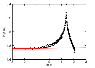
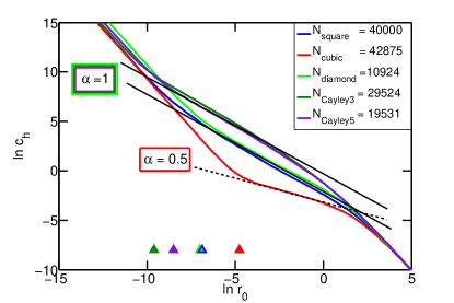
The results for the Cayley tree, the diamond lattice, and square and cubic lattices, are shown in Fig.(6). The critical scaling behaviour of chsubscript𝑐c_{h} is obtained for r0subscript𝑟0r_{0} between the first nonzero Laplace eigenvalue and the van Hove singularity in the Laplacian spectral density (which falls near unity) and yields the critical exponent α𝛼\alpha in agreement with the SRG results in Table 1.
Refer to caption
Figure 6: (Color online) Specific heat exponent α𝛼\alpha obtained from Eq.(42), for the Cayley tree with branching numbers b=3, 5𝑏35b=3,\;5 (indistinguishable in graph) and the diamond, square and cubic lattices. The legend indicates the size of the different lattices. The positions of the first nonzero eigenvalues of the graph Laplacian are indicated by triangles with colors that match the curves, and mark the onset of the scaling region. The slope of the tangent lines yield α=1𝛼1\alpha=1 for all except the cubic lattice, which has α=0.5𝛼0.5\alpha=0.5.

IV.2 Finite Size Scaling for non-spatial lattices

In order to estimate possible errors due to the finiteness of the lattices considered, an FSS analysis adapted to non-spatial lattices was performed for the example of the Cayley tree. The size-dependent relevant effective “field” in this case is N1superscript𝑁1N^{-1}, in place of the linear size of the spatial lattice Goldenfeld .

The specific heat should then scale as

ch(t,N1)N2Y1={const.,x<1x12Y,x>1.subscript𝑐𝑡superscript𝑁1superscript𝑁2𝑌1casesconst𝑥1superscript𝑥12𝑌𝑥1\frac{c_{h}(t,N^{-1})}{N^{2Y-1}}=\begin{cases}{\rm const.},&\mbox{$x<1$}\\ x^{1-2Y},&\mbox{$x>1$}.\end{cases} (43)

where x=t(1/Y)N𝑥superscript𝑡1𝑌𝑁x=t^{(1/Y)}N. Plotting N(2Y1)chsuperscript𝑁2𝑌1subscript𝑐N^{-(2Y-1)}c_{h} vs. Nt𝑁𝑡Nt, we find Y=1𝑌1Y=1, with a satisfactory collapse for r=3,,7𝑟37r=3,\ldots,7. We can show that α=2Y1𝛼2superscript𝑌1\alpha=2-Y^{-1} and our SRG result for α𝛼\alpha is confirmed.

For the Cayley tree, the same result may be obtained by substituting the approximate analytic results for τnsubscript𝜏𝑛\tau_{n} and ω(n)superscript𝜔𝑛\omega^{(n)} from Eqs.(32,33) into Eq. (42). Noticing that brNrsimilar-tosuperscript𝑏𝑟subscript𝑁𝑟b^{r}\sim N_{r}, one gets, after multiplying and dividing the RHS by Nr2superscriptsubscript𝑁𝑟2N_{r}^{2} and simplifying,

chNrb1b2n=0r1bn(Nrt+bn)2.similar-to-or-equalssubscript𝑐subscript𝑁𝑟𝑏1superscript𝑏2superscriptsubscript𝑛0𝑟1superscript𝑏𝑛superscriptsubscript𝑁𝑟𝑡superscript𝑏𝑛2\frac{c_{h}}{N_{r}}\simeq\frac{b-1}{b^{2}}\sum_{n=0}^{r-1}\frac{b^{n}}{(N_{r}\,t+b^{n})^{2}}\;\;. (44)

The RHS is only a function of Nrtsubscript𝑁𝑟𝑡N_{r}\,t and approaches a constant for Nrt<1subscript𝑁𝑟𝑡1N_{r}t<1. Going over to an integral immediately gives the result that ch(Nrt)1similar-tosubscript𝑐superscriptsubscript𝑁𝑟𝑡1c_{h}\sim(N_{r}\,t)^{-1} for Nrt>1subscript𝑁𝑟𝑡1N_{r}\,t>1.

V Including the ψ4superscript𝜓4\psi^{4} interactions

In this section we will add a ψ4superscript𝜓4\psi^{4} term (Eq.1) to the Gaussian Hamiltonian and treat this system on the Cayley tree and the diamond lattice. This interaction term leads to couplings between different fluctuation modes, and the precise nature of the eigenvectors come to play an important role.

The Ising model exhibits Mean Field critical behavior on the Bethe Lattice (Cayley tree in the infinite limit) Eggarter ; CJThompson , therefore we should expect to find that on this network, the Gaussian fixed point is stable with respect to the inclusion of a ψ4superscript𝜓4\psi^{4} coupling. However, on the diamond lattice, we would expect the emergence of a non-Gaussian fixed point as well, since the Ising model on the diamond lattice undergoes an order-disorder phase transition with non-trivial exponents. KaufmanandGriffiths ; GriffithsandKaufman

The interaction term Hint=v0iψ4(i)subscript𝐻intsubscript𝑣0subscript𝑖superscript𝜓4𝑖H_{\rm int}=v_{0}\sum_{i}\psi^{4}(i) in the Hamiltonian (see Eq. 1) can be expanded explicitly in terms of the eigenvectors of the graph Laplacian on an arbitrary network, as

Hint=v01,2,3,4ψ^1ψ^2ψ^3ψ^4Φ(1,2,3,4),subscript𝐻intsubscript𝑣0subscript1234subscript^𝜓1subscript^𝜓2subscript^𝜓3subscript^𝜓4Φ1234H_{\rm int}=v_{0}\sum_{1,2,3,4}\hat{\psi}_{1}\hat{\psi}_{2}\hat{\psi}_{3}\hat{\psi}_{4}\;\Phi(1,2,3,4)\;\;, (45)

where, for brevity, we have written {1,2,3,4}1234\{1,2,3,4\} instead of {μ1,μ2,μ3,μ4}subscript𝜇1subscript𝜇2subscript𝜇3subscript𝜇4\{\mu_{1},\mu_{2},\mu_{3},\mu_{4}\} and we have defined the 4-vertex

Φ(1,2,3,4)=iNu1(i)u2(i)u3(i)u4(i).Φ1234superscriptsubscript𝑖𝑁subscript𝑢1𝑖subscript𝑢2𝑖subscript𝑢3𝑖subscript𝑢4𝑖\Phi(1,2,3,4)=\sum_{i}^{N}u_{1}(i)u_{2}(i)u_{3}(i)u_{4}(i)\;\;\;. (46)

Here uμ(i)subscript𝑢𝜇𝑖u_{\mu}(i) is the i𝑖ith element of the eigenvector 𝐮μsubscript𝐮𝜇\mathbf{u}_{\mu} of the graph Laplacian.

On a periodic lattice where the eigenvectors are the harmonic functions uμ(j)=N1/2exp(i𝐤μ𝐱j)subscript𝑢𝜇𝑗superscript𝑁12𝑖subscript𝐤𝜇subscript𝐱𝑗u_{\mu}(j)=N^{-1/2}\exp(i\mathbf{k}_{\mu}\cdot\mathbf{x}_{j}) and ωμ=𝐤μ2subscript𝜔𝜇superscriptnormsubscript𝐤𝜇2\omega_{\mu}=\|\mathbf{k}_{\mu}\|^{2}, one immediately has

Φ(1,2,3,4)=δ(d)(𝐤1+𝐤2+𝐤3+𝐤4),Φ1234superscript𝛿𝑑subscript𝐤1subscript𝐤2subscript𝐤3subscript𝐤4\Phi(1,2,3,4)=\delta^{(d)}(\mathbf{k}_{1}+\mathbf{k}_{2}+\mathbf{k}_{3}+\mathbf{k}_{4})\;\;, (47)

where, in the thermodynamic limit δ(d)superscript𝛿𝑑\delta^{(d)} becomes the d𝑑d-dimensional Dirac δ𝛿\delta-function. In the case of an arbitrary network, a similar constraint is difficult to find in general, even with an analytical solution for the eigenvalues erzan ; Rojo ; Rabbiano ; Burda . In this paper we will avail ourselves of the numerically calculated eigenvectors for the respective lattices.

We now explicitly perform the scaling with respect to the maximum eigenvalue, by taking partial integrals in the partition function, over fields ψ^μsubscript^𝜓𝜇\hat{\psi}_{\mu} with μ>μB𝜇subscript𝜇𝐵\mu>\mu_{B}, with the Gaussian weight eH0>superscript𝑒superscriptsubscript𝐻0e^{-H_{0}^{>}}. We choose to define μBsubscript𝜇𝐵\mu_{B} as in Eq.(21), so that we are explicitly truncating the largest eigenvalue; however, truncating the number of modes gives parallel results for d~=2~𝑑2\tilde{d}=2. The superscripts >> and << have the same meaning as in Section II, i.e., H0>=12μ>μBN[r0+ωμ]ψ^μ2superscriptsubscript𝐻012superscriptsubscript𝜇subscript𝜇𝐵𝑁delimited-[]subscript𝑟0subscript𝜔𝜇superscriptsubscript^𝜓𝜇2H_{0}^{>}=\frac{1}{2}\sum_{\mu>\mu_{B}}^{N}[r_{0}+\omega_{\mu}]\hat{\psi}_{\mu}^{2}. Note that the functional eHintsuperscript𝑒subscript𝐻inte^{-H_{\rm int}} involves fields ψ^μsubscript^𝜓𝜇\hat{\psi}_{\mu} with μ𝜇\mu in both the lower and upper ranges with respect to the cutoff μBsubscript𝜇𝐵\mu_{B}, We obtain,

Z(r0,v0)=Z0>μ<μBdψ^μeH0<eHint0>.𝑍subscript𝑟0subscript𝑣0superscriptsubscript𝑍0superscriptsubscriptsubscriptproduct𝜇subscript𝜇𝐵𝑑subscript^𝜓𝜇superscript𝑒superscriptsubscript𝐻0superscriptsubscriptdelimited-⟨⟩superscript𝑒subscript𝐻int0Z(r_{0},v_{0})=Z_{0}^{>}\int_{-\infty}^{\infty}\prod_{\mu<\mu_{B}}d\hat{\psi}_{\mu}e^{-H_{0}^{<}}\langle e^{-H_{\rm int}}\rangle_{0}^{>}\;\;. (48)

The normalization factor is Z0>=μ>μBdψ^μeH0>superscriptsubscript𝑍0superscriptsubscriptsubscriptproduct𝜇subscript𝜇𝐵𝑑subscript^𝜓𝜇superscript𝑒superscriptsubscript𝐻0Z_{0}^{>}=\int_{-\infty}^{\infty}\prod_{\mu>\mu_{B}}d\hat{\psi}_{\mu}e^{-H_{0}^{>}}, and we have implicitly defined the expectation value,

𝒬0>=(Z0>)1μB<μ<Ndψ^μ𝒬eH0>.superscriptsubscriptdelimited-⟨⟩𝒬0superscriptsuperscriptsubscript𝑍01superscriptsubscriptsubscriptproductsubscript𝜇𝐵𝜇𝑁𝑑subscript^𝜓𝜇𝒬superscript𝑒superscriptsubscript𝐻0\langle{\cal Q}\rangle_{0}^{>}=(Z_{0}^{>})^{-1}\int_{-\infty}^{\infty}\prod_{\mu_{B}<\mu<N}d\hat{\psi}_{\mu}{\cal Q}e^{-H_{0}^{>}}\;\;\;. (49)

The perturbation up to second order in the coupling constant is obtained via a cumulant expansion,

exexe12[x2x2].similar-to-or-equalsdelimited-⟨⟩superscript𝑒𝑥superscript𝑒delimited-⟨⟩𝑥superscript𝑒12delimited-[]delimited-⟨⟩superscript𝑥2superscriptdelimited-⟨⟩𝑥2\langle e^{-x}\rangle\simeq e^{-\langle x\rangle}e^{\frac{1}{2}[\langle x^{2}\rangle-\langle x\rangle^{2}]}\;\;. (50)

V.1 First order terms

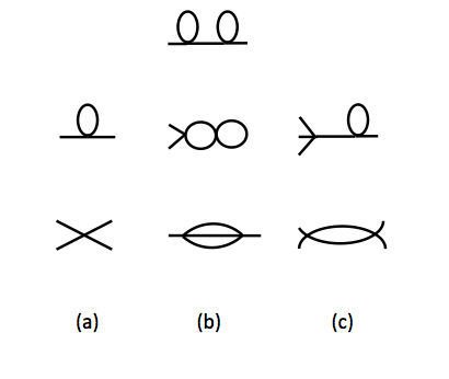
The different diagrams corresponding to the different terms in the perturbation expansion are given in Fig. 7. There are only two terms arising from the cumulant expansion to first order in v0subscript𝑣0v_{0}, and they are,

H2,1<=6v01,2<μBψ^1ψ^23>μBG(ω3,r0)Φ(1,2,3,3)superscriptsubscript𝐻216subscript𝑣0subscript12subscript𝜇𝐵subscript^𝜓1subscript^𝜓2subscript3subscript𝜇𝐵𝐺subscript𝜔3subscript𝑟0Φ1233H_{2,1}^{<}=6v_{0}\sum_{1,2<\mu_{B}}\hat{\psi}_{1}\hat{\psi}_{2}\sum_{3>\mu_{B}}G(\omega_{3},r_{0})\Phi(1,2,3,3) (51)

and

H4,1<=v01,2,3,4<μBψ^1ψ^2ψ^3ψ^4Φ(1,2,3,2).superscriptsubscript𝐻41subscript𝑣0subscript1234subscript𝜇𝐵subscript^𝜓1subscript^𝜓2subscript^𝜓3subscript^𝜓4Φ1232H_{4,1}^{<}=v_{0}\sum_{1,2,3,4<\mu_{B}}\hat{\psi}_{1}\hat{\psi}_{2}\hat{\psi}_{3}\hat{\psi}_{4}\Phi(1,2,3,2)\;\;. (52)

The Green’s function G(ω,r0)𝐺𝜔subscript𝑟0G(\omega,r_{0}) arises from the contraction of two fields with indices μ>μB𝜇subscript𝜇𝐵\mu>\mu_{B} and is defined via

ψ^μψ^μ0>=δμ,μ1ωμ+r0δμ,μG(ωμ,r0).superscriptsubscriptdelimited-⟨⟩subscript^𝜓𝜇subscript^𝜓superscript𝜇0subscript𝛿𝜇superscript𝜇1subscript𝜔𝜇subscript𝑟0subscript𝛿𝜇superscript𝜇𝐺subscript𝜔𝜇subscript𝑟0\langle\hat{\psi}_{\mu}\hat{\psi}_{\mu^{\prime}}\rangle_{0}^{>}=\delta_{\mu,\mu^{\prime}}\frac{1}{\omega_{\mu}+r_{0}}\equiv\delta_{\mu,\mu^{\prime}}G(\omega_{\mu},r_{0})\;\;. (53)

We see from Eqs. (51,52) that the couplings have acquired an eigenvector dependence, in a way similar to the case on periodic lattices. For the Cayley tree we can explicitly show that the 4-vertex Φ(μ1,μ2,μ3,μ3)Φsubscript𝜇1subscript𝜇2subscript𝜇3subscript𝜇3\Phi(\mu_{1},\mu_{2},\mu_{3},\mu_{3}) is nonzero only if its arguments are a) either equal pairwise, or b) one of them is equal to the constant vector and the remaining three equal to each other. In obvious notation,

{1,2,3,4}Φ(μ1,μ2,μ3,μ4)=(42){1,2,3,4}δμ1,μ2δμ3,μ4Φ(μ1,μ2,μ3,μ4)++4{1;2,3,4}δμ1,1δμ2,μ3,μ4Φ(μ1,μ2,μ3,μ4).subscript1234Φsubscript𝜇1subscript𝜇2subscript𝜇3subscript𝜇4binomial42subscript1234subscript𝛿subscript𝜇1subscript𝜇2subscript𝛿subscript𝜇3subscript𝜇4Φsubscript𝜇1subscript𝜇2subscript𝜇3subscript𝜇44subscript1234subscript𝛿subscript𝜇11subscript𝛿subscript𝜇2subscript𝜇3subscript𝜇4Φsubscript𝜇1subscript𝜇2subscript𝜇3subscript𝜇4\sum_{\{1,2,3,4\}}\Phi(\mu_{1},\mu_{2},\mu_{3},\mu_{4})\\ \;={{4}\choose{2}}\sum_{\{1,2,3,4\}}\delta_{\mu_{1},\mu_{2}}\delta_{\mu_{3},\mu_{4}}\Phi(\mu_{1},\mu_{2},\mu_{3},\mu_{4})+\\ \;+4\sum_{\{1;2,3,4\}}\delta_{\mu_{1},1}\delta_{\mu_{2},\mu_{3},\mu_{4}}\Phi(\mu_{1},\mu_{2},\mu_{3},\mu_{4})\;\;.

In Eq.(51), the requirement that 1,2μB12subscript𝜇𝐵1,2\leq\mu_{B} and 3,4>μB34subscript𝜇𝐵3,4>\mu_{B} means that only the first set of conditions (a) can be satisfied and therefore H2,1<superscriptsubscript𝐻21H_{2,1}^{<} is actually diagonal in μ1,μ2subscript𝜇1subscript𝜇2\mu_{1},\mu_{2} and contributes to the quadratic term in the truncated Hamiltonian. For the diamond lattice we find the same result, numerically.

It is convenient to define

I1(B,r0,i)=μ=μB+1NG(ωμ,r0)uμ2(i),subscript𝐼1𝐵subscript𝑟0𝑖superscriptsubscript𝜇subscript𝜇𝐵1𝑁𝐺subscript𝜔𝜇subscript𝑟0superscriptsubscript𝑢𝜇2𝑖I_{1}(B,r_{0},i)=\sum_{\mu=\mu_{B}+1}^{N}G(\omega_{\mu},r_{0})u_{\mu}^{2}(i)\;\;, (54)

and

I1(B,r0)=iNI1(B,r0,i)subscript𝐼1𝐵subscript𝑟0superscriptsubscript𝑖𝑁subscript𝐼1𝐵subscript𝑟0𝑖I_{1}(B,r_{0})=\sum_{i}^{N}I_{1}(B,r_{0},i) (55)

In addition to the scaling factors σ1Ω,σ2Ωsuperscriptsubscript𝜎1Ωsuperscriptsubscript𝜎2Ω\sigma_{1}^{\Omega},\;\sigma_{2}^{\Omega}, we now have to also define σ2,1subscript𝜎21\sigma_{2,1} and σ4,1subscript𝜎41\sigma_{4,1} for the first order quadratic and quartic terms (where we have dropped the superscript ΩΩ\Omega),

σ2,1(B)μ1,μ2Ni=1NI1(1,i)uμ1(i)uμ2(i)μ1,μ2μBi=1NI1(B,i)uμ1(i)uμ2(i)Bϕ2,1,subscript𝜎21𝐵superscriptsubscriptsubscript𝜇1subscript𝜇2𝑁superscriptsubscript𝑖1𝑁subscript𝐼11𝑖subscript𝑢subscript𝜇1𝑖subscript𝑢subscript𝜇2𝑖superscriptsubscriptsubscript𝜇1subscript𝜇2subscript𝜇𝐵superscriptsubscript𝑖1𝑁subscript𝐼1𝐵𝑖subscript𝑢subscript𝜇1𝑖subscript𝑢subscript𝜇2𝑖similar-tosuperscript𝐵subscriptitalic-ϕ21\sigma_{2,1}(B)\equiv\frac{\sum_{\mu_{1},\mu_{2}}^{N}\sum_{i=1}^{N}I_{1}(1,i)u_{\mu_{1}}(i)u_{\mu_{2}}(i)}{\sum_{\mu_{1},\mu_{2}}^{\mu_{B}}\sum_{i=1}^{N}I_{1}(B,i)u_{\mu_{1}}(i)u_{\mu_{2}}(i)}\sim B^{\phi_{2,1}}\;\;, (56)

and

σ4,1(B)1,2,3,4NΦ(1,2,3,4)1,2,3,4μBΦ(1,2,3,4)Bϕ4,1.subscript𝜎41𝐵superscriptsubscript1234𝑁Φ1234superscriptsubscript1234subscript𝜇𝐵Φ1234similar-tosuperscript𝐵subscriptitalic-ϕ41\sigma_{4,1}(B)\equiv\frac{\sum_{1,2,3,4}^{N}\Phi(1,2,3,4)}{\sum_{1,2,3,4}^{\mu_{B}}\Phi(1,2,3,4)}\sim B^{\phi_{4,1}}\;\;. (57)

These scaling factors have been computed at r0=0subscript𝑟00r_{0}=0. The numerical values of the scaling exponents for the Cayley tree and the diamond lattice are given in Table 2.

To first order in v0subscript𝑣0v_{0}, we get, after rescaling the effective Hamiltonian and neglecting the explicit eigenvector dependence in the second term,

H1superscriptsubscript𝐻1\displaystyle H_{1}^{\prime} =\displaystyle= 12μ=1N[r0Bp1+Bp1p2ωμ]z2ψ^212superscriptsubscript𝜇1𝑁delimited-[]subscript𝑟0superscript𝐵subscript𝑝1superscript𝐵subscript𝑝1subscript𝑝2subscript𝜔𝜇superscript𝑧2superscript^𝜓2\displaystyle\frac{1}{2}\sum_{\mu=1}^{N}[r_{0}B^{-p_{1}}+B^{-p_{1}-p_{2}}\omega_{\mu}]z^{2}\hat{\psi}^{2}
+\displaystyle+ 6v0μ=1Nz2ψ^μ2Bϕ2,16subscript𝑣0superscriptsubscript𝜇1𝑁superscript𝑧2superscriptsubscript^𝜓𝜇2superscript𝐵subscriptitalic-ϕ21\displaystyle 6v_{0}\sum_{\mu=1}^{N}z^{2}\hat{\psi}_{\mu}^{2}B^{-\phi_{2,1}}
+\displaystyle+ v01,2,3,4z4ψ^1ψ^2ψ^3ψ^4Φ(1,2,3,4)Bϕ4,1hzψ1,subscript𝑣0subscript1234superscript𝑧4subscript^𝜓1subscript^𝜓2subscript^𝜓3subscript^𝜓4Φ1234superscript𝐵subscriptitalic-ϕ41𝑧subscript𝜓1\displaystyle v_{0}\sum_{1,2,3,4}z^{4}\hat{\psi}_{1}\hat{\psi}_{2}\hat{\psi}_{3}\hat{\psi}_{4}\Phi(1,2,3,4)B^{-\phi_{4,1}}-hz\psi_{1}\;\;,

where we have suppressed all numerical coefficients, as we will do in the rest of this presentation.

Expanding I1(B,r0)subscript𝐼1𝐵subscript𝑟0I_{1}(B,r_{0}) in r0subscript𝑟0r_{0}, in order to obtain the linear contribution to the recursion relation of r0subscript𝑟0r_{0}, we write σ2,11Bϕ2,1Bϕ2,1[I1(0)r0I2(0)]similar-tosubscriptsuperscript𝜎121superscript𝐵subscriptitalic-ϕ21similar-tosuperscript𝐵superscriptsubscriptitalic-ϕ21delimited-[]superscriptsubscript𝐼10subscript𝑟0superscriptsubscript𝐼20\sigma^{-1}_{2,1}\sim B^{-\phi_{2,1}}\sim B^{-\phi_{2,1}^{\ell}}[I_{1}^{(0)}-r_{0}\,I_{2}^{(0)}], where \ell signifies a summation over the outer legs, while the terms in the brackets are given by the loop integral expanded in terms of r0subscript𝑟0r_{0}. We find I1(0)(B)logBsimilar-tosuperscriptsubscript𝐼10𝐵𝐵I_{1}^{(0)}(B)\sim\log B and I2(0)(B)BϕI2similar-tosuperscriptsubscript𝐼20𝐵superscript𝐵subscriptitalic-ϕ𝐼2I_{2}^{(0)}(B)\sim B^{\phi_{I2}} (see Table 2). Since we computed σ2,11subscriptsuperscript𝜎121\sigma^{-1}_{2,1} at r0subscript𝑟0r_{0}, we compare it with Bϕ2,1I1(0)superscript𝐵superscriptsubscriptitalic-ϕ21subscript𝐼10B^{-\phi_{2,1}^{\ell}}I_{1}(0) and see that ϕ2,1subscriptitalic-ϕ21\phi_{2,1} is consistent with 1 minus a small number. What appears as a small exponent actually corresponds to a logarithmic factor. The factor z𝑧z is found again from Eq. (23) and does not change in the first order calculations.

Using Eq.23 and the results of Section II.A, the recursion relations for r𝑟r and for v𝑣v to first order are,

r=Bp2r0+12v0z2Bϕ2,1[I1(0)r0I2(0)].superscript𝑟superscript𝐵subscript𝑝2subscript𝑟012subscript𝑣0superscript𝑧2superscript𝐵superscriptsubscriptitalic-ϕ21delimited-[]superscriptsubscript𝐼10subscript𝑟0superscriptsubscript𝐼20r^{\prime}=B^{p_{2}}r_{0}+12v_{0}z^{2}B^{-\phi_{2,1}^{\ell}}[I_{1}^{(0)}-r_{0}I_{2}^{(0)}]\;\;. (58)

The third term in Eq.58 is of second order in the small quantities r0,v0subscript𝑟0subscript𝑣0r_{0},\;v_{0} and may be dropped. If we ignore the eigenvector dependence, we can define,

IK(0)=μ=N/BN1ωμK.superscriptsubscript𝐼𝐾0superscriptsubscript𝜇𝑁𝐵𝑁1superscriptsubscript𝜔𝜇𝐾I_{K}^{(0)}=\sum_{\mu=N/B}^{N}\frac{1}{\omega_{\mu}^{K}}\;\;. (59)

and are then able to provide analytical estimates for the scaling behavior of these functions. See the Appendix for the computation in the case of the Cayley tree, where we find I1(0)lnBsimilar-tosubscript𝐼10𝐵I_{1}(0)\sim\ln B and I2(0)Bsimilar-tosubscript𝐼20𝐵I_{2}(0)\sim B.

To first order the recursion relation for vsuperscript𝑣v^{\prime} is,

v=v0z4Bϕ4,1=v0B4ϕ4,1,superscript𝑣subscript𝑣0superscript𝑧4superscript𝐵subscriptitalic-ϕ41subscript𝑣0superscript𝐵4subscriptitalic-ϕ41v^{\prime}=v_{0}z^{4}B^{-\phi_{4,1}}=v_{0}B^{4-\phi_{4,1}}\;\;, (60)

yielding v=0,r=0formulae-sequencesuperscript𝑣0superscript𝑟0v^{\ast}=0,\;r^{\ast}=0 as the only fixed point; i.e., the Gaussian fixed point is stable to this order for both the Cayley and the diamond lattices, as we would expect from our experience with Bravais lattices Goldenfeld .
Refer to caption
Figure 7: The Feynman diagrams for the quadratic and quartic interactions, up to second order in the coupling constant. The labels used in the text are column (a), D2,1subscript𝐷21D_{2,1}, D4,1subscript𝐷41D_{4,1}, in column (b) D2,2subscript𝐷22D_{2,2}, D2,2subscript𝐷2superscript2D_{2,2^{\prime}} D2,2′′subscript𝐷2superscript2′′D_{2,2^{\prime\prime}}, in column (c), D4,2subscript𝐷4superscript2D_{4,2^{\prime}} and D4,2subscript𝐷42D_{4,2}.
Refer to caption
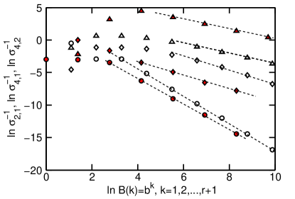
Figure 8: (Color online) The renormalization group factors σ2,1subscript𝜎21\sigma_{2,1}, σ4,1subscript𝜎41\sigma_{4,1}, and σ4,2subscript𝜎42\sigma_{4,2}, for the Cayley tree (empty triangles, circles and diamonds, respectively) and the diamond lattice (red filled triangles, circles and diamonds), in arbitrary units. The points for the bubble diagram, σ4,2subscript𝜎42\sigma_{4,2}, for the Cayley tree have been shifted down by two decades for better visibility. The linear fits are indicated by dashed lines.

V.2 Second order terms

To second order, there are more diagrams to consider. In the recursion relation for r0subscript𝑟0r_{0} (Eq. 58), we have expanded in r0subscript𝑟0r_{0}, which is small by assumption, and we will keep only terms that are at most second order in the small quantities v0subscript𝑣0v_{0} and r0subscript𝑟0r_{0}. In the context of the ϵitalic-ϵ\epsilon-expansion Wilson3 , to first order in ϵitalic-ϵ\epsilon one could ignore v02superscriptsubscript𝑣02v_{0}^{2} contributions to Eq.(58), by arguing that they would be of higher order in ϵitalic-ϵ\epsilon. But here we still have to consider such terms that are zeroth order in r0subscript𝑟0r_{0}.

The diagrams D2,2D_{2,2\prime} and D2,2′′subscript𝐷2superscript2′′D_{2,2^{\prime\prime}} have vanishing amplitudes, nearly ten orders of magnitude smaller than the other terms, and go like logB𝐵\log B, so we neglect them. For the Cayley tree, as explained below Eq.(53), it is not possible to get a nonzero contribution from D2,2′′subscript𝐷2superscript2′′D_{2,2^{\prime\prime}} except for the case where one has the constant vector for the outer legs and three identical internal lines, giving only a negligible amplitude. The only diagram which could contribute to the second term in Eq.(58) is D2,2subscript𝐷22D_{2,2} evaluated at r0=0subscript𝑟00r_{0}=0, so we get,

r=Bp2r0+12v0z2[Bϕ2,1(I1(0)r0I2(0))6v0Bϕ2,2].superscript𝑟superscript𝐵subscript𝑝2subscript𝑟012subscript𝑣0superscript𝑧2delimited-[]superscript𝐵superscriptsubscriptitalic-ϕ21superscriptsubscript𝐼10subscript𝑟0superscriptsubscript𝐼206subscript𝑣0superscript𝐵subscriptitalic-ϕ22r^{\prime}=B^{p_{2}}r_{0}+12v_{0}z^{2}[B^{-\phi_{2,1}^{\ell}}(I_{1}^{(0)}-r_{0}I_{2}^{(0)})\\ -6v_{0}B^{-\phi_{2,2}}]\;\;. (61)
Table 2: All the different terms which we consider to second order in the perturbative calculation of the renormalized Hamiltonian on the Cayley tree and the diamond lattice. The diagrams D2,1,D4,2subscript𝐷21subscript𝐷42D_{2,1},\ldots D_{4,2}, which are displayed in Fig. 7, have been evaluated at r0=0subscript𝑟00r_{0}=0 and we scale the maximum eigenvalue ΩΩ\Omega.
Scaling Bhv.  Cayley  Diamond
σ2,1Bϕ2,1similar-tosubscript𝜎21superscript𝐵subscriptitalic-ϕ21\sigma_{2,1}\sim B^{\phi_{2,1}} ϕ2,1=0.80±0.03subscriptitalic-ϕ21plus-or-minus0.800.03\phi_{2,1}=0.80\pm 0.03 ϕ2,1=0.75±0.02subscriptitalic-ϕ21plus-or-minus0.750.02\phi_{2,1}=0.75\pm 0.02
I1(0)(B)superscriptsubscript𝐼10𝐵I_{1}^{(0)}(B) logB𝐵\log B logB𝐵\log B
I2(0)(B)BϕI2similar-tosuperscriptsubscript𝐼20𝐵superscript𝐵subscriptitalic-ϕ𝐼2I_{2}^{(0)}(B)\sim B^{\phi_{I2}} ϕI2=1.09±0.04subscriptitalic-ϕ𝐼2plus-or-minus1.090.04{\phi_{I2}}={1.09\pm 0.04} ϕI2=0.92±0.03subscriptitalic-ϕ𝐼2plus-or-minus0.920.03{\phi_{I2}}={0.92\pm 0.03}
σ4,1Bϕ4,1similar-tosubscript𝜎41superscript𝐵subscriptitalic-ϕ41\sigma_{4,1}\sim B^{\phi_{4,1}} ϕ4,1=2.11±0.03subscriptitalic-ϕ41plus-or-minus2.110.03\phi_{4,1}=2.11\pm 0.03 ϕ4,1=1.97±0.04subscriptitalic-ϕ41plus-or-minus1.970.04\phi_{4,1}=1.97\pm 0.04
σ2,2Bϕ2,2similar-tosubscript𝜎22superscript𝐵subscriptitalic-ϕ22\sigma_{2,2}\sim B^{\phi_{2,2}} ϕ2,1=0.40±0.04subscriptitalic-ϕ21plus-or-minus0.400.04\phi_{2,1}=0.40\pm 0.04 ϕ2,1=0.60±0.03subscriptitalic-ϕ21plus-or-minus0.600.03\phi_{2,1}=0.60\pm 0.03
σ4,2Bϕ4,2similar-tosubscript𝜎42superscript𝐵subscriptitalic-ϕ42\sigma_{4,2}\sim B^{\phi_{4,2}} ϕ4,2=1.11±0.03subscriptitalic-ϕ42plus-or-minus1.110.03\phi_{4,2}=1.11\pm 0.03 ϕ4,2=1.11±0.04subscriptitalic-ϕ42plus-or-minus1.110.04\phi_{4,2}=1.11\pm 0.04

The only nontrivial one-loop contribution to the 4-vertex at second order comes from the bubble diagram D4,2subscript𝐷42D_{4,2}, since D4,2subscript𝐷4superscript2D_{4,2^{\prime}} turns out to have a vanishing amplitude as well. Let us define,

I2(B,i,j;r0)μ,μ=μB+1NG(μ)G(μ)×uμ(i)uμ(j)uμ(i)uμ(j).subscript𝐼2𝐵𝑖𝑗subscript𝑟0superscriptsubscript𝜇superscript𝜇subscript𝜇𝐵1𝑁𝐺𝜇𝐺superscript𝜇subscript𝑢𝜇𝑖subscript𝑢𝜇𝑗subscript𝑢superscript𝜇𝑖subscript𝑢superscript𝜇𝑗I_{2}(B,i,j;r_{0})\equiv\sum_{\mu,\mu^{\prime}=\mu_{B}+1}^{N}G(\mu)G(\mu^{\prime})\\ \times u_{\mu}(i)u_{\mu}(j)u_{\mu^{\prime}}(i)u_{\mu^{\prime}}(j)\;\;.

where the r0subscript𝑟0r_{0} dependence of the Green’s functions are implicit. The leading contribution from the bubble diagram to the ψ4superscript𝜓4\psi^{4} term is,

H4,2<superscriptsubscript𝐻42\displaystyle H_{4,2}^{<} =\displaystyle= 36v021,2,3,4μBψ^1ψ^2ψ^3ψ^436superscriptsubscript𝑣02superscriptsubscript1234subscript𝜇𝐵subscript^𝜓1subscript^𝜓2subscript^𝜓3subscript^𝜓4\displaystyle 36v_{0}^{2}\sum_{1,2,3,4}^{\mu_{B}}\hat{\psi}_{1}\hat{\psi}_{2}\hat{\psi}_{3}\hat{\psi}_{4}
×i,j=1NI2(B,i,j;0)u1(i)u2(i)u3(j)u4(j).\displaystyle\times\sum_{i,j=1}^{N}I_{2}(B,i,j;0)u_{1}(i)u_{2}(i)u_{3}(j)u_{4}(j)\;\;.

where r0subscript𝑟0r_{0} has been set to zero and we will drop it from the notation. To rescale this term we define

σ4,211,2,3,4μBi,j=1NI2(0)(B,i,j)u1(i)u2(i)u3(j)u4(j)Bϕ4,2.proportional-tosuperscriptsubscript𝜎421superscriptsubscript1234subscript𝜇𝐵superscriptsubscript𝑖𝑗1𝑁superscriptsubscript𝐼20𝐵𝑖𝑗subscript𝑢1𝑖subscript𝑢2𝑖subscript𝑢3𝑗subscript𝑢4𝑗similar-tosuperscript𝐵subscriptitalic-ϕ42\sigma_{4,2}^{-1}\propto\sum_{1,2,3,4}^{\mu_{B}}\sum_{i,j=1}^{N}I_{2}^{(0)}(B,i,j)u_{1}(i)u_{2}(i)u_{3}(j)u_{4}(j)\\ \sim B^{-\phi_{4,2}}\;\;. (62)

Putting together all the quartic terms we get the recursion relation for the interaction constant v𝑣v up to second order,

v=v0z4[Bϕ4,136v0Bϕ4,2].superscript𝑣subscript𝑣0superscript𝑧4delimited-[]superscript𝐵subscriptitalic-ϕ4136subscript𝑣0superscript𝐵subscriptitalic-ϕ42v^{\prime}=v_{0}z^{4}[B^{-\phi_{4,1}}-36v_{0}\,B^{-\phi_{4,2}}]\;\;. (63)

Recalling that z2=Bp1+p2superscript𝑧2superscript𝐵subscript𝑝1subscript𝑝2z^{2}=B^{p_{1}+p_{2}} (Eq. 23), and that in the present case, with β=0𝛽0\beta=0, p1=p2=1subscript𝑝1subscript𝑝21p_{1}=p_{2}=1,

v=v0B4ϕ4,1[136v0Bϕ4,2+ϕ4,1],superscript𝑣subscript𝑣0superscript𝐵4subscriptitalic-ϕ41delimited-[]136subscript𝑣0superscript𝐵subscriptitalic-ϕ42subscriptitalic-ϕ41v^{\prime}=v_{0}B^{4-\phi_{4,1}}[1-36v_{0}\,B^{-\phi_{4,2}+\phi_{4,1}}]\;\;, (64)

where we have again suppressed all numerical coefficients.

If one neglects the explicit eigenvector dependence of σ4,21superscriptsubscript𝜎421\sigma_{4,2}^{-1} and performs the sums over the lattice points, the bubble diagram essentially factorizes into the integrals over the external legs and the loop integral I2(0)Bsimilar-tosuperscriptsubscript𝐼20𝐵I_{2}^{(0)}\sim B, (Eq.V.2), so that σ4,21Bϕ4,1I2(0)similar-tosuperscriptsubscript𝜎421superscript𝐵subscriptitalic-ϕ41superscriptsubscript𝐼20\sigma_{4,2}^{-1}\sim B^{-\phi_{4,1}}I_{2}^{(0)}. The scaling behavior of all the various diagrams appearing in Fig. 7 are shown in Fig. 8. The values of the different exponents are given in Table 2. From Table 2 we see that indeed ϕ4,2ϕ4,11similar-to-or-equalssubscriptitalic-ϕ42subscriptitalic-ϕ411\phi_{4,2}\simeq\phi_{4,1}-1, bearing out our estimate for both the Cayley tree and the diamond lattice.

Using this estimate, finally we may write down the recursion relation

v=v0B4ϕ4,1(136v0I2(0)).superscript𝑣subscript𝑣0superscript𝐵4subscriptitalic-ϕ41136subscript𝑣0superscriptsubscript𝐼20v^{\prime}=v_{0}B^{4-\phi_{4,1}}(1-36v_{0}I_{2}^{(0)})\;\;. (65)

which yields the fixed point equation

v=1B(4ϕ4,1)36I2(0).superscript𝑣1superscript𝐵4subscriptitalic-ϕ4136superscriptsubscript𝐼20v^{\ast}=\frac{1-B^{-(4-\phi_{4,1})}}{36I_{2}^{(0)}}\;\;. (66)

Note that the scaling exponents involved in Eq. (64) are, within error bars, identical for the Cayley and diamond lattices. In both cases, large B𝐵B (the infrared regime) leads to the Gaussian fixed point once again since I2(0)Bsimilar-tosuperscriptsubscript𝐼20𝐵I_{2}^{(0)}\sim B. Iterating the recursion relation Eq. (64) leads to the same result.

Although the Cayley tree has a spectral dimension d~=2~𝑑2{\tilde{d}}=2, which is the lower critical dimension for models with Ising symmetry, it is well known that the Ising model on the Cayley tree has mean field behavior on the Bethe lattice (the limit of r𝑟r\to\infty limit of the Cayley tree) Eggarter ; CJThompson . In fact a tree structure is a lattice on which the Bethe-Peirls approximation is exact, in the same way as the RSRG newKadanoff ; Kadanoff ; Leeuwen is exact for the diamond latticeKaufmanandGriffiths ; GriffithsandKaufman . We should therefore expect that on the Cayley tree, the Guassian fixed point should be stable with respect to perturbation by a ψ4superscript𝜓4\psi^{4} term and that is indeed what we find.

The Ising model on the diamond lattice, on the other hand, which has the same spectral dimension as the Cayley tree, exhibits nonzero magnetization below Tc>0subscript𝑇𝑐0T_{c}>0 and non-classical exponents Bleher . We would have expected that the perturbation by a ψ4superscript𝜓4\psi^{4} term would lead to non-classical behavior for the diamond lattice, but a non-Gaussian fixed point eludes us. For Eq. (64) to yield a nonzero fixed point, with at most a logarithmic correction, one should have 4ϕ4,14subscriptitalic-ϕ414-\phi_{4,1} equal to a small constant, which one may use as an expansion parameter, and I2(0)superscriptsubscript𝐼20I_{2}^{(0)} to have at most a logarithmic dependence on B𝐵B. Note that on a Bravais lattice in d=2𝑑2d=2 dimensions, precisely the same scenario would have led to a null result within the usual Wilson momentum shell renormalization group as well.

V.3 Spectral dimension d~>2~𝑑2\tilde{d}\,>2

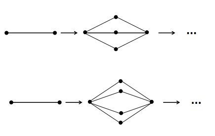
In order to see whether we can obtain a non-Gaussian fixed point for the quartic coupling constant v0subscript𝑣0v_{0} and non-trivial critical exponents for d~>2~𝑑2\tilde{d}\,>2, we have utilized a generalization of the diamond lattice Itzykson illustrated in Fig. 9, with p𝑝p parallel paths replacing a bond and each path consisting of bssubscript𝑏𝑠b_{s} steps. This yields a fractal dimension of df=ln(pbs)/lnbssubscript𝑑𝑓𝑝subscript𝑏𝑠subscript𝑏𝑠d_{f}=\ln(p\,b_{s})/\ln b_{s}. We take bs=2subscript𝑏𝑠2b_{s}=2 as in the foregoing sections, but vary p𝑝p and numerically calculate the spectral dimension d~~𝑑\tilde{d} from the scaling exponent β𝛽\beta in the region of small ω𝜔\omega. The relevant exponents ϕ4,1Ωsubscriptsuperscriptitalic-ϕΩ41\phi^{\Omega}_{4,1}, ϕ4,2Ωsubscriptsuperscriptitalic-ϕΩ42\phi^{\Omega}_{4,2}, ϕ4,2Ωsubscriptsuperscriptitalic-ϕΩ4superscript2\phi^{\Omega}_{4,2^{\prime}} and ζΩ4lnz/lnBsuperscript𝜁Ω4𝑧𝐵\zeta^{\Omega}\equiv 4\ln z/\ln B are provided in Table 3. In this section we scale the maximum eigenvalue and therefore we will again omit the superscript ΩΩ\Omega in the remainder of the section, although we keep it in the tables for clarity. In dimensions d~>2~𝑑2\tilde{d}>2, we have not attempted to factorize the contributions from the outer legs and the internal loops, as we do not have a sufficient understanding of how the vertex ΦΦ\Phi behaves.

Within our perturbative scheme up to second order in v𝑣v, Eq. (64) is in the form of a one-dimensional iterative map which can be written as v=a1v(1a2v)superscript𝑣subscript𝑎1𝑣1subscript𝑎2𝑣v^{\prime}=a_{1}v(1-a_{2}v), with a1=Bζϕ4,1subscript𝑎1superscript𝐵𝜁subscriptitalic-ϕ41a_{1}=B^{\zeta-\phi_{4,1}} and a2=36Bϕ4,1[Bϕ4,2+43Bϕ4,2]subscript𝑎236superscript𝐵subscriptitalic-ϕ41delimited-[]superscript𝐵subscriptitalic-ϕ4243superscript𝐵subscriptitalic-ϕ4superscript2a_{2}=36\,B^{\phi_{4,1}}[B^{-\phi_{4,2}}+\frac{4}{3}B^{-\phi_{4,2^{\prime}}}], where, for p>2𝑝2p>2 we include the diagram D4,2subscript𝐷4superscript2D_{4,2^{\prime}} as it has a non-vanishing amplitude and an exponent close to that of D4,2subscript𝐷4superscript2D_{4,2^{\prime}}. The iteration converges to a stable non-Gaussian fixed point v=(a11)(a1a2)1superscript𝑣subscript𝑎11superscriptsubscript𝑎1subscript𝑎21v^{\ast}=(a_{1}-1)(a_{1}a_{2})^{-1} in the interval v(0,a21)superscript𝑣0superscriptsubscript𝑎21v^{\ast}\in(0,a_{2}^{-1}) provided 1<a1<31subscript𝑎131<a_{1}<3.

We can read off from Table 3 that at p=2𝑝2p=2, the trajectory of v𝑣v is chaotic and goes off to infinity as the maximum of the vsuperscript𝑣v^{\prime} curve exceeds 1/a21subscript𝑎21/a_{2}. A non-Gaussian fixed point exists and is stable for p=3,4,5𝑝345p=3,4,5, while for p=7𝑝7p=7, d~=4.12>4~𝑑4.124\tilde{d}=4.12>4, we find a1=3.5>3subscript𝑎13.53a_{1}=3.5>3, so the non-zero fixed point looses its stability.
Refer to caption
Figure 9: The generalized hierarchical lattice a là Itzykson and Luck Itzykson , shown for p=3𝑝3p=3 and p=4𝑝4p=4 parallel paths with bs=2subscript𝑏𝑠2b_{s}=2 steps each.
Table 3: Higher spectral dimensions: Generalized diamond lattice (Fig. 9). The spectral density exponent β𝛽\beta, spectral dimension d~~𝑑\tilde{d}, the exponents for the field renormalization factor z4superscript𝑧4z^{4} and for the Feynman diagrams contributing to the quartic coupling constant, as well as the coefficient aΩsuperscript𝑎Ωa^{\Omega} and the stable fixed point vsuperscript𝑣v^{\ast} are provided for different p7𝑝7p\leq 7; for p7𝑝7p\geq 7, d~>4~𝑑4\tilde{d}>4. See text for definitions.
p𝑝p β𝛽\beta d~~𝑑\tilde{d} ζΩsuperscript𝜁Ω\zeta^{\Omega} ϕ4,1Ωsubscriptsuperscriptitalic-ϕΩ41\phi^{\Omega}_{4,1} ϕ4,2Ωsubscriptsuperscriptitalic-ϕΩ42\phi^{\Omega}_{4,2} ϕ4,2Ωsubscriptsuperscriptitalic-ϕΩ4superscript2\phi^{\Omega}_{4,2^{\prime}} a1Ωsuperscriptsubscript𝑎1Ωa_{1}^{\Omega} vsuperscript𝑣v^{\ast}
2 0 2 4 1.99 1.11 1.425 4 0
3 0.40 2.80 4.80 3.25 2.34 2.24 2.93 0.00400.00400.0040
4 0.66 3.32 5.32 4.13 3.75 3.89 2.28 0.00540.00540.0054
5 0.83 3.46 5.66 4.14 3.31 3.54 2.87 0.00480.00480.0048
7 1.06 4.12 6.12 4.31 4.43 5.75 3.5 0
Table 4: Higher spectral dimensions: the exponents for the quadratic terms, and the specific heat exponent α𝛼\alpha.
p𝑝p   ϕ2,1;0Ωsubscriptsuperscriptitalic-ϕΩ210\phi^{\Omega}_{2,1;0}   ϕ2,1;1Ωsubscriptsuperscriptitalic-ϕΩ211\phi^{\Omega}_{2,1;1}   ϕ2,2Ωsubscriptsuperscriptitalic-ϕΩ22\phi^{\Omega}_{2,2}   ϕ2,2Ωsubscriptsuperscriptitalic-ϕΩ2superscript2\phi^{\Omega}_{2,2^{\prime}}   ϕ2,2′′Ωsubscriptsuperscriptitalic-ϕΩ2superscript2′′\phi^{\Omega}_{2,2^{\prime\prime}} rsuperscript𝑟r^{\ast}\quad Ytsubscript𝑌𝑡Y_{t} α𝛼\alpha δ𝛿\delta
2 0.83±0.06plus-or-minus0.830.060.83\pm 0.06 0.14±0.04plus-or-minus0.140.040.14\pm 0.04 0.02±0.08plus-or-minus0.020.080.02\pm 0.08 0.04±0.03plus-or-minus0.040.03-0.04\pm 0.03 0.10±0.03plus-or-minus0.100.030.10\pm 0.03 0 111 0 \infty
3 1.27±0.08plus-or-minus1.270.081.27\pm 0.08 0.77±0.07plus-or-minus0.770.070.77\pm 0.07 1.06±0.08plus-or-minus1.060.081.06\pm 0.08 0.73±0.13plus-or-minus0.730.130.73\pm 0.13 0.90±0.06plus-or-minus0.900.060.90\pm 0.06 0.1130960.113096-0.113096 1 1.14 6
4 1.82±0.24plus-or-minus1.820.241.82\pm 0.24 1.49±0.22plus-or-minus1.490.221.49\pm 0.22 1.91±0.26plus-or-minus1.910.261.91\pm 0.26 1.37±0.21plus-or-minus1.370.211.37\pm 0.21 1.49±0.09plus-or-minus1.490.091.49\pm 0.09 0.061920.06192-0.06192 1 0.58 4.03
5 1.58±0.12plus-or-minus1.580.121.58\pm 0.12 1.36±0.12plus-or-minus1.360.121.36\pm 0.12 1.69±0.13plus-or-minus1.690.131.69\pm 0.13 1.31±0.11plus-or-minus1.310.111.31\pm 0.11 1.34±0.16plus-or-minus1.340.161.34\pm 0.16 0.14901970.1490197-0.1490197 1 0.75 3.41
7 1.91±0.24plus-or-minus1.910.241.91\pm 0.24 1.78±0.23plus-or-minus1.780.231.78\pm 0.23 2.03±0.25plus-or-minus2.030.252.03\pm 0.25 1.71±0.23plus-or-minus1.710.231.71\pm 0.23 1.76±0.23plus-or-minus1.760.231.76\pm 0.23 00 1 0 3

We now consider the iterative equation for r𝑟r, which is in the form r=arrcrsuperscript𝑟subscript𝑎𝑟𝑟subscript𝑐𝑟r^{\prime}=a_{r}r-c_{r}, where the coefficients depend upon vsuperscript𝑣v^{\ast}. Defining the scaling exponents ϕ2,1;0subscriptitalic-ϕ210\phi_{2,1;0} and ϕ2,1;1subscriptitalic-ϕ211\phi_{2,1;1} for the zeroth and first order terms of the expansion in r0subscript𝑟0r_{0} of σ2,11subscriptsuperscript𝜎121\sigma^{-1}_{2,1}, we have

ar=Bp212vB12ζϕ2,1;1,subscript𝑎𝑟superscript𝐵subscript𝑝212superscript𝑣superscript𝐵12𝜁subscriptitalic-ϕ211a_{r}=B^{p_{2}}-12v^{\ast}B^{\frac{1}{2}\zeta-\phi_{2,1;1}}\;\;, (67)

and

cr=12vB12ζ[Bϕ2,1;06v(Bϕ2,2+Bϕ2,2+23Bϕ2,2′′)].subscript𝑐𝑟12superscript𝑣superscript𝐵12𝜁delimited-[]superscript𝐵subscriptitalic-ϕ2106superscript𝑣superscript𝐵subscriptitalic-ϕ22superscript𝐵subscriptitalic-ϕ2superscript223superscript𝐵subscriptitalic-ϕ2superscript2′′c_{r}=12v^{\ast}B^{\frac{1}{2}\zeta}[B^{-\phi_{2,1;0}}\;\\ -6v^{\ast}(B^{-\phi_{2,2}}+B^{-\phi_{2,2^{\prime}}}+\tfrac{2}{3}B^{-\phi_{2,2^{\prime\prime}}})]\;\;. (68)

The fixed point rsuperscript𝑟r^{\ast} is unstable, with |ar|>1subscript𝑎𝑟1|a_{r}|>1 and negative since the critical temperature increases with the interactions.

The linearized transformation matrix for r𝑟r and v𝑣v is upper triangular, and r/r|v=arBYtevaluated-atsuperscript𝑟𝑟superscript𝑣subscript𝑎𝑟similar-tosuperscript𝐵subscript𝑌𝑡\partial r^{\prime}/\partial r|_{v^{\ast}}=a_{r}\sim B^{Y_{t}} by our definition. The critical exponent α𝛼\alpha can now be found from differentiating Eq. (24) twice with respect to t𝑡t and using chtαsimilar-tosubscript𝑐superscript𝑡𝛼c_{h}\sim t^{-\alpha}. One gets α=2p1/Yt𝛼2subscript𝑝1subscript𝑌𝑡\alpha=2-p_{1}/Y_{t}. We calculate Ytsubscript𝑌𝑡Y_{t} from Eq. (67) by comparing the exponents of the first and second terms in arsubscript𝑎𝑟a_{r} , and we find ζ/2ϕ2,1;1>1𝜁2subscriptitalic-ϕ2111\zeta/2-\phi_{2,1;1}>1 all cases where v0superscript𝑣0v^{\ast}\neq 0.

For p=7𝑝7p=7, with v=0superscript𝑣0v^{\ast}=0, the only surviving term in arsubscript𝑎𝑟a_{r} is the Gaussian one. Then Yt=1subscript𝑌𝑡1Y_{t}=1 and from Eq. (25) we find α=2(1+β)𝛼21𝛽\alpha=2-(1+\beta). However, for β=1.06>1𝛽1.061\beta=1.06>1, the ultraviolet singularity in

ch0Ωdωωβ(r0+ω)2similar-tosubscript𝑐superscriptsubscript0Ω𝑑𝜔superscript𝜔𝛽superscriptsubscript𝑟0𝜔2c_{h}\sim\int_{0}^{\Omega}\frac{d\omega\;\omega^{\beta}}{(r_{0}+\omega)^{2}}\;\; (69)

takes over and we find α=0𝛼0\alpha=0. The values of α𝛼\alpha for different p𝑝p are given in Table 4.

Since the field renormalization z𝑧z has not changed in this second order perturbation expansion, the eigenvalue for the external field hh, namely BYh=zsuperscript𝐵subscript𝑌𝑧B^{Y_{h}}=z is still given by Eq. (26). In terms of β𝛽\beta we have δ=(2+β)/β𝛿2𝛽𝛽\delta=(2+\beta)/\beta. The values are listed in Table 4. Clearly for β=1𝛽1\beta=1, we get δ=3𝛿3\delta=3, the mean field value. Actually one may show by the methods of Section IIIC that for β>1𝛽1\beta>1 (or d~>4~𝑑4\tilde{d}>4), where v0subscript𝑣0v_{0} is an irrelevant variable, that δ=3𝛿3\delta=3.

VI Conclusions and discussion

The eigenvalue spectrum of the graph Laplacian has already been used to define an effective dimensionality which governs both vibrational and diffusive behavior, as well as the infrared singularities of the Gaussian model Dhar ; Cassi ; Hattori on arbitrary lattices. Bradde et al. Bianconi2010 have discussed the Ginzburg criterion for phase transitions on spatial complex networks in terms of the spectral dimension d~~𝑑{\tilde{d}} of the closely related adjacency matrix. The present paper is complementary to the approach of Bradde et al. Bianconi2010 , in the sense that we study non-spatial networks, although both the Cayley tree and the diamond lattice are embeddable in two dimensions.

We build the spectral renormalization group method on the generalized Fourier transform using the eigenvectors of the graph Laplacian. We show how to implement a renormalization group a là Wilson on non-translationally invariant non-spatial networks, either by changing the upper cutoff of the eigenvalues of the graph Laplacian (in place of the momentum cutoff on Bravais lattices) or by scaling the total number of nodes (which is the same as the number of eigenvectors of the graph Laplacian). The lack of translational invariance forces us to avoid length-rescaling altogether, since the only thermodynamically meaningful length, the correlation length, is not well defined on these lattices GriffithsandKaufman . The hyperscaling relations cannot be used, since it is not quite clear how the dimension should be defined GriffithsandKaufman (embedding dimension d𝑑d, fractal dimension dfsubscript𝑑𝑓d_{f}, or spectral dimension d~~𝑑\tilde{d}). It should be noted that the exact real space renormalization group for Ising spins on the diamond lattice, applied blindly as a length rescaling, yields an eigenvalue for the reduced temperature yt=0.7479subscript𝑦𝑡0.7479y_{t}=0.7479, a correlation length exponent ν=1.3370𝜈1.3370\nu=1.3370 and, if the hyperscaling relation (with d=df=d~=2𝑑subscript𝑑𝑓~𝑑2d=d_{f}=\tilde{d}=2) is used, a rather embarrasing α=0.6738𝛼0.6738\alpha=-0.6738.

For the Gaussian model, we find that the critical exponents depend exclusively on the spectral dimension through β𝛽\beta, the scaling exponent of the spectral density in the infrared region. Note that β=d~21𝛽~𝑑21\beta=\tfrac{\tilde{d}}{2}-1. The Gaussian fixed point is stable with respect to the introduction of quartic couplings in d~=2~𝑑2\tilde{d}=2. This seems to be due to the fact that the spectral dimensionality d~~𝑑\tilde{d} is equal to the lower critical value within the Ising universality class, rather than to the lack of translational invariance Melrose or some other exotic property of the diamond lattice. It has been remarked by Wilson and Kogut Wilson3 ( p. 124), that reaching the non-trivial fixed point is difficult in two (Euclidean) dimensions, as the fixed point functions acquire a sensitive dependence on the choice of the initial function to be iterated. Several authors Bagnuls ; Morris have found that in fact, scalar field theories in two dimensions may not be amenable to perturbative RG schemes.

We have gone to higher fractal and spectral dimensions by using a generalized diamond lattice Itzykson , using an integer parameter, p𝑝p (see Fig. 9). The spectral dimension is raised from two towards four (β=1𝛽1\beta=1), we encounter stable non-Gaussian fixed points. We are able to calculate the eigenvalues for all the different diagrams in the perturbation expansion up to second order, and compute the specific heat exponent. As the spectral dimension is raised beyond four, although the fixed point still exists, it looses its stability. (In fact iterations for the coupling constant v0subscript𝑣0v_{0} exhibit a period four attractor, however this does not carry much physical meaning because it depends purely on the truncation of the perturbation expansion).

Note that, due to the strong dependence on the eigenvectors of the graph Laplacian that is introduced by the 4-vertex ΦΦ\Phi (Eq. 46), we are forced to resort to numerical computations in order to extract the eigenvalues, and beyond Gaussian theory we are not able to express them solely in terms of the spectral dimension. However, better analytical understanding of the symmetries of the eigenvectors should allow us to extract more information. Work is under progress in this direction.

We conclude that critical fluctuations on non-translationally invariant networks are amenable to investigation by the present method. Only near lower critical dimensions for the universality class under study, the perturbative scheme might break down.

One question is how to go to higher orders in perturbation theory. In this paper we have gone only up to second order in the coupling constant and/or the reduced temperature. This, however, is not enough to introduce corrections to the field renormalization z𝑧z, and the computation of the critical exponent η𝜂\eta may be problematic for the same reasons as that of ν𝜈\nu.

Acknowledgements

It is a pleasure to thank E. Brezin, B. Derrida, J.-P. Eckmann, M. Mungan, H. Özbek and T. Turgut for a number of interesting discussions. A. Tuncer acknowledges partial support from the ITUBAP No. 36259.

Appendix A.1 Square and Cubic Lattices

In Figs. A.1,A.2, we present plots for the numerical calculation of the spectral density and the exponent β𝛽\beta for the square lattice (N=4×10⁴𝑁4superscript104N=4\times 10^{4}) and the cubic lattice (N=(35)3𝑁superscript353N=(35)^{3}). In Figs. A.3, A.4, the scaling plots for the exponents ϕ1,ϕ2,p1subscriptitalic-ϕ1subscriptitalic-ϕ2subscript𝑝1\phi_{1},\;\;\phi_{2},\;\;p_{1} and p2subscript𝑝2p_{2} are displayed. A summary of all the critical exponents computed in this paper was given in Table 1 in the main text.

For many networks, even in the thermodynamic limit the spectral density does not become a smooth function which behaves as a power law, ρ(ω)ωβsimilar-to𝜌𝜔superscript𝜔𝛽\rho(\omega)\sim\omega^{\beta} for small ω𝜔\omega. In particular, the spectral density of the Barabasi-Albert network BA , as well as scale free networks with γ>3𝛾3\gamma>3 grow exponentially for small ω𝜔\omega (so that the spectral dimension diverges), although they have a power law tail for large ω𝜔\omega, Ref. erzan .) As in the case of the Cayley tree and the diamond hierarchical lattice, the spectral density may be nonzero only on a union of discrete sets of measure zero. Where one cannot compute ρ(ω)𝜌𝜔\rho(\omega) analytically, one should be aware that its numerical determination may call for prohibitively large network sizes, as has also been noted by Bradde et al. Bianconi2010 . Even for Bravais lattices with p.b.c., the convergence of the numerical spectral density to the thermodynamic limit is very slow, especially in the small ω𝜔\omega region, see Figs. A.1,A.2.

Table A.1: The eigenvalues and eigenvectors of the Cayley tree with two generations (r=2𝑟2r=2) and branching number b=3𝑏3b=3. The integers in the first line of the table below indicate the nth𝑛𝑡nth distinct eigenvalue ω(n)superscript𝜔𝑛\omega^{(n)}.The eigenvalues are, in increasing order, ω(1)=0,ω(2)=(α+1)/α+,ω(3)=1,ω(4)=b+1b,ω(5)=(α1)/α=1/ω(2),ω(6)=b+1+bformulae-sequenceformulae-sequencesuperscript𝜔10formulae-sequencesuperscript𝜔2subscript𝛼1subscript𝛼formulae-sequencesuperscript𝜔31formulae-sequencesuperscript𝜔4𝑏1𝑏superscript𝜔5subscript𝛼1subscript𝛼1superscript𝜔2superscript𝜔6𝑏1𝑏\omega^{(1)}=0,\;\omega^{(2)}=(\alpha_{+}-1)/\alpha_{+}\;,\omega^{(3)}=1,\omega^{(4)}=b+1-\sqrt{b},\;\omega^{(5)}=(\alpha_{-}-1)/\alpha_{-}=1/\omega^{(2)},\;\omega^{(6)}=b+1+\sqrt{b}, with α±=1±1+4/b2subscript𝛼plus-or-minusplus-or-minus114𝑏2\alpha_{\pm}=\frac{1\pm\sqrt{1+4/b}}{2}. Defining θ=2π/b𝜃2𝜋𝑏\theta=2\pi/b, the numerical factors appearing in the eigenvectors μ=2,3,11,12𝜇231112\mu=2,3,11,12 and 4,,9494,\ldots,9 are the real and imaginary parts of exp(iθ),=1,2,,bformulae-sequence𝑖𝜃12𝑏\exp(i\ell\theta),\;\ell=1,2,\ldots,b. The constants appearing in columns marked 4 and 6 are p=bb𝑝𝑏𝑏p=-b-\sqrt{b}, and q=b+b𝑞𝑏𝑏q=-b+\sqrt{b}. The normalization constants have not been included for clarity. Notice the wide disparity between the 222nd and 555th, and resp. 444tn and 666th eigenvalues belonging to eigenvectors with the same symmetries.
1 2 2 3 3 3 3 3 3 4 5 5 6
1 0 0 0 0 0 0 0 0 b3superscript𝑏3-\sqrt{b^{3}} 0 0 +b3superscript𝑏3+\sqrt{b^{3}}
1 -1/2 3/232\sqrt{3}/2 0 0 0 0 0 0 p -1/2 3/232\sqrt{3}/2 q𝑞q
1 -1/2 3/232-\sqrt{3}/2 0 0 0 0 0 0 p -1/2 3/232-\sqrt{3}/2 q𝑞q
1 1 0 0 0 0 0 0 0 p 1 0 q𝑞q
1 (1/2)α+12subscript𝛼-(1/2)\alpha_{+} (3/2)α+32subscript𝛼(\sqrt{3}/2)\alpha_{+} -1/2 0 0 3/232\sqrt{3}/2 0 0 1 (1/2)α12subscript𝛼-(1/2)\alpha_{-} (3/2)α32subscript𝛼(\sqrt{3}/2)\alpha_{-} 1
1 (1/2)α+12subscript𝛼-(1/2)\alpha_{+} (3/2)α+32subscript𝛼(\sqrt{3}/2)\alpha_{+} -1/2 0 0 -3/232\sqrt{3}/2 0 0 1 (1/2)α12subscript𝛼-(1/2)\alpha_{-} (3/2)α32subscript𝛼(\sqrt{3}/2)\alpha_{-} 1
1 (1/2)α+12subscript𝛼-(1/2)\alpha_{+} (3/2)α+32subscript𝛼(\sqrt{3}/2)\alpha_{+} 1 0 0 0 0 0 1 (1/2)α12subscript𝛼-(1/2)\alpha_{-} (3/2)α32subscript𝛼(\sqrt{3}/2)\alpha_{-} 1
1 (1/2)α+12subscript𝛼-(1/2)\alpha_{+} (3/2)α+32subscript𝛼-(\sqrt{3}/2)\alpha_{+} 0 -1/2 0 0 3/232\sqrt{3}/2 0 1 (1/2)α12subscript𝛼-(1/2)\alpha_{-} (3/2)α32subscript𝛼-(\sqrt{3}/2)\alpha_{-} 1
1 (1/2)α+12subscript𝛼-(1/2)\alpha_{+} (3/2)α+32subscript𝛼-(\sqrt{3}/2)\alpha_{+} 0 -1/2 0 0 -3/232\sqrt{3}/2 0 1 (1/2)α12subscript𝛼-(1/2)\alpha_{-} (3/2)α32subscript𝛼-(\sqrt{3}/2)\alpha_{-} 1
1 (1/2)α+12subscript𝛼-(1/2)\alpha_{+} (3/2)α+32subscript𝛼-(\sqrt{3}/2)\alpha_{+} 0 1 0 0 0 0 1 (1/2)α12subscript𝛼-(1/2)\alpha_{-} (3/2)α32subscript𝛼-(\sqrt{3}/2)\alpha_{-} 1
1 α+subscript𝛼\alpha_{+} 0 0 0 -1/2 0 0 3/232\sqrt{3}/2 1 αsubscript𝛼\alpha_{-} 0 1
1 α+subscript𝛼\alpha_{+} 0 0 0 -1/2 0 0 3/232-\sqrt{3}/2 1 αsubscript𝛼\alpha_{-} 0 1
1 α+subscript𝛼\alpha_{+} 0 0 0 1 0 0 0 1 αsubscript𝛼\alpha_{-} 0 1
Refer to caption
Figure A.1: The spectral density for the 200×\times 200 square lattice, ρ(ω)ωβsimilar-to𝜌𝜔superscript𝜔𝛽\rho(\omega)\sim\omega^{\beta}, with β=0.00±0.02𝛽plus-or-minus0.000.02\beta=0.00\pm 0.02 for small ω𝜔\omega. The first 13 points have been fitted.
Refer to caption
Figure A.2: The spectral density for the N=353=42875𝑁superscript35342875N=35^{3}=42875 cubic lattice with periodic boundary conditions. ρ(ω)ωβsimilar-to𝜌𝜔superscript𝜔𝛽\rho(\omega)\sim\omega^{\beta}, with β=0.50±0.03𝛽plus-or-minus0.500.03\beta=0.50\pm 0.03. Here ρ(ω)𝜌𝜔\rho(\omega) is fitted from the 2nd to the 35th point.
Refer to caption
Figure A.3: (Color online)The rescaling factors σ1Vsubscriptsuperscript𝜎V1\sigma^{\rm V}_{1} (blue, triangles), σ2Vsubscriptsuperscript𝜎V2\sigma^{\rm V}_{2} (black, squares), σ1Ωsubscriptsuperscript𝜎Ω1\sigma^{\Omega}_{1} (red, circles) and σ2Ωsubscriptsuperscript𝜎Ω2\sigma^{\Omega}_{2} (green, diamonds) for the square lattice, some symbols fall on top of each other. The exponents are ϕ1,ϕ2,p1,p2subscriptitalic-ϕ1subscriptitalic-ϕ2subscript𝑝1subscript𝑝2\phi_{1},\phi_{2},p_{1},\;p_{2} are given in the legend. The scale factors are B(k)=N/k𝐵𝑘𝑁𝑘B(k)=N/k, k=1,,N/2𝑘1𝑁2k=1,...,N/2. The scaling region is taken from k=4𝑘4k=4 to k=1000𝑘1000k=1000 .
Refer to caption
Figure A.4: (Color online) The RG factors σ1Vsubscriptsuperscript𝜎V1\sigma^{\rm V}_{1} (blue, triangles), σ2Vsubscriptsuperscript𝜎V2\sigma^{\rm V}_{2} (black, squares), σ1Ωsubscriptsuperscript𝜎Ω1\sigma^{\Omega}_{1} (red, circles) and σ2Ωsubscriptsuperscript𝜎Ω2\sigma^{\Omega}_{2} (green, diamonds) for the cubic lattice with periodic boundary conditions. All the points after the first two have been fitted. The numerical values of the exponents are provided in the legend.

Appendix A.2 Eigenvalues and eigenvectors of the graph Laplacian

Closed form expressions for the eigenvalues of the graph Laplacian of the Cayley tree are known Rojo ; Rabbiano ; however, to our knowledge, explicit solutions for all the eigenvalues for arbitrary r𝑟r are not available. (Also see Rozikov and coworkers Rozikov2006 ; Rozikov2013 ; Rozikov_Rev_2013 ). We present in Table A.1, the eigenvalues and eigenvectors of the graph Laplacian for the Cayley tree with r=2.

Ochab et al.Burda provide valuable insights into the successive stages of symmetry breaking leading to the different eigenvectors and the eigenvalues of the adjacency matrix of the Cayley tree. We have been able to analytically compute the eigenvectors for arbitrary r𝑟r, for ω<ω𝜔superscript𝜔\omega<\omega^{\ast}, using the automorphism properties of the Cayley tree; this will be presented in a separate publication. For larger trees, the same pattern (Table A.1) is stretched to the whole tree, and then, for increasing ω𝜔\omega, becomes localized on subtrees of diminishing size.
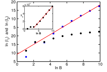
Refer to caption
Figure A.5: Scaling behavior of I1(0)superscriptsubscript𝐼10I_{1}^{(0)} (circles) and I2(0)superscriptsubscript𝐼20I_{2}^{(0)} (squares) for the Cayley tree. The data points for I1(0)superscriptsubscript𝐼10I_{1}^{(0)} are better fitted by lnB𝐵\ln B, as seen in the inset. The slope of the fitted line is 1.09±0.04plus-or-minus1.090.041.09\pm 0.04, gives I2(0)B1.09±0.04similar-tosuperscriptsubscript𝐼20superscript𝐵plus-or-minus1.090.04I_{2}^{(0)}\sim B^{1.09\pm 0.04}.

Appendix A.3 Scaling of the functions IK(0)subscript𝐼𝐾0I_{K}(0) on the Cayley tree

Here we would like to calculate explicitly the functions IK(B)subscript𝐼𝐾𝐵I_{K}(B), K=1,2𝐾12K=1,2,

IK(B)μ=μBNωμK,subscript𝐼𝐾𝐵superscriptsubscript𝜇subscript𝜇𝐵𝑁superscriptsubscript𝜔𝜇𝐾I_{K}(B)\equiv\sum_{\mu=\mu_{B}}^{N}\omega_{\mu}^{-K}\;\;, (A.1)

for the Cayley tree, making use of the approximate formulae (Eqs. 31,32). Let us take the scaling factor to equal powers of the branching number b𝑏b, so that Bk=bksubscript𝐵𝑘superscript𝑏𝑘B_{k}=b^{k}. We see that already for k=1𝑘1k=1, the eigenvalues included in the sum will be below the peak at ω=1superscript𝜔1\omega^{\ast}=1, where the equations cited above hold to a good approximation. Defining nksubscript𝑛𝑘n_{k} as the label of the smallest distinct eigenvalue compatible with μBksubscript𝜇subscript𝐵𝑘\mu_{B_{k}},

IK(0)=AK+n=nkrτn[ω(n)]K.superscriptsubscript𝐼𝐾0subscript𝐴𝐾superscriptsubscript𝑛subscript𝑛𝑘𝑟subscript𝜏𝑛superscriptdelimited-[]superscript𝜔𝑛𝐾I_{K}^{(0)}=A_{K}+\sum_{n=n_{k}}^{r}\tau_{n}[\omega^{(n)}]^{-K}\;\;. (A.2)

Note that for k=r𝑘𝑟k=r, N/Br1similar-to-or-equals𝑁subscript𝐵𝑟1N/B_{r}\simeq 1. The constant AKsubscript𝐴𝐾A_{K} is the sum of [ω(n)]Ksuperscriptdelimited-[]superscript𝜔𝑛𝐾[\omega^{(n)}]^{-K} over all n𝑛n such that ω(n)>1superscript𝜔𝑛1\omega^{(n)}>1. Then

IK(0)=AK+n=nkrb(n2)(b1)anb(rn+2)K.superscriptsubscript𝐼𝐾0subscript𝐴𝐾superscriptsubscript𝑛subscript𝑛𝑘𝑟superscript𝑏𝑛2𝑏1subscript𝑎𝑛superscript𝑏𝑟𝑛2𝐾I_{K}^{(0)}=A_{K}+\sum_{n=n_{k}}^{r}\frac{b^{(n-2)}(b-1)}{a_{n}b^{-(r-n+2)K}}\;\;. (A.3)

Approximating ansubscript𝑎𝑛a_{n} by a constant as before, canceling bnsuperscript𝑏𝑛b^{n} in the summand and using nk=rk+1subscript𝑛𝑘𝑟𝑘1n_{k}=r-k+1 and rnk1=k𝑟subscript𝑛𝑘1𝑘r-n_{k}-1=k we find for K=1𝐾1K=1,

I1(0)=A1+(b1)brak,superscriptsubscript𝐼10subscript𝐴1𝑏1superscript𝑏𝑟𝑎𝑘I_{1}^{(0)}=A_{1}+\frac{(b-1)b^{r}}{a}k\;\;, (A.4)

or

I1(0)=const.+(b1)bralnblnBk,formulae-sequencesuperscriptsubscript𝐼10const𝑏1superscript𝑏𝑟𝑎𝑏subscript𝐵𝑘I_{1}^{(0)}={\rm const.}+\frac{(b-1)b^{r}}{a\ln b}\ln B_{k}\;\;, (A.5)

where the dependence on the scaling parameter in only logarithmic. Similarly, one gets,

I2(0)=A2+br+2(bk1)a2superscriptsubscript𝐼20subscript𝐴2superscript𝑏𝑟2superscript𝑏𝑘1superscript𝑎2I_{2}^{(0)}=A_{2}+\frac{b^{r+2}(b^{k}-1)}{a^{2}} (A.6)

giving

I2(0)=const.+br+2a2Bk,formulae-sequencesuperscriptsubscript𝐼20constsuperscript𝑏𝑟2superscript𝑎2subscript𝐵𝑘I_{2}^{(0)}={\rm const.}+\frac{b^{r+2}}{a^{2}}B_{k}\;\;, (A.7)

where the dependence on the scaling parameter B𝐵B is linear. It should be noted that brNproportional-tosuperscript𝑏𝑟𝑁b^{r}\propto N in all of the above.

References

  • (1) M. Newman, A.-L. Barabàsi, D.J. Watts, The Structure and Dynamics of Networks, (Princeton University Press, 2006)
  • (2) G. Caldarelli, A. Vespignani, Large scale structure and dynamics of complex networks : from information technology to finance and natural science (World Scientific, 2007)
  • (3) A. Barrat, M. Barthélemy, A. Vespignani, Dynamical Processes on Complex Networks (Cambridge University Press, 2008)
  • (4) R. Albert and A.-L. Barabasi, Rev. Mod. Phys. 74 47 (2002).
  • (5) S.N. Dorogovtsev, A.V. Goltsev, J.F.F. Mendes, Rev. Mod. Phys. 80, 1275 (2008)
  • (6) K.G. Wilson, Phys. Rev. B 4, 3174 (1971)
  • (7) K.G. Wilson, Phys. Rev. B 4, 3184 (1971)
  • (8) K.G. Wilson, Phys. Rev. Lett. 28 548 (1972)
  • (9) K.G. Wilson and J. Kogut, Phys. Rep. 12, 75 (1974)
  • (10) S. Bradde, F. Caccioli, L. Dall’Asta, G. Bianconi, Phys. Rev. Lett. 104, 218701 (2010).
  • (11) Th. Niemeijer and J. M. J. Van Leeuwen, ”Renormalization theory for Ising-like spin systems,” in Phase transitions and critical phenomena, Vol. 6 (1976) 425-505
  • (12) T.W. Burkhardt, J.M.J. van Leeuwen, Real-Space Renormalization (Springer, 1982)
  • (13) E. Efrati, Z. Wang, A. Kolan, and L.P. Kadanoff, Rev. Mod. Phys. 86, 647 (2014).
  • (14) C. Song, S. Havlin and H.A. Makse, Nature, 433, 392 (2005).
  • (15) E. Aygün, A. Erzan, J. Phys. Conf. Ser. 319, 012007 (2011).
  • (16) Chung FRK 1997, Spectral graph theory, (Washington DC: American Mathematical Society)
  • (17) A.N. Berker and S. Ostlund, J. Phys. C 12, 4961 (1979).
  • (18) T.H. Berlin and M. Kac, Phys. Rev.86, 821 (1952).
  • (19) K. Huang, Statistical Mechanics, 2nd ed. (John Wiley and Sons, N.Y., 1987), pp. 434-436.
  • (20) N. Goldenfeld, Lectures on phase transitions and the renormalization group (Perseus Books, Reading Mass., 1992)
  • (21) D.J. Amit, Field Theory, the Renormalization Group, and Critical Phenomena, 3rd Edition (World Scientific, 2005).
  • (22) C.J. Thompson, J. Stat. Phys. 27, 441 (1982)
  • (23) O. Rojo and M. Rabbiano, Linear Algebra Appl. 427, 138 (2007).
  • (24) R.B. Griffiths and M. Kaufman, Phys. Rev. B 26 5022 (1982)
  • (25) A. Erzan, Physica A Lett. 225, 235 (1997).
  • (26) T. Eggarter, Phys. Rev. B 9, 2989 (1974)
  • (27) M. Kaufman and R.B. Griffiths, Phys. Rev. B 24 496 (1981)
  • (28) O. Rojo and R. Soto, Linear Algebra Appl. 403, 97 (2005)
  • (29) J.K. Ochab and Z. Burda, Phys. Rev. E 85, 021145 (2012)
  • (30) L.P. Kadanoff and A. Houghton, Phys. Rev. B 11, 377 (1975)
  • (31) P.M. Bleher and E.Zalys, Comm. Math. Phys. 120, 409 (1989).
  • (32) C. Itzykson and J.M.Luck, “Zeroes of the partition Function for Statistical Models on Regular and Hierarchical Latices,” in V. Ceauşescu, G. Costache, and V. Georgescu Eds., Critical Phenomena, Proceedings, Braşov School Conference ( Prog. Phys. vol. 11) (Springer 1985).
  • (33) D. Dhar, J. Math. Phys, 18 577 (1977)
  • (34) R. Burioni, and D. Cassi, Phys. Rev. Lett. 76, 1091 (1996).
  • (35) K. Hattori, T. Hattori and H. Watanabe, Prog. Theor. Phys. 92, 108 (1987).
  • (36) J.R. Melrose, J. Phys. A 16 1041 1983.
  • (37) C. Bagnuls and C. Bervillier, Phys. Rep. 348 91 (2001).
  • (38) T. Morris, Phys. Lett. B 345, 139 (1995).
  • (39) É.P. Normatov and U.A. Rozikov, Math. Notes 79, 399 (2006).
  • (40) D. Gandolfo, F.H. Haydarov, U.A. Rozikov, and J. Ruiz, J. Stat. Phys. 153, 400 (2013).
  • (41) U.A. Rozikov, Rev. Math. Phys. 25 1330001 (2013).