Computation of the Halo Mass Function Using Physical Collapse Parameters: Application to Non-Standard Cosmologies
Abstract
In this article we compare the halo mass function predicted by the excursion set theory with a drifting diffusive barrier against the results of N-body simulations for several cosmological models. This includes the standard CDM case for a large range of halo masses, models with different types of primordial non-Gaussianity, and the Ratra-Peebles quintessence model of Dark Energy. We show that in all those cosmological scenarios, the abundance of dark matter halos can be described by a drifting diffusive barrier, where the two parameters describing the barrier have physical content. In the case of the Gaussian , the statistics are precise enough to actually predict those parameters at different redshifts from the initial conditions. Furthermore, we found that the stochasticity in the barrier is non-negligible making the simple deterministic spherical collapse model a bad approximation even at very high halo masses. We also show that using the standard excursion set approach with a barrier inspired by peak patches leads to inconsistent predictions of the halo mass function.
1 Introduction
The abundance of dark matter halos is sensitive to both the initial
statistics of the matter density field
[1, 2, 3, 4] and the
gravitational collapse, which has led to their formation
(e.g. [6, 5, 7]). Hence, the abundance
of these virialized structures at different cosmic times is sensitive
to the underlying cosmology (e.g. [9, 10, 11]). Therefore an
accurate modelling of the halo mass function is crucial for future
observational analysis, but additionally it may provide a physical
understanding of halo formation. A successful framework to predict the
halo abundances is the excursion set theory [12]. Given the
initial statistics of the matter density field and collapse
criteria, one can compute the prediction of the mass
function. Nevertheless, the exact analytical predictions are not
necessarily easy to compute. The often applied approximations
lead to unrealistic mass definitions and barrier thresholds. Recently [17] described, how to implement
corrections induced by a realistic mass definition based on [12]. In addition, they
implemented consistently a barrier which is not described by a
deterministic value, but scatters around its mean value [18] -
see also [56, 57, 58, 59, 60, 61, 62, 63]
for others literature on stochastic barrier.
The same formalism had been extended in [20, 14, 21, 22] to the case
where the mean threshold depends on the variance of the density field inspired
by the ellipsoidal collapse [27], leading to a drifting diffusive
barrier (DDB).
However, the quantitative values of the barrier required to reproduce
N-body simulations with high accuracy (), are significantly
different to the ellipsoidal collapse expectations. In [23] the
authors showed that the discrepancy is due to the intrinsic
assumption of the excursion set theory, which does not take into
account that halos form at special positions in the initial matter
density field (mostly associated with peak locations, see
[53] [58, 28, 34]) leading to a larger scatter than expected.
In this paper we investigate further the robustness of the DDB model and its physical meaning by predicting the barrier parameters at different redshift from the initial conditions of the N-body simulations. We also test its ability to model the halo mass function measured from non-standard cosmological simulations and discuss the pertinence of assuming non-universal parameters for the barrier.
In section 2 of this paper we first briefly review the drifting diffusive barrier model [21, 20, 14, 22], built upon [18, 17, 19]. Then we show that the collapse overdensity measured in N-body simulations required to form halos is well approximated by this model, while a different type of barrier inspired by the physics of collapsing peaks leads to inconsistent predictions once it is plugged into the standard excursion set approach[12]. In section 2.3 we explore in detail the large mass limit of our model. In section 3 we use the values describing the barrier measured from the initial conditions to predict the halo mass function at and compare it against the results of N-body simulations. Finally, we test the ability of the model to describe the halo mass function in various non-CDM cosmologies in section 4.
2 The Excursion Set Theory Barrier Modelling
The first attempt to predict the halo mass function was done by Press Schechter [8]. The idea is to relate the number density of halos of mass to the fraction of volumes in which the overdensity smoothed on scale is greater than some critical threshold. However, the overdensity contained in those regions can cross the threshold at different smoothing scales leading to the so called cloud-in-cloud problem. This issue is resolved in the excursion set theory [12], in which the smoothing scale is decreased from infinity until the smoothed overdensity crosses the threshold for the first time. The mass which corresponds to this scale defines the mass of the halo. The smoothed overdensity is given by
| (2.1) |
where is the Fourier transform of the filter function which defines the mass enclosed in the region of radius with , where is the mean background matter density and . Therefore, as the radius decreases the overdensity performs a random walk and the properties of this random walk depend on the filter function and the initial statistics of the matter density field. Once the filter function is specified, there is a one-to-one relationship between and the associated variance of the field
| (2.2) |
where P(k) is the linear matter power spectrum. The halo mass function can be written as:
| (2.3) |
where is the so-called multiplicity function and , with F(S) the fraction of collapsed volume with mass . Let us denote the collapse threshold by and the probability density of finding an overdensity smoothed on a scale R(S), which has never crossed on any larger scale. Hence, the fraction of collapsed volume is given by
| (2.4) |
Therefore, the two building blocks which need to be specified are the criteria of collapse and the PDF associated with the random walks of , which never crossed the barrier on scales larger than . For a sharp- filter and Gaussian initial conditions, the random walk performed by is Markovian, i.e. the evolution at a given step is independent of the previous steps. In this particular case and for some specific barrier, the exact first-crossing distribution can be solved fully analytically [12]. However, the volume defined by a top hat filter in -space leads to [17]: . This volume is inconsistent with the ones used for observations and N-body simulations. There one generally assumes spherical filters with finite support. Hence, a better filter is the top hat filter in real space, which clearly has the advantage of having a non-ambiguous volume definition. In such a case all the steps in a trajectory are correlated with one another and there is no exact analytical solution. One way to overcome this problem is to run Monte Carlo random walks as described in [12] and solve numerically for the first-crossing rate. However, this is computationally expensive111See [65] for a computationally cheap algorithm which returns an approximation of the first crossing distribution.. In [17], the authors apply a path integral formalism to compute analytically the non-Markovian corrections associated with the sharp-x filter. In this framework, the problem is fully specified by the correlators of the trajectories. For Gaussian initial conditions the only correlators which are required to specify the statistical properties of the density field, are the mean and the covariance. In such a case, and , where and is the amplitude of this non-Markovian correction, which is only weakly dependent on the smoothing scale, and is set by the linear matter power spectrum. For a universe . In [14] the authors show that the first-order correction in is sufficient to recover the exact Monte Carlo solution within for the model of barrier which reproduced the N-body simulations also within . This barrier has been extended to more general shapes in [7], although in a different context. Again the agreement between theory and Monte Carlo was within . In the limit of deterministic barriers the theory could require higher order correction in [15]. However as it was shown in [23], deterministic barriers cannot be used in the excursion set theory consistently with the initial threshold measured in N-body simulations. Furthermore, accurate predictions for the mass function with respect to N-body simulations require a stochastic barrier [14].
2.1 Mapping the Critical Threshold in N-body Simulations to the Barrier Model
In the simplest version the excursion set approach assumes a deterministic spherical collapse threshold [6]. However, initial overdense patches of matter are ellipsoidal and are sensitive to both the internal and external shear fields leading to a stochastic barrier [26, 27, 28, 29]. Furthermore, in [28] the authors found that on average smaller proto-halos require a higher overdensity in order to collapse. That analysis uses the center of the proto-halos to compute the critical overdensity. In this case the mean is well approximated by (with , ), while its variance is of order [23] (see [18] for another derivation of the variance using the ellipsoidal collapse model). Assuming the evolution of the collapse threshold at a given scale is uncorrelated to the collapse at other scales, it is possible to introduce a parameter which models the amplitude of the scatter around the mean of the barrier: . See also [23] for a discussion of this model. For , the barrier is deterministic. One could think of estimating using the ellipsoidal collapse model but this would be wrong because the excursion set theory averages over trajectories without taking into account whether their positions correspond to a peak or not [63, 12, 15, 16]. Thus, the amplitude of the scatter based on the standard ellipsoidal collapse is expected to be smaller compared to the variance of the barrier at a random position inside the proto-halo. Indeed, our physical intuition is that once we sit on a peak, we are less sensitive to the external shear field. Therefore the question is: What is the barrier we need to use in the standard excursion set framework? In order to account for the excursion set averaging over all positions, [23] showed that one should consider a threshold distribution which corresponds to the overdensity around a randomly selected halo particle and not the one which corresponds to the center of mass of the proto-halo. In other words, the critical overdensity distribution, which has led to the formation of halos, can be reconstructed by measuring the density fluctuation in the initial conditions around a randomly selected particle which belongs to a proto-halo of Lagrangian size222The Lagrangian radius of a halo is defined such that the mass inside a sphere of radius in the early homogeneous universe is equal to the halo mass. . By identifying the measured critical overdensity with the overdensity at first crossing of the barrier, i.e. , one can map the measured overdensity distribution to the barrier distribution needed for the excursion set formalism.
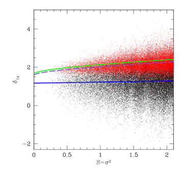
To see how the critical overdensity distribution changes when we consider a random position of the proto-halo instead of the center of mass position, we show in Fig. 1 the result of the two approaches obtained from the initial conditions of an N-body simulation. Red dots correspond to the center of mass overdensity, while black dots are for randomly selected halo particles. As expected, the scatter of the red distribution is sharper than the black distribution. In addition, the centre of mass overdensities are mostly positive, suggesting that most proto-halos correspond to initial peaks [53]. The associated PDF can be approximated by a log-normal distribution [34, 23]. The blue dashed line in Fig. 1 shows the mean prediction of the ellipsoidal collapse [27], while the solid green line shows the mean that we measure for the center of mass distribution. The blue solid line is the mean associated with the randomly selected halo particle (black distribution). A quantitative analysis is given in the Table 1 of [23]. At fixed scale , it is shown in [23] that the PDF of at random positions inside the proto-halo is very well approximated by a simple Gaussian distribution over the range of masses probed. Furthermore, after mapping the barrier distribution required to fit the N-body halo mass function to the distribution, one recovers the shape, width, and mean of the distribution measured from the random halo particles (see [23]). In contrast, in this article we start from the initial conditions of the matter density field and infer from the proto-halos the parameters of the collapse barrier. We then use these collapse parameters to predict the mass function.
In order to do this we first have to establish the link between the
PDF of the barrier and the PDF of the critical overdensity threshold
at which the random walk of crosses the barrier for the first time.
A general derivation can be found in
[23], however we propose here an alternative, more straightforward
approach, which leads to the same expression as Eq.(11) in
[23].
In the simple case where the barrier is given by a Gaussian with mean and variance , the probability to obtain B on a given scale S is
| (2.5) |
and for Gaussian initial distribution of the matter density field the probability to get an overdensity on scale is
| (2.6) |
Therefore we can introduce the ensemble of values where . If the random walk performed by is independent of (i.e. =0 [20, 14, 21, 23])333This assumption can be physically motivated, e.g. [27] presented a model in which the collapse barrier depends on the traceless shear, which is independent of . Therefore, the intersection of those two sets of values at a given is simply given by
| (2.7) |
where
| (2.8) |
Thus the PDF of the crossing height is given by
| (2.9) |
To derive the PDF of for the first time, i.e. the first-crossing distribution , we should compute the PDF associated with under the condition that on all larger scale: .
For Markovian walks (sharp- filter for and ), the above expression also describes the PDF of the first-crossing height because the walks do not keep memory of what happen at other scales.
In the general case, however, the first-crossing condition (i.e. random walk with absorbing boundary condition) might involve non-Markovian corrections when is smoothed with a sharp- filter while the barrier is not [63, 23]. These corrections play a role at low masses (large ) and are negligible at high masses where a large collapsing patch can rarely be embedded by a larger collapsing one (cloud-in-cloud problem [12]).
However in what follow we use an empirical approach: as we find in [23], neglecting this condition only affect the mean value of . The agreement between the Monte Carlo and Eq.(2.9) is quite accurate for the variance while the mean value is systematically higher for the theory compared to the Monte Carlo. In addition this shift depends on . Thus we introduce a correction term such as
| (2.10) |
and we fixe by measuring the mean value of the Monte Carlo. Using the values reported in the Tab 1 of [23], we find in average that . Therefore, in what follows we will use Eq. (2.9) with
| (2.11) |
to establish the link between the parameters of the barrier ( and ), which we use in the excursion set, and the initial critical overdensity distribution measured around randomly selected halo particles: .
2.2 Measurement of the Barrier Parameters from the Intial Conditions
In order to determine the values of the barrier we follow the procedure described in [23]. We assume that the PDF of is Gaussian given by Eq.(2.9) and we consider a Gaussian barrier with free parameters and with mean and variance . We also assume that for the mass range we probe, the linear approximation of the barrier is accurate as suggested by [23]. This assumption will be further investigated in section 2.3.
Using Eq.(2.11), the two parameters and are fitted to
the mean and variance of the initial overdensity around random proto-halo particles
measured from the initial conditions of N-body simulations.
For the analysis, we use the DEUS consortium N-body simulations [30]
(described in [31, 32, 33]). The box lengths of the simulations
are 162, 648 and 2592 Mpc, respectively, and each simulation has
particles. The simulations have been carried out using the
RAMSES code [35] for a CDM model calibrated
to the WMAP-5-year data [36] (i.e. ). The halos were identified using the
Friend-of-Friends (FoF) algorithm with linking length .
Binning the data in and using all the mass range covered by the simulation for (i.e. where the consistency is very accurate), we derive by a simple -fit the following best-fit parameters of the DDB barrier for several redshifts: () (), (), (). We tested the covariance between and by running first a fit for then and we found consistent values with the computed on a two by two grid which set simultaneously the value of and .
Note that these values are in good agreement with the ones found in the analysis of [23] that uses the mass function to determine those values and checks the consistency with the initial distribution of over a smaller sample of mass. In addition, these values may change for different initial realizations of the density field. This cosmic variance is not taken into account in this analysis.444we thank the referee for pointing this additional source of variance. Later we will use these parameters to predict the halo mass function. In Fig. 2 we show the best linear fit to the measured mean and variance. The error bars show the Poisson error. The rather large scatter (larger than the statistical error) in is probably due to systematics in the computation of the initial overdensity. Because particles are set on a grid at the beginning of the simulation, the estimation of the density of proto-halos is biased. Using Next Grid Point (NGP) charge assignment to estimate the density, we obtain huge spurious oscillations in (especially for small halos). Using Cloud In Cell (CIC) charge assignment allows us to reduce oscillations down to the level of other systematic and statistical errors.
Overall, the linear modelling of the variance and the mean describes the simulation data well. However, for small , i.e. large halos masses, it seems that the linear model with zero variance for underpredicts the variance of the barrier. Note that standard spherical collapse predicts strictly zero scatter. This will be discussed further in the next section.
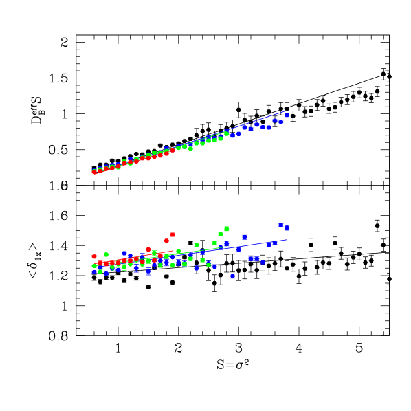
Another point we can see from this figure and the predicted DDB parameters, is a consistency between their evolution on the redshift. In average tends to increases with z while tends to decreases. Since is summed with , it is not surprising that it should increases with z because in the spherical collapse model increases at higher redshift to reach the EdS value . Perhaps more interesting is that seems to decreases with z. If a part of the stochasticity is due to late time merging halos then one could hope that at higher redshift the barrier is more deterministic ( should decreases). Nevertheless the main component of this stochasticity must be attributed to averaging over random positions when we compute the multiplicity function within the excursion set theory.
2.3 The Large Mass Limit
A common way to compute the effect of modified gravity or dark energy models on the formation of halos is to compute the spherical collapse threshold in those non-standard cosmologies (e.g. [31, 32]) and use it to predict the mass function. As we already know, the spherical collapse is based on unrealistic assumptions: no external or internal shear. However one could hope that in the large mass limit, where , these assumptions become more realistic. In such case, the mean and the variance of the barrier should converge to the spherical collapse barrier (i.e. ).
We test this assumption by analysing the PDF associated with for randomly selected halo particles and for the center of mass positions of massive halos. We measure the distributions from the initial conditions of the N-body simulation with a box length of . This large box enables us to probe even very massive halos with good statistics, for which one would expect the spherical collapse to be a good approximation. Note that this large box was not used in [23].
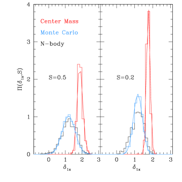
Fig. 3 shows the distribution of the critical density contrast measured in the initial conditions - leading to the formation of halos at z=0. The two panels correspond to two different mass of halos: () and (). The PDF of associated with the center of mass particles is the red histogram while for randomly selected particles it is the black histogram. In those two bins the total number of halos are for and for , . The binning is in .
The Monte Carlo prediction of this PDF is also shown by the blue histogram. It is obtained by generating numerically random walk with the barrier parameters measured for the halos from the initial conditions. We record for each walk the first-crossing values (i.e. when ) and make a histogram of those values given the two extreme masses we consider here. The prediction Eq.(2.9) is the solid blue curve. For those we use the best fit values of that we determined in [23]. This figure shows that the linear barrier modelling holds for but for very massive halos () the width of the measured distribution is significantly larger than the linear model predicts. The measured mean and variance are (1.16,0.11) at and (1.2,0.3) at . In addition we report a skewness at and at which is compatible with the one measured in the Monte Carlo.
On the other hand, the PDF associated with the center of mass seems to converge to a deterministic value. The mean and the variance are () and ().
As pointed out in [23], the variance here is larger than that measured in [64]. This difference might be due to the fact that we built this center-of-mass PDF assuming initial proto-halo to be spherical as it was done in [34].
Using these measurements of the mean and variance and those reported in [23], we find that the associate PDF can be well-fitted by the following log-normal distribution (red solid line):
| (2.12) |
where and with
. Note that the mean
value is in reasonable agreement with [27]: it is systematically
rescaled by a factor . On the other hand, the variance is in
disagreement with the theoretical ellipsoidal prediction from
[18] and [23]. As mentioned in [23], this discrepancy may be due to the
fact that our estimate of is broadened as a consequence
of having assumed spherical proto-halo which is usually not the case.
Overall, this analysis indicates that the linear model for the mean of is in reasonable agreement with the critical overdensity measured in N-body simulations. However, for very massive halos, the scatter around the mean is larger than expected and not consistent with the model. Hence, the predicted halo mass function might not be able to reproduce the N-body simulation in this limit. This was not observed in [23], where the mass function as well as the distribution was well modelled by the linear DDB model. Note, however, that the largest halo mass studied in [23] was much smaller, (), than in our current study. We will test the accuracy of the mass function predictions in Section 3.
One could think about solving the first-crossing distribution for a barrier which mimics the center of mass distribution of (Eq. (2.12)). In the next section we will see that such a barrier will lead to inconsistent results for the halo mass function. This confirms the idea that the standard excursion set framework requires a barrier modelling valid for random positions and not for special positions like density peaks.
2.4 The Barrier for Peaks
We can perform one further test on the modelling of the barrier, which
enters the excursion set theory. Previously we assumed a Gaussian
barrier and showed that the N-body first-crossing
distribution is well reproduced by the analytical theory once we use the barrier measured from random halo particles. One might wonder
if one can also use a barrier inspired by peak statistics, which when
used in the standard excursion set framework, is able to recover the PDF of
associated with the center-of-mass of the proto-halo
(the red distribution in Fig.1 described by Eq.(2.12)). In fact, we
previously saw that had a slightly
different mean and a very different variance than expected from
the ellipsoidal collapse theory ([27, 18]). However, if we also
use a log-normal distribution for the barrier, we might expect
that the mean and the variance of the first-crossing distribution get
shifted compared to the ones we set for (See also [63]).
Thus we might ask: what is
the PDF of the barrier which at first crossing leads to Eq.(2.12)? And
subsequently, is a log-normal barrier able to predict the halo mass
function measured from N-body simulations?
To answer the first question, we ran Monte Carlo walks using a PDF for the barrier calibrated on the center-of-mass PDF Eq.(2.12) (with ). In fact it is easy to extend the generation of random walks for barriers which have a log-normal distribution instead of a normal one. If is a random variable which has a normal distribution with mean and variance , then will have a log-normal distribution with a mean value and variance . Inverting these relations, we generated Monte Carlo walks using a log-normal distribution for the barrier.
It is easy to check the resulting Monte Carlo distribution is in good agreement with the theoretical formula of a log-normal distribution.
We found that at first crossing the PDF of is also a log-normal with a mean shifted to lower values,
which can be fitted by a factor . Thus in order to reproduce
the PDF of that we measured from the initial
conditions of the N-body simulations, we should use a log-normal
barrier in the excursion set as given by Eq.(2.12) with
parameters . However,
the associated mass function is completely offset to the mass function
measured from N-body simulations. This is not surprising since the
excursion set is unable to distinguish whether the trajectories belong
to the center of the peak or not. The PDF of first-crossing returned
by the excursion set theory is the one of for a randomly
selected particle. Therefore any barrier which predicts only positive
values of (such as the log-normal) cannot lead to a
consistent distribution of , especially at low masses
where, as shown in Fig. 1, a non-negligible part of
is negative.
Nevertheless, one could argue that the consistency is not important
as long as we can use a PDF of the barrier predicted by theory which
can reproduce the mass function. Currently, however, there is no
theory able to do so. For instance, the ellipsoidal collapse
prediction of the barrier cannot reproduce the halo mass function
once it is used in the standard excursion set approach as
we investigate here or in the excursion set peak formalism as
studied by [16]. In fact in [16] the authors had to calibrate their
barrier model based on the analysis of [34]. Thus the
main advantage of this drifting diffusive barrier is that the only
two parameters which described the barrier can be measured in the
initial conditions and lead to a very good agreement with respect to
the mass function as we show in the next section.
3 The Halo Mass Function
3.1 The Drifting Diffusive Barrier Halo Mass Function
For the DDB model barrier that we reviewed in the previous section, the corresponding multiplicity function for a generic initial statistics described by the second and third-order correlation functions is given by [14, 21, 22]
| (3.1) |
with
| (3.2) |
| (3.3) |
| (3.4) |
| (3.5) |
where and for a vanilla CDM universe555the value of is set by the linear matter power spectrum so its value does not change much for realistic cosmological scenarios and the primordial non-Gaussian term is
| (3.6) |
3.2 Comparison with N-body Simulation Using the Physical Barrier Parameters
In this section we test the DDB prediction for the mass function in the Gaussian CDM case using the parameter and that we measured from the initial conditions (see Section 2.2). This is performed by using the publicly available halo catalogues of the simulations we obtained from the DEUS collaboration, where halos had been identified using the FoF algorithm with a linking length of . Results are shown in Fig. 4, dots depict the N-body simulation data and the solid lines show the corresponding theoretical predictions Eq.(3.1) using the collapse parameters we measured in the initial conditions (see section 2). Different color show the different redshift.
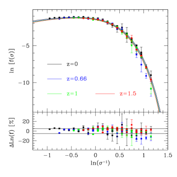
The agreement with respect to the N-body simulation is at level, which is impressive since our model for the barrier is rather simple and we use a simple mapping with Eq. (2.11) to predict the parameters for collapse. In fact, the agreement is less accurate at low mass compared to [23] where the mapping is expected to be less accurate.
3.3 Redshift evolution and non-universality of the collapse barrier
Cosmic structures carry a fossil record of the past cosmic evolution [31]. The multiplicity function therefore depends on the properties and nature of dark energy which governs the expansion rate [32]. Within the CDM cosmology, it has been shown that the multiplicity function increases () at low redshift because the dark energy density increases. At high redshift it converges to Einstein-de-Sitter values since . By looking very carefully at Fig. 4, we confirm this trend. The multiplicity at z=0 is slightly above the one at higher redshift and the multiplicity function at z=0.6, 1 and 1.5 seems too converge: this was already shown in great details in [32]. In Fig. 2, we show the mean and variance of the proto-halo overdensity in the initial density field. We could clearly see the decrease of the mean and the increase of the variance of at low redshift (black dots). This is consistent with the trend of the mass function since decreasing (and ) as well as increasing tend to increase the mass function (see for instance, [14]). At higher redshift, we also find the same order (z=0.6 then z=1, finally z=1.5) as well as a convergence towards self-similar values. By using these parameters and (which depend on redshift) within the excursion set framework, we self-consistently recover the measured multiplicity function and its variation with redshift (Fig. 4). It means that we are able for the first time to rewrite the problem of the non-universality of the mass function, as a problem of non-universality of the collapse barrier. It opens a new way to deal with the non-universality of the mass function. The original approach followed by [32, 40] is to adjust the halo-finder detection threshold as a function of so that the multiplicity function is always the same. The approach suggested by this paper would be to predict or tabulate the variation of the barrier parameters as a function of the dark energy model. Fig.2 already shows that the deviations of and are correlated to in CDM. Our goal here was to further demonstrate the self-consistency of Excursion Set Theory when varying the amount of dark energy: we can predict the halo mass function using a barrier which is set in the initial conditions of the N-body simulations. Currently, there is no successful theory able to predict this barrier from first principles. Note, however, that also for the critical overdensity around the center-of-mass of the proto-halo, the standard ellipsoidal collapse [27] is unable to accurately predict the variance of the distribution (see Table 1 in [23]) as we mentioned already in section 2.4.
4 Extension to Non-Standard Cosmology
In this section we study if the DDB model is also able to describe the halo mass function in non-standard cosmologies. First, we consider a model with different dynamics than CDM, namely a model with dynamical dark energy. Then, we alter the initial conditions and look at models with primordial non-Gaussianity.
4.1 Quintessence Model of Dark Energy

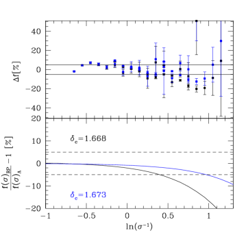
We test the robustness of the DDB model against a change in the dynamics of the universe. In particular, we consider a Ratra-Peebles (RPCDM) model of quintessence [37], which is a cosmological model with a different background expansion to the standard CDM case [32, 31, 33] and cosmological parameters in a flat universe. The N-body simulation data of this model is available on [30]. In this model the dark energy has a potential given by [37]
| (4.1) |
where is the quintessence field and , are
respectively the slope and the amplitude of the scalar
self-interaction. The N-body simulation of [31, 30] for
used . The dark energy state parameters are and the linear
matter density fluctuations such that at the normalization is
. Those choice of parameters are motivated by the analysis of WMAP5 and the UNION SN [36, 38] such that this model is not ruled out by those observations. Note that the realization of the initial Gaussian random field is identical to the CDM simulations we presented above.
First, we set the barrier for to , which corresponds to the spherical collapse value for this particular cosmological model [32]. Note, however, that the halo catalogue obtained from the simulation consists of FoF halos with a linking length of 0.2 times the mean particle separation. While for a CDM cosmology the FoF halo mass roughly corresponds to the virial halo mass at [40], this is not the case for the RPCDM model. In this cosmological model, the virial halo mass is actually smaller than the FoF halo mass. Hence, the obtained and might be biased and we do not expect that they would match with the collapse parameters measured from the initial conditions. In fact it could be that requiring a different halo finder than would for instance remove low masses halos. In this case the halos used to reconstruct the barrier would not probe the high S values of the initial distribution of the barrier.
When analysing observational data, however, one does not know the true cosmological model a priori and usually would use CDM as the fiducial cosmological model. We therefore want to test if the DDB model can still describe the halo mass function of RPCDM when assuming the wrong value for .
In principle one could infer the correct value of by reconstructing the PDF Eq.(2.9) in the limit . However we would be limited by the range cover in the simulation. Nevertheless one could test if the other parameters differ from the CDM ones. Therefore we have measured the mean and the variance of Eq.(2.9) in the initial condition and in Fig. 5 we show the ratio with respect the ones measured in the CDM simulation. First of all note that for the spherical collapse criteria, this ratio is of order which would be almost impossible to extract from the numerical uncertainty. However as we can see in Fig (5), the variance of the PDF tends to be lower than the CDM while the mean values does not differ significantly. Thus to predict the mass function of the RPCDM model, we first set the value of and using Eq.(2.11) we predict . Then we use instead to see if this would change the inferred value of . However using Eq.(2.11), we find the inferred values of does not changed. Note that the range of mass covered by the RP model is smaller than the simulation. This could affect the determination of the parameters since the distribution is less constrained at low masses ().
In the upper panel of Fig.(6), we can see the relative difference for the multiplicity function using the RPCDM N-body simulation (upper panel). The black dots show the prediction using the set of parameters () while the blue dots correspond to (). The change in results in a small difference which affect only the high mass tail of the mass function. Overall this plot shows that both predictions are in good agreements with the simulations even if it seems the second set of parameters are in better agreement. On the lower panel, we show the relative difference between the theory of the RPCDM mass function with respect to the CDM one. For the later we use the same parameters we measured in the previous section () while for the RPCDM we use the two sets of parameters ( and (). As we can see, the difference between the two becomes large if one use the predicted RPCDM value (black line).
It has been shown in [32] that the deviation to universality is higher if the algorithm finder used to detect halos is adjusted according to the virial density criteria of the considered cosmology. Similarly one could expect the same for the linear spherical threshold since there is a one-to-one mapping between the two. Hence, it would be interesting to test the sensitivity of the linear barrier using different halos finder criteria. We leave it for a future work.
Finally, this analysis shows that once again the DDB model can describe the mass function with high accuracy using only two parameters while fitting functions of the halo mass function calibrated with N-body simulations depend on several parameters. Indeed, in [14], the authors showed that the DDB model can reproduce the simulation fits over the entire redshift range used in the analysis of [42] and for different redshift. In addition, the number of parameters usually increases further when the initial conditions are not Gaussian (e.g. [41]). In the next section we will consider different types of primordial non-Gaussianities and test if the DDB model is still able to reproduce the N-body simulations data without introducing new parameters.
4.2 Primordial Non-Gaussianity
Primordial non-Gaussianity (PNG) is generated in many inflationary models (see [52] for a review), and hence measuring the type and amount of PNG provides a unique window into the physics of inflation. At leading order, non-Gaussianity can be described by the bispectrum, which is the Fourier transform of the 3-point correlation function. The amplitude of the primordial bispectrum is parametrized by and its dependence on the triangle configuration (formed by the three wave numbers , , and ) is called shape dependence. Current constraints from observations of the cosmic microwave background (CMB) [43] and the large-scale structure of the universe [44] on the level of PNG for different shapes are all consistent with zero, i.e. no significant deviations from primordial Gaussianity has been observed.
As the halo mass function is sensitive to the initial conditions, it is also a probe of PNG [45]. Compared to the CMB, which probes mostly large scales, the halo mass function measures the PNG on smaller scales (roughly on the scale of the Lagrangian radius of the halo, e.g. a few Mpc). In contrast to the scale-dependent halo bias induced by PNG [46, 47], the halo mass function is sensitive to basically all shapes of PNG [48, 49] and not only to shapes which diverge in the squeezed limit (e.g. the local type). This makes the halo mass function a complimentary probe of PNG.
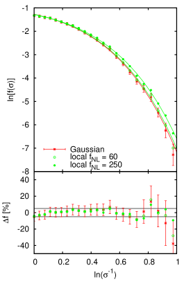
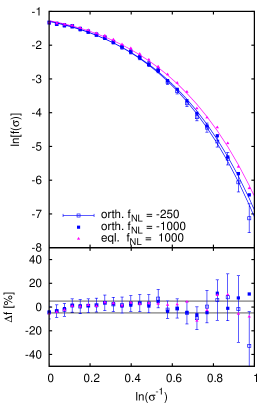
In this section, we show that the DDB model using Eq. (3.1) and
Eq. (3.6) is able to model the halo mass function of different
types of PNG with high accuracy and without introducing a new fudge factor. The only parameters which we allow to vary are the two collapse parameters and , which we fit to the mass
function derived from N-body simulations. Using the simulations of
[50], we use the halo finder of Knollmann & Knebe [51] to generate SOD halo catalogues
with halo masses defined by the mass inside a sphere with
mean overdensity of 200 times the mean background matter density.
The simulations were run with Gadget-2 and assumed a flat CDM cosmology with , , , and . The box size is 1875 and particles were used to sample the matter distribution. Further details of the simulations and the generation of the non-Gaussian initial conditions as well as a description of the different simulated types of PNG can be found in [50]. Here, we consider three different shapes of PNG: local with and , equilateral with , and orthogonal with and . Although such large values of are already ruled out by current observational constraints [43], they are still useful for model testing. The three different types of PNG differ strongly in the shape of their bispectrum: The bispectrum of the local type diverges for squeezed triangles whereas the bispectrum of the equilateral type peaks for equilateral triangles. The bispectrum shape of the orthogonal type is mathematically orthogonal to the equilateral and local shape. However, for the effect of PNG on the mass function (see Eq. 3.6), the most relevant quantity is the skewness , which is given by an integral over the bispectrum. Hence, the mass function is not very sensitive to the specific shape of the bispectrum but rather to the overall level of PNG.
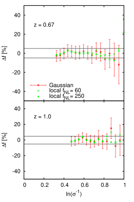
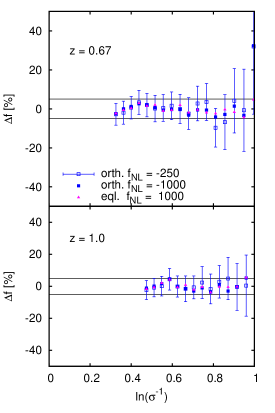
In Fig. 7, we show the measured multiplicity functions together with the best-fit DDB model predictions at . From the lower panels, which show the residuals in percent, it becomes apparent that the DDB model is capable of describing the simulation results within accuracy.
[caption=Best-fit values of the barrier parameters for different PNG models and at different redshifts. Note that due to the small mass range probed by the simulations and are strongly correlated (their correlation coefficient is )., label=table]cccc \FLPNG & redshift \MLGaussian 0 \NNGaussian 0.67 \NNGaussian 1 \MLlocal 0 \NNlocal 0.67 \NNlocal 1 \MLlocal 0 \NNlocal 0.67 \NNlocal 1 \MLorth. 0 \NNorth. 0.67 \NNorth. 1 \MLorth. 0 \NNorth. 0.67 \NNorth. 1 \MLeql. 0 \NNeql. 0.67 \NNeql. 1 \LL
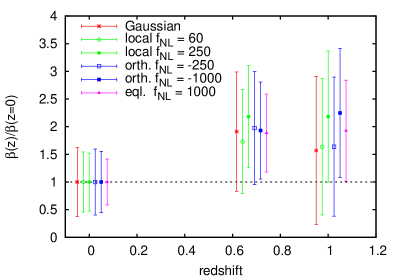
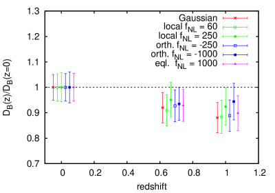
We summarize the best-fit values of and for all models at three different redshifts (0, 0.67, and 1) in Table LABEL:table. These best-fit values are sensitive to the range of mass covered by the N-body mass function and its error bars. As in the Gaussian case, the best-fit values of and vary with redshift, as shown explicitly in Fig. 8, and halo mass definition [14] (not shown here). Within the errors, the evolution with redshift of and appears independent of the nature of the initial conditions as can be seen in Fig. 8.
Hence, the simulation data suggest a single redshift evolution for all models. Note that the simulation data at different redshifts is based on the same realization of the initial density field, therefore cosmic variance, which would be present in observational data, is cancelled to a large extent in Fig. 8. This is a concern for comparisons to observations. However, when trying to understand the physical effect, we need to consider explicitly the same realisation.
Interestingly, the best-fit values also vary with the type and the level of PNG. One reason for this could be the modified distribution of eigenvalues of the initial shear field as found in the presence of primordial non-Gaussianity by [55]. The dependence of and on was already found in [21] for the local type on non-Gaussianity. There, a linear scaling in modelled the best-fit values of and well. In the analysis presented here this is the case as well. Note, however, that due to the small mass range covered by our simulations (minimum halo mass is with 100 particles), the uncertainties in the derived parameters are large and strongly correlated.
5 Conclusion
In summary, the DDB model is able to fit with high accuracy the halo mass function from N-body simulations in various (non)-standard cosmological models with only two parameters. The non-standard models we consider here are a Ratra-Peebles quintessence dark energy and various amount and shape of PNG. In the context of the DDB model, the two parameters, and , can be physically interpreted and linked to the PDF of the initial critical overdensity around randomly selected particles which will end up in halos. We also find a consistency in their evolution at different redshift showing that we are able for the first time to rewrite the problem of the non-universality of the mass function, as a problem of non-universality of the collapse barrier. A prediction of these parameters from theory is still lacking just like an accurate prediction of the PDF for critical overdensity at the center of mass of the proto-halo is currently inconsistent with the ellipsoidal collapse model [27] (e.g.[34, 23]). However, one can compute those parameters from the the proto-halo distributions as we have shown in the case of the CDM simulations, for which we had good enough statistics to do so. We found that, in general, the measured mean and variance of the critical density for collapse can be described reasonably well by a linear dependence on . For large masses, however, the scatter in the critical density for collapse measured from the initial conditions is larger than predicted by the best-fit linear model. It seems that even in the limit of , the scatter does not go to zero as expected from the spherical collapse. Nevertheless, the mass function predicted by the best-fit linear DDB model reproduces with high accuracy () the measured mass function from N-body simulations in the entire mass range. Note, that the exact values of the barrier parameters depend on the specifics of the halo finder, the redshift, the cosmological model, and the shape and amplitude of the primordial non-Gaussianity. It might also depend on the environment of the halos as it is suggested by [54]. This could lead to further investigations: How does the environment change the abundance of halos? We hope to address this question in the near future.
Acknowledgement
We are grateful to Ben Hoyle for proofreading this manuscript. This work is supported by the Trans-Regional Collaborative Research Center TRR 33 “The Dark Universe” of the Deutsche Forschungsgemeinschaft (DFG).
References
- [1] F. Lucchin and S. Matarrese, The effect of non-Gaussian statistics on the mass multiplicity of cosmic structures, Astrophys. J. 330 (1988) 535.
- [2] S. Colafrancesco, F. Lucchin and S. Matarrese, The mass function from local density maxima - Groups and clusters of galaxies, Astrophys. J. 345 (1989) 3.
- [3] W.A. Chiu, J.P. Ostriker and M.A. Strauss, Using Cluster Abundances and Peculiar Velocities to Test the Gaussianity of the Cosmological Density Field, Astrophys. J. 494 (1998) 479.
- [4] Robinson, James; Gawiser, Eric; Silk, Joseph, Constraining Primordial Non-Gaussianity with the Abundance of High-Redshift Clusters, The Astrophysical Journal, Volume 532, Issue 1, pp. 1-16.
- [5] Wang, Limin; Steinhardt, Paul J., Cluster Abundance Constraints for Cosmological Models with a Time-varying, Spatially Inhomogeneous Energy Component with Negative Pressure, The Astrophysical Journal, Volume 508, Issue 2, pp. 483-490
- [6] Gunn, James E.; Gott, J. Richard, III, On the Infall of Matter Into Clusters of Galaxies and Some Effects on Their Evolution, Astrophysical Journal, vol. 176, p.1
- [7] Kopp, Michael; Appleby, Stephen A.; Achitouv, Ixandra; Weller, Jochen, Spherical collapse and halo mass function in f(R) theories Physical Review D, vol. 88, Issue 8, id. 084015
- [8] Press, William H.; Schechter, Paul, Formation of Galaxies and Clusters of Galaxies by Self-Similar Gravitational Condensation, Astrophysical Journal, Vol. 187, pp. 425-438 (1974)
- [9] Vikhlinin, A.; Kravtsov, A. V.; Burenin, R. A.; Ebeling, H.; Forman, W. R.; Hornstrup, A.; Jones, C.; Murray, S. S.; Nagai, D.; Quintana, H.; Voevodkin, A., Chandra Cluster Cosmology Project III: Cosmological Parameter Constraints, The Astrophysical Journal, Volume 692, Issue 2, pp. 1060-1074 (2009).
- [10] Pillepich, Annalisa; Porciani, Cristiano; Reiprich, Thomas H. The X-ray cluster survey with eRosita: forecasts for cosmology, cluster physics and primordial non-Gaussianity Monthly Notices of the Royal Astronomical Society, Volume 422, Issue 1, pp. 44-69.
- [11] Mana, Annalisa; Giannantonio, Tommaso; Weller, Jochen; Hoyle, Ben; Huetsi, Gert; Sartoris, Barbara, Combining clustering and abundances of galaxy clusters to test cosmology and primordial non-Gaussianity, arXiv:1303.0287
- [12] Bond, J. R.; Cole, S.; Efstathiou, G.; Kaiser, N., Excursion set mass functions for hierarchical Gaussian fluctuations, Astrophysical Journal, Part 1 (ISSN 0004-637X), vol. 379, Oct. 1, 1991, p. 440-460.
- [13] Lacey, Cedric; Cole, Shaun, Merger rates in hierarchical models of galaxy formation, Monthly Notices of the Royal Astronomical Society (ISSN 0035-8711), vol. 262, no. 3, p. 627-649
- [14] Corasaniti, P. S.; Achitouv, I., Excursion set halo mass function and bias in a stochastic barrier model of ellipsoidal collapse, Physical Review D, vol. 84, Issue 2, id. 023009
- [15] Musso, Marcello; Sheth, Ravi K., One step beyond: the excursion set approach with correlated steps, Monthly Notices of the Royal Astronomical Society: Letters, Volume 423, Issue 1, pp. L102-L106.
- [16] Paranjape, Aseem; Sheth, Ravi K.; Desjacques, Vincent, Excursion set peaks: a self-consistent model of dark halo abundances and clustering, Monthly Notices of the Royal Astronomical Society, Volume 431, Issue 2, p.1503-1512
- [17] Maggiore, Michele; Riotto, Antonio, The Halo Mass Function from Excursion Set Theory. I. Gaussian Fluctuations with Non-Markovian Dependence on the Smoothing Scale, The Astrophysical Journal, Volume 711, Issue 2, pp. 907-927 (2010)
- [18] Maggiore, Michele; Riotto, Antonio, The Halo mass function from Excursion Set Theory. II. The Diffusing Barrier, The Astrophysical Journal, Volume 717, Issue 1, pp. 515-525 (2010).
- [19] Maggiore, Michele; Riotto, Antonio, The Halo Mass Function from Excursion Set Theory. III. Non-Gaussian Fluctuations, The Astrophysical Journal, Volume 717, Issue 1, pp. 526-541 (2010)
- [20] Corasaniti, P. S.; Achitouv, I., Toward a Universal Formulation of the Halo Mass Function, Physical Review Letters, vol. 106, Issue 24, id. 241302
- [21] Achitouv, Ixandra E.; Corasaniti, Pier Stefano, Non-Gaussian halo mass function and non-spherical halo collapse: theory vs. simulations, Journal of Cosmology and Astroparticle Physics, Issue 02, id. 002 (2012)
- [22] Achitouv, Ixandra E.; Corasaniti, Pier Stefano, Primordial bispectrum and trispectrum contributions to the non-Gaussian excursion set halo mass function with diffusive drifting barrier, Physical Review D, vol. 86, Issue 8, id. 083011
- [23] Achitouv, I.; Rasera, Y.; Sheth, R. K.; Corasaniti, P. S., Self-consistency of the Excursion Set Approach, PRL accepted (arXiv:1212.1166)
- [24] Farahi, Arya; Benson, Andrew J. Excursion set theory for correlated random walks, Monthly Notices of the Royal Astronomical Society, Advance Access. 12 pp
- [25] Lim, Seunghwan; Lee, Jounghun An extended Zel’dovich model for the halo mass function, Journal of Cosmology and Astroparticle Physics, Issue 01, article id. 019, pp. (2013).
- [26] Audit, E.; Teyssier, R.; Alimi, J.-M., Non-linear dynamics and mass function of cosmic structures. I. Analytical results., Astronomy and Astrophysics, v.325, p.439-449
- [27] Sheth, Ravi K.; Tormen, Giuseppe, An excursion set model of hierarchical clustering: ellipsoidal collapse and the moving barrier, Monthly Notices of the Royal Astronomical Society, Volume 329, Issue 1, pp. 61-75
- [28] Sheth, Ravi K.; Mo, H. J.; Tormen, Giuseppe, Ellipsoidal collapse and an improved model for the number and spatial distribution of dark matter haloes, Monthly Notices of the Royal Astronomical Society, Volume 323, Issue 1, pp. 1-12.
- [29] Desjacques, Vincent, Environmental dependence in the ellipsoidal collapse model, Monthly Notices of the Royal Astronomical Society, Volume 388, Issue 2, pp. 638-658
- [30] http://www.deus-consortium.org/
- [31] Alimi, J.-M.; Füzfa, A.; Boucher, V.; Rasera, Y.; Courtin, J.; Corasaniti, P.-S., Imprints of dark energy on cosmic structure formation - I. Realistic quintessence models and the non-linear matter power spectrum, Monthly Notices of the Royal Astronomical Society, Volume 401, Issue 2, pp. 775-790.
- [32] Courtin, J.; Rasera, Y.; Alimi, J.-M.; Corasaniti, P.-S.; Boucher, V.; Füzfa, A., Imprints of dark energy on cosmic structure formation - II. Non-universality of the halo mass function, Monthly Notices of the Royal Astronomical Society, Volume 410, Issue 3, pp. 1911-1931
- [33] Rasera, Y.; Alimi, J.-M.; Courtin, J.; Roy, F.; Corasaniti, P.-S.; Füzfa, A.; Boucher, V., Introducing the Dark Energy Universe Simulation Series (DEUSS), INVISIBLE UNIVERSE: Proceedings of the Conference. AIP Conference Proceedings, Volume 1241, pp. 1134-1139 (2010)
- [34] Robertson, Brant E.; Kravtsov, Andrey V.; Tinker, Jeremy; Zentner, Andrew R., Collapse Barriers and Halo Abundance: Testing the Excursion Set Ansatz, The Astrophysical Journal, Volume 696, Issue 1, pp. 636-652 (2009).
- [35] Teyssier, R., Cosmological hydrodynamics with adaptive mesh refinement. A new high resolution code called RAMSES Astronomy and Astrophysics, v.385, p.337-364 (2002)
- [36] Komatsu E. et al., Five-Year Wilkinson Microwave Anisotropy Probe Observations: Cosmological Interpretation, The Astrophysical Journal Supplement, Volume 180, Issue 2, pp. 330-376 (2009).
- [37] Peebles, P. J.; Ratra, Bharat, The cosmological constant and dark energy, Reviews of Modern Physics, vol. 75, Issue 2, pp. 559-606
- [38] Amanullah et al., Spectra and Hubble Space Telescope Light Curves of Six Type Ia Supernovae at 0.511 ¡ z ¡ 1.12 and the Union2 Compilation, The Astrophysical Journal, Volume 716, Issue 1, pp. 712-738 (2010)
- [39] Lewis, Antony; Bridle, Sarah, Cosmological parameters from CMB and other data: A Monte Carlo approach, Physical Review D, vol. 66, Issue 10, id. 103511
- [40] More, Surhud; Kravtsov, Andrey V.; Dalal, Neal; Gottlöber, Stefan, The Overdensity and Masses of the Friends-of-friends Halos and Universality of Halo Mass Function, The Astrophysical Journal Supplement, Volume 195, Issue 1, article id. 4, 17 pp. (2011)
- [41] Pillepich, Annalisa; Porciani, Cristiano; Hahn, Oliver, Halo mass function and scale-dependent bias from N-body simulations with non-Gaussian initial conditions, Monthly Notices of the Royal Astronomical Society, Volume 402, Issue 1, pp. 191-206
- [42] Tinker, Jeremy; Kravtsov, Andrey V.; Klypin, Anatoly; Abazajian, Kevork; Warren, Michael; Yepes, Gustavo; Gottlöber, Stefan; Holz, Daniel E., The Astrophysical Journal, Volume 688, Issue 2, pp. 709-728
- Planck Collaboration et al. [2013] Planck Collaboration, Ade, P. A. R., Aghanim, N., et al. 2013, arXiv:1303.5084
- Giannantonio et al. [2013] Giannantonio, T., Ross, A. J., Percival, W. J., et al. 2013, arXiv:1303.1349
- Matarrese et al. [2000] Matarrese, S., Verde, L., & Jimenez, R. 2000, apj, 541, 10
- Dalal et al. [2008] Dalal, N., Doré, O., Huterer, D., & Shirokov, A. 2008, prd, 77, 123514
- Matarrese & Verde [2008] Matarrese, S., & Verde, L. 2008, apjl, 677, L77
- Lo Verde et al. [2008] Lo Verde, M., Miller, A., Shandera, S., & Verde, L. 2008, jcap, 4, 14
- Wagner et al. [2010] Wagner, C., Verde, L., & Boubekeur, L. 2010, jcap, 10, 22
- Wagner & Verde [2012] Wagner, C., & Verde, L. 2012, jcap, 3, 2
- Knollmann & Knebe [2009] Knollmann, S. R., & Knebe, A. 2009, apjs, 182, 608
- [52] Bartolo, N.; Matarrese, S.; Riotto, A., Non-Gaussianity and the Cosmic Microwave Background Anisotropies, Advances in Astronomy, vol. 2010, id. 157079
- [53] Ludlow, Aaron D.; Porciani, Cristiano, The peaks formalism and the formation of cold dark matter haloes, Monthly Notices of the Royal Astronomical Society, Volume 413, Issue 3, pp. 1961-1972
- [54] Lee, Jounghun The Relative Abundance of Isolated Clusters as a Probe of Dark Energy, The Astrophysical Journal, Volume 752, Issue 1, article id. 40, 7 pp. (2012)
- Lam et al. [2009] Lam, T. Y., Sheth, R. K., & Desjacques, V. 2009, Monthly Notices of the Royal Astronomical Society, 399, 1482
- [56] A. G. Doroshkevich, Astrophyzika 3, 175 (1970).
- [57] P. Monaco, Astrophys. J. 447, 23 (1995).
- [58] J. R. Bond and S. T. Myers, Astrophys. J. Supp. 103, 1(1996)
- [59] E. Audit, R. Teyssier and J.-M. Alimi, Astron. Astrophys.325, 439 (1997).
- [60] J. Lee S. Shandarin, Astrophys. J. 500, 14 (1998).
- [61] T. Chiueh, J. Lee, Astrophys. J. 555, 83 (2001).
- [62] V. Desjacques, Mont. Not. Roy. Astron. Soc. 388, 638 (2008)
- [63] E. Castorina R. K. Sheth, Mont. Not. Roy. Astron. Soc., in press (2013).
- [64] G. Despali, G. Tormen, R. K. Sheth, Mont. Not. Roy. Astron., 431, 1143 (2013).
- [65] Musso, Marcello; Sheth, Ravi K., Monthly Notices of the Royal Astronomical Society, Volume 438, Issue 3, p.2683-2693