Kinetic theory of nonlinear diffusion in a weakly disordered nonlinear Schrödinger chain in the regime of homogeneous chaos
Abstract
We study the discrete nonlinear Schröinger equation with weak disorder, focusing on the regime when the nonlinearity is, on the one hand, weak enough for the eigenmodes of the linear problem to remain well resolved, but on the other, strong enough for the dynamics of the eigenmode amplitudes to be chaotic for almost all modes. We show that in this regime and in the limit of high temperature, the macroscopic density satisfies the nonlinear diffusion equation with a density-dependent diffusion coefficient, . An explicit expression for is obtained in terms of the eigenfunctions and eigenvalues of the linear problem, which is then evaluated numerically. The role of the second conserved quantity (energy) in the transport is also quantitatively discussed.
pacs:
05.45.-a,63.20.Pw,63.20.Ry,72.15.RnI Introduction
Disordered classical nonlinear chains are convenient model systems where the interplay between Anderson localization and classical nonlinearity can be studied. Indeed, Anderson localization is especially pronounced in one spatial dimension, where even an arbitrarily weak disorder localizes all normal modes of the linear system Gertsenshtein1959 ; Mott1961 . A nonlinearity couples the normal modes, which may lead to chaotic dynamics Zaslavsky ; Lichtenberg and destroy Anderson localization Shepelyansky1993 ; Molina1998 ; Kopidakis2008 ; Pikovsky2008 , although periodic solutions may be preserved with some probability Frohlich1986 ; Johansson2010 . Viewed from the nonlinear dynamics side, disordered nonlinear chains represent a class of dynamical systems with an infinite number of degrees of freedom, in which chaos may have a local structure in the real space Oganesyan2009 ; Basko2011 ; Pikovsky2011 ; Mulansky2011a ; Basko2012 ; Skokos2013 , and this structure can be controlled by the disorder strength.
Here we study the discrete nonlinear Schrödinger equation with disorder (DNLSE) [see Eq. (2) below]. It describes several physical systems, such as light propagating in nonlinear photonic lattices Lahini2008 or cold bosonic atoms in optical lattices in the mean-field approximation Lucioni2012 . One of the fundamental problems concerning DNLSE, as well as disordered nonlinear chains in general, is the evolution of an initially localized wave packet at very long times (see Ref. Fishman2012 for a review). In a linear system with Anderson localization, the wave packet remains exponentially localized at all times, due to the superposition principle. In the presence of a nonlinearity, the wave packet width was found to increase as a subdiffusive power of time in the direct numerical simulations of DNLSE Shepelyansky1993 ; Molina1998 ; Kopidakis2008 ; Pikovsky2008 ; Flach2009 ; Skokos2010 ; Laptyeva2010 ; Bodyfelt2011 : the second moment of the wave packet was growing as with (for the usual diffusive spreading, ). Specifically, two regimes of such subdiffusive spreading have been identified numerically: at longest observed times and at low densities, , but an intermediate range of densities and times has also been found with . These regimes were called weak and strong chaos, respectively Laptyeva2010 ; Bodyfelt2011 .
At the same time, rigorous mathematical arguments suggest that at long times the spreading, if any, should be slower than any power of Benettin1988 ; Wang2009 . Analysis of perturbation theory in the nonlinearity suggests that there is a front propagating as beyond which the wave packet is localized exponentially Fishman2009 . These arguments can be reconciled with those of the direct numerical simulations, if one assumes that the numerically observed behavior is still an intermediate asymptotics, which should break down at very long times. An indication for slowing down of the power-law subdiffusion has been observed in the scaling analysis of numerical results Mulansky2011 ; MulanskyNJP and related to the scaling of the probability of chaos with the density Mulansky2013 . A possible mechanism for breakdown of subdiffusion at long times has been suggested Michaely2012 . However, the progress in this direction is impeded by the absence of a quantitative theory for the observed power-law subdiffusion, which would (i) elucidate the main mechanism responsible for such subdiffusion, and (ii) predict quantitatively when this mechanism ceases to work.
The purpose of the present work is to construct such a theory for the intermediate spreading regime where , called “strong chaos” in Refs. Laptyeva2010 ; Bodyfelt2011 . However, the arguments of the present work are very much analogous to those used in the derivation of the kinetic equation in the theory of weak wave turbulence Zakharov . Thus, to avoid the terms “strong” and “weak”, which may be confusing, we use the term “homogeneous chaos” to denote the studied regime. The main element of the physical picture of transport developed here, is the large localization length of normal modes of the linear problem, which occurs for weak enough disorder. In this case, the nonlinearity couples each normal mode to many other modes, and if it is not too weak, the dynamics of almost all modes is chaotic. So, the chaos can be considered homogeneous both in the real space and in the mode space. The same physical image was proposed in Refs. Laptyeva2010 ; Bodyfelt2011 to identify the spreading regime with .
It has already been argued on phenomenological grounds that macroscopic transport of the conserved density in DNLSE and other disordered nonlinear chains can be described by a nonlinear diffusion equation,
| (1) |
with a -dependent diffusion coefficient Flach2010 ; Mulansky2010 . Indeed, for a power-law with some (as found in Ref. Flach2011 ), Eq. (1) gives . An expression interpolating between at higher densities and at lower densities has been proposed Laptyeva2013 , giving a crossover from to at longer times. But, again, a recent matematical work suggests that at lowest densities, should vanish faster than any power of Huveneers2013 . An explicit expression satisfying this condition has been given for the DNLSE in the limit of strong disorder and very low density, based on the picture of chaos which very inhomogeneous in space Basko2011 . Detailed quantitative understanding of the mechanisms leading to Eq. (1) with a power-law is still lacking.
In the present paper, starting from the DNLSE with weak disorder, the nonlinear diffusion equation, Eq. (1) with , is derived. An explicit expression [Eq. (60)] for is given in terms of a certain average of eigenfunctions and eigenvalues of the linear part of the DNLSE, which is then evaluated numerically. The resulting value of is in reasonable agreement with that extracted from the direct numerical simulation of Ref. Laptyeva2010 . The conditions of validity of the present approach are thoroughly discussed, and the corresponding interval of densities is identified (Fig. 5). Its lower boundary agrees with the value at which the crossover between and behavior is observed in Ref. Laptyeva2010 .
A specific property of the DNLSE is the presence of two conserved quantities: the total norm (action) and the total energy. Its consequence for the thermodynamics of the system is the existence of the so-called non-thermal states which can be described in the microcanonical ensemble, but not in the grand canonical one Rasmussen2000 . The consequence for the transport is that Eq. (1) for the norm density is not complete; the complete macroscopic description should involve two coupled equations for the norm and energy. Such coupled transport has received relatively little attention so far: a numerical study for the DNLSE without disorder is available Iubini2012 , and in the limit of strong disorder, low density, and high temperature, the off-diagonal transport coefficients were estimated to be small Basko2011 . Here, the full matrix of the transport coefficients is calculated for weak disorder, intermediate density, and high temperature. The analysis of the full coupled equations shows that in the considered regime the effect of energy transport on the norm transport is small, so Eq. (1) for only is consistent.
The paper is organized as follows. After introducing the model in Sec. II, we derive a Fokker-Planck-type master equation describing the diffusive dynamics of the normal mode actions in Sec. III. Conditions for its validity and its relation to chaos are discussed in Sec. IV. Derivation of the macroscopic Eq. (1) from the microscopic master equation, via a Boltzmann-type kinetic equation for average actions, is done in Sec. V. In Sec. VI, the role of the second conserved quantity (energy) is discussed, and the coupled macroscopic equations are analyzed. Finally, in Sec. VII, the formal expressions for the transport coefficients from Secs. V, VI are evaluated for different disorder strength, and compared to the numerics of Ref. Laptyeva2010 .
II Model and assumptions
The DNLSE reads as
| (2) |
Here labels sites of a one-dimensional lattice (the limit will be eventually taken). To each site a pair of complex conjugate variables is associated. The on-site frequencies are assumed to be random, uncorrelated, and to have the flat box distribution whose width characterizes the disorder strength. and measure the intersite coupling and the strength of the nonlinearity. The sign of is not important, as Eq. (2) is invariant under the change , , (for the latter it is important that the distribution of is symmetric).
Eq. (2) together with its complex conjugate represent the Hamilton equations for the classical Hamiltonian
| (3) |
if is treated as the canonical momentum conjugate to the coordinate . One could measure time, frequency, action, and energy in the units of , , , and , respectively, thus setting , in Eq. (2), without loss of generality. However, formal expressions are sometimes more transparent physically when written in the dimensional form, so we assume and to have the dimensionality of frequency and , respectively.
The linear part of the Hamiltonian can be diagonalized by an orthogonal transformation
| (4) |
where is the th eigenfunction of the linear problem,
| (5) |
corresponding to the eigenvalue , and is the complex amplitude of the th normal mode. The normal mode amplitudes satisfy the following equations of motion:
| (6) |
Here we introduced the overlap,
| (7) |
which is real and symmetric with respect to any permutations of the mode indices. It is a random quantity, and its statistics will play a crucial role in determining the macroscopic transport properties of the system and their dependence on the disorder strength.
The normal mode frequencies lie in the interval . Their distribution in this interval is determined by the average spectral density per unit length, . All normal mode wave functions are localized, the localization length depending on the mode frequency. The behavior of and for weak disorder is discussed in detail in Appendix A.1. Here we only note that the localization length is the largest for modes close to the center of the band, , is of the same order in the most of the band, and becomes small near the band edges. The frequency spacing between the modes which are on the same localization segment, is the smallest at .
For the transport mechanism discussed in the present work, it is crucial that , defined in Eq. (7), couples many modes. This is only possible when their localization lengths are much larger than the lattice spacing, otherwise is exponentially suppressed. The representative estimate for the localization length is , since the few tightly localized modes near the band edges contribute little to the transport. Thus, the main assumption of the present work which determines the applicability of the whole approach, is , corresponding to . Note that omitting the numerical factor from this condition would result in an unnecessarily severe restriction; in fact, the wave packet spreading with was observed in Ref. Laptyeva2010 for . At the same time, it turns out that for several quantities determined by the statistics of wave functions, the asymptotic behavior corresponding to weakest disorder is reached at really small corresponding to (see Sec. IV.3, Appendix A.2, and Ref. Kravtsov2011 )
The change of variables (4) is useful only if the dynamics of the normal mode amplitudes, , due to the last term in the right-hand side of Eq. (6), is not too fast. The relevant time scale at which the dynamics of the system allows to resolve the individual modes, is determined by the frequency spacing on one localization segment. The representative value is , so the dynamics of should be slow on the time scale . Since the nonlinear dynamics is faster for larger amplitudes, this condition imposes an upper limit on the typical norm density, , where the value of depends on the disorder strength, and is discussed in Sec. IV.3.
On the other hand, the approach developed below works if the mode dynamics is sufficiently chaotic. For this, the nonlinearity should be strong enough, so the density should not be too low, . This condition is discussed in Sec. IV.1. It will be seen that the two restrictions and are not in conflict with each other when the condition is satisfied.
Finally, the temperature is assumed to be sufficiently high, . This implies that there is no correlation between the actions and the frequencies in the initial condition for Eq. (2). It is this situation that was studied in the numerical works Shepelyansky1993 ; Molina1998 ; Kopidakis2008 ; Pikovsky2008 ; Flach2009 ; Skokos2010 ; Laptyeva2010 ; Bodyfelt2011 . In the opposite case (low ), one should minimize Hamiltonian (3) first, and then study the dynamics of the low-energy excitations. The ground state of this classical Hamiltonian at fixed extensive total norm is the Bose condensate, which is spatially non-uniform due to the disorder. The normal modes of Eq. (2), linearized around such non-uniform condensate (the Bogolyubov modes), are strongly different from the solutions of the eigenvalue problem (5) Bilas2006 ; Gurarie2008 . The assupmtion of high temperature enables one to disregard the condensate and focus on the normal modes of the linear problem (5).
III Microscopic master equation
III.1 Nonlinear frequency shifts
In the absence of the nonlinear coupling, the solution for the normal mode amplitudes is
| (8) |
where and are the action and the initial phase of the mode , respectively. With the nonlinearity included, among the terms contributing to the sum on the right-hand side of Eq. (6), there are terms oscillating at the frequency (those for which either , or , ). These, the so-called secular terms are responsible for the nonlinear shift of the th frequency:
| (9) |
This can be seen by splitting the full Hamiltonian, corresponding to Eq. (6),
| (10) |
into
| (11) |
which is integrable, and all the remaining terms, which represent an integrability-breaking perturbation. The solution of the equations of motion for the Hamiltonian is given by the same Eq. (8), but with the modified frequencies, Eq. (9), which are nothing but . Since the sum over in Eq. (9) effectively contains a large number of terms, of the order of , can be effectively replaced by its average, . Then, using the orthogonality of the eigenmode wave functions , we obtain
| (12) |
The precision of this approximation can be quantified by calculating the average relative fluctuation of the nonlinear frequency shift,
| (13) |
where averaging of the quantities that depend on is performed over the disorder realizations, and of those which depend on is over the thermal distribution (see Sec. III.4 below for details). In particular, for this distribution, , which gives Eq. (13).
Since the typical number of terms contributing to the sum over is (at larger distances decays exponentially), it is natural to expect the relative fluctuation . The same result is obtained by considering the exact expression
| (14) |
estimating , and assuming each summation to give a factor . The numerical test of this argument is performed in Appendix A.2.
III.2 Diffusion in actions
The non-secular terms in the sum on the right-hand side of Eq. (6) (i. e., those, contained in ) lead to exchange of energy between the normal modes, so that the actions change with time. Effectively, only those contribute to the sum, which correspond to the modes separated from the mode by a distance (for other modes, the overlap is exponentially small). Among those, there are terms for which all four indices are different, and terms for which at least two indices coincide. For , these latter terms can be ignored, as their role is analogous to those with are different, while their number is parametrically smaller.
Let us now consider just one term with different indices, that is, four oscillators described by the Hamiltonian
| (15) |
In principle, there are two other terms coupling the same four oscillators, and (with their complex conjugates), but we do not consider them for the moment. We have also neglected the nonlinear frequency shifts for simplicity. The first-order (in ) correction to the unperturbed solution (8) for , is given by
| (16) |
The solutions for the other three oscillators are obtained by appropriate permutations. The change in the actions of the oscillators, , is given by
| (17a) | |||
| (17b) | |||
The increment can be positive or negative, depending on the phases .
Let us now consider coupling of the mode to all other modes. The increment will be a sum of many terms with random signs, so the dynamics of the action is diffusive. To quantify this dynamics, let us calculate the phase-averaged :
| (18) |
where the prefactor prevents from double counting which originates from the symmetry , and the prime at the sum indicates that the secular terms should be excluded. The key feature of Eq. (18) is that , which is indeed a signature of the diffusive dynamics.
The -function in Eq. (18) deserves some discussion. Formally, the presented derivation is fully analogous to the derivation of the Fermi Golden Rule for decay into a continuous spectrum, familiar from quantum mechanics LL3 . However, the sum in Eq. (18) is discrete, so the function cannot be understood in the strict sense. For any finite , each individual term in the sum in the first line of Eq. (18) represents a growth for , and saturation (with oscillations) at , so it never grows linearly in time. However, when considering the whole sum, only the terms with contribute to the growth of . The number of such terms decreases , where is the typical width of the peak in , and is the typical spacing between the values of effectively contributing to the sum for various . Thus, Eq. (18) only makes sense for not too long times, , when the number of terms contributng to the sum in the first line is large. This large number of terms which enter with random phases also justifies the phase averaging in Eq. (18). This condition of large number of terms is crucial for the validity of the whole approach, and will be analyzed in detail in Sec. IV.1.
III.3 Master equation
To describe the diffusion of actions, we introduce the joint distribution function, , which depends on actions of all the normal modes. Eq. (18) together with the constraint
| (19) |
holding for each coupling term [cf. Eq. (17b)], yield a diffusion equation of the following form:
| (20) |
where the prefactor is introduced to prevent from double counting which originates from the symmetry , , (indeed, out of permutations of four different indices , only three produce distinct diffusion operators).
In Eq. (LABEL:master=) we have also included the nonlinear frequency shifts in the -function: each frequency depends on all actions , as given by Eq. (9). In fact, all reasoning of Sec. III.2 applies also to the case of shifted frequencies. Indeed, since the perturbative expressions of Sec. III.2 are valid only as long as anyway, in the derivation of Eq. (18) the frequencies can be considered fixed and determined by the instantaneous values of the actions.
III.4 Equilibrium and relaxation
The master equation (LABEL:master=) conserves the total action (norm) and total (unperturbed) energy,
| (21a) | |||
| (21b) | |||
the latter being ensured by the frequency -function with the frequencies given by Eq. (9) (the consequences of the finite width of the function are discussed in Sec. VI.2, for the moment we proceed formally). Here we introduced the averaging over the distribution function in the standard way:
| (22) |
Any distribution function depending on the actions through the combinations , will be a stationary solution of the master equation. In particular, this is the case for the thermal distribution function
| (23) |
where is the temperature and is the chemical potential. This distribution is the one that maximizes the entropy , [for which the -theorem can be straightforwardly obtained from Eq. (LABEL:master=)], under the constraint of fixed average action and energy (provided that the energy does not exceed a certain critical value Rasmussen2000 , see the discussion in Sec. VI.4).
We will be interested in the high-temperature limit
| (24) |
Then the average action or, equivalently, the average density are simply given by . (in the first case, the average is performed over the distribution function, while in the second one the average over the phases is also implied)
Let us assume that all modes are in equilibrium, except one, say, . This corresponds to the distribution function of the form
| (25) |
where is the equilibrium density, and we have taken the limit (24). Then, satisfies the following equation:
| (26) |
where we denoted
| (27) |
Eq. (26) coincides with the Fokker-Planck equation for a damped oscillator subject to external noise (see Appendix B), and has been studied in detail in Sec. 8.3 of Ref. Basko2011 . In particular, is the typical relaxation time for the mode .
III.5 Numerical evaluation of the relaxation rate
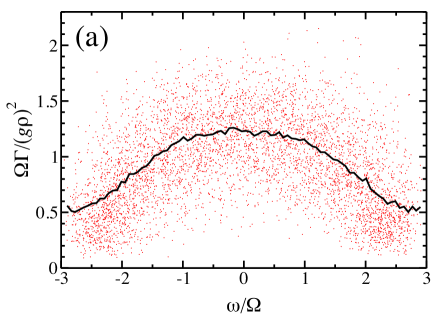
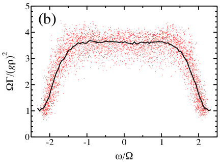
The frequency -function appearing in Eqs. (27) and (28) is implemented as a box of a finite width ,
| (29) |
where is the unit step function. This implementation is more efficient for numerical calculations than a smooth function. Using this definition, one can evaluate for each mode using Eq. (28). Two examples of such calculation are shown in Fig. 1.
Rather than looking at mode-specific quantities, we will be interested in some average characteristics. As the properties of an eigenmode are determined by its frequency, it is convenient to work with frequency-resolved averages; so we define
| (30) |
where is a sufficiently small interval, and averaging over a long chain is assumed to be equivalent to averaging over the disorder realizations. It is important that the limit should be taken prior to .
It should be emphasized that the result of the calculation of individual depends on the width . Namely, the same calculation with a larger produces an analogous picture, but the points in Fig. 1 are more squeezed towards the solid line, that is, becomes more self-averaging. For smaller , the points become more scattered. At the same time, the average is not sensitive to the value of as long as . However, at sufficiently small the values of are so scattered that the fluctuations become comparable to the average, and the latter is no longer representative. This dependence on is crucial for the discussion in Sec. IV.1 below.
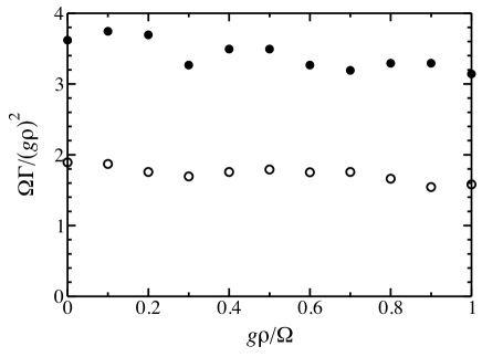
We also check numerically the dependence by evaluating Eq. (27) [again, implementing the function as in Eq. (29) and averaging over the modes at a given frequency as in Eq. (30)], where the actions are taken from the equilibrium distribution, . As seen from Fig. 2 for two values of the disorder strength, , the average is practically independent of up to the values of as large as .
IV Conditions for validity of the approach
IV.1 Low densities
The arguments of Sec. III.2 are based on the perturbative expression (LABEL:Deltac1=), which is valid only as long as the change in the actions is small compared to actions themselves, . This means that the time should be smaller than the typical action relaxation time, , introduced in Sec. III.4. If at times the discreteness of the sum in Eq. (18) is not relevant, the arguments of Sec. III.2 are self-consistent. In other words, if we take the effective width of the function to be of the order of itself, the sum in Eq. (18) should be contributed by many terms. Note that in this sense the sum in Eq. (18) and that in Eq. (28) are fully analogous. In terms of , the typical spacing between the values of effectively contributing to the sum for various , the condition of consistency is thus simply , which should hold for most of the modes .
The value of is determined both by the frequencies and by the overlaps [but not by the actions , as long as the nonlinear shifts are self-averaging, Eq. (12)]. In particular, only modes which are effectively within the same localization segment as the mode can give a significant contribution to the sum, since at large distances the overlap is exponentially suppressed. Thus, if there were no correlation between the frequencies and the overlaps , we could estimate , where is the typical spacing between different combinations of three frequencies, (see Appendix A.1 for details), for modes which are within the same localizaton length.
However, the correlation between the frequencies and the overlaps turns out to be quite strong (see Appendix A.3 for details), so it is not obvious how to actually define . This difficulty can be bypassed by noting that when the sum in Eq. (28) is contributed by many terms, should be effectively self-averaging and its fluctuations should be small, and vice versa. This is directly related to the dependence of the fluctuations of (the vertical spread of the points in Fig. 1) on the effective -function width , discussed in Sec. III.5 above. Thus, the criterion , proposed above, can be replaced by an equivalent one: the fluctuations of , evaluated for modes with frequencies at , should be small compared to the average itself. Basically, it is the same criterion that was used in Ref. BAA2006 for the validity of the kinetic equation on the metallic side of the quantum many-body localization transition.
Specifically, we focus on , assuming it to be representative of the whole band. Indeed, the results shown in Fig. 1 suggest that the dependence on is weak as long as is away from the band edges (see, hovewer, the discussion in Sec. IV.3). We then define the first and the second moments as
| (31a) | |||
| (31b) | |||
As mentioned in Sec. III.5 above, when the limit is taken, does not depend on at , so we can denote , and . The fluctuations still depend on , and we denote by the value of at which the fluctuations are equal to the average:
| (32) |
The dimensionless quantities and depend only on the dimensionless disorder strength . We can now define the minimal density as the one for which . Thus, the low-density limit of the validity of the master equation (LABEL:master=) is
| (33) |
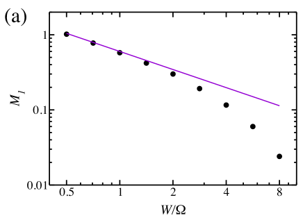
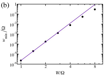
We have determined and numerically for several values of the dimensionless disorder strength in the interval , corresponding to . The value of was checked to be sufficiently small, and the chain length was checked to be sufficiently long to not affect the results (the value of could be reliably determined only for , due to computational limitations). The results are shown in Fig. 3. On the weak-disorder side, they can be fitted by
| (34a) | |||
| (34b) | |||
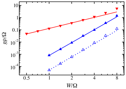
The resulting dependence of on is shown in Fig. 5 and can be fitted by
| (35) |
IV.2 Relation to chaos
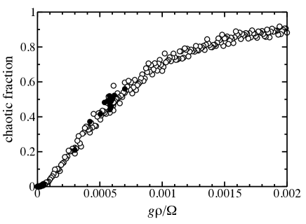
Along with , defined above by Eq. (33), we also plot the value , defined as the density at which half of the modes of the chain are chaotic and half are not. Even though only the motion of the whole coupled chain can be, strictly speaking, characterized as chaotic or not (in the sense of positive Lyapunov exponent), for given initial conditions one can focus on the dynamics of a single mode assuming the actions and phases of all other modes to be frozen, so that they represent an external (quasi-periodic) force acting on the chosen mode. For the problem of a single nonlinear oscillator under the action of an external force, one can clearly define chaotic and regular motion. Then, for the whole chain with given initial conditions, one can calculate the fraction of modes whose motion is chaotic in the above sense (see Appendix C for the details of numerical implementation). This fraction depends on the density: it vanishes when (since for a linear system no modes are chaotic) as Basko2011 ; Pikovsky2011 ; Basko2012 , and approaches unity for sufficiently large density, as shown in Fig. 4 for .
Let be the value of when the fraction is . In Fig. 5, we plot the dimensionless quantity versus disorder strength. The extracted dependence,
| (36) |
has the same power law as that for , and differs only in the prefactor. This strongly suggests that the two seemingly unrelated criteria (namely, , responsible for the self-consistency of the Fermi Golden Rule where chaos simply did not enter the discussion at all, and , ensuring that most modes are chaotic) are, in fact, closely connected. Thus, the situation analyzed in the present work corresponds to the regime when most of the modes are chaotic. This condition was used in Ref. Laptyeva2010 to define the regime of strong chaos, where the -dependence of the diffusion coefficient was observed.
IV.3 High densities
The condition for the validity of the master equation (LABEL:master=) from the high-density side is that the localized normal modes of the linear problem should be well defined on the relaxation time scale , i. e., this time should be longer than the inverse spacing between mode frequencies on the same localization segment, . In the opposite case, the discrete localized normal modes are not well resolved, and do not represent a good starting basis. Using , we can write the condition as
| (37) |
The dependence of on the disorder strength, obtained from the numerical results for and , is shown in Fig. 5. It can be fitted by the expression
| (38) |
It is instructive to approach the same condition from the clean side, treating the disorder as a perturbation. Without disorder, the normal mode wave functions and frequencies are given by
| (39) |
and for it is convenient to introduce the wave vector and velocity . It is well known that perturbative treatment of the disorder gives the elastic backscattering rate . In other words, the backscattering mean free path is twice shorter than the localization length at the same frequency Thouless1979 . At the same time, the wave functions (39) of the clean chain can be used to evaluate the mode relaxation rate due to the nonlinearity from Eq. (28), whose derivation did not assume any specific form of the wave functions. If , the elastic scattering on the disorder and Anderson localization are not important. Noting that the mean mode spacing on the localization length , we conclude that the conditions mentioned above, and are equivalent, provided that the relaxation rates (28), evaluated on clean and localized wave functions, match.
Eq. (28) with the wave functions (39) gives
| (40) |
where is a small uncertainty in the wave vector, needed to cut off the divergence at . For consistency, it should be taken of the order of the inverse mean free path, . Then, for most of the band one can write with logarithmic precision
| (41) |
However, at , expression (40) is divergent. This divergence should be smeared on the scale , so one can estimate (up to a numerical coefficient)
| (42) |
These results are confirmed by the direct numerical evaluation of Eq. (28) for different values of disorder including the disorder-free case, as shown in Fig. 6. For the disorder-free case the cutoff scale in the numerical calculation is effectively provided by the function width, , as seen by comparing curves (d) and (e) which differ by the value of used in the calculation.
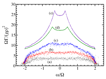
Thus, upon increasing the disorder at fixed , when (up to numerical and logarithmic factors), the localization condition becomes fulfilled for most of the normal modes, except for those in a relatively narrow frequency range ; this range shrinks completely at a stronger disorder such that . These two conditions correspond to and , respectively, which should be contrasted to following from Eq. (38). This strongly suggests that Eqs. (34a), (34b), (36), (38) [as well as Eq. (88) below] do not represent the scaling at lowest disorder strengths, but rather intermediate asymptotics. The results shown in Fig. 6 suggest that the behaviour of relaxation rates in the disordered system starts to resemble that of the clean one at , corresponding to extremely large localization lengths . The detailed investigation of this issue requires significant computational effort and is beyond the scope of the present work. We only note that similarly large localization lengths were found to be necessary to reach the weak-deisorder asymptotics in the statistics of a single normal mode wave function Kravtsov2011 .
V Macroscopic diffusion equation
The main task of the present section is to pass from the master equation (LABEL:master=), which is still microscopic as it includes the dynamics of each individual normal mode, to the macroscopic description in terms of the density. In this section, we neglect the nonlinear frequency shifts in Eq. (9). As discussed in Secs. III.1 and III.5, they produce just small corrections, , to the main result.
V.1 Classical Boltzmann equation
Multiplying Eq. (LABEL:master=) by and integrating over all actions, we obtain an equation for the average:
| (43a) | |||
| (43b) | |||
Next, we note that the action of each mode is changed due to random resonant interactions with many other modes, so any two modes effectively see mostly different resonances. Thus, one can neglect the correlations between different actions and decouple , etc. This can be done when the number of terms contributing to the sum over modes is large (see Appendix D). The latter condition was discussed in detail in Sec. IV.1.
As a result, we obtain a closed kinetic equation for the averages (the new notation is introduced for compactness):
| (44) |
This kinetic equation conserves the total action and the total energy (due to the frequency function in ). The equilibrium state, which nullifies the collision integral in the right-hand side, is given by the Rayleigh-Jeans distribution,
| (45) |
or simply in the limit (24). Eq. (45) correctly reproduces the thermodynamics of the chain with the required precision, as discussed in Appendix E.
It is worth noting that Eq. (45) represents the classical limit of the Bose-Einstein distribution , and Eq. (44) has the same form as the quantum Boltzmann equation for bosonic occupation numbers changing due to pair collisions in the limit . Indeed, in this limit, the combination reduces to the one in Eq. (44), while is the rate of a pair collision, as obtained from the Fermi Golden Rule for quantum Hamiltonian (3) with treated as bosonic field operators. Such quantum Boltzmann equation can be applied to describe the dynamics of disordered bosons on the metallic side of the many-body localization transition AAS2010 in the regime, analogously to the power-law hopping regime considered earlier for fermions GMR ; Basko2003 ; BAA2006 .
V.2 Macroscopic current
Generally, the diffusion equation (1) is obtained from the continuity equation,
| (46a) | |||
| supplemented by the Fick’s law, | |||
| (46b) | |||
Eq. (46a) expresses the conservation of the total norm , and Eq. (46b) represents the first term of the gradient expansion of the current in local equilibrium, characterized by a spatially dependent density (in the global equilibrium, where the density is constant along the chain, the current must vanish).
The continuous functions and entering Eqs. (46a), (46b) are the macroscopic density and current, whose dependence on the coordinate and time is smooth enough compared to some microscopic scales. As we are studying the dynamics of energy and action exchange between different normal modes, the corresponding length scale is the mode localization length . We are interested in the case when local equilibrium is reached, so the corresponding time scale is the inverse of the relaxation rate , introduced in Sec. III.4 (assumed to be longer that the frequency spacing between the normal modes, , as discussed in Sec. IV.3). Formally, we can define
| (47) |
where the “center of mass” of the mode is defined as
| (48) |
and the spatial and temporal smoothing functions and can be taken, e. g., Gaussian:
| (49) |
Here the smoothing length and time scales and , as discussed above; the diffusion equation is then valid at length scales and . The relation between the first and the second expression in Eq. (47) is discussed in detail in Appendix F.
The macroscopic current is defined in order to identically satisfy the continuity equation,
| (50) |
where
| (51) |
Substituting from Eq. (44) and symmetrizing with respect to , , one obtains
| (52) |
For each term in the sum, it is convenient to introduce the short-hand notations for the “center-of-mass” coordinate and the “displacement”:
| (53a) | |||
| (53b) | |||
As a final step, we expand each to the first order around , which gives
| (54) |
In this expression, the time argument is implied for all actions; it has been omitted for the sake of compactness.
To illustrate how the formalism developed above works for a very simple toy model, in Appendix G it is used to calculate the conductivity of a disordered electric -circuit.
V.3 Diffusion coefficient
The diffusion coefficient should be found by calculating the linear response of the current to an infinitesimal gradient of the density, . For this, one should look for a stationary solution of Eq. (44) in the form
| (55) |
to the linear order order in , where is such that
| (56) |
and does not grow with . Indeed,
| (57a) | |||
| (57b) | |||
as discussed in Appendix F.
With the substitution (55), the linearized stationary Eq. (44) becomes a system of linear equations for , which can be written as
| (58) |
The typical value of is , since otherwise the overlap is exponentially suppressed. Moreover, because of the large number of terms contributing to the sum on the right-hand side, the effective self-averaging occurs, so the typical value of sum should be close to its statistical average over the disorder realizations. But the latter is zero because on the average, the chain is symmetric with respect to translations and spatial inversion; in other words, there are as many terms with , as with . As a result, the typical value of is much smaller than .
For the solution given by Eq. (55), the current becomes
| (59) |
As discussed above, can be neglected with respect to . Finally, as is a slowly varying function with unit integral, the convolution is equivalent to spatial averaging, so the current is , with given by
| (60) |
In combination with the continuity equation, Eq. (46a), this immediately gives Eq. (1).
VI Energy transport
VI.1 General remarks
In Sec. V, the macroscopic nonlinear diffusion equation for the norm density was derived. However, the original nonlinear Schrödinger equation (2), as well as the master equation (LABEL:master=) and the Boltzmann equation (44) have two conserved quantities: norm (action) and energy. The transport of energy was ignored in Sec. V for simplicity. The purpose of the present section is to derive and study the full system of the macroscopic transport equations for the two conserved quantities.
Very generally, the macroscopic norm and energy currents, and , vanish in the state of global thermal equilibrium, characterized by the values of the temperature and the chemical potential , which are constant along the chain. Under the assumption of local equilibrium, when and are slowly changing with the position, the currents can be evaluated by performing the expansion in the spatial gradients of and . Restricting the expansion to the first term, one obtains
| (61) |
where is a matrix which depends on the local values of and . It is symmetric by virtue of the Onsager relations.
Upon substitution of these currents to the corresponding continuity equations, the equations for the macroscopic norm and energy densities, and , are obtained:
| (62) |
To close the equations, the local equilibrium relations between and should be supplied. For weak disorder they are approximately the same as for the clean case, the latter analyzed in Ref. Rasmussen2000 . The explicit expressions in the high-temperature limit are given in Appendix E.
VI.2 Neglecting the nonlinear frequency shifts
Let us first neglect the nonlinear frequency shifts and study Eq. (44) which conserves the total energy
| (63) |
where the on-site energy is defined as
| (64) |
The expression for the macroscopic energy density is obtained analogously to Eq. (47):
| (65) |
where we have used the fact that
| (66) |
The energy current is defined analogously to Eq. (52):
| (67) |
where the time argument of the actions has been omitted for compactness, and we have denoted
| (68) |
The matrix elements of are obtained by calculating the response of the two currents to the gradients and . If one seeks the solution of the stationary Boltzmann equation in the form
| (69) |
where again satisfies condition (56) and does not grow with , the linearized equation becomes
| (70) |
where is defined in Eq. (53b).
In full analogy with Sec. V.3, we neglect the contribution of to the currents. Also, we take the limit , . This limit for is regular, and is given by
| (71) |
Corrections to the limit can be obtained by expanding in , and the first correction has a relative smallness .
The formal construction, presented above, has a caveat. Suppose we choose a different origin for counting the chain sites, that is, . Then, and . The unphysical dependence on the choice of the origin disappears only when vanishes exactly. If the frequency function entering has a small but finite width, has a component which depends on the origin, and makes the limit in Eq. (71) ill-defined.
Formally, the problem arises because the original dynamical system, Eq. (2), does not conserve the unperturbed energy , but the total one, Eq. (10). However, on physical grounds, we expect the energy contained in the perturbation terms to be less important than that in the unperturbed part, as long as the nonlinearity is small, , and then the macroscopic description which neglects the difference between the total and the unperturbed energy, should still be meaningful. To obtain such description, one has to redefine , introducing a term which would vanish when , but would eliminate the unphysical dependence on the choice of the origin at small but finite . We choose
| (72) |
As upon , Eq. (72) remains invariant. To estimate the the error introduced by the last term, we note that since does not depend on the choice of the origin, one can focus on the region near . Then, the modes with are important, so the magnitude of the dropped term is (determined by the -function width), while the magnitude of the remaining terms is .
Thus, for the diagonal matrix elements of we have
| (73) |
with given by Eq. (60), and by the same expression but with the substitution ,
| (74) |
where is given by Eq. (72).
The off-diagonal elements involve the product , and average to zero. This happens because the statistics is symmetric with respect to , and the off-diagonal matrix elements in Eq. (71) are odd functions of the frequencies. To obtain a non-zero value, one has to include the terms subleading in , which gives
| (75) | |||
| (76) |
In addition to this, a contribution which remains finite at is obtained if nonlinear frequency shifts are included.
VI.3 Including the nonlinear frequency shifts
If the nonlinear frequency shifts, Eq. (9), are included in the frequency function in , Eq. (43b), then the resulting Boltzmann equation, Eq. (44), conserves the energy
| (77) |
The equilibrium actions are given by Eq. (45), however, with shifted frequencies:
| (78) |
Unless , this is no longer an explicit expression, but a self-consistent equation. To the first order in ,
| (79) |
The energy density, in addition to the expression in Eq. (65), should include the nonlinear contribution:
| (80a) | |||
| (80b) | |||
The current is given by the same Eq. (67), but instead of from Eq. (72), one should use the nonlinear version,
| (81) |
Now, to find , we seek for the solution in the form , and calculate the energy current. Noting that
| (82) |
we arrive at the final result,
| (83) |
VI.4 Analysis of the coupled transport equations
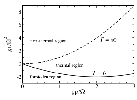
Let us now investigate what the coupled macroscopic equations for the action and energy density can give at high temperatures. The behavior of the system can be viewed in the plane (more precisely, half-plane, as by construction), shown in Fig. 7. It is convenient to measure and in the natural units and . The properties of the grand canonical equilibrium mapping define three regions in the plane Rasmussen2000 . (i) The region below the line is forbidden: for each fixed value of total norm , the Hamiltonian (3) has an absolute minimum , so lower energies are not allowed. This is precisely the line. For weak disorder, , the line is close to that for the clean case , , and it is the latter one that is shown in Fig. 7. (ii) The region between the line and the line (the latter is determined by regardless of the disorder) corresponds to the usual thermal states: for any in this region the corresponding values of and can be found. (iii) The region above the line corresponds to the so-called non-thermal states of the system, which cannot be described by the grand-canonical ensemble with a non-negative temperature (negative temperatures are not allowed in the thermodynamic limit , since the upper bound for the Hamiltonian for a fixed total norm is ). For the disorder-free chain, it has been shown that in the non-thermal region the “excess energy” tends to condense into localized discrete breathers Rasmussen2000 ; Rumpf2004 ; Johansson2004 ; Rumpf2007 ; Rumpf2008 ; Rumpf2009 ; Iubini2013 .
The present work is concerned with the regime
| (84) |
In fact, the conditions of validity discussed in Sec. IV, imply even stronger restrictions, but for the discussion of this subsection inequalities (84) suffice. Namely, they ensure that the thermodynamic relations can be approximated by (see Appendix E for details)
| (85) |
where . Inequalities (84) imply , which justifies the expansion in the powers of .
The region of the plane defined by inequalities (84) is the lower vicinity of the line in the left part of Fig. 7. Neglecting the nonlinear frequency shifts, as in Sec. VI.2, would correspond to approximating the two parabolas by the straight tangents at , , and studying the dynamics of on the horizontal tangent to the line, . However, to check how important is the coupling between the action and the energy transport, one should keep the in the energy and the off-diagonal matrix elements of . The inequality is not sufficient to establish which of the two contributions to in Eq. (83) is more important: the first one is proportionl to the small factor , the second one to , and becomes more important than the first only at . Thus, both contrubutions are kept in the equations below.
Instead of the temperature, it is convenient to introduce the excess energy
| (86) |
Then, using Eq. (62), Eq. (83) (which is valid to the order , other corrections being of the order due to the even-odd symmetry in the frequencies), Eq. (85) [which should be inverted keeping the terms ], the estimate [a natural guess from Eqs. (60), (74), (VI.2), which will be verified numerically in Sec. VII], and neglecting terms which have relative smallness , one arrives at the following closed system of equations:
| (87a) | |||||
| (87b) | |||||
Two conclusions can be drawn from these equations. (i) The second term in has a relative smallness compared to the first. Thus, in the regime defined by inequalities (84) the use of the nonlinear diffusion equation (1) for the density alone is justified. (ii) If one prepares an initial condition with some profile , while everywhere, then , so the system is pulled into the non-thermal region. This fact can be easily understood: if the system tends to an equilibrium state with , , the equilibrium values must be given by the spatial averages of the initial and ; the convexity of the line ensures .
Interestingly, Eqs. (87a) and (87b) remain mathematically correct even for , i. e., in the non-thermal region where the reasoning of this section, based on the assumption of local thermal equilibrium, is not supposed to be valid. Formally, the origin of such behavior can be traced to the fact that Eq. (78) still determines a stationary solution of the kinetic equation even for , . This stationary solution, however, no longer corresponds to the maximum of the entropy; the latter is reached in a state with one discrete breather on top of the background Rumpf2004 . Nevertheless, this true equilibrium state will be reached only at very long times Johansson2004 . This should be especially true in the regime considered here, when the excess energy is small. At not too long times, the system may equilibrate near a transient metastable state with negative temperature. A straightforward analysis of Eqs. (87a), (87b), linearized around a homogeneous solution , , shows that this homogeneous solution is stable regardless of the sign of . Such equilibration has been observed numerically Mulansky2009 . Thus, in the non-thermal region Eqs. (87a), (87b) describe the system dynamics near such a metastable state.
VII Numerical results for the transport coefficients
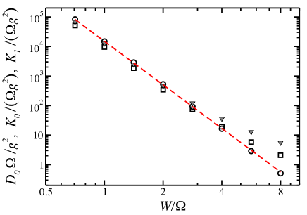
The transport coefficients , , have been evaluated numerically from Eqs. (60), (74), and (VI.2). The frequency functions were approximated by boxes of finite width, as discussed in Sec. III.5), and the absence of dependence of the results on has been checked. The dimensionless combinations , , depend only on the dimensionless disorder strength, and the results of their numerical evaluation are shown in Fig. 8. At weak disorder, they can be fitted by
| (88) |
One feature of these results is that . This follows naturally from Eqs. (60), (74), (VI.2), if the main contribution comes from modes with frequencies . Also, comparing Eqs. (88) and (34a), one can see that , which follows from Eqs. (60) and (28), if the main contribution to and comes from modes with .
Does the observed dependence of or on the disorder strength have a simple explanation? If one assumes that the typical value of for modes located on the same localization segment scales as with some exponent , and the summation over in Eq. (28) gives a factor , then . Several values for the exponent , ranging from 2 to 4, have been suggested in the literature Shepelyansky1994 ; Imry1995 ; Frahm1995 ; Ponomarev1997 ; Krimer2010 ; Michaely2012 . In particular, numerical evaluation of the averages , , gave Frahm1995 or Krimer2010 . The result of the present work, from Eq. (34a), is reproduced if one assumes . The discrepancy is probably due to the fact that in Refs. Frahm1995 ; Krimer2010 for all eigenmodes modes were considered, regardless of their frequencies. At the same time, the sums in Eqs. (28), (60) are contributed only by those modes for which the frequency mismatch is small, and even within this subset there are correlations between the overlaps and the mode frequencies, as illustrated in Appendix A.3. Moreover, even though the points on Fig. 8 seem to fall well on a straight line, one cannot exclude that Eq. (88) still does not represent the true asymptotic behavior at weak disorder (see the discussion in Sec. IV.3).
The value of determined from Eq. (60) can be compared to the one extracted from the rate of wave packet spreading obtained by direct numerical integration of Eq. (2) in Ref. Laptyeva2010 . Eq. (1) has a well-known self-similar solution Zeldovich1950 ; Barenblatt1952 (see also Ref. Vazquez for a comprehensive review):
| (89) |
and for . This solution is parametrized by the total norm , which is determined by the initial conditions and remains conserved in time. Eq. (89) also represents the long-time asymptotics of the solution of Eq. (1) for any positive compact initial condition. The second moment for the wave packet described by Eq. (89),
| (90) |
can be directly compared with the numerical result of Ref. Laptyeva2010 for , averaged over the disorder realizations,
for and . This gives . It should be noted, however, that as the logarithm is a concave function, so this value is likely to underestimate . At the same time, evaluation of Eq. (60) for gives . This can be considered a reasonable agreement, given the fact that is on the borderline of the weak-disorder regime. In addition, from the data of Ref. Laptyeva2010 it is seen that the wave packet expansion with starts to slow down at , that is, at the average density in the packet , which also agrees with the low-density boundary in Fig. 5.
VIII Conclusions
In this paper, we have studied the discrete nonlinear Schrödinger equation in the presence of weak on-site disorder. The nonlinearity was assumed, on the one hand, to be sufficiently weak so that the eigenmodes of the linear problem remain well-resolved, but on the other hand, to be sufficiently strong, so that the dynamics of the eigenmode amplitudes is chaotic for almost all modes. It was shown that in this regime, the slow dynamics of the eigenmode intensities can be described by a master equation of the Fokker-Planck type. Limits of applicability of the master equation approach have been investigated in detail.
Focusing on the transport of conserved quantities (action/norm and energy) on macroscopic length and time scales at high temperature, from the master equation we have derived explicit expressions for the macroscopic transport coefficients in terms of the wave functions and frequencies of the eigenmodes of the linear problem. Evaluation of these expressions was performed numerically for different disorder strengths. Analysis of the coupled macroscopic equations for the norm and energy densities have shown that in the considered regime (weak disorder, moderately weak nonlinearity, and high temperature) the effect of the energy transport on the transport of action (norm) can be neglected, so that the norm density satisfies a closed macroscopic equation, which is the nonlinear diffusion equation with the density-dependent diffusion coefficient . The numerical value of , obtained from the present theory, is in reasonable agreement with the result of the direct numerical integration of the original nonlinear Schrödinger equation Laptyeva2010 .
The density dependence of the diffusion coefficient , obtained in the present work, translates into the subdiffusive spreading of an initially localized wave packet with the second moment growing as . It is known from numerical simulations, that at lower densities or longer times this asymptotics should slow down to , which would mean . Construction of a quantitative theory for this latter regime remains a challenge.
IX Acknowledgements
The author is grateful to B. Altshuler, S. Flach, V. Kravtsov, and A. Pikovsky for stimulating discussions.
Appendix A Statistics for a linear one-dimensional chain
In this Appendix, several quantities are calculated for the linear eigenvalue problem (5) with the flat box distribution for .
A.1 Mode spectral density and localization length
The average -mode spectral density per unit length is defined as
| (91) |
where the function should be approximated by a peak of finite width, which should be set to zero after the limit is taken. The -mode frequency spacing within one localization length is then .
In the weak-disorder limit, for most frequencies , the density of modes can be well approximated by that of the clean chain. is straightforwardly calculated,
| (92) |
and has square-root type singularities at the band edges, . The main effect of weak disorder is to smear these singularities, as seen from the numerical results shown in Fig. 9(a). The smearing occurs on the frequency scale .
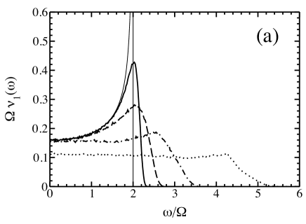
Given the analytical expression, Eq. (92), the two-mode spectral density can also be calculated analytically:
| (93) | |||||
expressed in terms of the complete elliptic integral . The singularities at are logarithmic, i. e., weaker than for , as they are smeared by the convolution.
The three-mode spectral density,
| (94) |
is regular at , , while at it has a cusp, . Thus, in the most relevant interval , is almost a constant. For it monotonously decreases to zero. In general, have weaker singularities for larger , and in the limit one obains the Gaussian shape of due to the central limit theorem.
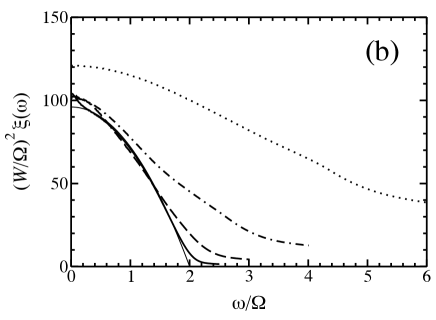
For the localization length, the following analytical expression is available in the weak disorder limit Thouless1979 :
| (95) |
As seen from Fig. 9(b), for this expression works well for most values of , except for the band edges and the band center. The latter behavior is a consequence of the well-known anomaly Gorkov1976 ; Czycholl1981 ; Kappus1981 ; Schomerus2003 ; Deych2003 ; Kravtsov2010 . Other anomalies at frequencies corresponding to wave vectors being rational multiples of Derrida1984 ; Kravtsov2011 are beyond the numerical precision of the present calculation.
A.2 Fluctuations of nonlinear frequency shifts
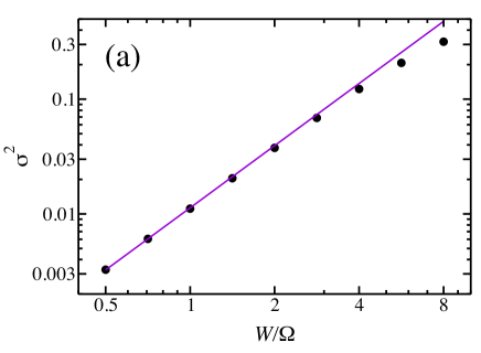
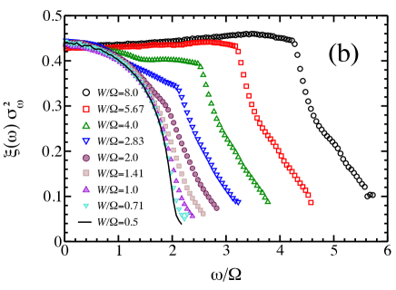
| In this subsection, we present the results for the average relative dispersion of the nonlinear frequency shifts, which was defined in Eq. (13) as the average over all eigenmodes , | |||
| (96a) | |||
| as well as for | |||
| (96b) | |||
| which restricts the average to eigenmodes at a given frequency . | |||
The numerical results for are shown in Fig. 10(a). At weak disorder, the dependence on the disorder strength can be fitted by the expression
| (97) |
that is, . This dependence is slightly weaker than expected from the simple reasoning of Sec. III.1. The reason for this can be understood by looking at the frequency-resolved fluctuation, Eq. (96b), scaled by the localization length at the same frequency, , plotted in Fig. 10(b). At , the curves clearly show different behavior in two distinct frequency intervals, as was also observed in Ref. JohriBhatt . At the curves show a clear tendency to collapse on a single universal curve, but the limit is reached quite slowly. Thus, the asymptotics is expected to set in at small , corresponding to extremely large . Similar behavior in the statistics of values of a single eigenfunction was observed in Ref. Kravtsov2011 . This is also in agreement with discussion of the relaxation rates in Sec. IV.3.
A.3 Correlations between frequencies and overlaps
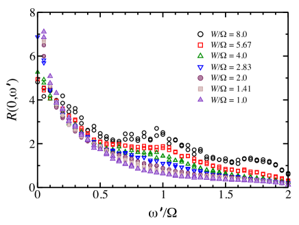
To see how the overlaps which contribute to are correlated with the frequencies of the corresponding modes, we calculate the following quantity:
| (98) |
where if , and in the opposite case ( is introduced in order to take care of the symmetry by choosing the one which is closer to ). Thus defined represents the relative weight with which partner modes at some frequency contribute to , with the normalization
| (99) |
for different disorder strengths is shown in Fig. 11. At weak disorder, the symbols have a tendency to collapse on a single curve. At , has a singularity at . The present data are not sufficient to establish its precise character (power-law or logarithmic); one can only conclude that the singularity is not stronger than , and is thus integrable. At the same time, in the disorder-free system, the singularity is , as was seen in Sec. IV.3. Again, as in Sec. IV.3 and Appendix A.2, it appears that the values of disorder corresponding for which the results are presented in Fig. 11 are still too large to be in the true weak-disorder limit.
Appendix B Damped oscillator subject to noise
Consider a single oscillator, described by the complex amplitude which satisfies the equation of motion,
| (100) |
where is the frequency of linear oscillations, and is the anharmonicity. The solution of Eq. (100) is
| (101) |
Let now the oscillator be subject to a white noise and friction:
| (102) |
where the noise amplitudes satisfy
| (103) |
measures the strength of the noise, and is the friction coefficient. Writing , one can introduce the probability distribution function in the complex plane of , and write down the Fokker-Planck equation, corresponding to the Langevin equation (102):
| (104) |
If is interpreted as the density in a cloud of particles, the first two lines of Eq. (104) correspond to the clockwise rotation of the cloud around the origin, the third line to the uniform squeezing towards the origin, and the last line to the uniform spread of the cloud. In the action-angle variables, , the same equation becomes
| (105) |
where we introduced [which is the equilibrium average value of , since the stationary solution of Eq. (105) is ], and plays the role of the action-dependent diffusion coefficient. Upon averaging over the phase , Eq. (105) becomes identical to Eq. (26).
Appendix C Nonlinear oscillator under a quasi-periodic force
Consider a single oscillator, described by the complex amplitude which satisfies the equation of motion,
| (106) |
where the real are the amplitude and the phase of the th external force oscillating at frequency . Without loss of generality, we assume , . When will the motion of this oscillator be chaotic?
Let us first analyze the case when only one term is present. Substituting
| (107) |
we arrive at equations of motion which have a Hamiltonian form:
| (108a) | |||
| (108b) | |||
| (108c) | |||
where we denoted . The stationary points are located at or , and can be found from the cubic equation,
| (109) |
At , there is only one elliptic stationary point at , and the phase portrait of the oscillator motion in the plane has the same topology as in the absence of the external force. At , two more stationary points appear at , one elliptic and one hyperbolic. The phase portrait of the oscillator in this case is shown in Fig. 12(a). It has a separatrix, which corresponds to the standard case of the nonlinear resonance Chirikov1979 ; Zaslavsky .
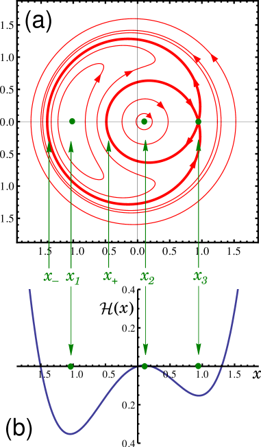
Let us study this separatrix in more detail. As the stationary points are at (corresponding to ) it is convenient to study the Hamiltonian as a function of the dimensionless variable :
| (110) |
whose behavior is determined by a single dimensionless parameter . Let be the stationary points, i. e., the roots of the cubic equation (the prime indicates the derivative). Noting that changes sign at , we obtain that the points are elliptic, while the point is hyperbolic.
The points at which the separatrix crosses the negative real semiaxis of (that is, ) should be found from the equation . Since
| (111) |
they are given by . Both solutions are negative when , which is the case when .
An exact analytic expression for (which depends on the dimensionless parameter ) is not available. Analyzing the cubic parabola , one can see that satisfy
| (112) |
where are the roots at , the points are the extrema of , and is the solution of . Numerically, can be efficiently found by the Newton’s method starting from , respectively. It turns out that is well approximated by
| (113) |
whose relative error does not exceed 1.4% in the whole available range . It is this approximate expression that is used in the numerical calculation.
Let us now consider several forces acting on the oscillator. Treating each of them separately, for those of them which have and thus produce a separatrix, we can define the values (the action corresponding to the hyperbolic point) and (the actions corresponding to the points where the separatrix passes through ). If the separatrices are well separated, that is, the width of the separatrix is much smaller than the typical distance for different , the different resonances do not interfere. If the opposite happens, that is, for some the intervals and overlap, the motion becomes chaotic, and the chaotic region roughly corresponds to the interval . This is essentially the Chirikov’s criterion Chirikov1959 ; Chirikov1979 ; Zaslavsky .
Thus, for each normal mode , whose action is determined by the initial condition and the anharmonicity is given by , we determine the forces and the corresponding separatrix intervals . If among various terms at least two distinct triples can be found such that , the mode is counted as chaotic.
Appendix D Decoupling of higher moments
Let us neglect the correlations in zero approximation, , and check whether in the next approximation the cumulant for is smaller than the main average . The master equation, Eq. (LABEL:master=), gives
| (114) |
containing a double sum. At the same time, for the main average, , from Eq. (44) one straightforardly obtains an expression involving a triple sum. Since each summation involves a large number of terms, the cumulant is smaller then the main average.
Appendix E Thermodynamics at high temperatures
Let us denote for brevity. Then the partition function,
| (115) |
for the Hamiltonian
| (116) |
can be straightforwardly calculated in the high-temperature limit:
| (117) |
where is the second moment of the disorder potential, is the chain length, and the limit is taken at constant . Differentiating this expression with respect to and , we obtain the norm and energy densities,
| (118a) | |||
| (118b) | |||
The limit is reached at the line . Since the temperature (otherwise the partition function diverges, as the Hamiltonian is not bounded from above), the states of the system for which are non-Gibbsian, that is, it is impossible to find and which would produce such and in the grand canonical ensemble Rasmussen2000 . It is convenient to introduce the amount of “non-thermal” energy in the system,
| (119) |
Let us now see what thermodynamic relations are obtained from Eq. (45), the equilibrium solution of the kinetic equation (44) which neglects the nonlinear shifts. Expanding in , we obtain
| (120a) | |||
| (120b) | |||
where the average of is calculated by noting that it is the trace of the square of the linear operator on the right-hand side of Eq. (5). Eqs. (120a), (120b) differ from Eqs. (118a), (118b) by the absence of the nonlinear terms proportional to , but also by the coefficients at . The origin of this latter difference can be traced back to non-vanishing correlations, when . Indeed, Eq. (118b) keeps track of all correlations, while Eq. (120b) follows from Eq. (44) which was obtained by neglecting correlations. Still, the relative error of Eq. (120b) with respect to Eq. (118b) is , which was precisely the justification for neglecting the correlations in Eq. (44).
If we use the equilibrium solution which includes the nonlinear frequency shifts, Eq. (79), and calculate the average action and energy densities, it reproduces Eq. (118a) for , while for it gives
| (121) |
This expression differs from Eq. (118b) by the numerical coefficients at (discussed above), and at . The latter produces a relative error in the coefficient at .
Appendix F Spatio-temporal smoothing
Let us express in Eq. (47) in terms of the normal mode wave functions and amplitudes :
| (122) |
Only terms with survive the convolution with when . Then, averaging over , we obtain
| (123) |
In the spatial sum, we expand around to the second order:
| (124) |
The second term vanishes by the definition of , and in the last term the first factor gives , while the sum over is .
Appendix G Toy model of an electric -cirquit

It is instructive to see how the formalism of Sec. V works for a very simple toy model, that of an electric -circuit, shown in Fig. 13. The dynamics of the charge on the th capacitor is governed by the equation
| (128) |
Indeed, is the electrostatic potential on the upper plate of the th capacitor, and is the current flowing through the resistor between the capacitors and . In equilibrium, the potential is constant along the chain.
For the simple model of Eq. (128), the exact relation between the current and the macroscopic charge density or potential gradient can be derived straightforwardly. Indeed, noticing that in a stationary situation the currents through all resistors should be the same, we the potential drop is determined by
| (129) |
so the potential differents between any two capacitors and is given by
| (130) |
Taking , from this we can calculate the macroscopic potential gradient
| (131) |
where is the average resistance,
| (132) |
The “thermodynamic equation of state”, relating the charge density to the potential, is
| (133) |
where is the average capacitance, defined analogously to . As a result, we obtain the sought relation between the current and the gradient of the potential or charge density:
| (134) |
Let us now see how the approach of Sec. V works for Eq. (128). The macroscopic density and current are defined as
| (135a) | |||
| (135b) | |||
To find the current response to a small gradient of the potential, let us look for a stationary solution of Eq. (128) in the form
| (136) |
with the requirement . The corrections can be found from the equations
| (137) |
which are satisfied when
| (138) |
The constant should be chosen to ensure . This condition yields and the solution
| (139) |
With this solution, the current is obtained from Eq. (135b), which gives .
References
- (1) M. B. Gertsenshtein and V. B. Vasil’ev, Theory Probab. Appl. 4, 391 (1959).
- (2) N. F. Mott and W. D. Twose, Adv. Phys. 10, 107 (1961).
- (3) G. M. Zaslavsky, Chaos in Dynamic Systems, (Harwood Academic Publishers, Newark, 1985).
- (4) A. J. Lichtenberg and M. A. Lieberman, Regular and Chaotic Dynamics (Springer-Verlag, New York, 1992), 2nd ed.
- (5) D. L. Shepelyansky, Phys. Rev. Lett. 70, 1787 (1993).
- (6) M. I. Molina, Phys. Rev. B 58, 12547 (1998).
- (7) G. Kopidakis, S. Komineas, S. Flach, and S. Aubry, Phys. Rev. Lett. 100, 084103 (2008).
- (8) A. S. Pikovsky and D. L. Shepelyansky, Phys. Rev. Lett. 100, 094101 (2008).
- (9) J. Fröhlich, T. Spencer, and C. E. Wayne, J. Stat. Phys. 42, 247 (1986).
- (10) M. Johansson, G. Kopidakis, and S. Aubry, Europhys. Lett. 91, 50001 (2010).
- (11) V. Oganesyan, A. Pal, and D. A. Huse, Phys. Rev. B 80, 115104 (2009).
- (12) D. M. Basko, Ann. Phys. 326, 1577 (2011).
- (13) A. Pikovsky and S. Fishman, Phys. Rev. E 83, 025201(R) (2011).
- (14) M. Mulansky, K. Ahnert, A. Pikovsky and D. L. Shepelyansky, J. Stat. Phys. 145, 1256 (2011).
- (15) D. M. Basko, Phys. Rev. E 86, 036202 (2012).
- (16) Ch. Skokos, I. Gkolias, and S. Flach, Phys. Rev. Lett. 111, 064101 (2013).
- (17) Y. Lahini, A. Avidan, F. Pozzi, M. Sorel, R. Morandotti, D. N. Christodoulides, and Y. Silberberg, Phys. Rev. Lett. 100, 013906 (2008).
- (18) E. Lucioni, B. Deissler, L. Tanzi, G. Roati, M. Zaccanti, M. Modugno, M. Larcher, F. Dalfovo, M. Inguscio, and G. Modugno, Phys. Rev. Lett. 106, 230403 (2012).
- (19) S. Fishman, Y. Krivolapov, and A. Soffer, Nonlinearity 25, R53 (2012).
- (20) S. Flach, D. O. Krimer, and Ch. Skokos, Phys. Rev. Lett. 102, 024101 (2009).
- (21) Ch. Skokos and S. Flach, Phys. Rev. E 82, 016208 (2010).
- (22) T. V. Laptyeva, J. D. Bodyfelt, D. O. Krimer, Ch. Skokos and S. Flach, EPL 91, 30001 (2010).
- (23) J. D. Bodyfelt, T. V. Laptyeva, Ch. Skokos, D. O. Krimer, and S. Flach, Phys. Rev. E 84, 016205 (2011).
- (24) G. Benettin, J. Fröhlich, and A. Giorgilli, Commun. Math. Phys. 119, 95 (1988).
- (25) W.-M. Wang and Z. Zhang, J. Stat. Phys. 134, 953 (2009).
- (26) S. Fishman, Y. Krivolapov, and A. Soffer, Nonlinearity 22, 2861 (2009).
- (27) M. Mulansky, K. Ahnert, and A. Pikovsky, Phys. Rev. E 83, 026205 (2011).
- (28) M. Mulansky and A. Pikovsky, New J. Phys. 15, 053015 (2013).
- (29) M. Mulansky, arXiv:1310.8116.
- (30) E. Michaely and S. Fishman, Phys. Rev. E 85, 046218 (2012).
- (31) V. E. Zakharov, V. S. L’vov, and G. E. Falkovich, Kolmogorov Spectra of Turbulence I – Wave Turbulence (Springer-Verlag, Berlin, 1992).
- (32) S. Flach, Chem. Phys. 375, 548 (2010).
- (33) M. Mulansky and A. Pikovsky, EPL 90, 10015 (2010).
- (34) S. Flach, M. Ivanchenko, and N. Li, Pramana J. Phys. 77, 1007 (2011).
- (35) T. V. Laptyeva, J. D. Bodyfelt, and S. Flach, Physica D 256–257, 1 (2013).
- (36) F. Huveneers, Nonlinearity 26, 837 (2013).
- (37) K. Ø. Rasmussen, T. Cretegny, P. G. Kevrekidis, and N. Grønbech-Jensen, Phys. Rev. Lett. 84, 3740 (2000).
- (38) S. Iubini, S. Lepri, and A. Politi, Phys. Rev. E 86, 011108 (2012).
- (39) V. E. Kravtsov and V. I. Yudson, Ann. Phys. 326, 1672 (2011).
- (40) N. Bilas and N. Pavloff, Eur. Phys. J. D 40, 387 (2006).
- (41) V. Gurarie, G. Refael, and J. T. Chalker, Phys. Rev. Lett. 101, 170407 (2008).
- (42) L. D. Landau and E. M. Lifshitz, Quantum mechanics, non-relativistic theory (Pergamon Press, Oxford, 1991).
- (43) D. J. Thouless, in Ill-condensed matter, ed. by G. Toulouse and R. Balian (North-Holland, Amsterdam, 1979).
- (44) D. M. Basko, I. L. Aleiner, and B. L. Altshuler, Ann. Phys. (N.Y.) 321, 1126 (2006).
- (45) I. L. Aleiner, B. L. Altshuler, and G. V. Shlyapnikov, Nature Phys. 6, 900 (2010).
- (46) A. A. Gogolin, V. I. Melnikov and É. I. Rashba, Zh. Eksp. Teor. Fiz. 69, 327 (1975) [Sov. Phys. JETP 42, 168 (1975)].
- (47) D. M. Basko, Phys. Rev. Lett. 91, 206801 (2003).
- (48) B. Rumpf, Phys. Rev. E 69, 016618 (2004).
- (49) M. Johansson and K. Ø. Rasmussen, Phys. Rev. E 70 066610 (2004).
- (50) B. Rumpf, Europhys. Lett. 78, 26001 (2007).
- (51) B. Rumpf, Phys. Rev. E 77, 036606 (2008).
- (52) B. Rumpf, Physica D 238, 2067 (2009).
- (53) S. Iubini, R. Franzosi, R. Livi, G.-L. Oppo and A. Politi, New Journal of Physics 15, 023032 (2013).
- (54) M. Mulansky, K. Ahnert, A. Pikovsky, and D. L. Shepelyansky Phys. Rev. E 80, 056212 (2011).
- (55) D. L. Shepelyansky, Phys. Rev. Lett. 73, 2607 (1994).
- (56) Y. Imry, Europhys. Lett. 30, 405 (1995).
- (57) K. Frahm, A. Müller-Groeling, J.-L. Pichard, and D. Weinmann, Europhys. Lett. 31, 169 (1995).
- (58) I. V. Ponomarev and P. G. Silvestrov, Phys. Rev. B 56, 3742 (1997).
- (59) D. O. Krimer and S. Flach, Phys. Rev. E 82, 046221 (2010).
- (60) Y. B. Zel’dovich and A. Kompaneets, in Collected papers of the 70th Anniversary of the Birth of Academician A. F. Ioffe, Moscow, 1950.
- (61) G. I. Barenblatt, Prikl. Mat. Mekh. 16, 67 (1952).
- (62) J. L. Vazquez, The porous medium equation: mathematical theory (Oxford University Press, 2007).
- (63) L. P. Gorkov and O. N. Dorokhov, Solid State Commun. 20, 789 (1976)
- (64) G. Czycholl, B. Kramer, and A. MacKinnon, Z. Phys. B 43, 5 (1981).
- (65) M. Kappus and F. Wegner, Z. Phys. B 45, 15 (1981).
- (66) H. Schomerus and M. Titov, Phys. Rev. B 67, 100201(R) (2003).
- (67) L. I. Deych, M. V. Erementchouk, A. A. Lisyansky, and B. L. Altshuler, Phys. Rev. Lett. 91, 096601 (2003).
- (68) V. E. Kravtsov and V. I. Yudson, Phys. Rev. B 82, 195120 (2010).
- (69) B. Derrida and E. Gardner, J. Phys. (Paris) 45, 1283 (1984)
- (70) S. Johri and R. N. Bhatt, Phys. Rev. Lett. 109, 076402 (2012).
- (71) B. V. Chirikov, Phys. Rep. 52, 263 (1979).
- (72) B.V.Chirikov, J. Nucl. Energy Part C: Plasma Phys. 1, 253 (1960).