DMUS–MP–13/19, PUPT-2456, LPTENS 13/23

We analyze $\mathcal{N}=1$ theories on $S^{5}$ and $S^{4}\times S^{1}$, showing how their partition functions can be written in terms of a set of fundamental 5d holomorphic blocks. We demonstrate that, when the 5d mass parameters are analytically continued to suitable values, the $S^{5}$ and $S^{4}\times S^{1}$ partition functions degenerate to those for $S^{3}$ and $S^{2}\times S^{1}$. We explain this mechanism via the recently proposed correspondence between 5d partition functions and correlators with underlying $q$-Virasoro symmetry. From the $q$-Virasoro 3-point functions, we axiomatically derive a set of associated reflection coefficients, and show that they can be geometrically interpreted in terms of Harish-Chandra $c$-functions for quantum symmetric spaces. We link these particular $c$-functions to the types appearing in the Jost functions encoding the asymptotics of the scattering in integrable spin-chains, obtained taking different limits of the XYZ model to XXZ-type.

1 Introduction

The study of supersymmetric gauge theories on compact manifolds has attracted much attention in recent years. After the seminal work by Pestun Pestun:2007rz , the method of supersymmetric localization has been applied to compute partition functions of theories formulated on compact manifolds of various dimensions. A comprehensive approach to rigid supersymmetry in curved backgrounds has been also proposed Festuccia:2011ws .

In this paper we focus on 5d $\mathcal{N}=1$ theories. Exact results for partition functions of $\mathcal{N}=1$ theories on $S^{5}$ and $S^{4}\times S^{1}$ were derived in Kallen:2012cs ; Hosomichi:2012ek ; Kallen:2012va ; Kim:2012ava ; Imamura:2012bm ; Lockhart:2012vp ; Kim:2012qf ; Minahan:2013jwa and Kim:2012gu ; Terashima:2012ra ; Iqbal:2012xm . In the case of the squashed $S^{5}$, the partition function $Z_{S^{5}}$ was shown to localize to a matrix integral of classical, 1-loop and instanton contributions. The latter in turn comprises of three copies of the equivariant instanton partition function on $\mathbb{R}^{4}\times S^{1}$ Nekrasov:2002qd ; Nekrasov:2003rj with an appropriate identification of the equivariant parameters, each copy corresponding to the contribution at a fixed point of the Hopf fibration of $S^{5}$ over $\mathbb{CP}^{2}$. The $S^{4}\times S^{1}$ case is similar with the instanton partition function consisting of the product of two copies of the equivariant instanton partition function on $\mathbb{R}^{4}\times S^{1}$, corresponding to the fixed points at the north and south poles of $S^{4}.$

Our first result is the observation that, by manipulating the classical and 1-loop part to a form which respects the symmetry dictated by the gluing of the instanton factors, it is possible to rewrite $Z_{S^{5}}$ and $Z_{S^{4}\times S^{1}}$ in terms of the same fundamental building blocks, which we name 5d holomorphic blocks ${\cal B}^{5d}$. In formulas:

$$Z_{S^{5}}=\int d\sigma~{}\Big{|}\Big{|}{\cal B}^{5d}\Big{|}\Big{|}^{3}_{S}\,,\qquad Z_{S^{4}\times S^{1}}=\int d\sigma~{}\Big{|}\Big{|}{\cal B}^{5d}\Big{|}\Big{|}^{2}_{id}\,,$$

where the brackets $\Big{|}\Big{|}\ldots\Big{|}\Big{|}^{3}_{S}$ and $\Big{|}\Big{|}\ldots\Big{|}\Big{|}^{2}_{id}$ glue respectively three and two 5d holomorphic blocks, as described in details in the main text. This result is very reminiscent of the 3d case where $S^{2}\times S^{1}$ and $S^{3}$ partition functions were shown to factorize in terms of the same set of building blocks, named 3d holomorphic blocks ${\cal B}^{3d}_{\alpha}$, glued with different pairings Pasquetti:2011fj ; hb :

$$Z_{S^{3}}=\sum_{\alpha}~{}\Big{|}\Big{|}{\cal B}^{3d}_{\alpha}\Big{|}\Big{|}^{2}_{S}\,,\qquad Z_{S^{2}\times S^{1}}=\sum_{\alpha}~{}\Big{|}\Big{|}{\cal B}^{3d}_{\alpha}\Big{|}\Big{|}^{2}_{id}\,.$$

Holomorphic blocks in three dimensions were identified with solid tori or Melving cigars $M_{q}=D^{2}\times S^{1}$ partition functions, the subscripts $id$, $S$ refer to the way blocks are fused which was shown to be consistent with the decomposition of $S^{2}\times S^{1}$ and $S^{3}$ in solid tori glued by $id$ and $S$ elements in $SL(2,\mathbb{Z})$. The index $\alpha$ labels the SUSY vacua of the semiclassical $\mathbb{R}^{2}\times S^{1}$ theory but it also turns out to run over a basis of solutions to certain difference operators which annihilates 3d blocks and 3d partition functions Dimofte:2011py ; Dimofte:2011ju ; hb .

In fact, the similarity between the structure of 5d and 3d partition functions is not just a coincidence, but it is due to a deep relation between the two theories. For example we consider the 5d $\mathcal{N}=1$ SCQCD with $SU(2)$ gauge group and four flavors on $S^{4}\times S^{1}$ and $S^{5}$ and show that, when the masses are analytically continued to certain values, 5d partition functions degenerate to 3d partition functions of the SQED with $U(1)$ gauge group and four flavors respectively on $S^{2}\times S^{1}$ and $S^{3}$. Schematically:

$$Z_{S^{5}}^{SCQCD}=\int d\sigma~{}\Big{|}\Big{|}{\cal B}^{5d}\Big{|}\Big{|}^{3}_{S}\,\longrightarrow\,Z_{S^{3}}^{SQED}=\sum_{\alpha}~{}\Big{|}\Big{|}{\cal B}^{3d}_{\alpha}\Big{|}\Big{|}^{2}_{S}\,,$$

and

$$Z_{S^{4}\times S^{1}}^{SCQCD}=\int d\sigma~{}\Big{|}\Big{|}{\cal B}^{5d}\Big{|}\Big{|}^{2}_{id}\,\longrightarrow\,Z_{S^{2}\times S^{1}}^{SQED}=\sum_{\alpha}~{}\Big{|}\Big{|}{\cal B}^{3d}_{\alpha}\Big{|}\Big{|}^{2}_{id}\,,$$

where the 5d $id$ and $S$ gluings reduce to the corresponding pairing for 3d theories introduced in hb . The mechanisms that leads to this degeneration is the fact that, upon analytic continuation of the masses, 1-loop terms develop poles which pinch the integration contour. Partition functions then receive contribution from the residues at the poles trapped along the integration contour. This result is roughly the compact version of the degeneration of the instanton partition function to the vortex partition function of simple surface operators Alday:2009fs ; Dimofte:2010tz ; Kozcaz:2010af ; Bonelli:2011fq , since $S^{2}\times S^{1}$ and $S^{3}$ are codimension-2 defects inside respectively $S^{4}\times S^{1}$ and $S^{5}$.

The fact that when analytically continuing flavor parameters partition functions degenerate to sum of terms annihilated by difference operators is quite general, for example this is the case also for the 4d superconformal index Gaiotto:2012xa . In the case of the degeneration of 4d instanton partition functions to surface operator vortex counting, this mechanism has been related, via the AGT correspondence, to the analytic continuation of a primary operator to a degenerate primary in Liouville correlators Alday:2009fs . We can offer a similar interpretation of the rich structure of the degeneration of 5d partition functions in the context of the correspondence, proposed in Nieri:2013yra , between 5d partition functions and correlators with underlying symmetry given by a deformation of the Virasoro algebra known as ${\cal V}ir_{q,t}$. In Nieri:2013yra two families of such correlators, dubbed respectively $S$ and $id$-correlators, were constructed by means of the bootstrap approach using the explicit form of degenerate representations of ${\cal V}ir_{q,t}$ as well as an ansatz for the pairings of the ${\cal V}ir_{q,t}$ chiral blocks, generalizing the familiar holomorphic-antiholomorphic square. The two families of correlators differ indeed by the pairing of the blocks and are endowed respectively with 3-point functions $C_{S}$ and $C_{id}$. In Nieri:2013yra it was checked that $Z_{S^{5}}$ and $Z_{S^{4}\times S^{1}}$ partition functions of the 5d $\mathcal{N}=1$ SCQCD with $SU(2)$ gauge group and $N_{f}=4$ are captured respectively by 4-point $S$ and $id$-correlator on the 2-sphere.

In this paper we provide another check showing that 1-point torus correlators capture the ${\cal N}=1^{*}$ $SU(2)$ theory, that is the theory of a vector multiplet coupled to one adjoint hyper. We also reinterpret and clarify the degeneration mechanisms of 5d partition functions in terms of fusion rules of degenerate ${\cal V}ir_{q,t}$ primaries. In particular, the pinching of the integration contour for the 5d partition functions is described in detail using the language of ${\cal V}ir_{q,t}$ correlators.

As pointed out in Zamolodchikov:1995aa , 3-point functions can also be used to define the reflection coefficients, which in turn encode very important information about the theory. In the case of Liouville theory a semiclassical reflection coefficient, which is perturbative in the Liouville coupling constant $b_{0}$, can be obtained from a “first quantized”-type analysis. In the so-called mini-superspace approximation Seiberg , one can solve the Schrödinger equation for the zero-mode of the Liouville field which scatters from an exponential barrier. The same equation appears when studying the radial part of the Laplacian in horospheric coordinates on the hyperboloid $SL(2,\mathbb{C})/SU(2)$ (Lobachevsky space) (see for instance Mironov ; OlshanetskyRogov ; OlshanetskyPerelomov and further references in the main text).

In this case, the reflection coefficient can be expressed as a ratio of so-called Harish-Chandra $c$-functions for the root system of the underlying $\mathfrak{sl}(2)$ Lie algebra. In fact, this procedure is purely group-theoretic (see also GerasimovMarshakovOlshanetskyShatashvili ; GerasimovMarshakovMorozovOlshanetskyShatashvili ) and can be generalized to the case of quantum group deformations. The results appear to be given in terms of products of factors associated to the root decomposition of the relevant (quantum) algebra. These factors, in turn, are given in terms of certain special functions which are typically Gamma functions and generalizations thereof FreundZabrodinII . An important observation in GerasimovKharchevMarshakovMironovMorozovOlshanetsky is that one can obtain the exact non-perturbative Liouville reflection coefficient by considering the affine version of the $\mathfrak{sl}(2)$ algebra. While the non-affine version produces the semiclassical reflection coefficient, the affinization procedure, which includes the contributions from the affine root (equivalently, from the infinite tower of affine levels), generates the exact non-pertubative result. In a sense, the affinization procedure plays the role of a “second quantization”, restoring the non-perturbative dependence in the Liouville parameter $1/b_{0}$.

Inspired by this remarkable observation we checked whether our exact reflection coefficients, for the two types of geometries/correlator-pairings considered in Nieri:2013yra , could be reproduced by a similar affinization procedure, starting from a suitable choice of Harish-Chandra $c$-functions. We found that this is indeed the case. Our reflection coefficients can be obtained by affinizing the ratio of Harish-Chandra functions given in terms of $q$-deformed Gamma functions $\Gamma_{q}$ and double Gamma functions $\Gamma_{2}$ for the $id$- and $S$-pairing, respectively. The $\Gamma_{q}$ function appears in the study of the quantum version of the Lobachevsky space, which involves the quantum algebra $U_{q}(\mathfrak{sl}(2))$. The appearance of the $\Gamma_{2}$ function is harder to directly relate to a specific quantum group construction, even thought it has been conjectured to be part of a hierarchy of integrable structures FreundZabrodinII .

It is quite remarkable to observe that the affinization mechanisms works for the situation in object in this paper precisely as it did for Liouville theory. In particular, it is highly non-trivial that such procedure is capable of restoring the $SL(3,\mathbb{Z})$ invariance of the 5d $S$-pairing after the infinite resummation. We believe that this occurrence deserves further investigations.

To shed more light on the type of special functions appearing in our reflection coefficients, we consider scattering of excitations in integrable spin-chains, which are prototypical representatives in the universality classes of 2-dimensional integrable systems. We find that the special functions in our reflection coefficients are indeed typical of scattering processes between particle-like excited states in different regimes of the XXZ system, obtained as limiting cases from the XYZ spin-chain. In particular, the id-pairing produces $\Gamma_{q}$ functions that characterize the scattering in the antiferromagnetic regime of the XXZ spin-chain, while the S-pairing produces $\Gamma_{2}$ functions, related to the scattering on the XXZ chain in its disordered regime (and also, for instance, in the Sine-Gordon model). The link between reflection coefficients, Harish-Chandra functions and scattering matrices of integrable systems is in essence the one anticipated in the work of Freund and Zabrodin (see for instance FreundZabrodinII and further references in the main text). In this sense, we can establish a direct connection between the axiomatic properties of the $q$-deformed systems underlying gauge theory partition functions, their semiclassical images consisting of quantum mechanical reflections from a potential barrier, their geometric pictures in terms of group theory data, and the exact analysis of 2-dimensional integrable hierarchies.

The underlying presence of the $q$-deformed Virasoro symmetry is strongly suggestive that the properties of the $q$-conformal blocks and of the emerging integrable systems should be intimately tied together. In particular, we expect that a significant part will be played by the $q$-deformed Knizhnik-Zamolodchikov equation FrenkelReshetikhin ; Lukyanov:1992sc , and, correspondingly, by the integrable form-factor equations Smirnov ; LashkevichPugai .

The appearance of the XXZ spin-chain in connection with reflection coefficients is not surprising since, as it was shown in Nieri:2013yra , the 3-point functions $C_{S}$ and $C_{id}$ were ultimately derived from 3d $\mathcal{N}=2$ theories whose SUSY vacua can be mapped to eigenstates of spin-chain Hamiltonians ns1 ; ns2 . For further results in this direction see lc1 ; lc2 ; gk ; gaddegukovputrovwalls .

2 5d holomorphic blocks

In this section we study 5d ${\cal N}=1$ theories formulated on the squashed $S^{5}$ and on $S^{4}\times S^{1}$. We begin by recording the expressions obtained in the literature for the partition functions $Z_{S^{5}}$ and $Z_{S^{4}\times S^{1}}$. We then show that $Z_{S^{5}}$ and $Z_{S^{4}\times S^{1}}$ can be decomposed in terms of 5d holomorphic blocks ${\cal B}^{5d}$. We also show how $S^{5}$ and $S^{4}\times S^{1}$ partition functions degenerate to $S^{3}$ and $S^{2}\times S^{1}$ partition functions when masses are analytically continued to suitable values.

2.1 Squashed $S^{5}$ partition functions and 5d holomorphic blocks

In a series of papers Kallen:2012cs ; Hosomichi:2012ek ; Kallen:2012va ; Kim:2012ava ; Imamura:2012bm ; Lockhart:2012vp ; Kim:2012qf ; Minahan:2013jwa the 5d ${\cal N}=1$ supersymmetric gauge theory has been formulated on $S^{5}$ with squashing parameters $\omega_{1},\omega_{2},\omega_{3}$, and the partition function has been shown to localize to the integral over the zero-mode of the vector multiplet scalar $\sigma$ which takes value in the Cartan subalgebra of the gauge group, which we take to be $SU(N)$ with generators $T_{a}$ normalized as $\text{Tr}_{R}(T_{a}T_{b})=C_{2}(R)\delta_{ab}$, with $C_{2}(F)=1/2$ for the fundamental. The integrand includes a classical factor ${Z}_{\text{cl}}(\sigma)$, a 1-loop factor ${Z}_{\text{1-loop}}(\sigma,\vec{M})$ and an instanton factor ${Z}_{\text{inst}}(\sigma,\vec{M})$

$$Z_{S^{5}}=\int d\sigma~{}{Z}_{\text{cl}}(\sigma){Z}_{\text{1-loop}}(\sigma,\vec{M}){Z}_{\text{inst}}(\sigma,\vec{M})\,,$$ (1)

where we schematically denote by $\vec{M}$ all mass parameters of the theory and the explicit expressions of the factors depend on the field content of the 5d ${\cal N}=1$ theory under consideration.

The instanton partition function ${Z}_{\text{inst}}(\sigma,\vec{M})$ receives contributions from the three fixed points of the Hopf fibration over the $\mathbb{CP}^{2}$ base, and, as show in Lockhart:2012vp ; Kim:2012qf , takes the following factorized form:

$$Z_{\text{inst}}(\sigma,\vec{M})=\Big{|}\Big{|}{\cal Z}_{\text{inst}}\Big{|}\Big{|}^{3}_{S}\,,$$ (2)

where ${\cal Z}_{\text{inst}}$ coincides with the equivariant instanton partition function on ${\mathbb{R}}^{4}\times S^{1}$ Nekrasov:2002qd ; Nekrasov:2003rj with Coulomb and mass parameters appropriately rescaled and with equivariant parameters $\epsilon_{1}=\frac{e_{1}}{e_{3}}$ and $\epsilon_{2}=\frac{e_{2}}{e_{3}}$:

$${\cal Z}_{\text{inst}}={\cal Z}^{\mathbb{R}^{4}\times S^{1}}_{\text{inst}}\left(\frac{i\sigma}{e_{3}},\frac{\vec{m}}{e_{3}};\frac{e_{1}}{e_{3}},\frac{e_{2}}{e_{3}}\right)\,,$$ (3)

where

$$m_{j}=iM_{j}+E/2\,,\qquad j=1,\cdots,N_{f}\,,$$ (4)

and $E=\omega_{1}+\omega_{2}+\omega_{3}$. We also introduced the notation:

$$\displaystyle\Big{|}\Big{|}(\dots)\Big{|}\Big{|}^{3}_{S}:=(\ldots)_{1}(\ldots)_{2}(\ldots)_{3}\,,$$ (5)

where the sub-indices $1,2,3$ refer to the following identification of the parameters $e_{1},e_{2},e_{3}$ to the squashing parameters $\omega_{1},\omega_{2},\omega_{3}$ in each sector:

$$\displaystyle\begin{array}[]{|c|ccc|}\hline\cr&\quad e_{1}&\quad e_{2}&\quad e_{3}\\ \hline\cr 1&\omega_{3}&\omega_{2}&\omega_{1}\\ 2&\omega_{1}&\omega_{3}&\omega_{2}\\ 3&\omega_{1}&\omega_{2}&\omega_{3}\\ \hline\cr\end{array}$$ (10)

Explicitly we have:

$$\displaystyle\left({\cal Z}_{\rm inst}\right)_{1}={\cal Z}^{\mathbb{R}^{4}\times S^{1}}_{\rm inst}\left(\frac{i\sigma}{\omega_{1}},\frac{\vec{m}}{\omega_{1}};\frac{\omega_{2}}{\omega_{1}},\frac{\omega_{3}}{\omega_{1}}\right)\,, \,\left({\cal Z}_{\rm inst}\right)_{2}={\cal Z}^{\mathbb{R}^{4}\times S^{1}}_{\rm inst}\left(\frac{i\sigma}{\omega_{2}},\frac{\vec{m}}{\omega_{2}};\frac{\omega_{1}}{\omega_{2}},\frac{\omega_{3}}{\omega_{2}}\right)\,,$$ (11)

$$\!\!\!\!\!\!\!\!\!\!\!\!\!\!\!\!\!\!\!\!\!\!\!\!\!\!\!\!\!\!\!\!\!\!\!\!\!\!\!\!\!\!\!\!\!\!\!\!\!\left({\cal Z}_{\rm inst}\right)_{3}={\cal Z}^{\mathbb{R}^{4}\times S^{1}}_{\rm inst}\left(\frac{i\sigma}{\omega_{3}},\frac{\vec{m}}{\omega_{3}};\frac{\omega_{1}}{\omega_{3}},\frac{\omega_{2}}{\omega_{3}}\right)\,.$$

Notice that since the instanton partition function can be expressed in terms of the parameters

$$q=e^{2\pi ie_{1}/e_{3}}\,,\quad t=e^{2\pi ie_{2}/e_{3}}\,,$$ (12)

the pairing defined in eq. (5) enjoys an $SL(3,\mathbb{Z})$ symmetry which acts S-dualizing the couplings $q$ and $t$.

The classical factor contains the contribution of the Yang-Mills action given by

$${Z}_{\rm cl}(\sigma)=e^{\frac{2\pi i}{\omega_{1}\omega_{2}\omega_{3}g^{2}}\,\text{Tr}(\sigma^{2})}=e^{-\frac{2\pi i}{\omega_{1}\omega_{2}\omega_{3}g^{2}2C_{2}(ad)}\sum_{\alpha}[i\alpha(\sigma)]^{2}}$$ (13)

where we denoted by $\alpha$ a root of the Lie algebra of the gauge group and we used that $2C_{2}(ad)\sum_{\rho}\rho(\sigma)^{2}=\sum_{\alpha}\alpha(\sigma)^{2}$. We can try to bring this term in the $SL(3,\mathbb{Z})$ factorized form as the instanton contribution. We begin by rewriting the classical term by means of the Bernoulli polynomial $B_{33}$, defined in appendix A.1, as

$${Z}_{\rm cl}(\sigma)=\prod_{\alpha}e^{-\frac{2\pi i}{3!}\left[B_{33}\left(i\alpha(\sigma)+\frac{1}{g^{2}2C_{2}(ad)}+\frac{E}{2}\right)-B_{33}\left(\frac{1}{g^{2}2C_{2}(ad)}+\frac{E}{2}\right)\right]}.$$ (14)

Each factor in the above expression can in turn be factorized thanks to the following identity fv

$$\displaystyle e^{-\frac{2\pi i}{3!}B_{33}(z)} = \prod_{k=1}^{3}\Gamma_{q,t}\left(\frac{z}{e_{3}}\right)_{k}=\Big{|}\Big{|}\Gamma_{q,t}\left(\frac{z}{e_{3}}\right)\Big{|}\Big{|}^{3}_{S}\,,$$ (15)

where the elliptic gamma function $\Gamma_{q,t}$ is defined in appendix A.4. Hence by applying the identity (15) to each Bernoulli factor we obtain:

$$\displaystyle{Z}_{\rm cl}(\sigma)=\Big{|}\Big{|}{\cal Z}_{\rm cl}\Big{|}\Big{|}^{3}_{S}\,,$$ (16)

with

$$\displaystyle{\cal Z}_{\rm cl}=\prod_{\alpha}\frac{\Gamma_{q,t}\left(\frac{1}{e_{3}}\left(i\alpha(\sigma)+\frac{1}{g^{2}2C_{2}(ad)}+\frac{E}{2}\right)\right)}{\Gamma_{q,t}\left(\frac{1}{e_{3}}\left(\frac{1}{g^{2}2C_{2}(ad)}+\frac{E}{2}\right)\right)}\,.$$ (17)

We can therefore write the partition function as:

$$\displaystyle Z_{S^{5}}=\int~{}d\sigma~{}{Z}_{\text{1-loop}}(\sigma,\vec{M})~{}\Big{|}\Big{|}{\cal F}\Big{|}\Big{|}^{3}_{S}\,,$$ (18)

with

$${\cal F}={\cal Z}_{\rm cl}\,{\cal Z}_{\text{inst}}\,,$$ (19)

where ${\cal Z}_{\rm cl}$ and ${\cal Z}_{\text{inst}}$ are given respectively in (17) and (3).

We can give another representation of the partition function where we bring also the 1-loop contribution to an $SL(3,\mathbb{Z})$ factorized form as in Lockhart:2012vp . We remind that a vector multiplet contributes to the partition function with

$${Z}^{\text{vect}}_{\text{1-loop}}(\sigma)=\prod_{\alpha>0}S_{3}(i\alpha(\sigma))S_{3}(E+i\alpha(\sigma))\,,$$ (20)

while a hyper multiplet of mass $M$ and representation $R$ gives

$${Z}^{\text{hyper}}_{\text{1-loop}}(\sigma,M,R)=\prod_{\rho\in R}S_{3}\left({i\rho(\sigma)}+iM+\frac{E}{2}\right)^{-1}\,,$$ (21)

where $S_{3}$ is the triple sine function defined in appendix A.2. Using the relation (159), the vector multiplet contribution can be written as

$$\displaystyle{Z}^{\text{vect}}_{\text{1-loop}}(\sigma) = \prod_{\alpha>0}e^{-\frac{\pi i}{3!}{[B_{33}(i\alpha(\sigma))+B_{33}(i\alpha(\sigma)+E)]}}(1-e^{\frac{2\pi i}{\omega_{1}}[i\alpha(\sigma)]})(1-e^{\frac{2\pi i}{\omega_{2}}[i\alpha(\sigma)]})(1-e^{\frac{2\pi i}{\omega_{3}}[i\alpha(\sigma)]})$$ (22)

$$\times\,\prod_{k=1}^{3}(te^{\frac{2\pi i}{e_{3}}[i\alpha(\sigma)]};q,t)_{k}(qe^{\frac{2\pi i}{e_{3}}[i\alpha(\sigma)]};q,t)_{k}\,,$$

where $(z;q,t)=\prod_{i,j\geq 0}(1-zq^{i}t^{j})$ denotes the double $(q,t)$-factorial, while the sub-index $k$ refers to the way $q,t$ defined in (12) are related to the squashing parameters according to (10). Each factor $(te^{\frac{2\pi i}{e_{3}}[i\alpha(\sigma)]};q,t)_{k}(qe^{\frac{2\pi i}{e_{3}}[i\alpha(\sigma)]};q,t)_{k}$ can in turn be identified with the 1-loop vector multiplet contribution to the ${\mathbb{R}}^{4}\times S^{1}$ theory Nekrasov:2002qd ; Nekrasov:2003rj ; Alday:2009aq appropriately rescaled, and with equivariant parameters as in (12). We can equivalently factorize the vector multiplet 1-loop term in the following more compact form:

$$\displaystyle Z^{\text{vect}}_{\text{1-loop}}(\sigma) = \prod_{\alpha}e^{-\frac{\pi i}{3!}B_{33}(i\alpha(\sigma))}\prod_{k=1}^{3}(e^{\frac{2\pi i}{e_{3}}{[}i\alpha(\sigma){]}};q,t)_{k}.$$ (23)

Analogously, the hyper multiplet factor can be written as

$$\displaystyle{Z}^{\text{hyper}}_{\text{1-loop}}(\sigma,M,R) = \prod_{\rho\in R}e^{\frac{\pi i}{3!}B_{33}(i\rho(\sigma)+iM+\frac{E}{2})}\prod_{k=1}^{3}(e^{\frac{2\pi i}{e_{3}}[i\rho(\sigma)+iM+\frac{E}{2}{]}};q,t)_{k}^{-1}\,,$$ (24)

where $(e^{\frac{2\pi i}{e_{3}}{[}i\rho(\sigma)+iM+\frac{E}{2}{]}};q,t)^{-1}$ can be identified with the 1-loop hyper multiplet contribution to the ${\mathbb{R}}^{4}\times S^{1}$ partition function Nekrasov:2002qd ; Nekrasov:2003rj ; Alday:2009aq . The full 1-loop contribution to the partition function as can be therefore written as

$$Z_{\text{1-loop}}(\sigma,\vec{M})=\prod_{R}\prod_{\begin{subarray}{c}\alpha\\ \rho\in R\end{subarray}}e^{-\frac{\pi i}{3!}[B_{33}(i\alpha(\sigma))-B_{33}(i\rho(\sigma)+m_{R})]}\prod_{k=1}^{3}\frac{(e^{\frac{2\pi i}{e_{3}}[i\alpha(\sigma)]};q,t)_{k}}{(e^{\frac{2\pi i}{e_{3}}[i\rho(\sigma)+m_{R}]};q,t)_{k}}$$ (25)

where $m_{R}=iM_{R}+E/2$ is the mass of a multiplet in the representation $R$. If we consider (pseudo) real representations, for each weight $\rho$ there is the opposite weight $-\rho$, in which case the Bernoulli sum to a quadratic polynomial which can be easily factorized in terms of elliptic Gamma functions as we did for the classical term. In fact, in this case the Bernoulli from the 1-loop factor will amounts to a renormalization of the gauge coupling constant. To see this, let us consider $N_{f}$ fundamentals of mass $M_{f}$ and $N_{f}$ anti-fundamentals of mass $\bar{M}_{f}$, with $f=1,\ldots,N_{f}$, and $N_{a}$ adjoints of mass $M_{a}$, $a=1,\ldots,N_{a}$. The total contribution from 1-loop Bernoulli terms is (up to a $\sigma$-independent constant)

$$e^{-\frac{2\pi i}{\omega_{1}\omega_{2}\omega_{3}}\frac{\sum_{\alpha}[i\alpha(\sigma)]^{2}}{2C_{2}(ad)}\left[\frac{E}{4}N_{f}-\frac{1}{4}\sum_{f}(m_{f}+\bar{m}_{f})+C_{2}(ad)(\frac{E}{2}(N_{a}-1)-\sum_{a}m_{a})\right]}\,,$$ (26)

since $\sum_{\rho}\rho(\sigma)=0$ for $SU(N)$. Comparing the above expression with the classical action (13), it is easy to obtain the factorized version of (26) by shifting the gauge coupling constant in (17), according to

$$\frac{1}{g^{2}}\rightarrow\frac{1}{g^{2}}+\frac{E}{4}N_{f}-\frac{1}{4}\sum_{f}(m_{f}+\bar{m}_{f})+C_{2}(ad)\left(\frac{E}{2}(N_{a}-1)-\sum_{a}m_{a}\right)\,.$$ (27)

Therefore also the total 1-loop contribution admits a factorized form:

$$\displaystyle{Z}_{\rm 1-loop}(\sigma,\vec{M})=\Big{|}\Big{|}{\cal Z}_{\text{1-loop}}\Big{|}\Big{|}^{3}_{S}\,.$$ (28)

Putting all together we can finally write (up to constant prefactors):

$$Z_{S^{5}}=\int d\sigma~{}\Big{|}\Big{|}{\cal B}^{5d}\Big{|}\Big{|}^{3}_{S}\,,$$ (29)

where ${\cal B}^{5d}$, the 5d holomorphic block, is defined as

$${\cal B}^{5d}={\cal Z}_{\text{1-loop}}~{}{\cal Z}_{\text{cl}}~{}{\cal Z}_{\text{inst}}\,.$$ (30)

It is important to note the way we factorize 1-loop and classical terms is not unique. We have seen an example of this for the vector multiplet contribution. We will now see more precisely how to track this ambiguity in an example.

The $SU(2)$ superconformal QCD

We consider the superconformal QCD (i.e. SCQCD) with $SU(2)$ gauge group. In this case, the Coulomb branch parameter can be written as $\sigma=i\bigl{(}\begin{smallmatrix}a_{1}&0\\ 0&a_{2}\end{smallmatrix}\bigr{)}$ with $a_{1}=-a_{2}=a$ and the vector multiplet is coupled to four fundamental hyper multiplets with masses $M_{f}$, $f=1,2,3,4$. The total 1-loop contribution is given by:

$$Z_{\rm 1-loop}(a,\vec{M})=\frac{S_{3}\left(a_{1}-a_{2}\right)S_{3}\left(a_{2}-a_{1}\right)}{\prod_{f}S_{3}\left(a_{1}+m_{f}\right)S_{3}\left(a_{2}+m_{f}\right)}\,.$$ (31)

Collecting the $B_{33}$ factors coming from the factorization of the $S_{3}$ functions in (31) we find:

$$B_{33}(2a)+B_{33}(-2a)-\sum_{f}[B_{33}(a+m_{f})+B_{33}(-a+m_{f})]=-\frac{6a^{2}}{\omega_{1}\omega_{2}\omega_{3}}\sum_{f}m_{f}+const\,,$$ (32)

where the constant denotes $a$-independent terms. We then combine 1-loop and the classical Yang-Mills action

$$Z_{\text{cl}}(a)=e^{-\frac{2\pi i}{\omega_{1}\omega_{2}\omega_{3}}\frac{a^{2}}{\tilde{g}^{2}}}\,,$$

where $\tilde{g}^{2}=g^{2}/2$ obtaining:

$$Z_{\text{cl}}(a)~{}{Z}_{\text{1-loop}}(a,\vec{M})=e^{-\frac{2\pi ia^{2}}{\omega_{1}\omega_{2}\omega_{3}}\left(\frac{1}{\tilde{g}^{2}}-\frac{1}{2}\sum_{f}m_{f}\right)}\prod_{k=1}^{3}\frac{(e^{\frac{2\pi i}{e_{3}}[\pm 2a]};q,t)_{k}}{\prod_{f=1}^{4}(e^{\frac{2\pi i}{e_{3}}[\pm a+m_{f}]};q,t)_{k}}\,,$$ (33)

where for compactness we have employed the shorthand notation $f(\pm a)=f(a)f(-a)$. The next step is to write the exponential as a sum of $B_{33}$,

$$e^{-\frac{2\pi ia^{2}}{\omega_{1}\omega_{2}\omega_{3}}\left(\frac{1}{\tilde{g}^{2}}-\frac{1}{2}\sum_{f}m_{f}\right)}=\frac{e^{-\frac{2\pi i}{3!}B_{33}(\pm a+\frac{1}{\tilde{g}^{2}}-\frac{1}{2}\sum_{f}m_{f}+\kappa)}}{e^{-\frac{2\pi i}{3!}B_{33}(\pm a+\kappa)}}\times\frac{e^{-\frac{4\pi i}{3!}B_{33}(\kappa)}}{e^{-\frac{4\pi i}{3!}B_{33}(\frac{1}{\tilde{g}^{2}}-\frac{1}{2}\sum_{f}m_{f}+\kappa)}}\,.$$ (34)

In this expression the coefficient $\kappa$ appearing only on the R.H.S. is completely arbitrary and can be identified with the ambiguity of the factorization. Finally we apply the identity (15) to each Bernoulli factor in (34) and obtain the SQCD 5d holomorphic blocks:

$$\mathcal{B}^{\rm 5d}=\frac{(e^{\frac{2\pi i}{e_{3}}[\pm 2a]};q,t)}{\prod_{f}(e^{\frac{2\pi i}{e_{3}}[\pm a+m_{f}]};q,t)}\cdot\frac{\Gamma_{q,t}\left(\frac{\pm a+1/\tilde{g}^{2}-\sum_{f}m_{f}/2+\kappa}{e_{3}}\right)}{\Gamma_{q,t}\left(\frac{\pm a+\kappa}{e_{3}}\right)}\cdot\mathcal{Z}_{\text{inst}}\,.$$ (35)

2.2 $S^{4}\times S^{1}$ partition functions and 5d holomorphic blocks

The partition functions for 5d ${\cal N}=1$ supersymmetric gauge theory on $S^{4}\times S^{1}$ has been computed in Kim:2012gu ; Terashima:2012ra ; Iqbal:2012xm and reads

$$\displaystyle Z_{S^{4}\times S^{1}} = \int d\sigma~{}{Z}_{\text{1-loop}}(\sigma,\vec{M})~{}{Z}_{\text{inst}}(\sigma,\vec{M})\,,$$ (36)

where $\sigma$ is the Coulomb branch parameter. The instanton part receives contributions from the fixed points at north and south poles of the $S^{4}$ and can be written as

$$Z_{\text{inst}}=\Big{|}\Big{|}{\cal Z}_{\text{inst}}\Big{|}\Big{|}^{2}_{id}\,,$$ (37)

where as before ${\cal Z}_{\rm inst}$ coincides with the equivariant instanton partition function on ${\mathbb{R}}^{4}\times S^{1}$ with Coulomb and mass parameters appropriately rescaled, and a particular parameterization of the equivariant parameters:

$${\cal Z}_{\text{inst}}(\sigma,\vec{m})={\cal Z}^{\mathbb{R}^{4}\times S^{1}}_{\text{inst}}\left(\frac{i\sigma}{e_{3}},\frac{\vec{m}}{e_{3}};\frac{e_{1}}{e_{3}},\frac{e_{2}}{e_{3}}\right)\,,$$ (38)

with $m_{j}=iM_{j}+Q_{0}/2$ and $Q_{0}=b_{0}+1/b_{0}$. We also introduced the 5d $id$-pairing defined as

$$\displaystyle\Big{|}\Big{|}(\dots)\Big{|}\Big{|}^{2}_{id}:=(\ldots)_{1}(\ldots)_{2}\,,$$ (39)

where the 1,2 sub-indices means that the $e_{1},e_{2},e_{3}$ parameters assume the following values:

$$\displaystyle\begin{array}[]{|c|ccc|}\hline\cr&\quad e_{1}&\quad e_{2}&\quad e_{3}\\ \hline\cr 1&b_{0}^{-1}&b_{0}&2\pi i/\beta\\ 2&b_{0}^{-1}&b_{0}&-2\pi i/\beta\\ \hline\cr\end{array}$$ (43)

with $\beta$ the circumference of $S^{1}$ and $b_{0}$ the squashing parameter of $S^{4}$.

Due to the property (181) the elliptic Gamma function satisfies $\Big{|}\Big{|}\Gamma_{q,t}(z)\Big{|}\Big{|}^{2}_{id}=1$ and the classical term ${\cal Z}_{\text{cl}}$ defined in eq. (17) “squares” to one:

$$\Big{|}\Big{|}{\cal Z}_{\text{cl}}\Big{|}\Big{|}_{id}^{2}=1\,.$$ (44)

We can therefore write

$$\displaystyle Z_{S^{4}\times S^{1}} = \int d\sigma~{}{Z}_{\text{1-loop}}(\sigma,\vec{M})~{}\Big{|}\Big{|}{\cal F}\Big{|}\Big{|}^{2}_{id}\,,$$ (45)

with ${\cal F}$ defined in eq. (19).

The 1-loop contributions of vector and hyper multiplets are given respectively by

$${Z}^{\text{vect}}_{\text{1-loop}}(\sigma)=\prod_{\alpha>0}\Upsilon^{\beta}\left(i\alpha(\sigma)\right)\Upsilon^{\beta}\left(-i\alpha(\sigma)\right)\,,$$ (46)

and

$${Z}^{\text{hyper}}_{\text{1-loop}}(\sigma,M,R)=\prod_{\rho\in R}\Upsilon^{\beta}\left({i\rho(\sigma)+iM}+\frac{Q_{0}}{2}\right)^{-1}\,,$$ (47)

where $\Upsilon^{\beta}$ is defined in appendix A.3. Also in this case it is possible to bring the 1-loop term in a factorized form. Indeed if we use again that $\Big{|}\Big{|}\Gamma_{q,t}(z)\Big{|}\Big{|}^{2}_{id}=1$ we can write

$${Z}^{\text{vec}}_{\text{1-loop}}(\sigma)=\Big{|}\Big{|}{\cal Z}^{\text{vec}}_{\text{1-loop}}\Big{|}\Big{|}^{2}_{id}\,,\qquad{Z}^{\text{hyper}}_{\text{1-loop}}(\sigma,\vec{M})=\Big{|}\Big{|}{\cal Z}^{\text{hyper}}_{\text{1-loop}}\Big{|}\Big{|}^{2}_{id}\,,$$ (48)

with ${\cal Z}^{\text{vec}}_{\text{1-loop}},{\cal Z}^{\text{hyper}}_{\text{1-loop}}$ coinciding with the corresponding factors obtained from the factorization of 1-loop terms on $S^{5}$, which implies that

$$Z_{S^{4}\times S^{1}}=\int d\sigma~{}\Big{|}\Big{|}{\cal B}^{5d}\Big{|}\Big{|}^{2}_{id}\,.$$ (49)

Hence we surprisingly discover that for a given theory, the $S^{5}$ and $S^{4}\times S^{1}$ partition functions can be factorized in terms of the same 5d blocks ${\cal B}^{5d}$. This is very reminiscent to what happens in 3d, where the partition function for $S^{3}_{b}$ and $S^{2}\times S^{1}$ can be expressed via the same blocks, paired in two different ways hb .

It would be very interesting to test whether partition functions on more general 5-manifolds can be engineered by fusing our ${\cal B}^{5d}$ blocks with suitable gluings.

2.3 Degeneration of $5d$ partition functions

An interesting feature of $S^{5}$ and $S^{4}\times S^{1}$ partition functions (1), (36) is that for particular values of the masses 1-loop factors develop poles which pinch the integration contour. The partition functions can then be defined via a meromorphic analytic continuation which prescribes to take the residues at the poles trapped along the integration path. Here we will consider a particular example, the $SU(2)$ theory with four fundamental hyper multiplets with masses $M_{f}$, $f=1,\ldots,4$ on $S^{5}$. In this case when two of the masses, say $M_{1},M_{2}$, satisfy the following condition:

$$M_{1}+M_{2}=i(\omega_{3}+E)\qquad{\rm or}\qquad m_{1}+m_{2}=-\omega_{3}\,,$$ (50)

where $m_{i}$ are defined in (4), the partition function receives contribution only from two pinched poles located at

$$a_{1}=m_{1}=-m_{2}-\omega_{3}=-a_{2}\,,\qquad a_{1}=m_{1}+\omega_{3}=-m_{2}=-a_{2}\,.$$ (51)

This is reminiscent of the degeneration of a Liouville theory 4-point correlation function when one of the momenta is analytically continued to a degenerate value. The AGT setup explains that the degeneration limit corresponds on the gauge theory side to the reduction of 4d partition functions to simple surface operator partition functions Alday:2009fs ; Dimofte:2010tz ; Kozcaz:2010af ; Bonelli:2011fq . In particular the $S^{4}$ SCQCD partition function, in this limit, reduces to its codimension-2 BPS defect theory, the $S^{2}$ SQED Higgs branch partition function Doroud:2012xw ; Benini:2012ui . Therefore we expect that, when the masses are analytically continued to the values (50), the squashed $S^{5}$ SCQCD partition function will degenerate to its codimension-2 defect theory, the 3d SQED defined on the squashed 3-sphere $S_{b}^{3}$ which we record below. The $S^{3}_{b}$ Higgs branch partition function of the $U(1)$, $\mathcal{N}=2$ theory with 2 charge plus and 2 charge minus chirals, takes the following form Pasquetti:2011fj :

$$Z_{S^{3}_{b}}=\sum_{i=1,2}G^{(i)}_{\rm cl}G^{(i)}_{\rm 1-loop}\Big{|}\Big{|}\mathcal{Z}^{(i)}_{V}\Big{|}\Big{|}^{2}_{S}\,,$$ (52)

where the sum runs over the two SUSY vacua of theory and

$$G^{(i)}_{\rm cl}=e^{-2\pi i\xi m^{3d}_{i}}\,,\qquad G^{(i)}_{\rm 1-loop}=\prod_{j,k=1,2}\frac{s_{b}(m^{3d}_{j}-m^{3d}_{i}+iQ/2)}{s_{b}(\tilde{m}^{3d}_{k}-m^{3d}_{i}-iQ/2)}\,,\quad j\neq i\,,$$ (53)

$$\displaystyle\mathcal{Z}^{(i)}_{V}=\sum_{n\geq 0}\prod_{j,k=1,2}\frac{(y_{k}x_{i}^{-1};q)_{n}}{(qx_{j}x_{i}^{-1};q)_{n}}(u^{3d})^{n}\,,$$ (54)

where $b$ is the squashing parameter of the ellipsoid, $Q=b+1/b$, and $s_{b}$ is the double sine function defined in appendix A.1. The vortex partition functions $\mathcal{Z}^{(i)}_{V}$ are basic hypergeometric functions defined in (193) with coefficients:

$$\displaystyle x_{i} = e^{2\pi bm^{3d}_{i}},\quad y_{i}=e^{2\pi b\tilde{m}^{3d}_{i}},\quad z^{3d}=e^{2\pi b\xi},\quad q=e^{2\pi ib^{2}}\,,$$

$$\tilde{x}_{i} = e^{2\pi m^{3d}_{i}/b},\quad\tilde{y}_{i}=e^{2\pi\tilde{m}^{3d}_{i}/b},\quad\tilde{z}^{3d}=e^{2\pi\xi/b},\quad\tilde{q}=e^{2\pi i/b^{2}}\,,$$ (55)

and

$$\prod_{j,k=1,2}x_{j}y_{k}^{-1}=r,\quad(u^{3d})=qr^{\frac{1}{2}}(z^{3d})^{-1}\,.$$ (56)

Finally the 3d $S$-pairing is defined as hb :

$$\Big{|}\Big{|}f(x;q)\Big{|}\Big{|}_{S}^{2}=f(x;q)f(\tilde{x};\tilde{q})\,.$$ (57)

We will now show how to reconstruct (52) from the residues of the $S^{5}$ partition function at the pinched poles. We begin by analyzing the SCQCD instanton contribution which is given by:

$$\displaystyle{\cal Z}_{\rm inst}={\cal Z}^{\mathbb{R}^{4}\times S^{1}}_{\rm inst}\left(\frac{\vec{a}}{e_{3}},\frac{\vec{m}}{e_{3}};\frac{e_{1}}{e_{3}},\frac{e_{2}}{e_{3}}\right)=\sum_{\vec{Y}}z^{|\vec{Y}|}\frac{F_{\vec{Y}}(\vec{a},\vec{m})}{V_{\vec{Y}}(\vec{a})}\,,\qquad z=e^{\frac{2\pi i}{e_{3}\tilde{g}^{2}}}\,.$$ (58)

The numerator $F_{\vec{Y}}(\vec{a},\vec{m})$ encodes the contribution of the four hyper multiplets and the denominator $V_{\vec{Y}}(\vec{a})$ is due to the vector multiplet and we refer to appendix B for explicit expressions. As explained in appendix B, when the Coulomb branch parameters take the values $a_{1}=m_{1}=-m_{2}-\omega_{3}=-a_{2}$, the instanton partition function (58) degenerates to a basic hypergeometric function. In particular the instanton partition function in the first sector becomes:

$$\displaystyle\left({\cal Z}_{\rm inst}\right)_{1}={\cal Z}^{\mathbb{R}^{4}\times S^{1}}_{\rm inst}\left(\frac{\vec{a}}{\omega_{1}},\frac{\vec{m}}{\omega_{1}};\frac{\omega_{2}}{\omega_{1}},\frac{\omega_{3}}{\omega_{1}}\right)\ \quad\xrightarrow[(a_{1},a_{2})\rightarrow(m_{1},m_{2}+\omega_{3})]{}\quad\phantom{|}_{2}\Phi_{1}(A,B;C,e^{2\pi i\frac{\omega_{2}}{\omega_{1}}};u)\,,$$

where $A,B,C,u$ parameters are defined in (192) and we replaced $e_{1},e_{2},e_{3}$ in eq. (191) with their values in terms of $\omega_{i}$ in sector 1 as in (10). In sector 2 we use (194) and the appropriate values of $e_{i}$ in terms of $\omega_{i}$ to find:

$$\displaystyle\left({\cal Z}_{\rm inst}\right)_{2}={\cal Z}^{\mathbb{R}^{4}\times S^{1}}_{\rm inst}\left(\frac{\vec{a}}{\omega_{2}},\frac{\vec{m}}{\omega_{2}};\frac{\omega_{1}}{\omega_{2}},\frac{\omega_{3}}{\omega_{2}}\right)\quad\xrightarrow[(a_{1},a_{2})\rightarrow(m_{1},m_{2}+\omega_{3})]{}\quad\phantom{|}_{2}\Phi_{1}(\tilde{A},\tilde{B};\tilde{C},e^{2\pi i\frac{\omega_{1}}{\omega_{2}}};\tilde{u})\,,$$

where the tilde symbol indicates $\omega_{1}\leftrightarrow\omega_{2}$. Finally in sector 3, once the $e_{i}$ are expressed in terms of the $\omega_{i}$ according to (10), all the parameters are rescaled by $\omega_{3}$ yielding a trivial degeneration, as explained in appendix B:

$$\displaystyle\left({\cal Z}_{\rm inst}\right)_{3}={\cal Z}^{\mathbb{R}^{4}\times S^{1}}_{\rm inst}\left(\frac{\vec{a}}{\omega_{3}},\frac{\vec{m}}{\omega_{3}};\frac{\omega_{1}}{\omega_{3}},\frac{\omega_{2}}{\omega_{3}}\right)\quad\xrightarrow[(a_{1},a_{2})\rightarrow(m_{1},m_{2}+\omega_{3})]{}\quad 1\,.$$ (61)

Putting all together we find that

$$\displaystyle\Big{|}\Big{|}{\cal Z}_{\rm inst}\Big{|}\Big{|}^{3}_{S}\quad\xrightarrow[(a_{1},a_{2})\rightarrow(m_{1},m_{2}+\omega_{3})]{}\quad\Big{|}\Big{|}\phantom{|}_{2}\Phi_{1}(A,B;C,e^{2\pi i\frac{\omega_{2}}{\omega_{1}}};u)\Big{|}\Big{|}^{2}_{S}=\Big{|}\Big{|}{\cal Z}^{(1)}_{V}\Big{|}\Big{|}^{2}_{S}\,,$$ (62)

which shows that remarkably the 5d $S$-pairing reduces to the 3d $S$-pairing. Furthermore by identifying the coefficient $A,B,C$ of the basic hypergeometrc function with those of the vortex partition function $\mathcal{Z}^{(1)}_{V}$, as required by last equality in eq. (62), we obtain the following dictionary between 3d and 5d masses:

$$m^{3d}_{1}=-im_{1}\,,\quad m^{3d}_{2}=-im_{2}\,,\quad\tilde{m}^{3d}_{1}=im_{3}\,,\quad\tilde{m}^{3d}_{2}=im_{4}\,,$$ (63)

while by matching the expansion parameters we find

$$i\xi=1/\tilde{g}^{2}\,.$$ (64)

Finally, we also identify

$$\omega_{2}=\frac{1}{\omega_{1}}=b\,.$$ (65)

In complete analogy for the other pole, located at $a_{1}=m_{1}+\omega_{3}=-m_{2}=-a_{2}$, upon using the dictionary (63), we find

$$\displaystyle\Big{|}\Big{|}{\cal Z}_{\rm inst}\Big{|}\Big{|}^{3}_{S}\quad\xrightarrow[(a_{1},a_{2})\rightarrow(m_{1}+\omega_{3},m_{2})]{}\quad\Big{|}\Big{|}\mathcal{Z}^{(2)}_{V}\Big{|}\Big{|}^{2}_{S}\,.$$ (66)

We next consider the 1-loop term given in (31). Since this term has poles when $(a_{1},a_{2})$ take the two values in (51) and since we are only interested in showing that the degeneration of the $S^{5}$ partition function reproduces the $S^{3}_{b}$ partition function up to a prefactor, we evaluate the ratio of the residues at each pole. This ratio is finite and, by using the property (162), it is straightforward to show that it reproduces the ratio of the $S^{3}_{b}$ 1-loop terms in the two SUSY vacua, given in eq. (53):

$$\frac{Z_{\rm 1-loop}\Big{|}_{(a_{1},a_{2})\rightarrow(m_{1},m_{2}+\omega_{3})}}{Z_{\rm 1-loop}\Big{|}_{(a_{1},a_{2})\rightarrow(m_{1}+\omega_{3},m_{2})}}=\frac{G^{(1)}_{\rm 1-loop}}{G^{(2)}_{\rm 1-loop}}\,.$$ (67)

Similarly, it is simple to show that the ratio of the residues of the classical term at the points (51) reproduces the ratio of the $S^{3}_{b}$ classical terms in the two SUSY vacua, given in eq. (53):

$$\frac{Z_{\rm cl}\Big{|}_{(a_{1},a_{2})\rightarrow(m_{1},m_{2}+\omega_{3})}}{Z_{\rm cl}\Big{|}_{(a_{1},a_{2})\rightarrow(m_{1}+\omega_{3},m_{2})}}=e^{-\frac{2\pi i}{\omega_{1}\omega_{2}\omega_{3}}\frac{(m_{1}^{2}-m_{2}^{2})}{\tilde{g}^{2}}}=e^{\frac{2\pi i(m_{1}-m_{2})}{\omega_{1}\omega_{2}\tilde{g}^{2}}}=e^{2\pi i\xi(m_{1}^{\rm 3d}-m_{2}^{\rm 3d})}=\frac{G^{(1)}_{\rm cl}}{G^{(2)}_{\rm cl}}\,,$$ (68)

where we used $m_{1}^{2}-m_{2}^{2}=-\omega_{3}(m_{1}-m_{2})$ and the dictionary (63), (64).

Finally putting all together we obtain the promised result:

$$Z^{SCQCD}_{S^{5}}\quad\xrightarrow[m_{1}+m_{2}=-\omega_{3}]{}\quad\sum_{i}^{2}G^{(i)}_{\rm cl}G^{(i)}_{\rm 1-loop}\Big{|}\Big{|}{\cal Z}^{(i)}_{V}\Big{|}\Big{|}^{2}_{S}=Z^{SQED}_{S^{3}}\,.$$ (69)

Notice that there are two extra choices for the degeneration condition, which would have led to the same result:

$$m_{1}+m_{2}=-\omega_{1}\,,\quad{\rm with}\quad\omega_{2}=\frac{1}{\omega_{3}}=b\,,$$

$$m_{1}+m_{2}=-\omega_{2}\,,\quad{\rm with}\quad\omega_{1}=\frac{1}{\omega_{3}}=b\,.$$ (70)

The three possibilities correspond to choosing one of the three maximal squashed 3-spheres inside the squashed 5-sphere.

In a similar manner, it is possible to show that the partition function of the SCQCD on $S^{4}\times S^{1}$, when two of the masses satisfy the condition

$$m_{1}+m_{2}=-b_{0}\,,$$ (71)

reduces to the SQED partition function on $S^{2}\times S^{1}$:

$$Z^{SCQCD}_{S^{4}\times S^{1}}\quad\xrightarrow[m_{1}+m_{2}=-b_{0}]{}\quad\sum_{i}^{2}G^{(i)}_{\rm cl}G^{(i)}_{\rm 1-loop}\Big{|}\Big{|}{\cal Z}^{(i)}_{V}\Big{|}\Big{|}^{2}_{id}=Z^{SQED}_{S^{2}\times S^{1}}\,,$$ (72)

with the 3d angular momentum fugacity $q$ related to the 5d parameters by $q=e^{\beta/b_{0}}$. Also in this case there is another possible degeneration condition $m_{1}+m_{2}=-\frac{1}{b_{0}}$, which leads to the same result but with the identification $q=e^{\beta b_{0}}$. The two choices, correspond to the two maximal $S^{2}$ inside the squashed $S^{4}$.

2.3.1 Higher degenerations

In the previous section we focused on particular analytic continuations of the 5d masses (51), (71) which degenerate partition functions to a bilinear combination of solutions to basic hypergeometric difference equations. The degeneration mechanism is actually much more general, for example the 1-loop factor of the SCQCD on $S^{5}$ develops poles pinching the integration contour when two of the masses satisfy the following condition:

$$m_{1}+m_{2}=-(n_{1}\omega_{1}+n_{2}\omega_{2}+n_{3}\omega_{3})=-\vec{n}\cdot\vec{\omega}\,,\qquad n_{1},n_{2},n_{3}\in\mathbb{Z}_{+}\,.$$ (73)

In this case the integral localizes to a sum over the following set:

$$\{a^{*}\}:\quad a_{1}=m_{1}+(\vec{n}-\vec{p})\cdot\vec{\omega}\,,\quad a_{2}=m_{2}+\vec{p}\cdot\vec{\omega}\,,$$ (74)

where

$$p_{k}\in\{0,1,\cdots,n_{k}\}\,,\quad k=1,2,3\,.$$ (75)

Evaluating the residues at points (74) we find:

$$\displaystyle Z^{SCQCD}_{S^{5}}\quad\xrightarrow[m_{1}+m_{2}=-\vec{n}\cdot\vec{\omega}]{}\quad\sum_{\{a^{*}\}}\text{ Res}\Big{[}Z_{\rm 1-loop}\Big{]}~{}~{}({\cal F}^{p_{2},p_{3}})_{1}~{}({\cal F}^{p_{3},p_{1}})_{2}~{}({\cal F}^{p_{2},p_{1}})_{3}\,,$$ (76)

where $({\cal F}^{p_{i},p_{j}})$ denotes the value of classical and instanton parts at the pole

$$({\cal F}^{p_{i},p_{j}})_{k}=({\cal Z}^{p_{i},p_{j}}_{\rm cl})_{k}({\cal Z}^{p_{i},p_{j}}_{\rm inst})_{k}\,,\quad{\rm with}\quad i\neq j\neq k=1,2,3\,,$$ (77)

and, as usual, the subscript $k$ means that in each sector we express the $e_{i}$ in terms of the $\omega_{i}$s according to the dictionary (10).

The residue of the instanton contribution is given by:

$${\cal Z}^{p_{2},p_{1}}_{\rm inst}=\sum_{\begin{subarray}{c}Y^{1}=(p_{2},\,p_{1})\\ Y^{2}=(n_{2}-p_{2},\,n_{1}-p_{1})\end{subarray}}\frac{F_{p_{2},p_{1}}}{V_{p_{2},p_{1}}}~{}~{}z^{|\vec{Y}|}\,,$$ (78)

where $F_{p_{2},p_{1}}$ and $V_{p_{2},p_{1}}$ are defined in eqs. (197) and (198). In this case the analytic continuation of the masses restricts the sum to hook Young tableaux with $p_{2}$ rows and $p_{1}$ columns, and with $n_{2}-p_{2}$ rows and $n_{1}-p_{1}$ columns respectively. Furthermore ${\cal Z}^{p_{3},p_{2}}_{\rm inst}$ and ${\cal Z}^{p_{3},p_{1}}_{\rm inst}$ are obtained from ${\cal Z}^{p_{2},p_{1}}_{\rm inst}$ by appropriately renaming/permuting the $p_{i}$.

The value of the classical term ${\cal Z}^{p_{2},p_{1}}_{\rm cl}$ is computed in eqs. (200), (B.1) and the identification of the $p_{i}$ as well as of the $e_{i}$ is like in the instanton case discussed above.

In the next section we will provide an interpretation of the degeneration (76) using the correspondence between the $S^{5}$ SCQCD partition functions and a 4-point $q$-deformed correlators. In particular the analytic continuation (73) will be mapped to the analytic continuation of the momentum of one of the primaries to a higher level degenerate momentum. Clearly the degeneration mechanism of 5d partition functions, due to the analytic continuation of the masses, is not limited to the SCQCD, but it extends to more general quiver gauge theories which via the 5d/$q$-CFT correspondence are mapped to higher point correlation functions.

3 5d partition functions as $q$-correlators

In Nieri:2013yra it was proposed that the 5d partition functions discussed in the previous section are captured by a novel class of correlators, dubbed $q$-correlators or $q$-CFT correlators, with underling $q$-deformed Virasoro symmetry (${\cal V}ir_{q,t}$).

Deformed Virasoro and $\mathcal{W}_{N}$ algebras were introduced in Shiraishi:1995rp ; fr ; Feigin:1995sf ; Awata:1995zk , using a correspondence between singular vectors and multivariable orthogonal symmetric polynomials or using the Wakimoto realization at the critical level. It was also independently shown that the deformed Virasoro algebra emerges as a symmetry in study of the Andrews-Baxter-Forester (ABF) model Lukyanov:1995gs ; Lukyanov:1996qs .

Considering expressions (18) and (45) for partition functions, the match to $q$-correlators requires to identify

$$~{}~{}~{}~{}~{}~{}~{}~{}~{}{Z}_{\text{1-loop}}(\sigma,\vec{m})\,\Leftrightarrow\,{\rm 3-point~{}function~{}factors}\,,$$ (79)

and

$$\,{\cal F}={\cal Z}_{\rm cl}~{}{\cal Z}_{\rm inst}\,\Leftrightarrow\,{\cal V}ir_{q,t}{\rm~{}chiral~{}blocks}\,.$$ (80)

The connection between ${\cal V}ir_{q,t}$ chiral blocks and the 5d Nekrasov instanton function on $\mathbb{R}^{4}\times S^{1}$ was discussed already in the context of the 5d AGT correspondence Awata:2009ur ; Awata:2010yy ; Schiappa:2009cc ; Mironov:2011dk ; Yanagida:2010vz . Our proposal includes the interpretation of ${\cal Z}_{\rm cl}$ as the $q$-deformation of the factor fixed by the conformal Ward identities. Indeed, it is easy to check that since

$$\lim_{e_{3}\to\infty}\Gamma_{q,t}(x/e_{3})\simeq e^{-\frac{2\pi}{3!}B_{33}(x|\vec{e})}\,,$$

in the undeformed Virasoro limit, that is $e_{2}=b_{0}=1/e_{1}$ and $e_{3}=\frac{2\pi i}{\beta}\to\infty$, the classical term ${\cal Z}_{\rm cl}$, upon identifying the Coulomb branch parameter with the internal momentum in the correlator as $\alpha=Q_{0}/2+a$, reduces to:

$$\displaystyle{\cal Z}_{\rm cl}\to e^{-\frac{2\pi i}{e_{1}e_{2}e_{3}}\frac{a^{2}}{\tilde{g}^{2}}}=z^{-a^{2}}=z^{\alpha(Q_{0}-\alpha)}z^{-Q_{0}^{2}/2}\,,$$ (81)

which is the part depending on the internal momentum of the conformal factor multiplying chiral Virasoro conformal blocks.

In Nieri:2013yra a novel class of non-chiral, modular invariant $q$-correlators was defined and proved to capture the full partition function of 5d theories on compact manifolds. In particular, the two cases $S^{5}$ and $S^{4}\times S^{1}$ are related to $q$-CFT correlators with symmetry given by different tensor products of $\mathcal{V}ir_{q,t}$ algebra and different 3-point functions. In details:

• Squashed $\bf{S^{5}}$: correlators have symmetry $(\mathcal{V}ir_{q,t})^{3}$ and 3-point function

  $$C_{S}(\alpha_{3},\alpha_{2},\alpha_{1})=\frac{1}{S_{3}(2\alpha_{T}-E)}\prod_{i=1}^{3}\frac{S_{3}(2\alpha_{i})}{S_{3}(2\alpha_{T}-2\alpha_{i})}\,.$$ (82)

  This $q$-CFT was dubbed $S$-CFT in Nieri:2013yra , since degenerate correlators reproduce partition functions for 3d theories on $S^{3}_{b}$ and, as reviewed in the previous section, in the block factorized expression of the partition function, the blocks are glued by an $S$-pairing hb .

• $\bf{S^{4}\times S^{1}}$: correlators have symmetry $(\mathcal{V}ir_{q,t})^{2}$ and 3-point function

  $$C_{id}(\alpha_{3},\alpha_{2},\alpha_{1})=\frac{1}{\Upsilon^{\beta}(2\alpha_{T}-Q_{0})}\prod_{i=1}^{3}\frac{\Upsilon^{\beta}(2\alpha_{i})}{\Upsilon^{\beta}(2\alpha_{T}-2\alpha_{i})}\,.$$ (83)

  This $q$-CFT was dubbed $id$-CFT in Nieri:2013yra , since degenerate correlators are equivalent to 3d partition functions on $S^{2}\times S^{1}$, that in the block factorized expression involves an $id$-pairing hb .

The 3-point functions were derived in Nieri:2013yra by means of the bootstrap approach, studying the crossing symmetry invariance of 4-point correlators with the insertion of a level-2 degenerate state. These degenerate correlators were in turn argued to reproduce partition functions of certain 3d theories defined on codimension-2 submanifolds of the 5d space. The degenerate correlators were constructed in Nieri:2013yra exploiting modular invariance and the fact that they are bounded to satisfy certain difference equations. However, these correlators can also be obtained as a limit of non-degenerate correlators, analytically continuing the momenta of the states to degenerate values. This is the $q$-CFT analogue of the degeneration mechanism discussed in the previous section, that permits to obtain 3d partition functions as a limit of 5d partition functions. We will focus on this limit later in this section.

In Nieri:2013yra the 4-point non-degenerate correlator on the 2-sphere was analyzed and identified with the $\mathcal{N}=1$ 5d $SU(2)$ theory with four fundamental flavors. Below we give another example showing how the 1-point torus correlator captures the $\mathcal{N}=1^{*}$ $SU(2)$ theory, that is the theory of a vector multiplet coupled to one adjoint hyper of mass $M$. Since the map between the 5d instanton partition functions and $\mathcal{V}ir_{q,t}$ blocks is established we focus only on the 1-loop part of the partition function.

3.1 An example: Torus with one puncture

• $id$-CFT: For this $q$-CFT, the 3-point function is given in formula (83). As in standard 2d CFT, we assume that the correlator can be decomposed as a product of 3-point functions and $q$-deformed conformal blocks. In particular, denoting by $\alpha$ the internal state and by $\alpha_{1}$ the external puncture, the 3-point function contribution to the 1-point torus correlator can be written as

  $$\displaystyle C_{id}(Q_{0}-\alpha,\alpha_{1},\alpha) = \frac{\Upsilon^{\beta}(2\alpha_{1})}{\Upsilon^{\beta}(\alpha_{1})\Upsilon^{\beta}(\alpha_{1})}\frac{\Upsilon^{\beta}(-Q_{0}+2\alpha)\Upsilon^{\beta}(Q_{0}-2\alpha)}{\Upsilon^{\beta}(\alpha_{1}-Q_{0}+2\alpha)\Upsilon^{\beta}(\alpha_{1}+Q_{0}-2\alpha)}\,.$$ (84)

  As usual we relate the internal state $\alpha$ to the gauge theory Coulomb branch parameter and the external state $\alpha_{1}$ to the mass of the adjoint hyper multiplet. The precise dictionary reads

  $$\displaystyle\alpha=\frac{Q_{0}}{2}+a\,,\qquad\qquad\alpha_{1}=\frac{Q_{0}}{2}+iM\,,$$ (85)

  and, up to factors independent on the Coulomb branch parameters, the (84) can be written as

  $$\displaystyle C_{id}(Q_{0}-\alpha,\alpha_{1},\alpha) \sim \frac{\Upsilon^{\beta}(2a)\Upsilon^{\beta}(-2a)}{\Upsilon^{\beta}(\frac{Q_{0}}{2}+iM+2a)\Upsilon^{\beta}(\frac{Q_{0}}{2}+iM-2a)}\,.$$ (86)

  This is the $S^{4}\times S^{1}$ 1-loop contribution for an $SU(2)$ vector coupled to an adjoint hyper, multiplied by the Vandermonde, confirming that the 1-point torus correlator is related to the 5d $\mathcal{N}=1^{*}$ $SU(2)$ theory.

• $S$-CFT: As in the previous example, we name $\alpha$ the internal state and $\alpha_{1}$ the external state. The 3-point function contribution for the 1-punctured torus is given by

  $$\displaystyle C_{S}(E-\alpha,\alpha_{1},\alpha) = \frac{S_{3}(2\alpha_{1})}{S_{3}(\alpha_{1})S_{3}(\alpha_{1})}\frac{S_{3}(-E+2\alpha)S_{3}(E-2\alpha)}{S_{3}(\alpha_{1}-E+2\alpha)S_{3}(\alpha_{1}+E-2\alpha)}\,.$$ (87)

  Relating $q$-CFT quantities to gauge theory quantities as

  $$\displaystyle\alpha=\frac{E}{2}+a\,,\qquad\qquad\alpha_{1}=\frac{E}{2}+iM\,,$$ (88)

  we obtain

  $$\displaystyle C_{S}(E-\alpha,\alpha_{1},\alpha) \sim \frac{S_{3}(2a)S_{3}(-2a)}{S_{3}(\frac{E}{2}+iM+2a)S_{3}(\frac{E}{2}+iM-2a)}\,,$$ (89)

  that is the $S^{5}$ 1-loop contribution of an $SU(2)$ vector and an adjoint hyper of mass $M$, multiplied by the Vandermonde. Also for the $S$-CFT case, we confirm that the 1-punctured torus correlator is related to the 5d $\mathcal{N}=1^{*}$ $SU(2)$ theory.

It is worth noting when the adjoint mass is analytically continued to the particular values $M=\frac{i}{2}(Q_{0}-2b_{0})$ or $M=\frac{i}{2}(\omega_{1}+\omega_{2}-\omega_{3})$ for the $S^{4}\times S^{1}$ and $S^{5}$ theories respectively, the vector and the adjoint almost completely simplify each other leaving a $q$-deformed Vandermonde only. This kind of simplification has already been observed in Kim:2012ava and interpreted as global symmetry enhancement, and further studied in Minahan:2013jwa .

3.2 Degeneration of $q$-correlators

We now study the degeneration of $q$-CFT correlators, that is, we consider the case where the momenta of the states are analytically continued to degenerate values, corresponding to degenerate representations of the $q$-deformed Virasoro algebra. In particular, we are interested in determining the set of internal states in the case when one of the external states is degenerate. To this end, we analyze the OPE for $q$-CFT states and study the limit where one of the ingoing states assumes a degenerate momentum. We focus here on the $S$-CFT, reminding that for this theory, the 3-point function of non-degenerate primaries is given by

$$C_{S}(\alpha_{2},\alpha_{1},\alpha)=\frac{S_{3}(2\alpha_{2})S_{3}(2\alpha_{1})S_{3}(2\alpha)}{S_{3}(\alpha_{1}+\alpha_{2}+\alpha-E)S_{3}(-\alpha_{1}+\alpha_{2}+\alpha)S_{3}(\alpha_{1}-\alpha_{2}+\alpha)S_{3}(\alpha_{1}+\alpha_{2}-\alpha)}\,.$$ (90)

In analogy with the standard CFT case, we can obtain fusion rules between primaries in terms of the 3-point function

$$V_{\alpha_{2}}(z)V_{\alpha_{1}}(0)\simeq\int{\rm d}\alpha\;C_{S}(\alpha_{2},\alpha_{1},\alpha)[V_{E-\alpha}](z)$$ (91)

for $z\to 0$. As discussed in appendix A.2, the triple sine function $S_{3}$ has an infinite set of zeros distributed along two semi-infinite lines separated by an interval $E$. This implies that the 3-point function (90), as a function of the variable $\alpha$, has an infinite number of poles and an infinite number of zeros. In particular, the poles are distributed along four pairs of semi-infinite lines, each separated by $E$. In details, they are located at

$$\displaystyle\alpha = \left\{\begin{array}[]{ll}-\Delta^{+}+E-\vec{n}\cdot\vec{\omega};&\qquad-\Delta^{+}+2E+\vec{n}\cdot\vec{\omega}\\ \phantom{-}\Delta^{-}-\vec{n}\cdot\vec{\omega};&\qquad\phantom{-}\Delta^{-}+E+\vec{n}\cdot\vec{\omega}\\ -\Delta^{-}-\vec{n}\cdot\vec{\omega};&\qquad-\Delta^{-}+E+\vec{n}\cdot\vec{\omega}\\ \phantom{-}\Delta^{+}-E-\vec{n}\cdot\vec{\omega};&\qquad\phantom{-}\Delta^{+}+\vec{n}\cdot\vec{\omega}\end{array}\right.$$ (96)

where we defined $\Delta^{\pm}=\alpha_{1}\pm\alpha_{2}$, $\vec{n}\cdot\vec{\omega}=n_{1}\omega_{1}+n_{2}\omega_{2}+n_{3}\omega_{3}$ and $n_{1},n_{2},n_{3}$ are non-negative integers. The zeros are located at

$$\alpha=\{-\vec{n}\cdot\vec{\omega}/2\,,\quad E/2+\vec{n}\cdot\vec{\omega}/2\}\,.$$ (97)

In the case where $\alpha_{1}$ and $\alpha_{2}$ are non-degenerate states it results $\text{Re}(\alpha_{1})=\text{Re}(\alpha_{2})=E/2$ and the 3-point function (90) is analytic in the strip $\text{Re}(\alpha)\in(0,E)$, see Fig. 1. The integration in formula (91) is performed along the path $\alpha=E/2+i\mathbb{R}^{+}$ without encountering any pole, which implies that the OPE of two non-degenerate states produces a complete set of non-degenerate states. This is in agreement with the fact that in the bootstrap decomposition of non-degenerate correlators, internal channels include the full spectrum of non-degenerate states. Indeed, the internal states result form the fusion of external non-degenerate states.

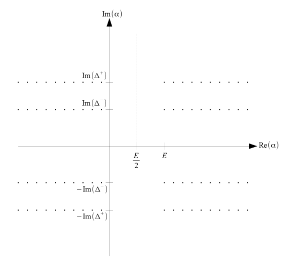
Figure 1: Integration path for the fusion of two non-degenerate states.

We now consider the case where one of the states in the OPE, say $\alpha_{2}$, is associated to a degenerate representation, i.e. $\alpha_{2}=-\vec{n}\cdot\vec{\omega}/2$ for a certain set of non-negative integers $n_{1},n_{2},n_{3}$. This OPE is computed via meromorphic analytical continuation as shown in Ponsot:2000mt , that is we set $\alpha_{2}=-\vec{n}\cdot\vec{\omega}/2+i\delta$ and consider the limit $\delta\rightarrow 0$. In this limit, due to the factor $S_{3}(2\alpha_{2})$ in the numerator of the 3-point functions, the OPE vanishes on the complex plane, except on the points where the denominator of the 3-point function becomes singular. As shown in Fig. 2, the integration path in (91) is deformed, and the integral receives contribution only from the discrete set of points where the denominator develop double poles, that are located at

$$\alpha=\alpha_{1}-\vec{s}\cdot\vec{\omega}/2\quad\quad\text{for any}\quad s_{k}\in\{-n_{k},-n_{k}+2,\ldots,n_{k}-2,n_{k}\}\,\quad\text{where}\quad k=1,2,3.$$ (98)

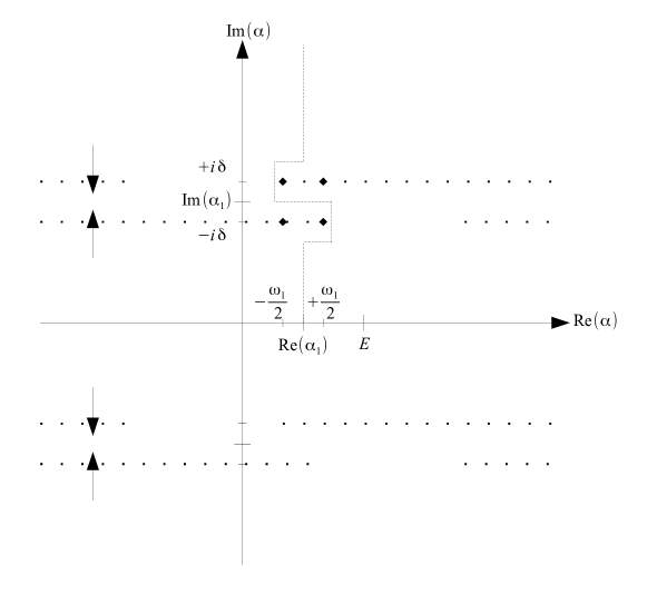
Figure 2: Pinching of the integration contour as the 3-point functions are continued to the degenerate values.

The result is computed by picking the residues at these poles, and shows that the OPE of a non-degenerate state with a degenerate state, include only a finite set of primaries, as in standard CFT. For instance, in the simplest case where we take $n=(0,0,1)$ (that is, $\alpha_{2}=-\omega_{3}/2$), there are only two contributing poles located at

$$\alpha=\alpha_{1}\pm\omega_{3}/2\,.$$ (99)

This produces the fusion rule

$$[\alpha]\times[-\frac{\omega_{3}}{2}]=[\alpha-\frac{\omega_{3}}{2}]+[\alpha+\frac{\omega_{3}}{2}]\,,$$ (100)

which is analogous to the well-know fusion rule between a level-2 degenerate state and a non-degenerate state in Liouville CFT.

From these degenerate fusion rules, we can conclude that the internal channel of a degenerate 4-point function includes only a discrete set of states. In particular, in the case where one of the four external states assumes the lowest degenerate momentum $-\omega_{3}/2$, the internal channel includes only 2 states. We have encountered this result already in section 2.3 in the gauge theory setup. Indeed, as we have already mentioned, the degeneration of 5d partition functions to 3d partition functions is the gauge theory realization of the degeneration limit of $q$-correlators, where the degeneration of the external state momentum in the $q$-correlator corresponds to an analytical continuation of the mass parameters in the gauge theory. In particular, in the gauge theory degeneration limit, the Coulomb branch integral reduces to the sum over the two points given in (50), that correspond to the momenta of the two internal states given in (99). Considering a generic degenerate state $\alpha_{2}=-\vec{n}\cdot\vec{\omega}/2$, the total number of contributing double poles is $(n_{1}+1)(n_{2}+1)(n_{3}+1)$ which yields the same number of states in the OPE. In the particular case of the 4-point correlator with a degenerate insertion $\alpha_{2}=-\vec{n}\cdot\vec{\omega}/2$, the $(n_{1}+1)(n_{2}+1)(n_{3}+1)$ internal states should correspond to the independent solutions of a certain difference operator. This is the $q$-CFT analogue of the higher degeneration of $S^{5}$ partition functions described in section 2.3.1.

4 Reflection coefficients

As we reviewed in the previous section, the two families of deformed Virasoro theories which we have been discussing, the $id$-CFT and $S$-CFT, were constructed in Nieri:2013yra by means of the bootstrap method. This approach does not rely on the Lagrangian formulation of the theory which in the present case is indeed not available and it is purely axiomatic since it uses the representation theory of the deformed Virasoro algebra and an ansatz for the way ${\cal V}ir_{q,t}$ blocks are paired to construct correlators.

However it would still be useful to develop a more physical or at least a geometrical (rather than purely algebraic) understanding of these theories. For this reason in this section we focus on reflection coefficients.

In Liouville field theory (LFT) the reflection coefficient can be defined in terms of 3-point functions, hence derived axiomatically from the bootstrap approach. However, it can also be obtained from a semiclassical analysis studying the reflection from the Liouville wall. In this sense the reflection coefficient bridges between the axiomatical and the semiclassical approach and appears to be an interesting object to study in the $q$-deformed cases. Furthermore, as we will see, reflection coefficients constructed from $id$-CFT and $S$-CFT 3-point functions are different, hence they are sensitive to the way ${\cal V}ir_{q,t}$ blocks are paired to construct correlators. Therefore we expect that the study of reflection coefficients will help us to put into perspective the relation between the two families of $q$-Virasoro systems and LFT.

4.1 Liouville Field Theory

In LFT the reflection coefficient is defined as the following ratio of DOZZ 3-point functions Zamolodchikov:1995aa

$$R_{L}(P)=\frac{C(Q_{0}-\alpha,\alpha_{2},\alpha_{1})}{C(\alpha,\alpha_{2},\alpha_{1})}\,,\quad P=i\alpha-iQ_{0}/2\,,$$ (101)

where $Q_{0}=b_{0}+1/b_{0}$ and $b_{0}$ is the Liouville coupling. Using the DOZZ formula for 3-point functions Dorn:1992at ; Dorn:1994xn ; Zamolodchikov:1995aa

$$C(\alpha_{3},\alpha_{2},\alpha_{1})=\frac{\Upsilon(2\alpha_{3})\Upsilon(2\alpha_{2})\Upsilon(2\alpha_{1})}{\Upsilon(\alpha_{1}+\alpha_{2}+\alpha_{3}-Q_{0})\Upsilon(-\alpha_{1}+\alpha_{2}+\alpha_{3})\Upsilon(\alpha_{1}-\alpha_{2}+\alpha_{3})\Upsilon(\alpha_{1}+\alpha_{2}-\alpha_{3})}\,,$$ (102)

one finds:

$$R_{L}(P)=\frac{\Upsilon(-2iP)}{\Upsilon(2iP)}=-\frac{\Gamma(2iPb_{0})\Gamma(2iP/b_{0})}{\Gamma(-2iPb_{0})\Gamma(-2iP/b_{0})}\,.$$ (103)

The reflection coefficient can be also obtained from a semiclassical analysis known an as the mini-superspace approximation Seiberg , where one ignores oscillator modes and focuses on the dynamics of the zero-mode $\phi_{0}$ of the Liouville field, governed by the Hamiltonian Zamolodchikov:1995aa

$$H_{0}=-\frac{1}{12}-\frac{1}{2}\frac{\partial^{2}}{\partial\phi_{0}^{2}}+2\pi\mu e^{2b_{0}\phi_{0}}.$$ (104)

The Schrödinger equation for the zero-mode of the Liouville field which scatters from an exponential barrier, since at $\phi_{0}\to-\infty$ the potential vanishes, has stationary asymptotic solutions of the form

$$\psi\sim e^{2iP\phi_{0}}+R(P)e^{-2iP\phi_{0}}\,.$$ (105)

Given that the eigenvalue problem

$$-\partial^{2}_{\phi_{0}}\psi_{P}+4\pi\mu e^{2b_{0}\phi_{0}}\psi_{P}=4P^{2}\psi_{P}$$ (106)

is solved by the modified Bessel function of the first kind, the reflection amplitude $R(P)$ can be easily extracted and reads

$$R(P)\sim\frac{\Gamma(2iP/b_{0})}{\Gamma(-2iP/b_{0})}.$$ (107)

This is a semi-classical result valid when $b_{0}\to 0$, indeed it captures only a part of the exact reflection coefficient (101). Therefore $R_{L}(P)$ can be considered the full quantum completion (i.e. including the non-perturbative $1/b_{0}$ contribution) of the reflection amplitude $R(P)$ computed from the 1st quantized Liouville theory.

There is also another (geometric) realization of the above problem, related to harmonic analysis on symmetric spaces. Often, 1d Schrödinger problems can be mapped to free motion of particles in curved spaces, where a potential-like term arises once the flat kinetic term is isolated from the Laplace-Beltrami operator. This is indeed the case for the Liouville eigenvalue problem (106) which appears in the study of the Laplace-Beltrami operator on the hyperboloid

$$\{(X_{0},X_{1},X_{2},X_{3})\in\mathbb{R}^{3,1}\Big{|}\;X_{0}^{2}-X_{1}^{2}-X_{2}^{2}-X_{3}^{2}=1\}\,.$$ (108)

Parameterising the hyperboloid (108) by horospherical coordinates $(x,r,\phi)$ as

$$X_{0}=\cosh\frac{x}{2}+\frac{r^{2}}{2}e^{-x/2};\quad X_{1}=-\sinh\frac{x}{2}-\frac{r^{2}}{2}e^{-x/2};\quad X_{2}=re^{-x/2}\cos\phi;\quad X_{3}=re^{-x/2}\sin\phi\,,$$ (109)

the Laplace-Beltrami operator defined by

$$\nabla^{2}=\frac{1}{\sqrt{{\rm det}~{}g}}\partial_{i}\sqrt{{\rm det}~{}g}~{}g^{ij}\partial_{j}\,,\qquad i=x,r,\phi\,,$$

with $g_{ij}=\partial_{i}\vec{X}\cdot\partial_{j}\vec{X}$ the induced metric, yields:

$$\nabla^{2}\Phi=\left(4\partial_{x}^{2}-4\partial_{x}+e^{x}\partial^{2}_{r}+\frac{e^{x}}{r}\partial_{r}+\frac{e^{x}}{r^{2}}\partial^{2}_{\phi}\right)\Phi\,.$$ (110)

Upon the reduction

$$\Phi(x,r,\phi)=\rho(r)e^{x/2}\psi(x)\,,\qquad\rho^{\prime\prime}+\rho^{\prime}/r=-4k\rho\,,$$

the Laplace-Beltrami operator becomes:

$$\nabla^{2}\Phi=\rho(r)e^{x/2}\left(4\partial^{2}_{x}\psi(x)-4ke^{x}\psi(x)-\psi(x)\right)\,,$$ (111)

corresponding indeed to the Hamiltonian $H_{0}$ given in (104). The free motion $-\nabla^{2}\Phi=\lambda^{2}\Phi$ is in turn translated into the Liouville eigenvalue equation (106)

$$-\partial^{2}_{x}\psi_{\lambda}(x)+ke^{x}\psi_{\lambda}(x)=\lambda^{2}\psi_{\lambda}(x)\,,$$ (112)

with asymptotic solutions of the form

$$\psi_{\lambda}(x)\sim c(\lambda)e^{i\lambda x}+c(-\lambda)e^{-i\lambda x}\quad\text{ as }\quad x\to-\infty\,.$$ (113)

The coefficients $c(\pm\lambda)$ are known in this context as Harish-Chandra $c$-functions, which for the hyperboloid (108) are given by:

$$c(\lambda)=\frac{1}{\Gamma(1+2i\lambda)}\,,$$ (114)

yielding

$$\frac{c(-\lambda)}{c(\lambda)}=-\frac{\Gamma(2i\lambda)}{\Gamma(-2i\lambda)}\,,$$ (115)

which, with the identification $P/b_{0}=\lambda$, corresponds to the semiclassical result (107).

The hyperboloid (108) is isomorphic to the Lobachevsky space $SO_{0}(1,3)/SO(3)\simeq SL(2,\mathbb{C})/SU(2)$. In the study of group manifolds the Laplace-Beltrami operator appears from the analysis of the quadratic Casimirs. In particular, horospheric coordinates can be introduced for any hyperbolic symmetric space, reflecting the Iwasawa decomposition of the group manifold. The plane wave asymptotic behaviour of the eigenfunctions of the reduced Laplace-Beltrami operator is then governed by the Harish-Chandra $c$-functions as in the case of the hyperboloid. In fact, $c$-functions of any classical symmetric space can be expressed as a product of Gamma functions (Gindikin-Karpelevich formula, see for instance Helgason , cf. HelgasonI ). In horospherical coordinates (e.g. GerasimovKharchevMarshakovMironovMorozovOlshanetsky ), one has

$$c(\lambda)=\prod_{\alpha\in\Delta^{+}}\frac{1}{\Gamma(l+\lambda\cdot\alpha)}\,,$$ (116)

where $\lambda$ is a spectral parameter for the eigenvalues of the Laplacian, $\Delta^{+}$ denotes the positive roots of the Lie algebra of the group modelling the symmetric space, and $l=1$ for finite dimensional Lie algebras or $l=1/2$ for the affine version thereof. The reflection coefficient of the associated quantum mechanical system can be computed as the ratio $c(-P)/c(P)$, where the momentum $P$ is parameterised by $\lambda\cdot\alpha$.

As we already observed, the semiclassical reflection coefficient $R(P)$ (115) or (107) reproduces only part of the exact LFT reflection coefficient $R_{L}(P)$ (103). There is however a group theoretic method GerasimovKharchevMarshakovMironovMorozovOlshanetsky to obtain the non-perturbative or 2nd quantized completion of the LFT reflection coefficient. To this end, one considers the extension of the root system, which in the $\mathfrak{sl}(2)$ case contains only one positive root $\alpha_{1}$, by the affine root $\alpha_{0}$ so that upon affinization $\mathfrak{sl}(2)\rightarrow\widehat{\mathfrak{sl}}(2)$ the positive roots become:

$$\alpha_{0}+n\delta,\quad n\delta,\quad\alpha_{1}+n\delta,\quad\delta\equiv\alpha_{0}+\alpha_{1},\quad n\in\mathbb{Z}^{+}_{0}\,.$$ (117)

The Harish-Chandra function is then given by the product (116) over the extended root system and, choosing the parameterization

$$\lambda\cdot\delta=\tau,\quad\lambda\cdot\alpha_{1}=2iP/b_{0}-1/2,\quad\lambda\cdot\alpha_{0}=\tau-2iP_{0}/b_{0}+1/2\,,$$ (118)

becomes

$$\displaystyle c(P)^{-1} \equiv \prod_{n\geq 0}\Gamma(1/2+\lambda\cdot(\alpha_{1}+n\delta))\prod_{n\geq 0}\Gamma(1/2+\lambda\cdot(\alpha_{0}+n\delta))\prod_{n\geq 1}\Gamma(1/2+\lambda\cdot n\delta)$$ (119)

$$= \Gamma(2iP/b_{0})\prod_{n\geq 1}\Gamma(2iP/b_{0}+n\tau)\Gamma(1-2iP/b_{0}+n\tau)\Gamma(1/2+n\tau)\,.$$

It is easy to check that the $n=0$ factor reproduces the non-affinized/semiclassical result while the ratio of $c$-functions

$$\displaystyle\frac{c(-P)}{c(P)} = \frac{\Gamma(2iP/b_{0})}{\Gamma(-2iP/b_{0})}\prod_{n\geq 1}\frac{\Gamma(2iP/b_{0}+n\tau)\Gamma(1-2iP/b_{0}+n\tau)}{\Gamma(-2iP/b_{0}+n\tau)\Gamma(1+2iP/b_{0}+n\tau)}$$ (120)

$$\sim -\frac{\Gamma(2iP/b_{0})}{\Gamma(-2iP/b_{0})}\frac{\Gamma(2iP/b_{0}\tau)}{\Gamma(-2iP/b_{0}\tau)}\,,$$

upon identifying $\tau=1/b_{0}^{2}$, reproduces the exact LFT reflection coefficient $R_{L}$ (103).

The above discussion suggests to regard the affinization as a prescription for an effective 2nd quantization. As we are about to see, this prescription works remarkably well for our $q$-Virasoro systems.

4.2 $id$-CFT

We begin by computing the $id$-CFT reflection coefficient in terms of the $id$-pairing 3-point functions given in (83):

$$R_{id}(P)=\frac{C_{id}(Q_{0}-\alpha,\alpha_{2},\alpha_{1})}{C_{id}(\alpha,\alpha_{2},\alpha_{1})}=\frac{\Upsilon^{\beta}(-2iP)}{\Upsilon^{\beta}(2iP)}\,,\qquad P=i\alpha-iQ_{0}/2\,,$$ (121)

which can be rewritten in terms of the $q$-deformed $\Gamma$ function:

$$\Gamma_{q}(x):=\frac{(q;q)}{(q^{x};q)}(1-q)^{1-x}\,,$$ (122)

as

$$R_{id}(P)\sim\frac{(1-q)^{4iPb_{0}}}{(1-t)^{-4iP/b_{0}}}\frac{1-q^{2iPb_{0}}}{1-t^{-2iP/b_{0}}}\times\frac{\Gamma_{q}\left(2iPb_{0}\right)\Gamma_{t}\left(2iP/b_{0}\right)}{\Gamma_{q}\left(-2iPb_{0}\right)\Gamma_{t}\left(-2iP/b_{0}\right)}\,,$$ (123)

with $q=e^{\beta/b_{0}}$ and $t=e^{\beta b_{0}}$.

The above expression suggests that in this case the 1st quantized reflection coefficient should be captured by a $c$-function expressed in terms of products over the $\mathfrak{sl}(2)$ root system of $q$-deformed (with deformation parameter $t$) Gamma functions

$$c(\lambda)=\frac{1}{\Gamma_{t}(l+\lambda\cdot\alpha)}\,,$$ (124)

while the affinization prescription should allow to recover the non-perturbative reflection coefficient (123). Indeed proceeding as in the LFT case (117), (118), we obtain

$$c(P)^{-1}=\prod_{n\geq 0}\Gamma_{t}(2iP/b_{0}+n\tau)\Gamma_{t}(1-2iP/b_{0}+(n+1)\tau)\prod_{n\geq 1}\Gamma_{t}(1/2+n\tau)\,,$$ (125)

which, after dropping $P$-independent factors and defining $q=t^{\tau}$, becomes

$$c(P)\sim(t^{2iP/b_{0}};q,t)(qt^{1-2iP/b_{0}};q,t)=\frac{(t^{2iP/b_{0}};q,t)(t^{1-2iP/b_{0}};q,t)}{(t^{1-2iP/b_{0}};t)}\,.$$ (126)

It is immediate to verify that the ratio of $c$-functions

$$\displaystyle\frac{c(-P)}{c(P)} = \frac{(1-q)^{4iPb_{0}}}{(1-t)^{-4iP/b_{0}}}\frac{1-q^{2iPb_{0}}}{1-t^{-2iP/b_{0}}}\frac{\Gamma_{q}\left(2iPb_{0}\right)\Gamma_{t}\left(2iP/b_{0}\right)}{\Gamma_{q}\left(-2iPb_{0}\right)\Gamma_{t}\left(-2iP/b_{0}\right)},$$ (127)

reproduces $R_{id}$ once we set $\tau=1/b_{0}^{2}$. Since $\Gamma_{q}\to\Gamma$ as $q\to 1$, we can also check that, as expected, in the $\beta\to 0$ limit the $id$-CFT reflection coefficient $R_{id}$ reduces to the LFT one $R_{L}$.

The $c$-function (124), suggested by the naive $q$-deformation of the Liouville case, actually appears in OlshanetskyRogov (see also FreundZabrodinI ; FreundZabrodinII ; FreundZabrodinIV ) ) as the genuine $c$-function in the quantum Lobachevsky space. In that case the relevant quantum group is $U_{q}(\mathfrak{sl}(2))$, and the quadratic Casimir can be studied introducing horospherical coordinates in the quantum space. The eigenvalue problem and asymptotic analysis then leads exactly to (124). In particular the eigenvalue problem from which the $c$-function is derived is a discretized version of the Schrödinger-Liouville equation (112).

Finally, let us explain why we can expect the affinization procedure to work also in the case of a quantum affine algebra $U_{q}(\widehat{\mathfrak{g}})$, with $\mathfrak{g}$ a simple Lie algebra. In fact, once we assume a specific form of the $c$-function for the non-affine part $\mathfrak{g}$, we can rely on the fact that the root structure is the same for $U_{q}(\widehat{\mathfrak{g}})$ as it is for the undeformed affine case $\widehat{\mathfrak{g}}$ LevendorskiiSoibelmanStukopin . This is made particularly evident in what is known as Drinfeld’s second realization Drinfeld of quantum affine algebras. In this realization, to each of the infinite roots (117) is associated a particular generator labelled by the integer level $n$. Roots are divided into positive and negative, and naturally ordered according to increasing or decreasing $n$. The specification of the algebra is then completed by assigning a set of relations between the generators at the various levels.

4.3 $S$-CFT

The reflection coefficient constructed in terms of the $S$-CFT 3-point functions (82) is given by:

$$R_{S}(P)=\frac{C_{S}(E-\alpha,\alpha_{2},\alpha_{1})}{C_{S}(\alpha,\alpha_{2},\alpha_{1})}=\frac{S_{3}(-2iP|\vec{\omega})}{S_{3}(2iP|\vec{\omega})}\,,\quad P=i\alpha-iE/2\,.$$ (128)

In this case if we take a $c$-function given in terms of Barnes double Gamma functions

$$c(P)=\frac{1}{\Gamma_{2}(2iP/\kappa|e_{1},e_{2})}\,,\quad e_{1}+e_{2}=1\,,$$ (129)

while keeping the $\mathfrak{sl}(2)$ root system, and apply the affinization prescription we obtain

$$\displaystyle c(P)^{-1} = \prod_{n\geq 0}\Gamma_{2}(2iP/\kappa+n\tau|e_{1},e_{2})\Gamma_{2}(1-2iP/\kappa+(n+1)\tau|e_{1},e_{2})\prod_{n\geq 1}\Gamma_{2}(1/2+n\tau|e_{1},e_{2})$$

$$\sim\Gamma_{3}(2iP/\kappa|e_{1},e_{2},\tau)\Gamma_{3}(e_{1}+e_{2}+\tau-2iP/\kappa|e_{1},e_{2},\tau)=S_{3}(2iP/\kappa|e_{1},e_{2},\tau)^{-1}\,.$$

Finally, using $S_{3}(\kappa X|\kappa\vec{\omega})=S_{3}(X|\vec{\omega})$, we get

$$c(P)=S_{3}(2iP|\vec{\omega})\,,\quad\vec{\omega}=\kappa(e_{1},e_{2},\tau)\,,$$ (131)

from which it follows that the ratio $c(-P)/c(P)$ reproduces the exact reflection coefficient (128).

Notice that the Barnes $\Gamma_{2}$ function appears already in the affinized version of the Liouville $c$-function given in eq. (119) which indeed can be rewritten as

$$c(P)^{-1}\sim\Gamma_{2}(2iP|b_{0},b_{0}^{-1})\Gamma_{2}(Q_{0}-2iP|b_{0},b_{0}^{-1})\,,$$ (132)

so in a sense we may regard $R_{S}$ as arising from a 2nd affinization, or multi-loop algebra of $\mathfrak{sl}(2)$. Even if we are not aware of an explicit way to construct a space whose $c$-function is given by $\Gamma_{2}$ functions, it has been strongly motivated for example in FreundZabrodinII that such generalised $c$-functions should naturally be associated to such a construction, and to general families of integrable systems, whose S-matrix building blocks are indeed $\Gamma_{n}$ functions or deformations thereof (as we saw in the $id$-CFT) (see also e.g. Ruijsenaars ).

Before ending this section, let us observe that the reflection coefficients $R_{id}$ and $R_{S}$ satisfy the unitary condition $R_{id,S}(P)R_{id,S}(-P)=1$ by construction, and have zeros and poles determined by the factors $\Gamma_{q}$ and $\Gamma_{3}$ respectively. Moreover, we saw the Lie algebra $\mathfrak{sl}(2)$ played a prominent role in the study of the reflection coefficients through $c$-functions. As we are going to show in the next section, all these elements are of fundamental importance in integrable systems, and it is therefore natural to ask which known models feature the same structures we have just seen.

5 S-matrices

In the previous sections we have shown how it is possible to reproduce the reflection coefficients via an affinization procedure starting from putative Harish-Chandra $c$-functions OlshanetskyPerelomov ; FreundZabrodinIV (see also FaddeevH , comments following formula (217)). In this section we will connect these coefficients to known scattering matrices of integrable spin-chains and (related) integrable quantum field theories. Typically, the S-matrices are built by taking the ratio of the two Jost functions $J(u)$ with opposite arguments, as they appear in the plane-wave asymptotics of the scattering wave function:

$$\psi(x)\sim J(-u)e^{ipx}+J(u)e^{-ipx},\qquad x\to-\infty,\qquad S(u)=\frac{J(u)}{J(-u)},$$ (133)

with $p$ the momentum of the particle and $u$ the corresponding rapidity (for massive relativistic particles, $E=m\,\mbox{cosh}u$ and $p=m\,\mbox{sinh}u$).

We will find a relationship between known S-matrices/Jost functions computed in the literature and the $c$-functions we have been using, before the affinization takes place. The affinization

$$\mathfrak{sl}(2)\,\longrightarrow\,\widehat{\mathfrak{sl}}(2)$$ (134)

produces then the final expression for the reflection coefficients.

The starting point will be the S-matrix for two excitations of the XYZ spin-chain FaddeevTakhtadjan . The Hamiltonian for the XYZ chain reads

$$H=-\frac{1}{4}\sum_{n=1}^{N}\,\big{(}J_{x}\,\sigma_{n}^{x}\,\sigma_{n+1}^{x}+J_{y}\,\sigma_{n}^{y}\,\sigma_{n+1}^{y}+J_{z}\,\sigma_{n}^{z}\,\sigma_{n+1}^{z}\big{)},$$ (135)

where the sum is over all the sites of a chain of $N$ sites, and the spin at each site is $\frac{1}{2}$. We consider definite $z$-component of the spin, with the operators $\sigma_{n}^{i}$ being the Pauli matrices at site $n$.

The connection with the integrable 8-vertex model BaxterP is obtained by imposing the following parameterization in terms of Jacobi elliptic functions:

$$J_{x}=J\,\big{[}\mbox{cn}^{2}(\lambda,k^{\prime})+k\,\mbox{sn}^{2}(\lambda,k^{\prime})\big{]},\qquad J_{y}=J\,\big{[}\mbox{cn}^{2}(\lambda,k^{\prime})-k\,\mbox{sn}^{2}(\lambda,k^{\prime})\big{]}$$

$$J_{z}=-J\,\mbox{dn}(\lambda,k^{\prime}),\qquad\qquad k^{\prime}\equiv\sqrt{1-k^{2}},$$ (136)

where we will assume $J>0$, and the modulus $k$, the complementary modulus $k^{\prime}$ and the argument $\lambda$ to be a priori complex. In this fashion, the Hamiltonian (135) can be directly obtained (apart from an overall factor and a constant shift) from the transfer matrix of the 8-vertex model by taking its logarithmic derivative Baxter , in the spirit of the quantum inverse scattering method (cf. also Faddeev and appendix C).

One starts focusing on a particular region of the parameter space in the Hamiltonian (135), corresponding to the so-called principal regime

$$|J_{y}|\leq J_{x}\leq-J_{z}.$$ (137)

Any other region of the parameter space can be reached starting from (137) and performing suitable transformations Baxter . In this regime, let us recast the Hamiltonian in the following form:

$$H=-\frac{J_{x}}{4}\sum_{n=1}^{N}\,\big{(}\sigma_{n}^{x}\,\sigma_{n+1}^{x}+\Gamma\,\sigma_{n}^{y}\,\sigma_{n+1}^{y}-\Delta\,\sigma_{n}^{z}\,\sigma_{n+1}^{z}\big{)},$$

$$\Gamma\equiv\frac{J_{y}}{J_{x}},\qquad\Delta=-\frac{J_{z}}{J_{x}},\qquad J_{x}\geq 0,\qquad\Delta\geq 1.$$ (138)

One can see from $J_{x}\geq 0$ and $\Delta\geq 1$ that the chain is in an antiferromagnetic region, where the alignment of spins along the $z$-axis is energetically disfavoured. The ground state is a Dirac sea of filled levels over the false vacuum (which is the ferromagnetic one with all spins aligned), and the excitations are holes in the sea. These excitations scatter with a well defined S-matrix, which can in principle be obtained using the method of Korepin Korepin . In FreundZabrodinIV , the corresponding Jost function is written in terms of parameters $\gamma$ and $\tau$ as an infinite product of $\Gamma_{q}$ functions with shifted arguments, specifically

$$J(u)\,=\,\prod_{m=0}^{\infty}\,\frac{\Gamma_{q}(iu+rm)\Gamma_{q}(iu+rm+r+1)}{\Gamma_{q}(iu+rm+\frac{1}{2})\Gamma_{q}(iu+rm+r+\frac{1}{2})},$$ (139)

where

$$q\,=\,e^{-4\gamma},\qquad r\,=\,-\frac{i\pi\tau}{2\gamma},$$ (140)

$u$ being a spectral parameter equal to the difference of the incoming particle rapidities $u=u_{1}-u_{2}$, and we should set $\tau=\frac{i}{2}\frac{K^{\prime}}{K}$, where $K$ and $K^{\prime}$ (called, respectively, $I$ and $I^{\prime}$ in BaxterBook ) are the complete elliptic integrals of the first kind

$$K=\int_{0}^{\frac{\pi}{2}}\frac{dt}{\sqrt{1-k^{2}\sin^{2}t}},\qquad K^{\prime}=\int_{0}^{\frac{\pi}{2}}\frac{dt}{\sqrt{1-k^{\prime 2}\sin^{2}t}},\qquad k^{\prime\,2}=1-k^{2}.$$

Our two reflection coefficients corresponding, respectively, to the $id$- and to the $S$-pairing, as obtained in the previous sections, can be related to different limits of the above Jost function before the affinization procedure.

• Limit 1. Reproducing the special functions of the $id$-pairing

  Following CauxKonnoSorrellWeston , by sending $k\to 0$ with $\lambda$ fixed and real in (5) one obtains the following limit:

  $$J_{x}\to J\,\mbox{sech}^{2}\lambda\geq 0,\qquad J_{y}\to J\,\mbox{sech}^{2}\lambda,\qquad J_{z}\to-J\,\mbox{sech}\lambda,$$ (141)

  therefore the Hamiltonian reduces to

  $$H=-\frac{J}{4}\mbox{sech}^{2}\lambda\,\sum_{n=1}^{N}\,\big{(}\sigma_{n}^{x}\,\sigma_{n+1}^{x}+\,\sigma_{n}^{y}\,\sigma_{n+1}^{y}-\mbox{cosh}\lambda\,\sigma_{n}^{z}\,\sigma_{n+1}^{z}\big{)}.$$ (142)

  One can see that $\Gamma\to 1$ and $\Delta\to\mbox{cosh}\lambda\geq 1$ for real $\lambda$. This means that the limiting chain is an XXZ spin-chain in its antiferromagnetic regime. Moreover, the regime $\Delta\geq 1$ is massive, meaning that the spectrum of excitations (holes in the Dirac sea) has a mass gap.

  The limit $k\to 0$ corresponds to sending $\tau\to i\infty$, since $K^{\prime}\to+\infty$ and $K\to\frac{\pi}{2}$. If one performs this limit in the expression (139) FreundZabrodinIV , only part of the $k=0$ term survives the limit and one obtains FreundZabrodinI ; FreundZabrodin (up to an overall factor) the Jost function for the scattering of a kink and an anti-kink in the antiferromagnetic spin-$\frac{1}{2}$ XXZ spin-chain, in terms of a ratio of two $\Gamma_{q}$ functions

  $$J(u)\,\to\,\frac{\Gamma_{q}(iu)}{\Gamma_{q}(iu+\frac{1}{2})}.$$ (143)

  The same scattering factor is also obtained (in a slightly different parameterization) in DaviesFodaJimboMiwaNakayashiki , as a multiplier of the R-matrix for a $U_{q}(\widehat{\mathfrak{sl}}(2))$ doublet of excitations of the antiferromagnetic massive XXZ spin-chain.

  The same structure features in our $id$-pairing reflection coefficient. As we recalled in section 4.2, the authors of OlshanetskyRogov derive the Harish-Chandra function (143) by studying the quantum Lobachevsky space and already point out the connection to the XXZ quantum spin-chain via (143).

• Limit 2. Reproducing the special functions of the $S$-pairing

  The second limit considered in CauxKonnoSorrellWeston is composed of two operations. Firstly, one performs a transformation that maps the parameters of the Hamiltonian (135) as follows:

  $$J_{x}\to J_{x}^{\prime}=-J_{z},\qquad J_{y}\to J_{y}^{\prime}=J_{x},\qquad J_{z}\to J_{z}^{\prime}=-J_{y}$$ (144)

  The above transformation maps the principal regime of the Hamiltonian (135) to its disordered regime:

  $$|J_{z}^{\prime}|\leq J_{y}^{\prime}\leq J_{x}^{\prime}.$$

  Secondly, by sending now $k\to 1$ with $\lambda$ fixed in (5) one obtains the following limit:

  $$J_{x}^{\prime}=-J_{z}\to J,\qquad J_{y}^{\prime}=J_{x}\to J,\qquad J_{z}^{\prime}=-J_{y}\to-J\cos 2\lambda,$$ (145)

  therefore the Hamiltonian reduces to

  $$H=-\frac{J}{4}\,\sum_{n=1}^{N}\,\big{(}\sigma_{n}^{x}\,\sigma_{n+1}^{x}+\,\sigma_{n}^{y}\,\sigma_{n+1}^{y}-\cos 2\lambda\,\,\sigma_{n}^{z}\,\sigma_{n+1}^{z}\big{)}.$$ (146)

  One can see that $\Gamma\to 1$ and $|\Delta|\to|\cos 2\lambda|\geq 1$ for real $\lambda$. This means that the limiting chain is an XXZ spin-chain in its disordered regime. The regime $|\Delta|\leq 1$ is massless, meaning that the spectrum of excitations (holes in the Dirac sea), called “spinons” in this case (with spin equal to $\frac{1}{2}$), has no mass gap. For $\Delta=0$ the excitations are described by a theory of free fermions.

  The limit $k\to 1$ corresponds to sending $\tau\to 0$, since $K\to+\infty$ and $K^{\prime}\to\frac{\pi}{2}$ in this case. If one performs this limit in the expression (139), as pointed out in FreundZabrodinIV , namely one first sends $q\to 1$ with $r$ fixed, one obtains an infinite product of ordinary $\Gamma$ functions:

  $$J(u)\,\to\,\prod_{m=0}^{\infty}\,\frac{\Gamma(iu+rm)\Gamma(iu+rm+r+1)}{\Gamma(iu+rm+\frac{1}{2})\Gamma(iu+rm+r+\frac{1}{2})}.$$ (147)

  The corresponding S-matrix is calculated according to (133). One can rewrite the resulting infinite product of $\Gamma$ functions as

  $$S = \frac{J(u)}{J(-u)}\,\to$$ (148)

  $$\to \prod_{n=0}^{\infty}\frac{\Gamma\Big{(}\frac{1}{2}+n\,\Sigma-\frac{v}{2}\Big{)}}{\Gamma\Big{(}\frac{1}{2}+n\,\Sigma+\frac{v}{2}\Big{)}}\frac{\Gamma\Big{(}1+n\,\Sigma+\frac{v}{2}\Big{)}}{\Gamma\Big{(}1+n\,\Sigma-\frac{v}{2}\Big{)}}\frac{\Gamma\Big{(}(n+1)\,\Sigma+\frac{v}{2}\Big{)}}{\Gamma\Big{(}(n+1)\,\Sigma-\frac{v}{2}\Big{)}}\frac{\Gamma\Big{(}\frac{1}{2}+(n+1)\,\Sigma-\frac{v}{2}\Big{)}}{\Gamma\Big{(}\frac{1}{2}+(n+1)\,\Sigma+\frac{v}{2}\Big{)}}$$

  $$\sim \frac{\Gamma_{2}\Big{(}\frac{1-v}{2}|1,\Sigma\Big{)}\Gamma_{2}\Big{(}\frac{1+v}{2}|1,\Sigma\Big{)}\Gamma_{2}\Big{(}\frac{v}{2}+\Sigma|1,\Sigma\Big{)}\Gamma_{2}\Big{(}\frac{1-v}{2}+\Sigma|1,\Sigma\Big{)}}{\Gamma_{2}\Big{(}\frac{1+v}{2}|1,\Sigma\Big{)}\Gamma_{2}\Big{(}\frac{1-v}{2}|1,\Sigma\Big{)}\Gamma_{2}\Big{(}\Sigma-\frac{v}{2}|1,\Sigma\Big{)}\Gamma_{2}\Big{(}\frac{1+v}{2}+\Sigma|1,\Sigma\Big{)}\,},$$

  where $\Sigma=r$ and $v=2iu$. The $\Gamma_{2}$ function is the same function we saw playing a r$\hat{\mbox{o}}$le in the $S$-pairing calculation, cf. section 4.3. In terms of Jost functions, we have

  $$J(u)\to\frac{\Gamma_{2}\Big{(}\frac{1+v}{2}|1,\Sigma\Big{)}\Gamma_{2}\Big{(}\frac{v}{2}+\Sigma|1,\Sigma\Big{)}}{\Gamma_{2}\Big{(}\frac{1+v}{2}|1,\Sigma\Big{)}\Gamma_{2}\Big{(}\frac{1+v}{2}+\Sigma|1,\Sigma\Big{)}},$$ (149)

  which is the analogue of (143). The above S-matrix is often found re-expressed using an integral representation (see for instance KirillovReshetikhin ; DoikouNepomechie ):

  $$S=\exp\bigg{[}\int_{0}^{\infty}\frac{\sinh(vs)\,\sinh\big{[}s(\Sigma-\frac{1}{2})\big{]}}{s\,\cosh(\frac{s}{2})\sinh(\Sigma\,s)}\,ds\,\bigg{]}.$$ (150)

  The S-matrix (148) has also been obtained directly in the spin-chain setting for a spin-zero two-particle state of the spin-$\frac{1}{2}$ XXZ chain in its massless regime BabujianTsvelik ; KirillovReshetikhin ; DoikouNepomechie .

• Limit 3. Alternative route to the special functions of the $S$-pairing

  By introducing the variable

  $$\delta\equiv\frac{\lambda}{K},$$ (151)

  one can see, for instance, that the Limit 2 above can be equivalently obtained as $\delta\to 0$. Alternatively, CauxKonnoSorrellWeston reports a limit where a suitably introduced lattice spacing $\epsilon$ scales to zero alongside with the parameter $\delta$ such that

  $$\delta\to 0,\qquad\epsilon\to 0,\qquad 2\,\frac{e^{-\frac{\pi}{\delta}}}{\epsilon}\to M\,\mbox{finite}.$$

  The number of spin-chain sites is also taken to be infinite, hence, in this limit, the discrete chain tends to a continuum model, which turns out to be the Sine-Gordon theory LukyanovTerras . The parameter $M$ plays the role of the mass entering the particle dispersion relation in the continuum model. The Sine-Gordon spectrum is massive and consists of a soliton, an anti-soliton and a tower of corresponding bound states (the so-called breathers).

  Since the Sine-Gordon limit still involves sending $\delta\to 0$, we expect a similar type of S-matrix as in the case of Limit 2. In fact, the limiting expression in terms of an infinite product of gamma functions famously reproduces (apart from overall factors) the Jost function for the (anti-)soliton and (anti-)soliton scattering in the Sine-Gordon theory ZamolodchikovZamolodchikov , or, equivalently, for the excitations of the massive Thirring model Korepin , Coleman . The S-matrix is given by (148), with the parameter $\Sigma$ now related to the Sine-Gordon coupling constant.

  The XXZ chain in its disordered regime has been connected to a lattice regularization of Sine-Gordon and Liouville theory in FaddeevTirkkonen . A similar relationship between the modular XXZ chain and the lattice Sinh-Gordon theory has been explored in BytskoTeschner .

We remark that in gaddegukovputrovwalls it was shown that 3d $\mathcal{N}=2$ solid tori partition functions satisfy the Baxter equation for the $\mathfrak{sl}(2)$ XXZ spin-chain. In appendix E we offer another derivation of this relation showing that the hypergeometric difference equation satisfied by the 3d holomorphic blocks ${\cal B}^{3d}_{\alpha}$ can be mapped to the Baxter equation for the $\mathfrak{sl}(2)$ XXZ spin-chain.

For the sake of completeness, we recall that the very same S-matrix (148) also features in the scattering of two spin-$\frac{1}{2}$ spin-wave excitations propagating on the antiferromagnetic XXX spin-chain with arbitrary spin $\Sigma$ representation at each site Takhtajan ; Reshetikhin (the spin $\Sigma$ entering the formula in a similar way as the coupling constant does in the case of the Sine-Gordon model). Namely, for a spectral parameter $w$ and a singlet-triplet system of excitations,

$$S\,=\,S_{\frac{1}{2}}\,\cdot\frac{\sinh\big{(}\frac{\pi}{4\Sigma}(w-i)\big{)}}{\sinh\big{(}\frac{\pi}{4\Sigma}(w+i)\big{)}}\,\,\exp\bigg{[}-i\int_{0}^{\infty}\frac{\sin(ws)\,\sinh\big{[}s(\Sigma-\frac{1}{2})\big{]}}{s\,\cosh(\frac{s}{2})\sinh(\Sigma\,s)}\,ds\,\bigg{]},$$ (152)

where $S_{\frac{1}{2}}$ is the S-matrix for spin-$\frac{1}{2}$ particles, related to the central extension of the $\mathfrak{sl}(2)$ Yangian double KhoroshkinLebedevPakuliak :

$$S_{\frac{1}{2}}\,=\,\frac{\Gamma(-i\frac{w}{2})\Gamma(\frac{1}{2}+i\frac{w}{2})}{\Gamma(i\frac{w}{2})\Gamma(\frac{1}{2}-i\frac{w}{2})}\,\cdot\,\frac{w-i\,{\mathbb{P}}}{w-i},\qquad{\mathbb{P}}=\mbox{permutation in $\mathbb{C}^{2}\otimes\mathbb{C}^{2}$}.$$ (153)

Let us finally point out that the S-matrix (153) appears also in connection with the massless limit of the $\mathfrak{su}(2)$ Thirring model ZamolodchikovZamolodchikovI .

If one proceeds one steps “downwards”, one can take the limit $q\to 1$ of (143) and obtain a Jost function written in terms of a ratio of ordinary Gamma functions. This reproduces FreundZabrodinI the scattering of two spin-$\frac{1}{2}$ spin-wave (kink) excitations of the XXX spin-$\frac{1}{2}$ spin-chain FaddeevTakhtajanI ; FaddeevTakhtajan , i.e. the triplet part of formula (153). This limit corresponds to sending $\gamma\sim\lambda\to 0$ (see appendix D, where $K^{\prime}_{l}$ has been sent to a constant in Limit 1), from which we see that the Hamiltonian reduces to the one of the antiferromagnetic isotropic spin-chain, for which one can then use the equivalence of spectra $H(\Delta)\leftrightarrow-H(-\Delta)$ Samaj . This in turn produces a similar structure as the mini-superspace Liouville reflection coefficient, which has been obtained in OlshanetskyRogov by studying the ordinary Lobachevsky space (see also GerasimovMarshakovOlshanetskyShatashvili ; GerasimovMarshakovMorozovOlshanetskyShatashvili ). This is in agreement with the fact that in the $q\to 1$ limit the $id$-CFT reduces to Liouville theory Nieri:2013yra .

We remark that the semiclassical reflection coefficient of the Liouville theory contains only part of the gamma functions present in formula (153).

This is related to the fact that the reflection coefficient, in the semiclassical limit $b_{0}\to 0$, can also be interpreted as the S-matrix for the scattering of a quantum mechanical particle against a static potential (mini-superspace approximation Zamolodchikov:1995aa ; Seiberg ). In one case the potential is given by the Liouville one, in the other case it is given by the (Calogero-Moser-Sutherland type) potential $\propto\sinh^{-2}x$ OlshanetskyPerelomov (see also Inozemtsev ).

The other reflection coefficients we have derived in the previous section, i.e. for the $id$- and $S$-pairing, call for analogous considerations. For the $id$-pairing, producing the Harish-Chandra functions of OlshanetskyRogov , and similarly for the $S$-pairing, we again retain a reduced number of the special functions as compared to what characterizes the S-matrices of the integrable (spin-chain) models we discuss in this section.

Let us finally point out once more that in this whole discussion it is understood that affinization has yet to be performed. It would be very interesting to study what spin-chain picture might arise, if any, when the affinization takes place.

Appendix A Special functions

In this appendix we describe few of the special functions and identities used in the main text.

A.1 Bernoulli polynomials

Throughtout this appendix let us denote by

$$\vec{\omega}:=(\omega_{1},\ldots,\omega_{r})\in\mathbb{C}^{r}$$ (154)

a vector of $r$ parameters. The multiple Bernoulli polynomials $B_{rr}(z|\vec{\omega})$ up to cubic order are defined by naru

$$\displaystyle B_{11}(z|\vec{\omega})= \frac{z}{\omega_{1}}-\frac{1}{2}$$

$$B_{22}(z|\vec{\omega})= \frac{z^{2}}{\omega_{1}\omega_{2}}-\frac{\omega_{1}+\omega_{2}}{\omega_{1}\omega_{2}}z+\frac{\omega_{1}^{2}+\omega_{2}^{2}+3\omega_{1}\omega_{2}}{\omega_{1}\omega_{2}}$$

$$B_{33}(z|\vec{\omega})= \frac{z^{3}}{\omega_{1}\omega_{2}\omega_{3}}-\frac{3\,(\omega_{1}+\omega_{2}+\omega_{3})}{2\,\omega_{1}\omega_{2}\omega_{3}}z^{2}+\frac{\omega_{1}^{2}+\omega_{2}^{2}+\omega_{3}^{2}+3(\omega_{1}\omega_{2}+\omega_{2}\omega_{3}+\omega_{3}\omega_{1})}{2\,\omega_{1}\omega_{2}\omega_{3}}z$$ (155)

$$-\frac{(\omega_{1}+\omega_{2}+\omega_{3})(\omega_{1}\omega_{2}+\omega_{2}\omega_{3}+\omega_{3}\omega_{1})}{4\,\omega_{1}\omega_{2}\omega_{3}}\,.$$

If not stated otherwise, we will use the shorthand notation $B_{rr}(z):=B_{rr}(z|\vec{\omega})$.

A.2 Multiple Gamma and Sine functions

The Barnes $r$-Gamma function $\Gamma_{r}(z|\vec{\omega})$ can be defined as the $\zeta$-regularized infinite product naru

$$\Gamma_{r}(z|\vec{\omega})\sim\prod_{\vec{n}\in\mathbb{Z}^{+}_{0}}\frac{1}{\left(z+\vec{\omega}\cdot\vec{n}\right)}.$$ (156)

When there is no possibility of confusion, we will simply set $\Gamma_{r}(z):=\Gamma_{r}(z|\vec{\omega})$.

The $r$-Sine function is defined according to naru

$$S_{r}(z|\vec{\omega})=\frac{\Gamma_{r}(E_{r}-z)^{(-1)^{r}}}{\Gamma_{r}(z)}$$ (157)

where we defined $E_{r}:=\sum_{i}\omega_{i}$. We will also denote $S_{r}(z):=S_{r}(z|\vec{\omega})$ when there is no confusion. Also, introducing the multiple $q$-shifted factorial

$$\left(z;q_{1},\ldots q_{r}\right):=\prod_{k_{1},\ldots,k_{r}\geq 0}\left(1-zq_{1}^{k_{1}}\cdots q_{r}^{k_{r}}\right)$$ (158)

the $r$-sine function has the following product representation ($r\geq 2$) naru

$$S_{r}(z)=e^{(-1)^{r}\frac{i\pi}{r!}B_{rr}(z)}\prod_{k=1}^{r}\left(e^{\frac{2\pi i}{\omega_{k}}z};e^{2\pi i\frac{\omega_{1}}{\omega_{k}}},\ldots,e^{2\pi i\frac{\omega_{k-1}}{\omega_{k}}},e^{2\pi i\frac{\omega_{k+1}}{\omega_{k}}},\ldots,e^{2\pi i\frac{\omega_{r}}{\omega_{k}}}\right)$$ (159)

whenever ${\rm Im}\left(\omega_{j}/\omega_{k}\right)\neq 0$ (for $j\neq k$). General useful identities are

$$S_{r}(z)S_{r}(E_{r}-z)^{(-1)^{r}}=1$$ (160)

$$S_{r}(\lambda z|\lambda\vec{\omega})=S_{r}(z|\vec{\omega});\quad\lambda\in\mathbb{C}/\{0\}$$ (161)

$$\frac{S_{r}(z+\omega_{i})}{S_{r}(z)}=\frac{1}{S_{r-1}(z|\omega_{1},\ldots,\omega_{i-1},\omega_{i+1},\ldots,\omega_{r})}$$ (162)

Notice for $r=3$ we can write

$$S_{3}(z)=e^{-\frac{i\pi}{3!}B_{33}(z)}\left(e^{\frac{2\pi i}{e_{3}}z};q,t\right)_{1}\left(e^{\frac{2\pi i}{e_{3}}z};q,t\right)_{2}\left(e^{\frac{2\pi i}{e_{3}}z};q,t\right)_{3}$$ (163)

where $q$, $t$ are expressed via the $e_{1}$, $e_{2}$, $e_{3}$ parameters as described in (10), (12), and it is customary to denote $E=\omega_{1}+\omega_{2}+\omega_{3}$. For $r=2$ it is convenient to introduce the double sine function

$$s_{b}(z)=S_{2}(Q/2-iz|b,b^{-1})\sim\prod_{k}\frac{n_{1}\omega_{1}+n_{2}\omega_{2}+Q/2-iz}{n_{1}\omega_{1}+n_{2}\omega_{2}+Q/2+iz}$$ (164)

where it is customary to denote $Q=\omega_{1}+\omega_{2}$, and it is usually assumed $b=\omega_{1}=\omega_{2}^{-1}$.

A.3 $\Upsilon^{\beta}$ function

The $q$-deformed version of the Euler $\Gamma$ function is defined as

$$\Gamma_{q}(z):=\frac{(q;q)}{(q^{z};q)}(1-q)^{1-z}.$$ (165)

It has the following classical limit

$$\Gamma_{q}(z)\stackrel{{\scriptstyle q\to 1}}{{\longrightarrow}}\Gamma(z)$$ (166)

and satisfies the functional relation

$$\Gamma_{q}(1+z)=\frac{1-q^{z}}{1-q}\Gamma_{q}(z).$$ (167)

A deformation of the $\Upsilon(z)$ function appearing in Liouville field theory

$$\Upsilon(z)=\Gamma_{2}(z|b_{0},b_{0}^{-1})^{-1}\Gamma_{2}(Q_{0}-z|b_{0},b_{0}^{-1})^{-1}$$ (168)

where $Q_{0}:=b_{0}+b_{0}^{-1}$, is the $\Upsilon^{\beta}(z)$ function defined as the $\zeta$-regularized infinite product

$$\displaystyle\Upsilon^{\beta}(z) \sim \prod_{n_{1},n_{2}\geq 0}\sinh\left[\frac{\beta}{2}\left(z+n_{1}b_{0}+n_{2}b_{0}^{-1}\right)\right]\sinh\left[\frac{\beta}{2}\left(Q_{0}-z+n_{1}b_{0}+n_{2}b_{0}^{-1}\right)\right]\,$$ (169)

$$\sim\left(e^{\beta z};e^{\beta/b_{0}},e^{\beta b_{0}}\right)\left(e^{-\beta z};e^{-\beta/b_{0}},e^{-\beta b_{0}}\right)$$

By a suitable regularization, important defining properties are

$$\Upsilon^{\beta}(z)=\Upsilon^{\beta}(Q_{0}-z)$$ (170)

$$\frac{\Upsilon^{\beta}(z+b_{0}^{\pm 1})}{\Upsilon^{\beta}(z)}\sim\frac{\left(e^{\beta(b_{0}^{\mp 1}-z)};e^{\beta b_{0}^{\mp 1}}\right)}{\left(e^{\beta z};e^{\beta b_{0}^{\mp 1}}\right)}=\frac{1}{\left(e^{\beta z};e^{\beta b_{0}^{\mp 1}}\right)\left(e^{-\beta z};e^{-\beta b_{0}^{\mp 1}}\right)}.$$ (171)

Using the expressions (12) and (43), we can finally write

$$\displaystyle\Upsilon^{\beta}(z) \sim\left(e^{\frac{2\pi i}{e_{3}}z};q,t\right)_{1}\left(e^{\frac{2\pi i}{e_{3}}z};q,t\right)_{2}\,.$$ (172)

A.4 Jacobi Theta and elliptic Gamma functions

The Jacobi $\Theta$ function is defined by grahman

$$\Theta(z;\tau)=\left(e^{2\pi iz};e^{2\pi i\tau}\right)\left(e^{2\pi i\tau}e^{-2\pi iz};e^{2\pi i\tau}\right)$$ (173)

and satisfies the functional relation

$$\frac{\Theta(\tau+z;\tau)}{\Theta(z;\tau)}=-e^{-2\pi iz},$$ (174)

or more generally

$$\frac{\Theta\left(n\tau+z;\tau\right)}{\Theta\left(z;\tau\right)}=\left[-e^{2\pi iz}\left(e^{2\pi i\tau}\right)^{\frac{n-1}{2}}\right]^{-n}$$ (175)

for $n\in\mathbb{Z}^{+}_{0}$. Another relevant property is naru

$$\Theta\left(\frac{z}{\omega_{1}};\frac{\omega_{2}}{\omega_{1}}\right)\Theta\left(\frac{z}{\omega_{2}};\frac{\omega_{1}}{\omega_{2}}\right)=e^{-i\pi B_{22}(z)}.$$ (176)

The elliptic Gamma function $\Gamma_{q,t}$ is defined by grahman

$$\Gamma_{q,t}(z)=\frac{(qt\;e^{-2\pi iz};q,t)}{(e^{2\pi iz};q,t)};\quad q=e^{2\pi i\tau};\quad t=e^{2\pi i\sigma}$$ (177)

and satisfies the functional relations

$$\frac{\Gamma_{q,t}(\tau+z)}{\Gamma_{q,t}(z)}=\Theta(z;\sigma);\quad\frac{\Gamma_{q,t}(\sigma+z)}{\Gamma_{q,t}(z)}=\Theta(z;\tau),$$ (178)

or more generally

$$\displaystyle\frac{\Gamma_{q,t}\left(n\tau+z\right)}{\Gamma_{q,t}\left(z\right)} = \prod_{k=1}^{n}\Theta\left((k-1)\tau+z;\sigma\right);\quad\frac{\Gamma_{q,t}\left(n\sigma+z\right)}{\Gamma_{q,t}\left(z\right)}=\prod_{k=1}^{n}\Theta\left((k-1)\sigma+z;\tau\right)$$

$$\frac{\Gamma_{q,t}\left(n_{1}\tau+n_{2}\sigma+z\right)}{\Gamma_{q,t}\left(z\right)} = \left[-e^{2\pi iz}\left(e^{2\pi i\tau}\right)^{\frac{n_{1}-1}{2}}\left(e^{2\pi i\sigma}\right)^{\frac{n_{2}-1}{2}}\right]^{-n_{1}n_{2}}\times$$ (179)

$$\times\prod_{k=1}^{n_{1}}\Theta\left((k-1)\tau+z;\sigma\right)\prod_{j=1}^{n_{2}}\Theta\left((j-1)\sigma+z;\tau\right)$$

for $n_{1}$, $n_{2}\in\mathbb{Z}^{+}_{0}$. Other relevant properties are fv

$$\Gamma_{q,t}\left(\frac{z}{e_{3}}\right)_{1}\Gamma_{q,t}\left(\frac{z}{e_{3}}\right)_{2}\Gamma_{q,t}\left(\frac{z}{e_{3}}\right)_{3}=e^{-\frac{i\pi}{3}B_{33}(z)}$$ (180)

where $q$, $t$ are expressed via the $e_{1}$, $e_{2}$, $e_{3}$ parameters as described in (10), (12) and

$$\Gamma_{q,t}\left(\frac{z}{e_{3}}\right)\Gamma_{q,t}\left(\frac{e_{1}+e_{2}-z}{e_{3}}\right)=1\,.$$ (181)

Appendix B Instanton partition function degeneration

The $\mathbb{R}^{4}\times S^{1}$ instanton partition function (with rescaled parameters and equivariant parameters $\epsilon_{1,2}=\frac{e_{1,2}}{e_{3}}$) for the $SU(2)$ SCQCD is given by Nekrasov:2002qd ; Nekrasov:2003rj

$$\displaystyle{\cal Z}^{\mathbb{R}^{4}\times S^{1}}_{\rm inst}\left(\frac{\vec{a}}{e_{3}},\frac{\vec{m}}{e_{3}};\frac{e_{1}}{e_{3}},\frac{e_{2}}{e_{3}}\right) = \sum_{\vec{Y}}z^{|\vec{Y}|}\frac{F_{\vec{Y}}(\vec{a},\vec{m})}{V_{\vec{Y}}(\vec{a})}\,,\qquad{\rm with}\qquad z=e^{\frac{2\pi i}{\tilde{g}^{2}e_{3}}}\,,$$ (182)

where $\vec{Y}=(Y^{1},Y^{2})$ is a vector of Young diagrams, $\vec{a}=(a_{1},a_{2})=(a,-a)$ parametrizes the Coulomb branch and $\vec{m}=(m_{1},\ldots,m_{4})$ are the masses of the four fundamental hypermultiplets. $F_{\vec{Y}}(\vec{a},\vec{m})$ and $V_{\vec{Y}}(\vec{a})$, the contribution of the fundamental hypermultiplets and of the vector multiplet, are given by:

$$\displaystyle F_{\vec{Y}}(\vec{a},\vec{m}) = \prod_{m=1}^{2}\prod_{(i,j)\in Y^{m}}\prod_{f=1}^{4}\sinh\frac{i\pi}{e_{3}}[a_{m}+m_{f}+(j-1)e_{1}+(i-1)e_{2}]\,,$$ (183)

$$\displaystyle V_{\vec{Y}}(\vec{a}) = \prod_{m,n=1}^{2}\prod_{(i,j)\in Y^{m}}\sinh\frac{i\pi}{e_{3}}[a_{m}-a_{n}-e_{1}(Y^{n}_{i}-j)+e_{2}(Y^{mT}_{j}-i+1)]\times$$ (184)

$$\phantom{\prod_{m,n=1}^{2}\prod_{(i,j)\in Y^{m}}}\times\sinh\frac{i\pi}{e_{3}}[a_{m}-a_{n}-e_{1}(Y^{n}_{i}-j+1)+e_{2}(Y^{mT}_{j}-i)]\,,$$

where $Y^{m}_{i}$ is the length of the $i$-th row of $Y^{m}$.

Trivial degeneration

Now suppose that $m_{1}+m_{2}=-e_{3}$ and let us evaluate the partition function (182) for:

$$a_{1}=m_{1}\,,\quad a_{2}=m_{2}+e_{3}\,.$$ (185)

We first notice that a shift by $e_{3}$ in (183), (184) has a trivial effect, since everything is rescaled by $e_{3}$. It is then easy to see that the only non-zero contribution to $F_{\vec{Y}}$ comes from empty Young tableaux $Y^{1}=Y^{2}=\emptyset$. This gives the trivial degeneration

$$\displaystyle{\cal Z}^{\mathbb{R}^{4}\times S^{1}}_{\text{inst}}\quad\xrightarrow[(a_{1},a_{2})\rightarrow(m_{1},m_{2}+e_{3})]{}\quad 1\,.$$ (186)

Hypergeometric degeneration

Now suppose that $m_{1}+m_{2}=-e_{1}$ and let us evaluate the partition function (182) for:

$$a_{1}=m_{1}\,,\quad a_{2}=m_{2}+e_{1}\,.$$ (187)

In this case a shift by $e_{1}$ has a non-trivial effect, and inspecting $F_{\vec{Y}}$, we discover we can fill in a column in $Y^{1}$. So, besides $(Y^{1},Y^{2})=(\emptyset,\emptyset)$, we get non-vanishing contributions from $(Y^{1},Y^{2})=(1^{n},\emptyset)$:

$$\!\!\!\!\!\!\!\!\!\!\!\!\!\!\!\!\!\!\!\!F_{\vec{Y}}(\vec{a},\vec{m})~{}\xrightarrow[(a_{1},a_{2})\rightarrow(m_{1},m_{2}+e_{1})]{}F_{1^{n},\emptyset}=\prod_{k=1}^{n}\prod_{f=1}^{4}\sinh\frac{i\pi}{e_{3}}[m_{1}+m_{f}+(k-1)e_{2}]\,,$$ (188)

$$\!\!\!\!\!\!\!\!\!\!\!\!\!\!\!\!\!\!\!\!V_{\vec{Y}}(\vec{a},\vec{m})~{}\xrightarrow[(a_{1},a_{2})\rightarrow(m_{1},m_{2}+e_{1})]{}V_{1^{n},\emptyset}=\prod_{k=1}^{n}\sinh\frac{i\pi}{e_{3}}[2m_{1}+e_{1}+(n-k+1)e_{2}]\times$$

$$\times\sinh\frac{i\pi}{e_{3}}[2m_{1}+(n-k)e_{2}]\sinh\frac{i\pi}{e_{3}}[(n-k+1)e_{2}]\sinh\frac{i\pi}{e_{3}}[-e_{1}+(n-k)e_{2}]\,.$$ (189)

We then simplify the ratio:

$$\displaystyle\frac{F_{1^{n},\emptyset}}{V_{1^{n},\emptyset}} = \prod_{k=1}^{n}\frac{\sinh\frac{i\pi}{e_{3}}[m_{1}+m_{3}+(k-1)e_{2}]\sinh\frac{i\pi}{e_{3}}[m_{1}+m_{4}+(k-1)e_{2}]}{\sinh\frac{i\pi}{e_{3}}[m_{1}-m_{2}+ke_{2}]\sinh\frac{i\pi}{e_{3}}[ke_{2}]}$$ (190)

$$= e^{n\frac{i\pi}{e_{3}}[\sum_{f}2e_{2}-m_{f}]}\times\prod_{k=0}^{n-1}\frac{(1-e^{\frac{2i\pi}{e_{3}}[m_{1}+m_{3}+ke_{2}]})(1-e^{\frac{2i\pi}{e_{3}}[m_{1}+m_{4}+ke_{2}]})}{(1-e^{\frac{2i\pi}{e_{3}}[m_{1}-m_{2}+(k+1)e_{2}]})(1-e^{\frac{2i\pi}{e_{3}}(k+1)e_{2}})}$$

$$= e^{n\frac{i\pi}{e_{3}}[\sum_{f}2e_{2}-m_{f}]}\times\frac{(e^{\frac{2i\pi}{e_{3}}[m_{1}+m_{3}]};e^{2\pi i\frac{e_{2}}{e_{3}}})_{n}(e^{\frac{2i\pi}{e_{3}}[m_{1}+m_{4}]};e^{2\pi i\frac{e_{2}}{e_{3}}})_{n}}{(e^{\frac{2i\pi}{e_{3}}[m_{1}-m_{2}+e_{2}]};e^{2\pi i\frac{e_{2}}{e_{3}}})_{n}(e^{2\pi i\frac{e_{2}}{e_{3}}};e^{2\pi i\frac{e_{2}}{e_{3}}})_{n}}\,,\qquad\qquad$$

and finally obtain:

$$\displaystyle{\cal Z}^{\mathbb{R}^{4}\times S^{1}}_{\text{inst}}\left(\frac{\vec{a}}{e_{3}};\frac{\vec{m}}{e_{3}};\frac{e_{1}}{e_{3}},\frac{e_{2}}{e_{3}}\right)\quad\xrightarrow[(a_{1},a_{2})\rightarrow(m_{1},m_{2}+e_{1})]{}~{}\sum_{n\geq 0}~{}\frac{F_{1^{n},\emptyset}}{V_{1^{n},\emptyset}}z^{n}=\phantom{|}_{2}\Phi_{1}(A,B;C,q;u)\,,$$ (191)

where

$$\displaystyle A = e^{\frac{2i\pi}{e_{3}}[m_{1}+m_{3}]}\,,\quad B=e^{\frac{2i\pi}{e_{3}}[m_{1}+m_{4}]}\,,\quad C=e^{\frac{2i\pi}{e_{3}}[m_{1}-m_{2}+e_{2}]}\,,\quad q=e^{2\pi i\frac{e_{2}}{e_{3}}}\,,$$

$$r = e^{-\frac{2\pi i}{e_{3}}\sum_{f}m_{f}}=e^{-2\pi i\frac{e_{2}}{e_{3}}}CB^{-1}A^{-1}\,,\quad u=e^{2\pi i\frac{e_{2}}{e_{3}}}r^{1/2}z\,,$$ (192)

and we have introduced the $q$-hypergeometric series $\phantom{|}{}_{2}\Phi_{1}(A,B;C,q;u)$ defined by

$$\phantom{|}_{2}\Phi_{1}(A,B;C,q;u)=\sum_{k\geq 0}\frac{(A;q)_{k}(B;q)_{k}}{(q;q)_{k}(C;q)_{k}}u^{k}\,.$$ (193)

It is also easy to see the condition $m_{1}+m_{2}=-e_{2}$ yields the same result with $e_{1}\leftrightarrow e_{2}$, in this case the non-empty tableaux will be $Y^{2}$ where we can fill a row $Y^{2}=n=(1^{n})^{T}$:

$$\displaystyle{\cal Z}^{\mathbb{R}^{4}\times S^{1}}_{\text{inst}}\left(\frac{\vec{a}}{e_{3}};\frac{\vec{m}}{e_{3}};\frac{e_{1}}{e_{3}},\frac{e_{2}}{e_{3}}\right)\quad\xrightarrow[(a_{1},a_{2})\rightarrow(m_{1},m_{2}+e_{2})]{}~{}\sum_{n\geq 0}~{}\frac{F_{n,\emptyset}}{V_{n,\emptyset}}z^{n}=\phantom{|}_{2}\Phi_{1}(A,B;C,\tilde{q};\tilde{u})\,.$$ (194)

where the tilde symbol means $e_{1}\leftrightarrow e_{2}$.

Hook degeneration

Now suppose that $m_{1}+m_{2}=-\vec{n}\cdot\vec{e}$ and let us evaluate the partition function (182) for:

$$a_{1}=m_{1}+(\vec{n}-\vec{p})\cdot\vec{e}\,,\quad a_{2}=m_{2}+\vec{p}\cdot\vec{e}\,,$$ (195)

with

$$p_{k}\in\{0,1,\ldots,n_{k}\}\,.$$ (196)

Inspecting $F_{\vec{Y}}$, we observe that for fixed $p_{1}$, $p_{2}$, $p_{3}$, we get a zero from the box $(i,j)=(p_{2}+1,p_{1}+1)$ in $Y^{1}$, and the box $(i,j)=(n_{2}-p_{2}+1,n_{1}-p_{1}+1)$ in $Y^{2}$. Therefore, non–vanishing contributions are from $(Y^{1},Y^{2})=(\emptyset,\emptyset)$ and hook shaped tableaux $(Y^{1},Y^{2})=((p_{2},p_{1}),(n_{2}-p_{2},n_{1}-p_{1}))$. The residue at this point is given by:

$$F_{\vec{Y}}(\vec{a},\vec{m})~{}\xrightarrow[(a_{1},a_{2})\rightarrow(m_{1}+(\vec{n}-\vec{p})\cdot\vec{e},m_{2}+\vec{p}\cdot\vec{e})]{}F_{p_{2},p_{1}}=$$

$$\prod_{f=3,4}\prod_{(i,j)\in Y^{1}}\sinh\frac{i\pi}{e_{3}}[m_{1}+(\vec{n}-\vec{p})\cdot\vec{e}+m_{f}+(j-1)e_{1}+(i-1)e_{2}]\times$$

$$\times\prod_{f=3,4}\prod_{(i,j)\in Y^{2}}\sinh\frac{i\pi}{e_{3}}[m_{2}+\vec{p}\cdot\vec{e}+m_{f}+(j-1)e_{1}+(i-1)e_{2}]\times$$

$$\times\prod_{(i,j)\in Y^{1}}\sinh\frac{i\pi}{e_{3}}[-\vec{p}\cdot\vec{e}+(j-1)e_{1}+(i-1)e_{2}]\times$$

$$\times\prod_{(i,j)\in Y^{2}}\sinh\frac{i\pi}{e_{3}}[-(\vec{n}-\vec{p})\cdot\vec{e}+(j-1)e_{1}+(i-1)e_{2}]\times$$

$$\times\prod_{(i,j)\in Y^{1}}\sinh\frac{i\pi}{e_{3}}[2m_{1}+(\vec{n}-\vec{p})\cdot\vec{e}+(j-1)e_{1}+(i-1)e_{2}]\times$$

$$\times\prod_{(i,j)\in Y^{2}}\sinh\frac{i\pi}{e_{3}}[2m_{2}+\vec{p}\cdot\vec{e}+(j-1)e_{1}+(i-1)e_{2}]\,,$$

(197)

$$V_{\vec{Y}}(\vec{a},\vec{m})~{}\xrightarrow[(a_{1},a_{2})\rightarrow(m_{1}+(\vec{n}-\vec{p})\cdot\vec{e},m_{2}+\vec{p}\cdot\vec{e})]{}V_{p_{2},p_{1}}=$$

$$\times\prod_{(i,j)\in Y^{1}}\sinh\frac{i\pi}{e_{3}}[-e_{1}(Y^{1}_{i}-j)+e_{2}(Y^{1T}_{j}-i+1)]\sinh\frac{i\pi}{e_{3}}[-e_{1}(Y^{1}_{i}-j+1)+e_{2}(Y^{1T}_{j}-i)]\times$$

$$\times\prod_{(i,j)\in Y^{2}}\sinh\frac{i\pi}{e_{3}}[-e_{1}(Y^{2}_{i}-j)+e_{2}(Y^{2T}_{j}-i+1)]\sinh\frac{i\pi}{e_{3}}[-e_{1}(Y^{2}_{i}-j+1)+e_{2}(Y^{2T}_{j}-i)]\times$$

$$\times\prod_{(i,j)\in Y^{1}}\sinh\frac{i\pi}{e_{3}}[2m_{1}+2(\vec{n}-\vec{p})\cdot\vec{e}-e_{1}(Y^{2}_{i}-j)+e_{2}(Y^{1T}_{j}-i+1)]\times$$

$$\phantom{\prod_{(i,j)\in Y^{1}}}\times\sinh\frac{i\pi}{e_{3}}[2m_{1}+2(\vec{n}-\vec{p})\cdot\vec{e}-e_{1}(Y^{2}_{i}-j+1)+e_{2}(Y^{1T}_{j}-i)]\times$$

$$\times\prod_{(i,j)\in Y^{2}}\sinh\frac{i\pi}{e_{3}}[2m_{2}+2\vec{p}\cdot\vec{e}-e_{1}(Y^{1}_{i}-j)+e_{2}(Y^{2T}_{j}-i+1)]\times$$

$$\phantom{\prod_{(i,j)\in Y^{2}}}\times\sinh\frac{i\pi}{e_{3}}[2m_{2}+2\vec{p}\cdot\vec{e}-e_{1}(Y^{1}_{i}-j+1)+e_{2}(Y^{2T}_{j}-i)]\,.$$ (198)

B.1 Classical term

The classical term, up to factors independent of $a$ is,

$$\mathcal{Z}^{\rm cl}=\prod_{i=1,2}\frac{\Gamma_{q,t}\left(\frac{a_{i}+1/g^{2}-\sum_{f}m_{f}/2+\kappa}{e_{3}}\right)}{\Gamma_{q,t}\left(\frac{a_{i}+\kappa}{e_{3}}\right)}$$ (199)

when evaluated at $a_{1}=m_{1}+(n-p)\cdot e$, $a_{2}=m_{2}+\vec{p}\cdot\vec{e}$ yields

$$\mathcal{Z}^{\rm cl}_{p_{2},p_{1}}=\frac{\Gamma_{q,t}\left(\frac{m_{1}+1/g^{2}-\sum_{f}m_{f}/2+\kappa+(\vec{n}-\vec{p})\cdot\vec{e}}{e_{3}}\right)}{\Gamma_{q,t}\left(\frac{m_{1}+\kappa+(\vec{n}-\vec{p})\cdot\vec{e}}{e_{3}}\right)}\frac{\Gamma_{q,t}\left(\frac{m_{2}+1/g^{2}-\sum_{f}m_{f}/2+\kappa+\vec{p}\cdot\vec{e}}{e_{3}}\right)}{\Gamma_{q,t}\left(\frac{m_{2}+\kappa+\vec{p}\cdot\vec{e}}{e_{3}}\right)}\,.$$ (200)

Multiplying (200) by

$$\frac{1}{\mathcal{Z}^{\rm cl}_{0,0}|_{(n_{2},n_{1})=(0,0)}}=\frac{\Gamma_{q,t}\left(\frac{m_{1}+\kappa}{e_{3}}\right)\Gamma_{q,t}\left(\frac{m_{2}+\kappa}{e_{3}}\right)}{\Gamma_{q,t}\left(\frac{m_{1}+1/g^{2}-\sum_{f}m_{f}/2+\kappa}{e_{3}}\right)\Gamma_{q,t}\left(\frac{m_{2}+1/g^{2}-\sum_{f}m_{f}/2+\kappa}{e_{3}}\right)}$$ (201)

we may rewrite all in terms of $\Theta$’s

$$\displaystyle\mathcal{Z}^{\rm cl}_{p_{2},p_{1}} \propto \left(-e^{\frac{2\pi i}{e_{3}}(1/g^{2}-\sum_{f}m_{f}/2)}\right)^{-(n_{1}-p_{1})(n_{2}-p_{2})-p_{1}p_{2}}\times$$

$$\times\prod_{k=1}^{n_{1}-p_{1}}\frac{\Theta\left(\frac{(k-1)e_{1}+m_{1}+1/g^{2}-\sum_{f}m_{f}/2+\kappa}{e_{3}};\frac{e_{2}}{e_{3}}\right)}{\Theta\left(\frac{(k-1)e_{1}+m_{1}+\kappa}{e_{3}};\frac{e_{2}}{e_{3}}\right)}\prod_{j=1}^{n_{2}-p_{2}}\frac{\Theta\left(\frac{(j-1)e_{2}+m_{1}+1/g^{2}-\sum_{f}m_{f}/2+\kappa}{e_{3}};\frac{e_{1}}{e_{3}}\right)}{\Theta\left(\frac{(j-1)e_{2}+m_{1}+\kappa}{e_{3}};\frac{e_{1}}{e_{2}}\right)}$$

$$\times\prod_{k=1}^{p_{1}}\frac{\Theta\left(\frac{(k-1)e_{1}+m_{2}+1/g^{2}-\sum_{f}m_{f}/2+\kappa}{e_{3}};\frac{e_{2}}{e_{3}}\right)}{\Theta\left(\frac{(k-1)e_{1}+m_{2}+\kappa}{e_{3}};\frac{e_{2}}{e_{3}}\right)}\prod_{j=1}^{p_{2}}\frac{\Theta\left(\frac{(j-1)e_{2}+m_{2}+1/g^{2}-\sum_{f}m_{f}/2+\kappa}{e_{3}};\frac{e_{1}}{e_{3}}\right)}{\Theta\left(\frac{(j-1)e_{2}+m_{2}+\kappa}{e_{3}};\frac{e_{1}}{e_{3}}\right)}\,.$$

Appendix C Transfer matrices and Baxter operators

We will briefly recall here the notion of Baxter operator for the simplest case of the homogenoeous Heisenberg (XXX) spin-chain. The main references we follow for this are BazhanovLukowskiMeneghelliStaudacher and FaddeevH .

As anticipated in the discussion following (153), the isotropic Heisenberg chain (which we now take to be ferromagnetic for simplicity, this not affecting the main conclusions of this appendix) reads

$$H=\sum_{n=1}^{N}\,\big{(}1\,-\,\sigma_{n}^{x}\,\sigma_{n+1}^{x}-\,\sigma_{n}^{y}\,\sigma_{n+1}^{y}-\,\sigma_{n}^{z}\,\sigma_{n+1}^{z}\big{)},$$ (203)

where we have set $J_{x}=J_{y}=J_{z}=4$ and added a constant w.r.t. (135), to normalize to zero the energy of the ferromagnetic ground state. All sites carry a fundamental representation of $\mathfrak{su}(2)$.

In the framework of the so-called algebraic Bethe ansatz (ABA), one constructs a Lax matrix acting as a two-by-two matrix on an auxiliary space also carrying the fundamental representation of $\mathfrak{su}(2)$, with matrix-entries acting on the $n$-th site of the chain:

$$L_{a,n}(\rho)=\begin{pmatrix}\rho+\frac{i}{2}\sigma_{n}^{z}&\frac{i}{2}\sigma_{n}^{-}\\ \frac{i}{2}\sigma_{n}^{+}&\rho-\frac{i}{2}\sigma_{n}^{z}\end{pmatrix},$$ (204)

where $\sigma_{n}^{\pm}=\sigma_{n}^{x}\pm i\sigma_{n}^{y}$, and $\rho$ is an auxiliary variable.

One then construct the so-called monodromy matrix as

$$T_{a}(\rho)=L_{a,1}\cdot\,...\,\cdot L_{a,N}\,=\,\begin{pmatrix}A(\rho)&B(\rho)\\ C(\rho)&D(\rho)\end{pmatrix}$$ (205)

($\cdot$ denoting matrix multiplication in the auxiliary space), acting on the auxiliary space as a two-by-two matrix, with entries $A(\rho)$, $B(\rho)$, $C(\rho)$ and $D(\rho)$ acting on the whole spin-chain. Because of the relation

$$R_{a_{1},a_{2}}(\rho_{1}-\rho_{2})\,L_{a_{1},n_{1}}(\rho_{1})\,L_{a_{2},n_{2}}(\rho_{2})\,=\,L_{a_{2},n_{2}}(\rho_{2})\,L_{a_{1},n_{1}}(\rho_{1})\,R_{a_{1},a_{2}}(\rho_{1}-\rho_{2}),$$ (206)

with the $\mathfrak{su}(2)$ Yangian R-matrix given by

$$R_{a_{1},a_{2}}(\rho)=\rho\,I_{a_{1},a_{2}}+i\,{\mathbb{P}_{a_{1},a_{2}}}$$

($I_{a_{1},a_{2}}$ being the identity operator, $\mathbb{P}_{a_{1},a_{2}}$ the permutation operator on the two isomorphic auxiliary spaces $a_{1}$ and $a_{2}$), one deduces

$$R_{a_{1},a_{2}}(\rho_{1}-\rho_{2})\,T_{a_{1}}(\rho_{1})\,T_{a_{2}}(\rho_{1})\,=\,T_{a_{2}}(\rho_{1})\,T_{a_{1}}(\rho_{1})\,R_{a_{1},a_{2}}(\rho_{1}-\rho_{2}).$$ (207)

In turn, by taking the trace $tr_{a1}\otimes tr_{a_{2}}$ on both sides of (207), one obtains that the transfer matrix $T(\rho)\equiv tr\,T_{a}(\rho)=A(\rho)+D(\rho)$ commute for two arbitrary values of the auxiliary variable:

$$[T(\rho),T(\rho^{\prime})]=0.$$ (208)

Being $T(\rho)$, by inspection, an order $N$ polynomial in $\rho$ (with the highest-power coefficient equal to 1), (208) implies that $T(\rho)$ generates $N$ non-trivial independent commuting operators, given by the corresponding polynomial coefficients. The original Hamiltonian (203) is obtained as

$$H=-2i\,\bigg{[}\frac{d}{d\rho}\ln T(\rho)\bigg{]}_{\,\rho=\frac{i}{2}},$$

hence all the $N$ commuting operators generated by $T(\rho)$ commute with $H$, and are therefore integrals of motion. This determines the complete integrability of the problem.

The relations (207), sometimes called RTT relations, allows to find the simultaneous eigenvectors of the Hamiltonian and of all the commuting charges, by utilising $B(\rho)$ as a creation operator. One first constructs the family of vectors

$$|\Psi(\rho_{1},...,\rho_{M})\rangle=B(\rho_{1})...B(\rho_{M})\,|vac\rangle,$$ (209)

with the pseudo-vacuum $|vac\rangle$ being any highest-weight $T(\rho)$-eigenstate in the representation ${\bf\frac{1}{2}}^{\otimes N}$ in which the spin-chain transforms. The vectors (209) are not automatically eigenstates of $T(\rho)$ because of some unwanted terms one obtains when acting with $T(\rho)$ on such vectors, which are not proportional to the vector themselves. These unwanted terms can be cancelled by imposing the following system of $M$ Bethe equations:

$$\Bigg{(}\frac{\rho_{j}+\frac{i}{2}}{\rho_{j}-\frac{i}{2}}\Bigg{)}^{N}\,=\,\prod_{m\neq j}^{M}\frac{\rho_{j}-\rho_{m}+i}{\rho_{j}-\rho_{m}-i}.$$ (210)

These equations coincide with the quantization condition for the momenta $p_{m}$, parameterised according to $e^{ip_{m}}=\frac{\rho_{m}+\frac{i}{2}}{\rho_{m}-\frac{i}{2}},m=1,...,M$, of $M$ excitations propagating along the chain and collectively described by a scattering-type wave-function (coordinate Bethe ansatz), as originally found by Bethe Bethe . Upon imposing (210), the vectors (209) become eigenstates of $T(\rho)$ and, in particular, they have an energy eigenvalue equal to the sum of the single-particle dispersion relations $\sum_{m=1}^{M}E(p_{m})$. In turn, $E(p)$ is given by the $H$-eigenvalue for $M=1$.

In order to introduce the Baxter operator, one can re-write the Bethe equations (210) as

$$\alpha^{N}(\rho_{j})\,{q_{M}}(\rho_{j}-i)\,=\,\delta^{N}(\rho_{j})\,{q_{M}}(\rho_{j}+i),\qquad j=1,...,M,$$ (211)

where

$$\alpha(\rho)=\rho+\frac{i}{2},\qquad\delta(\rho)=\rho-\frac{i}{2},\qquad{q_{M}}(\rho)=\prod_{m=1}^{M}(\rho-\rho_{m}).$$ (212)

From this it is clear, by direct subsititution and by using the Bethe equations in the form (211), that the quantity ${U_{M}}(\rho):=\alpha^{N}(\rho)\,{q_{M}}(\rho-i)\,+\,\delta^{N}(\rho)\,{q_{M}}(\rho+i)$ vanishes for $\rho=\rho_{j},\forall j=1,...,M$, and it is therefore proportional to ${q_{M}}(\rho)$. Since it is a polynomial of order $N+M$ in $\rho$, ${U_{M}}(\rho)$ must also be proportional to a polynomial with $N$ roots, which turns out to be the eigenvalue ${t_{M}}(u)$ of $T(u)$ on the eigenstate (209). One can then eventually write

$$t_{M}(\rho)\,q_{M}(\rho)\,=\,\alpha^{N}(\rho)\,q_{M}(\rho-i)\,+\,\delta^{N}(\rho)\,q_{M}(\rho+i).$$ (213)

Starting from this equation, Baxter BaxterP postulated the existence of an operator $Q(u)$, diagonal in the same basis (209) as (hence commuting with) $T(u)$, this time with eigenvalue ${q_{M}}(u)$. The equation (213) can then be interpreted as a relation between eigenvalues, projection on eigenstates of in fact a deeper operatorial relation connecting the operators themselves, called the Baxter equation:

$$T(\rho)\,Q(\rho)\,=\,\alpha^{N}(\rho)\,Q(\rho-i)\,+\,\delta^{N}(\rho)\,Q(\rho+i).$$ (214)

Notice that, due to the highest-weigth property of $|vac\rangle$, the coefficient functions $\alpha^{N}(\rho)$ and $\delta^{N}(\rho)$ equal the pseudo-vacuum eigenvalues of the operators $A(\rho)$ and $D(\rho)$ in (205), respectively.

The idea of Baxter is that the problem of diagonalising the spin-chain Hamiltonian can be equivalently reformulated in the one of constructing an operator $Q(u)$ satisfying (214) with certain analiticity requirements. This turns out to provide a more efficient method than the algebraic Bethe ansatz itself, as it also works in more complicated cases where the ABA does not apply.

Appendix D Relationships amongst the spin-chain parameters

In order to make contact with the spin-chain parameterization, one might find the following dictionary useful. If we call $q_{B}$ the parameter called $q$ in BaxterBook (cf. formulae (8.13.52), (15.5.9) and (15.5.12), for instance), and ($q_{RT}$, $w_{RT}$) the parameters called ($q$, $w$) respectively, in RicheyTracy , we conclude

$$q_{B}=q_{RT}^{2}=e^{2i\pi\tau},\qquad\gamma=i\pi\,w_{RT}.$$

Let us now call $q_{FZ}$ what is called $q$ in FreundZabrodin , and which coincides with $q_{B}$. The variables ($z$, $q_{RT}$) in RicheyTracy are the same as ($z$, $q_{FZ}^{\frac{1}{2}}$) of FreundZabrodin , where an equivalent expression to (139) is obtained by analysing the formula for the partition function in RicheyTracy , see also FreundZabrodinExc and BaxterBook . Notice that $q_{B}$ should not be confused with the $q$ appearing in (140), where we use the terminology of FreundZabrodinIV . The parameter $\tau$ is the same in all three references FreundZabrodinIV , RicheyTracy and FreundZabrodin . Finally, the integer $n$ in RicheyTracy ; FreundZabrodin should be set equal to $2$ to recover the XYZ chain from Baxter’s $\mathbb{Z}_{n}$ models.

From the spin-chain perspective, the fact that $r$ should be kept fixed in Limit 2 (147) can be motivated as follows. Formula (7.8) in BaxterP sets $\lambda_{B}=\frac{\pi\,\zeta}{K^{\prime}_{l}}$, where the subscript $B$ in $\lambda_{B}$ indicates that this is the $\lambda$ variable used in that paper, and $K^{\prime}_{l}$ is the complete elliptic integral of the first kind with modulus $l^{\prime}$. By comparing the partition functions presented in RicheyTracy and in BaxterP , one deduces that it must be $\lambda_{RT}=\frac{\lambda_{B}}{2\pi}$, which is consistent with $w_{RT}=-i\,\lambda_{RT}$. The modulus $k$ (which we find to be the same in Baxter as in BaxterBook , hence the same as we are using here) is related to $l^{\prime}$ as in formula (5.5) of BaxterP , namely $k=\frac{1-l}{1+l}$, $l^{\prime}=\sqrt{1-l^{2}}$ being defined below formula (7.8) in BaxterP . This means that, when $k\to 1$, the integral $K^{\prime}_{l}$ diverges as $\log k^{\prime}$, sending $\gamma=i\pi\,w_{RT}=\pi\,\lambda_{RT}=\frac{\lambda_{B}}{2}$ to zero as $\frac{\pi}{2}\frac{\zeta}{K^{\prime}_{l}}\sim\frac{\mbox{const}}{\log k^{\prime}}$, for “const” a constant if $\zeta$ is kept fixed. At the same time, $\tau$ goes to zero with the same speed as $\frac{i}{2}\frac{K^{\prime}}{K}\sim\frac{\mbox{const'}}{\log k^{\prime}}$, (with “$\mbox{const}^{\prime}\,$” another constant), which confirms that $r$ will tend to a constant in the limit. On the other hand, by comparing BaxterP and BaxterBook , we conclude that the $\lambda$ used in formula (10.4.21) of BaxterBook , coincident with the $\lambda$ we use here, should be proportional to $\zeta$ by some proportionality factor which stays finite in the limit, hence our $\lambda$ can be kept finite in the expression for the limiting Hamiltonian.

Appendix E XXZ Baxter equation and 3d blocks

The study of reflection coefficients indicates the partition functions/$q$-CFT correlators we have been focusing on are related to a class of integrable systems via an underlying infinite dimensional $\mathfrak{sl}(2)$ symmetry algebra ($q$-deformed and/or affine), XXZ spin-chains being particular representatives. The aim of this section is to explore further the connection between gauge/$q$-Virasoro theories and integrable systems. We will provide an alternative derivation of the result obtained in gaddegukovputrovwalls that the $q$-difference equation satisfied by the 3d blocks can be mapped to the Baxter equation of the XXZ spin-chain.

To begin with, let us remind that the two 3d holomorphic blocks $\mathcal{B}^{\rm 3d}_{1,2}$ for the $U(1)$ theory with two chirals of charge plus and two chirals of charge minus (see for example section 2.2 in Nieri:2013yra ) are proportional to the two solutions of the $q$-hypergeometric equation

$$\mathcal{B}^{\rm 3d}_{i}(u)=t(u)I_{i}(u)\,,\quad\hat{H}(A,B;C,q;u)I_{i}(u)=0$$ (215)

where $t(u)\propto\theta(\lambda u)/\theta(u)$ for a given constant $\lambda$ , and the $q$-hypergeometric operator can be written as

$$\hat{H}(A,B;C,q;u)=\frac{\phantom{}}{\phantom{}}\hat{H}_{2}(u)T_{q}^{2}+\hat{H}_{1}(u)T_{q}+\hat{H}_{0}(u);\quad T_{q}f(u)=f(qu),$$ (216)

$$\hat{H}_{2}(u)=-\frac{AB-q^{-1}Cu^{-1}}{(q-1)^{2}}\,,\quad\hat{H}_{1}(u)=\frac{(A+B)-(1+q^{-1}C)u^{-1}}{(q-1)^{2}}\,,\quad\hat{H}_{0}(u)=-\frac{1-u^{-1}}{(q-1)^{2}}\,.$$ (217)

We will now map the $q$-hypergeometric operator to an operator of the form

$$\hat{A}(u,T_{q})=\hat{A}_{1}(u)T_{q}+\hat{A}_{-1}(u)T_{q}^{-1}-\hat{A}_{0}(u).$$ (218)

We first compute $\hat{A}(u,T_{q})t(u)$ to get

$$\hat{A}(u,T_{q})t(u)=t(qu)\hat{A}_{1}(u)T_{q}+t(q^{-1}u)\hat{A}_{-1}(u)T_{q}^{-1}-t(u)\hat{A}_{0}(u).$$ (219)

Since $\hat{A}(u,T_{q})=0$ as an operatorial equation, we apply $T_{q}$ on both sides to get

$$\displaystyle T_{q}\hat{A}(u,T_{q})t(u) = t(q^{2}u)\left(\hat{A}_{1}(qu)T^{2}_{q}-\frac{t(qu)}{t(q^{2}u)}\hat{A}_{0}(qu)T_{q}+\frac{t(u)}{t(q^{2}u)}\hat{A}_{-1}(qu)\right).$$ (220)

Imposing

$$\hat{A}_{1}(qu)\sim\hat{H}_{2}(u)\,,\quad\lambda\hat{A}_{0}(qu)\sim-\hat{H}_{1}(u)\,,\quad\lambda^{2}\hat{A}_{-1}(qu)\sim H_{0}(u)\,,$$ (221)

we are led to identify

$$\displaystyle\hat{A}_{1}(u) \sim -(ABCu^{-1})^{1/2}\left((ABC^{-1})^{1/2}u^{1/2}-(ABC^{-1})^{-1/2}u^{-1/2}\right)$$ (222)

$$\hat{A}_{-1}(u) \sim -\lambda^{-2}(qu^{-1})^{1/2}\left(q^{-1/2}u^{1/2}-q^{1/2}u^{-1/2}\right)$$ (223)

$$\hat{A}_{0}(u) \sim -\lambda^{-1}(qu^{-1})^{1/2}\left(q^{-1/2}(A+B)u^{1/2}-q^{1/2}(1+q^{-1}C)u^{-1/2}\right).$$ (224)

Upon rescaling, we can finally define

$$\displaystyle\hat{A}_{1}(u) = \frac{(ABC^{-1})^{1/2}u^{1/2}-(ABC^{-1})^{-1/2}u^{-1/2}}{q^{1/2}-q^{-1/2}}$$ (225)

$$\hat{A}_{-1}(u) = \lambda^{-2}(q^{-1}ABC)^{-1/2}\;\frac{q^{-1/2}u^{1/2}-q^{1/2}u^{-1/2}}{q^{1/2}-q^{-1/2}}$$ (226)

$$\hat{A}_{0}(u) = \lambda^{-1}(q^{-1}ABC)^{-1/2}\;\frac{q^{-1/2}(A+B)u^{1/2}-q^{1/2}(1+q^{-1}C)u^{-1/2}}{q^{1/2}-q^{-1/2}}\,,$$ (227)

so that $\hat{A}(u,T_{q})\mathcal{B}^{\rm 3d}_{1,2}=0$ can be identified with the Baxter equation (see Appendix C) for the $\mathfrak{sl}(2)$ inhomogeneous XXZ spin-chain of length 1 XXZref1 , provided

$$u=q^{v}\,,\quad ABC^{-1}=q^{\delta_{1}+l_{1}}\,,\quad q^{\delta_{1}-l_{1}+1}=1\,,\quad\lambda^{2}=(q^{-1}ABC)^{-1/2}\,,$$ (228)

where $v$ is the spectral parameter, while $l_{1}$ and $\delta_{1}$ are local parameters on the spin-chain. In this case the blocks $\mathcal{B}^{\rm 3d}_{1,2}$ can be interpreted as eigenvalues of the Baxter $Q$-operator, and $\hat{A}_{0}(u)$ as an the eigenvalue of the transfer matrix.

References

- (1) V. Pestun, “Localization of gauge theory on a four-sphere and supersymmetric Wilson loops,” Commun.Math.Phys. 313 (2012) 71–129, arXiv:0712.2824 [hep-th].
- (2) G. Festuccia and N. Seiberg, “Rigid Supersymmetric Theories in Curved Superspace,” JHEP 1106 (2011) 114, arXiv:1105.0689 [hep-th].
- (3) J. Kallen and M. Zabzine, “Twisted supersymmetric 5D Yang-Mills theory and contact geometry,” JHEP 1205 (2012) 125, arXiv:1202.1956 [hep-th].
- (4) K. Hosomichi, R.-K. Seong, and S. Terashima, “Supersymmetric Gauge Theories on the Five-Sphere,” Nucl.Phys. B865 (2012) 376–396, arXiv:1203.0371 [hep-th].
- (5) J. Kallen, J. Qiu, and M. Zabzine, “The perturbative partition function of supersymmetric 5D Yang-Mills theory with matter on the five-sphere,” JHEP 1208 (2012) 157, arXiv:1206.6008 [hep-th].
- (6) H.-C. Kim and S. Kim, “M5-branes from gauge theories on the 5-sphere,” arXiv:1206.6339 [hep-th].
- (7) Y. Imamura, “Perturbative partition function for squashed ,” arXiv:1210.6308 [hep-th].
- (8) G. Lockhart and C. Vafa, “Superconformal Partition Functions and Non-perturbative Topological Strings,” arXiv:1210.5909 [hep-th].
- (9) H.-C. Kim, J. Kim, and S. Kim, “Instantons on the 5-sphere and M5-branes,” arXiv:1211.0144 [hep-th].
- (10) J. A. Minahan, A. Nedelin, and M. Zabzine, “5D super Yang-Mills theory and the correspondence to AdS7/CFT6,” arXiv:1304.1016 [hep-th].
- (11) H.-C. Kim, S.-S. Kim, and K. Lee, “5-dim Superconformal Index with Enhanced Global Symmetry,” JHEP 1210 (2012) 142, arXiv:1206.6781 [hep-th].
- (12) S. Terashima, “On Supersymmetric Gauge Theories on ,” arXiv:1207.2163 [hep-th].
- (13) A. Iqbal and C. Vafa, “BPS Degeneracies and Superconformal Index in Diverse Dimensions,” arXiv:1210.3605 [hep-th].
- (14) N. A. Nekrasov, “Seiberg-Witten prepotential from instanton counting,” Adv.Theor.Math.Phys. 7 (2004) 831–864, arXiv:hep-th/0206161 [hep-th].
- (15) N. Nekrasov and A. Okounkov, “Seiberg-Witten theory and random partitions,” arXiv:hep-th/0306238 [hep-th].
- (16) S. Pasquetti, “Factorisation of Theories on the Squashed 3-Sphere,” JHEP 1204 (2012) 120, arXiv:1111.6905 [hep-th].
- (17) C. Beem, T. Dimofte, and S. Pasquetti, “Holomorphic Blocks in Three Dimensions,” arXiv:1211.1986 [hep-th].
- (18) L. F. Alday, D. Martelli, P. Richmond, and J. Sparks, “Localization on Three-Manifolds,” arXiv:1307.6848 [hep-th].
- (19) T. Dimofte, D. Gaiotto, and S. Gukov, “3-Manifolds and 3d Indices,” arXiv:1112.5179 [hep-th].
- (20) T. Dimofte, D. Gaiotto, and S. Gukov, “Gauge Theories Labelled by Three-Manifolds,” arXiv:1108.4389 [hep-th].
- (21) L. F. Alday, D. Gaiotto, S. Gukov, Y. Tachikawa, and H. Verlinde, “Loop and surface operators in gauge theory and Liouville modular geometry,” JHEP 1001 (2010) 113, arXiv:0909.0945 [hep-th].
- (22) T. Dimofte, S. Gukov, and L. Hollands, “Vortex Counting and Lagrangian 3-manifolds,” Lett.Math.Phys. 98 (2011) 225–287, arXiv:1006.0977 [hep-th].
- (23) C. Kozcaz, S. Pasquetti, and N. Wyllard, “A and B model approaches to surface operators and Toda theories,” JHEP 1008 (2010) 042, arXiv:1004.2025 [hep-th].
- (24) G. Bonelli, A. Tanzini, and J. Zhao, “Vertices, Vortices and Interacting Surface Operators,” JHEP 1206 (2012) 178, arXiv:1102.0184 [hep-th].
- (25) D. Gaiotto, L. Rastelli, and S. S. Razamat, “Bootstrapping the superconformal index with surface defects,” arXiv:1207.3577 [hep-th].
- (26) F. Nieri, S. Pasquetti, and F. Passerini, “3d & 5d gauge theory partition functions as q-deformed CFT correlators,” arXiv:1303.2626 [hep-th].
- (27) A. B. Zamolodchikov and A. B. Zamolodchikov, “Structure constants and conformal bootstrap in Liouville field theory,” Nucl.Phys. B477 (1996) 577–605, arXiv:hep-th/9506136 [hep-th].
- (28) N. Seiberg, “Notes on quantum Liouville theory and quantum gravity,” Prog.Theor.Phys.Suppl. 102 (1990) 319–349.
- (29) A. Mironov, “Group theory approach to the tau-function and its quantization,” Theor.Math.Phys. 114 (1998) 127–183.
- (30) M. Olshanetsky and V. Rogov, “Liouville quantum mechanics on a lattice from geometry of quantum Lorentz group,” J.Phys. A27 (1994) 4669–4684, arXiv:hep-th/9310084 [hep-th].
- (31) M. Olshanetsky and A. Perelomov, “Quantum Integrable Systems Related to Lie Algebras,” Phys.Rept. 94 (1983) 313–404.
- (32) A. Gerasimov, A. Marshakov, M. Olshanetsky, and S. Shatashvili, “Wess-Zumino -Witten model as a theory of free fields. 1. Algebra ,” ITEP-89-64 (1989) .
- (33) A. Gerasimov, A. Marshakov, A. Morozov, M. Olshanetsky, and S. Shatashvili, “Wess- Zumino-Witten model as a theory of free fields. 2. A piece of group theory,” ITEP-89-70 (1989) .
- (34) P. G. Freund and A. V. Zabrodin, “A Hierarchic array of integrable models,” J.Math.Phys. 34 (1993) 5832–5842, arXiv:hep-th/9208033 [hep-th].
- (35) A. Gerasimov, S. Kharchev, A. Marshakov, A. Mironov, A. Morozov, and M. Olshanetsky, “Liouville type models in group theory framework. 1. Finite dimensional algebras,” Int.J.Mod.Phys. A12 (1997) 2523–2584, arXiv:hep-th/9601161 [hep-th].
- (36) A. Bytsko, “Baxterization of and its application to the Liouville model and some other models on a lattice,” J.Phys. A41 (2008) 194003, arXiv:0712.3301 [math.QA].
- (37) I. Frenkel and N. Y. Reshetikhin, “Quantum affine algebras and holonomic difference equations,” Commun.Math.Phys. 146 (1992) 1–60.
- (38) S. L. Lukyanov and S. L. Shatashvili, “Free field representation for the classical limit of quantum Affine algebra,” Phys.Lett. B298 (1993) 111–115, arXiv:hep-th/9209130 [hep-th].
- (39) F. A. Smirnov, “Dynamical symmetries of massive integrable models, 1. Form-factor bootstrap equations as a special case of deformed Knizhnik-Zamolodchikov equations,” Int.J.Mod.Phys. A71B (1992) 813–837.
- (40) M. Lashkevich and Y. Pugai, “Form factors in sinh- and sine-Gordon models, deformed Virasoro algebra, Macdonald polynomials and resonance identities,” Nucl.Phys B877 (2013) 538–573, arXiv:1307.0243 [math-ph].
- (41) N. A. Nekrasov and S. L. Shatashvili, “Supersymmetric vacua and Bethe ansatz,” Nucl.Phys.Proc.Suppl. 192-193 (2009) 91–112, arXiv:0901.4744 [hep-th].
- (42) N. A. Nekrasov and S. L. Shatashvili, “Quantum integrability and supersymmetric vacua,” Prog.Theor.Phys.Suppl. 177 (2009) 105–119, arXiv:0901.4748 [hep-th].
- (43) H.-Y. Chen, T. J. Hollowood, and P. Zhao, “A 5d/3d duality from relativistic integrable system,” JHEP 1207 (2012) 139, arXiv:1205.4230 [hep-th].
- (44) H.-Y. Chen and A. Sinkovics, “On Integrable Structure and Geometric Transition in Supersymmetric Gauge Theories,” JHEP 1305 (2013) 158, arXiv:1303.4237 [hep-th].
- (45) D. Gaiotto and P. Koroteev, “On Three Dimensional Quiver Gauge Theories and Integrability,” JHEP 1305 (2013) 126, arXiv:1304.0779 [hep-th].
- (46) A. Gadde, S. Gukov, and P. Putrov, “Walls, Lines, and Spectral Dualities in 3d Gauge Theories,” arXiv:1302.0015 [hep-th].
- (47) G. Felder and A. Varchenko, “The elliptic gamma function and ,” Adv. Math. 156 (2000) 44–76.
- (48) L. F. Alday, D. Gaiotto, and Y. Tachikawa, “Liouville Correlation Functions from Four-dimensional Gauge Theories,” Lett.Math.Phys. 91 (2010) 167–197, arXiv:0906.3219 [hep-th].
- (49) N. Doroud, J. Gomis, B. Le Floch, and S. Lee, “Exact Results in Supersymmetric Gauge Theories,” arXiv:1206.2606 [hep-th].
- (50) F. Benini and S. Cremonesi, “Partition functions of gauge theories on and vortices,” arXiv:1206.2356 [hep-th].
- (51) D. Orlando and S. Reffert, “Deformed supersymmetric gauge theories from the fluxtrap background,” Int.J.Mod.Phys. A28 (2013) 1330044, arXiv:1309.7350 [hep-th].
- (52) S. Hellerman, D. Orlando, and S. Reffert, “The Omega Deformation From String and M-Theory,” JHEP 1207 (2012) 061, arXiv:1204.4192 [hep-th].
- (53) J. Shiraishi, H. Kubo, H. Awata, and S. Odake, “A Quantum deformation of the Virasoro algebra and the Macdonald symmetric functions,” Lett.Math.Phys. 38 (1996) 33–51, arXiv:q-alg/9507034 [q-alg].
- (54) E. Frenkel and N. Reshetikhin, “Quantum Affine Algebras and Deformations of the Virasoro and W-algebras,” Commun.Math.Phys. 178 (1996) 237–264, arXiv:q-alg/9505025 [q-alg].
- (55) B. Feigin and E. Frenkel, “Quantum W algebras and elliptic algebras,” Commun.Math.Phys. 178 (1996) 653–678, arXiv:q-alg/9508009 [q-alg].
- (56) H. Awata, H. Kubo, S. Odake, and J. Shiraishi, “Quantum W(N) algebras and Macdonald polynomials,” Commun.Math.Phys. 179 (1996) 401–416, arXiv:q-alg/9508011 [q-alg].
- (57) S. L. Lukyanov, “A Note on the deformed Virasoro algebra,” Phys.Lett. B367 (1996) 121–125, arXiv:hep-th/9509037 [hep-th].
- (58) S. L. Lukyanov and Y. Pugai, “Multipoint local height probabilities in the integrable RSOS model,” Nucl.Phys. B473 (1996) 631–658, arXiv:hep-th/9602074 [hep-th].
- (59) H. Awata and Y. Yamada, “Five-dimensional AGT Conjecture and the Deformed Virasoro Algebra,” JHEP 1001 (2010) 125, arXiv:0910.4431 [hep-th].
- (60) H. Awata and Y. Yamada, “Five-dimensional AGT Relation and the Deformed beta-ensemble,” Prog.Theor.Phys. 124 (2010) 227–262, arXiv:1004.5122 [hep-th].
- (61) R. Schiappa and N. Wyllard, “An threesome: Matrix models, 2d CFTs and 4d gauge theories,” J.Math.Phys. 51 (2010) 082304, arXiv:0911.5337 [hep-th].
- (62) A. Mironov, A. Morozov, S. Shakirov, and A. Smirnov, “Proving AGT conjecture as HS duality: extension to five dimensions,” Nucl.Phys. B855 (2012) 128–151, arXiv:1105.0948 [hep-th].
- (63) S. Yanagida, “Five-dimensional SU(2) AGT conjecture and recursive formula of deformed Gaiotto state,” J.Math.Phys. 51 (2010) 123506, arXiv:1005.0216 [math.QA].
- (64) H. Itoyama, T. Oota, and R. Yoshioka, “2d-4d Connection between -Virasoro/W Block at Root of Unity Limit and Instanton Partition Function on ALE Space,” arXiv:1308.2068 [hep-th].
- (65) M. Aganagic, N. Haouzi, C. Kozcaz, and S. Shakirov, “Gauge/Liouville Triality,” arXiv:1309.1687 [hep-th].
- (66) M.-C. Tan, “An M-Theoretic Derivation of a 5d and 6d AGT Correspondence, and Relativistic and Elliptized Integrable Systems,” arXiv:1309.4775 [hep-th].
- (67) L. Bao, V. Mitev, E. Pomoni, M. Taki, and F. Yagi, “Non-Lagrangian Theories from Brane Junctions,” arXiv:1310.3841 [hep-th].
- (68) D. Bernard and A. LeClair, “ deformation of conformal Ward identities and -strings,” Phys.Lett. B227 (1989) 417–423.
- (69) T. Matsuzaki and T. Suzuki, “A representation of on the space of quasi-primary fields and correlation functions,” Physics Letters B 296 (1991) 33–39.
- (70) C. Jego and J. Troost, “Notes on the Verlinde formula in non-rational conformal field theories,” Phys.Rev. D74 (2006) 106002, arXiv:hep-th/0601085 [hep-th].
- (71) B. Ponsot and J. Teschner, “Clebsch-Gordan and Racah-Wigner coefficients for a continuous series of representations of ,” Commun.Math.Phys. 224 (2001) 613–655, arXiv:math/0007097 [math-qa].
- (72) H. Dorn and H. Otto, “On correlation functions for noncritical strings with ,” Phys.Lett. B291 (1992) 39–43, arXiv:hep-th/9206053 [hep-th].
- (73) H. Dorn and H. Otto, “Two and three point functions in Liouville theory,” Nucl.Phys. B429 (1994) 375–388, arXiv:hep-th/9403141 [hep-th].
- (74) S. Helgason, “Groups and Geometric Analysis: Radon Transforms, Invariant Differential Operators and Spherical Functions (Vol. 1),” Academic Press (1984) .
- (75) S. Helgason, “Eigenspaces of the Laplacian; integral representations and irreducibility,” Journal of Functional Analysis 17 (1974) 328–353.
- (76) P. G. Freund and A. V. Zabrodin, “The Spectral problem for the -Knizhnik-Zamolodchikov equation,” Phys.Lett. B311 (1993) 103–109, arXiv:hep-th/9305091 [hep-th].
- (77) P. G. Freund and A. V. Zabrodin, “Excitation scattering in integrable models and Hall-Littlewood-Kerov polynomials,” Phys.Lett. B294 (1992) 347–353, arXiv:hep-th/9208063 [hep-th].
- (78) M. R. Ubriaco, “Complex analysis and scalar field theory on a q lattice,” Mod.Phys.Lett. A9 (1994) 1121–1130, arXiv:hep-th/9402124 [hep-th].
- (79) S. Levendorskii, Y. Soibelman, and V. Stukopin, “The quantum Weyl group and the universal quantum R-matrix for affine lie algebra ,” Lett. Math. Phys. 27 (1993) 253.
- (80) V. Drinfeld, “A new realization of Yangians and quantized affine algebras,” Soviet. Math. Dokl. 36 (1988) 212.
- (81) S. N. M. Ruijsenaars, “Zero-Eigenvalue Eigenfunctions for Differences of Elliptic Relativistic Calogero-Moser Hamiltonians,” Theoretical and Mathematical Physics 146 (2006) 25–33.
- (82) L. Faddeev, “How algebraic Bethe ansatz works for integrable model,” arXiv:hep-th/9605187 [hep-th].
- (83) L. Takhtajan and L. Faddeev, “The Quantum method of the inverse problem and the Heisenberg XYZ model,” Russ.Math.Surveys 34 (1979) 11–68.
- (84) J.-S. Caux, H. Konno, M. Sorrell, and R. Weston, “Exact form-factor results for the longitudinal structure factor of the massless XXZ model in zero field,” J. Stat. Mech. 2012 (2012) P01007, arXiv:1110.6641 [cond-mat.str-el].
- (85) E. Ercolessi, S. Evangelisti, F. Franchini, and F. Ravanini, “Modular invariance in the gapped XYZ spin chain,” Phys.Rev. B88 (2013) 104418, arXiv:1301.6758 [cond-mat.str-el].
- (86) R. J. Baxter, “Partition function of the eight vertex lattice model,” Annals Phys. 70 (1972) 193–228.
- (87) I. Gradshteyn and I. Ryzhik, “Table of integrals, Series, and Products,” Academic Press (1980) .
- (88) R. J. Baxter, “One-dimensional anisotropic Heisenberg chain,” Annals of Physics 70 (1972) 323.
- (89) L. Faddeev, “Modular double of quantum group,” Math.Phys.Stud. 21 (2000) 149–156, arXiv:math/9912078 [math-qa].
-
(90)
R. J. Baxter, “Exactly solved models in statistical mechanics,”
Academic Press (1982) . - (91) D. Fioravanti and M. Rossi, “From finite geometry exact quantities to (elliptic) scattering amplitudes for spin chains: The XYZ,” JHEP 0508 (2005) 010, arXiv:hep-th/0504122 [hep-th].
- (92) D. Fioravanti and M. Rossi, “The Elliptic scattering theory of the XYZ and higher order deformed Virasoro algebras,” Annales Henri Poincare 7 (2006) 1449–1462, arXiv:hep-th/0602080 [hep-th].
- (93) V. Korepin, “Direct Calculation Of The S Matrix In The Massive Thirring Model,” Theor.Math.Phys. 41 (1979) 953–967.
- (94) P. Freund and A. Zabrodin, “Macdonald polynomials from Sklyanin algebras: a conceptual basis for the p-adics quantum group connection.,” Commun.Math.Phys. 147 (1992) 277–294, arXiv:hep-th/9110066 [hep-th].
- (95) B. Davies, O. Foda, M. Jimbo, T. Miwa, and A. Nakayashiki, “Diagonalization of the XXZ Hamiltonian by vertex operators,” Commun.Math.Phys. 151 (1993) 89–154, arXiv:hep-th/9204064 [hep-th].
- (96) S. Kharchev, D. Lebedev, and M. Semenov-Tian-Shansky, “Unitary representations of , the modular double, and the multiparticle -deformed Toda chains,” Commun.Math.Phys. 225 (2002) 573–609, arXiv:hep-th/0102180 [hep-th].
- (97) A. Kirillov and N. Y. Reshetikhin, “Exact solution of the integrable XXZ Heisenberg model with arbitrary spin. I. The ground state and the excitation spectrum,” J.Phys. A20 (1987) 1565–1585.
- (98) A. Doikou and R. I. Nepomechie, “Discrete symmetries and S matrix of the XXZ chain,” J.Phys. A31 (1998) L621–L628, arXiv:hep-th/9808012 [hep-th].
- (99) H. M. Babujian and A. Tsvelik, “Heisenberg Magnet With An Arbitrary Spin And Anisotropic Chiral Field,” Nucl.Phys. B265 (1986) 24–44.
- (100) V. Fateev, D. Fradkin, S. L. Lukyanov, A. B. Zamolodchikov, and A. B. Zamolodchikov, “Expectation values of descendent fields in the sine-Gordon model,” Nucl.Phys. B540 (1999) 587–609, arXiv:hep-th/9807236 [hep-th].
- (101) S. Lukyanov and V. Terras, “Long-distance asymptotics of spin-spin correlation functions for the XXZ spin chain,” Nuclear Physics B 654 (2003) 323, arXiv:hep-th/0206093 [hep-th].
- (102) A. B. Zamolodchikov and A. B. Zamolodchikov, “Factorized S-Matrices in Two-Dimensions as the Exact Solutions of Certain Relativistic Quantum Field Models,” Annals Phys. 120 (1979) 253–291.
- (103) S. R. Coleman, “The Quantum Sine-Gordon Equation as the Massive Thirring Model,” Phys.Rev. D11 (1975) 2088.
- (104) L. Faddeev and O. Tirkkonen, “Connections of the Liouville model and XXZ spin chain,” Nucl.Phys. B453 (1995) 647–669, arXiv:hep-th/9506023 [hep-th].
- (105) A. G. Bytsko and J. Teschner, “Quantization of models with non-compact quantum group symmetry: Modular XXZ magnet and lattice sinh-Gordon model,” J.Phys. A39 (2006) 12927–12981, arXiv:hep-th/0602093 [hep-th].
- (106) L. Takhtajan, “The picture of low-lying excitations in the isotropic Heisenberg chain of arbitrary spins,” Phys.Lett. A87 (1982) 479–482.
- (107) N. Reshetikhin, “S matrices in integrable models of isotropical magnetic chains. 1.,” J.Phys. A24 (1991) 3299–3310.
- (108) S. Khoroshkin, D. Lebedev, and S. Pakuliak, “Intertwining operators for the central extension of the Yangian double,” arXiv:q-alg/9602030 [q-alg].
- (109) A. B. Zamolodchikov and A. B. Zamolodchikov, “Massless factorized scattering and sigma models with topological terms,” Nucl.Phys. B379 (1992) 602–623.
- (110) L. Faddeev and L. Takhtajan, “What is the spin of a spin wave?,” Phys.Lett. A85 (1981) 375–377.
- (111) L. Faddeev and L. Takhtajan, “Spectrum and scattering of excitations in the one-dimensional isotropic Heisenberg model,” J.Sov.Math. 24 (1984) 241–267.
- (112) L. Samaj, “Introduction to Integrable Many-Body Systems II,” Acta Physica Slovaca 60 (2010) 155–257.
- (113) V. Inozemtsev, “On The Connection Between The One-dimensional Heisenberg Chain And Haldane Shastry Model,” Journal of Statistical Physics 59 (1990) 1143.
- (114) A. Narukawa, “The modular properties and the integral representations of the multiple elliptic gamma functions,” arXiv:math/0306164 [Math.QA].
- (115) G. Gasper and M. Rahman, “Basic Hypergeometric Series,” 2nd edition, Cambridge University Press (2004) .
- (116) V. V. Bazhanov, T. Lukowski, C. Meneghelli, and M. Staudacher, “A Shortcut to the Q-Operator,” J.Stat.Mech. 1011 (2010) P11002, arXiv:1005.3261 [hep-th].
- (117) H. Bethe, “On the theory of metals. 1. Eigenvalues and eigenfunctions for the linear atomic chain,” Z.Phys 71 (1931) 205–226.
- (118) M. P. Richey and C. A. Tracy, “ Baxter model: Symmetries and the Belavin parametrization,” Journal of Statistical Physics 42 (1986) 311.
- (119) P. G. Freund and A. V. Zabrodin, “ Baxter models and quantum symmetric spaces,” Phys.Lett. B284 (1992) 283–288, arXiv:hep-th/9202073 [hep-th].
- (120) D. Derkachov S., Karakhanyan and R. Kirschner, “Baxter -operators of the XXZ chain and -matrix factorisation,” Nuclear Physics B 738 (2006) 368–390.