A Hermite interpolatory subdivision scheme
for -quintics on the Powell-Sabin 12-split
Abstract
In order to construct a -quadratic spline over an arbitrary triangulation, one can split each triangle into 12 subtriangles, resulting in a finer triangulation known as the Powell-Sabin 12-split. It has been shown previously that the corresponding spline surface can be plotted quickly by means of a Hermite subdivision scheme [DynLyche98]. In this paper we introduce a nodal macro-element on the 12-split for the space of quintic splines that are locally and globally . For quickly evaluating any such spline, a Hermite subdivision scheme is derived, implemented, and tested in the computer algebra system Sage. Using the available first derivatives for Phong shading, visually appealing plots can be generated after just a couple of refinements.
1 Introduction
For approximating functions on a given domain, a popular method is to triangulate the domain and consider an approximation in a space of piece-wise polynomials over the triangulation. It is a hard problem to find a basis of that has all the usual properties of the univariate B-splines.
One desired property of is that it is local, meaning that each spline in has local support. One way to construct such a local basis is to first split each triangle into several subtriangles, and then construct a basis on the refined triangulation.
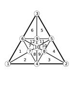
A popular split is the Powell-Sabin 12-split [Powell.Sabin77]; see Figure 1a and Section 3. While the 12-split splits the triangle in a relatively large number of subtriangles, a major advantage over other well-known splits stems from the following property [Oswald92, DynLyche98]. Let be given a triangle ![]() , its 12-split
, its 12-split ![]() , and the split
, and the split ![]() , where we subdivided
, where we subdivided ![]() into four subtriangles by connecting the midpoints of the edges. If we replace each subtriangle in
into four subtriangles by connecting the midpoints of the edges. If we replace each subtriangle in ![]() by its 12-split, the space of splines over the resulting split contains the space of splines over
by its 12-split, the space of splines over the resulting split contains the space of splines over ![]() . This refinability property makes the 12-split suitable for multiresolution analysis.
. This refinability property makes the 12-split suitable for multiresolution analysis.
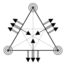
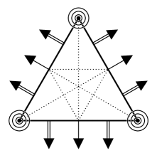
Recently, a simplex spline basis for the -quadratics on the 12-split with all the usual properties of the univariate B-spline basis was discovered [Cohen.Lyche.Riesenfeld13]. Powell and Sabin originally constructed a nodal basis (see Section 2) on the 12-split, which can be used to represent -smooth quadratic splines over arbitrary triangulations. Schumaker and Sorokina viewed the space of -quadratics on the 12-split as the first entry in a sequence of spline spaces of increasing smoothness and degree [Schumaker.Sorokina06]. The second entry is a space of -quintics, with -supersmoothness at the vertices and midpoints and satisfying some additional -conditions of type (4) along some of the interior edges. On a single triangle this space has dimension , and the authors constructed a nodal macro-element for this space; see Figure 2a.
For a recent and similar construction see [Davydov.Yeo13]. A family of smooth spline spaces on the 6-split and corresponding normalized bases were presented in [Speleers13]. For other refinable -quadratic elements on 6-splits see [D.L.M.S:S00, Maes.Bultheel06] and [Jia.Liu08]. In the latter a combination of 6- and 12-splits is used. For the FVS -cubic quadrangular macro element see [Davydov.Stevenson05, Hong.Schumaker04], and for a survey of refinable multivariate spline functions see [Goodman.Hardin06].
The next section reviews some standard Bernstein-Bézier techniques. Section 3 introduces a new macro-element space for -quintics, with complete -smoothness within each macrotriangle and dimension only ; see Figure 2b. In the following two sections a Hermite subdivision scheme is derived, implemented, and tested in the computer algebra system Sage. The final section concludes the paper.
2 Bernstein-Bézier techniques
We follow the notation from [Lai.Schumaker07]. Any point in a nondegenerate triangle can be represented by its barycentric coordinates , which are uniquely defined by and . Similarly, each vector is uniquely described by its directional coordinates, i.e., the triple with and the barycentric coordinates of two points and such that .
A polynomial of degree defined on is conveniently represented by its Bézier form
where the are referred to as the Bernstein basis polynomials of degree and the are called the B-coefficients of . We associate each B-coefficient to the domain point . The disk of radius around is , and similarly for the other vertices.
For any differentiable function and a vector (not necessarily of unit length), we write
for the directional derivative of along at . If, more generally, is -times differentiable for some integer , then, for any set of vectors , we write
for the -th order directional derivative in the directions of , and for its point evaluation at . We write
if . We shall make use of the short-hand
| (1) |
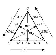
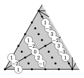
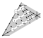
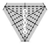
For any triangle there are some natural directions along which to consider directional derivatives. To any edge opposing the vertex , one associates the inward unit normal vector , tangential vector and the medial vector ; see Figure 1c. Since and are orthogonal,
| (2) |
The corresponding directional derivatives obey similar relations.
A linear functional is called nodal if it maps any spline to a linear combination of values and derivatives at a given point called the carrier of . A set of nodal functionals is called a nodal determining set for a spline space , if for all implies . If there is no smaller nodal determining set, is called minimal. We call a macro-element space provided that there is a nodal minimal determining set for such that for each triangle in the triangulation ![]() , is uniquely determined from the values , with the functionals with carrier in . In this case is a basis for the dual space of , and the dual basis to is called a nodal basis of . The functionals in are called degrees of freedom.
, is uniquely determined from the values , with the functionals with carrier in . In this case is a basis for the dual space of , and the dual basis to is called a nodal basis of . The functionals in are called degrees of freedom.
Suppose that and are triangles sharing the edge , and let
be polynomials defined on these triangles, where and are the Bernstein basis polynomials associated with and , respectively. Imposing a smooth join of and along translates into the linear relations among the B-coefficients presented in the following theorem.
Theorem 1.
Suppose is any direction not parallel to . Then
| (3) |
if and only if
| (4) |
where are the barycentric coordinates of with respect to . Moreover, if are collinear then (4) takes the form
| (5) |
which can also be written
| (6) |
where is the usual th order forward difference of , , and , .
Proof.
The equivalence of (3) and (4) follows from [Lai.Schumaker07, Thm. 2.28] by switching the order of the vertices and in . If are collinear, then and all terms with in (4) are zero. We obtain (5) with . It can be shown by induction on that (6) follows from (5). Alternatively it follows from univariate Bernstein-Bézier theory. ∎
Let us illustrate this theorem with several examples that will be used in the proof of Theorem 4.
Example 1.
Example 2.
Imposed values of the degrees of freedom translate into the linear relations among the B-coefficients presented in the following theorem; see e.g. [Lai.Schumaker07, Thm. 2.15].
Theorem 2.
Let , and suppose we are given, for , a vector with directional coordinates . Then
where and
As a consequence, for any , specifying all derivatives up to order at some vertex is equivalent to specifying the B-coefficients in the disk [Lai.Schumaker07, Thm. 2.18].
3 Macro-elements on Powell-Sabin splits
For the purpose of constructing approximations by piecewise quadratics, Powell and Sabin introduced two methods to split each triangle in a triangulation ![]() [Powell.Sabin77]. For the first of these, one considers a new vertex in the interior of each triangle in such a way that, for any triangles sharing an edge , the line segment intersects in a new point . For any edge on the boundary, one writes for the midpoint of . Inserting, for any edge and vertex of a triangle , the new vertices , and edges into , one arrives at a refined triangulation
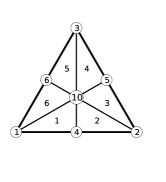
[Powell.Sabin77]. For the first of these, one considers a new vertex in the interior of each triangle in such a way that, for any triangles sharing an edge , the line segment intersects in a new point . For any edge on the boundary, one writes for the midpoint of . Inserting, for any edge and vertex of a triangle , the new vertices , and edges into , one arrives at a refined triangulation ![]() known as the Powell-Sabin 6-split of ; see Figure 1b.
known as the Powell-Sabin 6-split of ; see Figure 1b.
How should one choose the points so that each is well defined? If all triangles are acute one can choose to be the circumcenter of , and in general one can choose to be the incenter of [Lai.Schumaker03]. Alternatively, one can take the barycenter of each triangle , but this is only possible if the line-segment joining the barycenters of two adjacent triangles intersect the common edge. Alfeld and Schumaker [Alfeld.Schumaker02] avoid this geometric constraint by, for any edge shared by two adjacent triangles , choosing freely, no longer requiring to be collinear. This has the additional advantage that the choice of no longer affects the geometry of the split in any neighbouring macrotriangle.
The latter advantage is shared by the second split introduced by Powell and Sabin, which is constructed as follows. Given a triangle , write , , and for its edges. The midpoint of any edge is the average of its endpoints, and its quarterpoints are the averages and of the midpoint with the endpoints. We construct a 6-split by inserting a vertex at the barycenter, which we connect to the old vertices and the midpoints. Connecting the midpoints we arrive at the Powell-Sabin 12-split of ; see Figure 1a.
Let ![]() be a triangulation of some domain . Replacing every triangle in
be a triangulation of some domain . Replacing every triangle in ![]() by a 6-split (resp. 12-split) results in a finer triangulation
by a 6-split (resp. 12-split) results in a finer triangulation ![]() (resp.
(resp. ![]() ). We write (resp. ) for the space of piecewise quintic polynomials with global -smoothness on
). We write (resp. ) for the space of piecewise quintic polynomials with global -smoothness on ![]() (resp.
(resp. ![]() ) and -smoothness on each macrotriangle in
) and -smoothness on each macrotriangle in ![]() . We consider a set of functionals on , comprising point evaluations and partial derivatives up to order three at any vertex of
. We consider a set of functionals on , comprising point evaluations and partial derivatives up to order three at any vertex of ![]() . We also consider the superset of functionals on , which in addition contains, for each edge in
. We also consider the superset of functionals on , which in addition contains, for each edge in ![]() , a first-order cross-boundary derivative at the midpoint and a second-order cross-boundary derivative at each quarter point; see Figure 2b.
, a first-order cross-boundary derivative at the midpoint and a second-order cross-boundary derivative at each quarter point; see Figure 2b.
On a single triangle, one has and , matching the cardinalities of and . This can be computed numerically using a JAVA applet written by Peter Alfeld described in [Alfeld00] and available at http://www.math.utah.edu/~pa/MDS/. The dimension of the 6-split follows immediately from an “interior cell formula” [Lai.Schumaker07, Thm. 9.3], while the dimension of the 12-split follows from a formula for the dimension for general degree and smoothness , which we plan on reporting elsewhere.
Remark 3.
In Section 4 we derive a Hermite subdivision scheme for computing any spline from the initial data
| (7) |
Along any edge in , a third-order cross-boundary derivative at the midpoint cannot be determined from just the functionals along , as this would imply global -smoothness of . Since any spline has global -smoothness and -smoothness within each macrotriangle, the subdivision rules for the other derivatives at can only involve initial data along .
The following theorem shows that any spline is uniquely determined from the initial data (7).
Theorem 4.
The set forms a nodal minimal determining set for .
Proof.
For any vertex of ![]() , the derivatives up to order three at determine the disk . Along each edge of
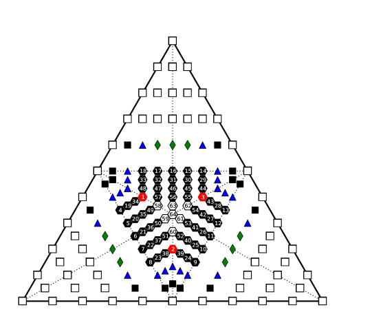
, the derivatives up to order three at determine the disk . Along each edge of ![]() , we therefore know the initial and final four B-coefficients. Therefore, since the space of -smooth quintic univariate splines along has dimension 8, the restriction of to is determined. Thus the nodal data at the corners determine the B-coefficients marked in Figure 4.
, we therefore know the initial and final four B-coefficients. Therefore, since the space of -smooth quintic univariate splines along has dimension 8, the restriction of to is determined. Thus the nodal data at the corners determine the B-coefficients marked in Figure 4.
Let and be the medial and tangential directions associated to . Since the space of -smooth quartic univariate splines along has dimension 7, the restriction of the cross-boundary derivative to is determined by its value at the mid-point and the 3 degrees of freedom at the corners . Specifying, in addition, a first-order cross-boundary derivative at each midpoint therefore determines the B-coefficients marked in Figure 4.
Similarly, since the space of -smooth cubic univariate splines along has dimension 6, the restriction of to is determined by its value at the 2 quarterpoints of and the 2 degrees of freedom at the corners . Specifying second-order cross-boundary derivatives at the quarterpoints therefore determines the B-coefficients marked in Figure 4.
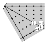
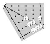
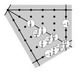
In order to show that these 39 conditions are independent, we need to determine the remaining B-coefficients from the smoothness conditions. For instance, using the smoothness conditions with coefficients shown in Figure 3d, one determines the B-coefficients marked in Figure 4.
Let us refer to the coefficients thus far as known. The remaining unknown coefficients are numbered as in Figure 4. By Theorem 2, determining is equivalent to determining a third-order cross-boundary derivative at the midpoint . By Remark 3, this derivative cannot be determined from only the initial data along the edge . For the time being, therefore, let us express in terms of and the known coefficients, writing if is a linear combination of known coefficients.
Using the univariate -condition from Figure 3e across the edge , one expresses in terms of . Similarly one expresses in terms of . The univariate smoothness conditions from Figure 3d along determine the remaining B-coefficients along this edge. Using the univariate smoothness conditions from Figure 3e across the edge , and similar relations for , one obtains
Similar expressions hold for the other unknown B-coefficients outside of . Using the -condition from Figure 3a across (and similarly for and ),
and taking averages of these coefficients (as the -condition in Figure 3d),
Using any -condition at (e.g. Figure 3a), we find .
At this point all unknown B-coefficients are expressed in terms of . The univariate -condition along from Figure 3f (and similarly for , ) yield
so that . Substituting in the -condition from Figure 3c,
determines the remaining degree of freedom in terms of the known B-coefficients.
Finally, since the univariate splines , and are determined from just the functionals along , the values, first, and second derivatives of the splines on the adjacent triangles agree along . It follows that defines a spline that is -smooth on ![]() and -smooth on each macro-triangle in
and -smooth on each macro-triangle in ![]() .
∎
.
∎
Similarly, any spline is uniquely determined from the initial data
| (8) |
which follows from combining Theorem 2.18 and 7.9 in [Lai.Schumaker07]:
Theorem 5.
The set forms a nodal minimal determining set for .
4 Derivation of a subdivision scheme
It has been observed by many (see e.g. [DynLyche98, Oswald92]) that the geometry of the 12-split lends itself for subdivision into four subtriangles, namely , , , and in Figure 1a. Each of these is (refinable to) a 6-split. Moreover, splitting the 6-split in Figure 1b into four subtriangles yields four new 6-splits, etc. Using this observation, one can derive a Hermite subdivision scheme to compute the -smooth quadratic splines from values and first derivatives at the corners and cross-boundary derivatives at the midpoints [DynLyche98].
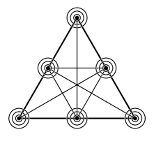
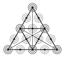
In this section we derive a similar scheme for computing any spline from the initial data (7). After computing the values and derivatives at the midpoints in the “initialization step” in Figure 5a, one obtains a refined description of by repeatedly applying the “subdivision step” in Figure 5b.
Remark 6.
For two adjacent triangles with common edge , specifying cross-boundary derivatives in the normal direction at the midpoints and quarterpoints has the advantage of only depending on the common edge. However, since tangential derivatives at the midpoints and quarterpoints can easily be computed from the tangential derivatives at the corners (see (2) and the rules below), any other directional derivative can be computed by a simple change of basis.
To keep the rules as short as possible, we specify directional derivatives in the medial directions and tangential directions . Because the edges in the 12-split are divided at the midpoints, each of the four subdivided triangles in Figure 5b will have the same tangential and medial vectors, albeit scaled by a factor . Thus directional derivatives computed on previous levels can be reused.
It follows from Theorem 4 (resp. Theorem 5) that the B-coefficients of any spline in (resp. ) can be uniquely determined from the initial data (7) (resp. (8)). Moreover, Theorem 2 implies that any directional derivative of any order of the spline at any point can be expressed in terms of the B-coefficients. It follows that there exist initialization rules and subdivision rules for evaluating the spline as described above. In the next two sections we derive these rules.
By Remark 3, the initialization and subdivision rule for the third-order cross-boundary derivative at the midpoint is expected to be complicated, involving functionals with carrier outside of . Because of this, the formulas for the case of (locally) -quintics are considerably more complex than those for the -quadratics. As the computations are too large to carry out by hand, we made use of the computer algebra system Sage [Sage]. The resulting worksheet with implementation and examples can be downloaded from the website of the second author [WebsiteGeorg].
Initialization
On a single triangle ![]() , with the 252 unknown B-coefficients
, with the 252 unknown B-coefficients
the initial conditions (7) and smoothness conditions (4) for the 15 interior edges in ![]() form a linear system with equations. By the linear independence of the functionals in , this system has a unique solution. Solving the system and applying Theorem 2, we find initialization rules for computing the data in Figure 5a from the initial data (7).
form a linear system with equations. By the linear independence of the functionals in , this system has a unique solution. Solving the system and applying Theorem 2, we find initialization rules for computing the data in Figure 5a from the initial data (7).
Given are, at the corners , values and derivatives of up to order three, first-order cross-boundary derivatives at the midpoints, and second-order cross-boundary derivatives
at the quarter points as in Figure 2b. With the short-hands , and (1), the value and derivatives at the midpoint are determined by the rules (see the worksheet)
Note that only the third-order cross-boundary derivative involves functionals with carrier outside of , as explained in Remark 3.
Subdivision
On a single triangle ![]() , with the 126 unknown B-coefficients
, with the 126 unknown B-coefficients
the initial conditions (8) and smoothness conditions (4) for the 6 interior edges in ![]() form a linear system with equations. By the linear independence of the functionals in , this system has a unique solution. Solving the system and applying Theorem 2, we find subdivision rules for computing the dashed data in Figure 5b from the data in Figure 5a (see the worksheet),
form a linear system with equations. By the linear independence of the functionals in , this system has a unique solution. Solving the system and applying Theorem 2, we find subdivision rules for computing the dashed data in Figure 5b from the data in Figure 5a (see the worksheet),
Remark 7.
Taking convex combinations of the rules for the -quadratic and -quintic schemes, one arrives at a family of Hermite interpolatory subdivision schemes. A general member of this family will produce limit functions that are not piecewise polynomial.
5 Implementation and experimentation
In this section we apply the scheme to compute some example splines in some example triangulations. For details we refer to the Sage worksheet.


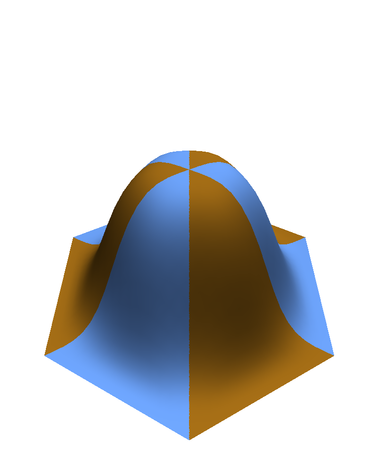
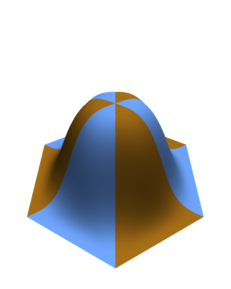
Example 3.
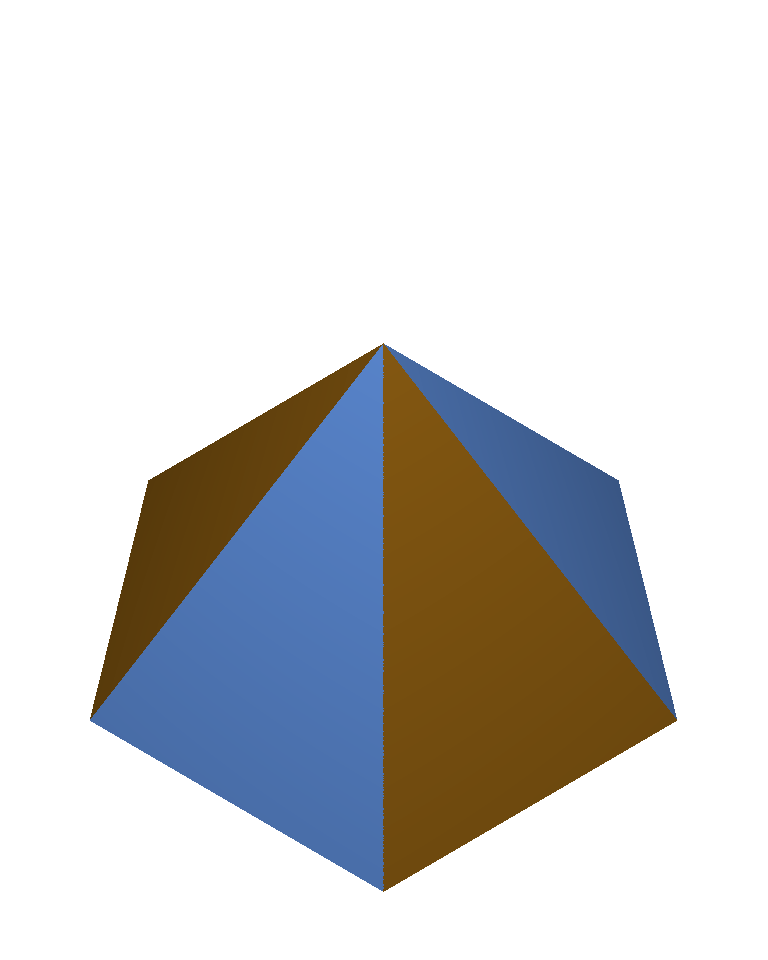
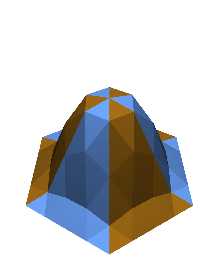
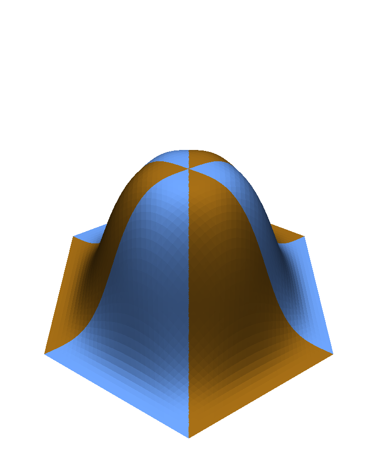
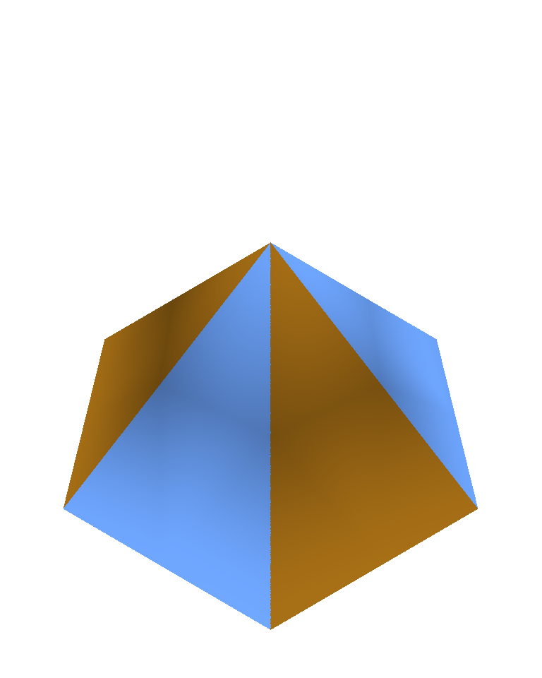
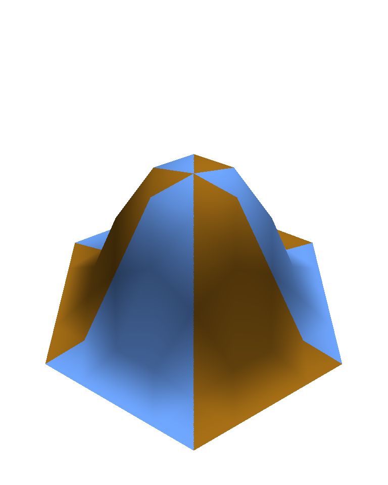
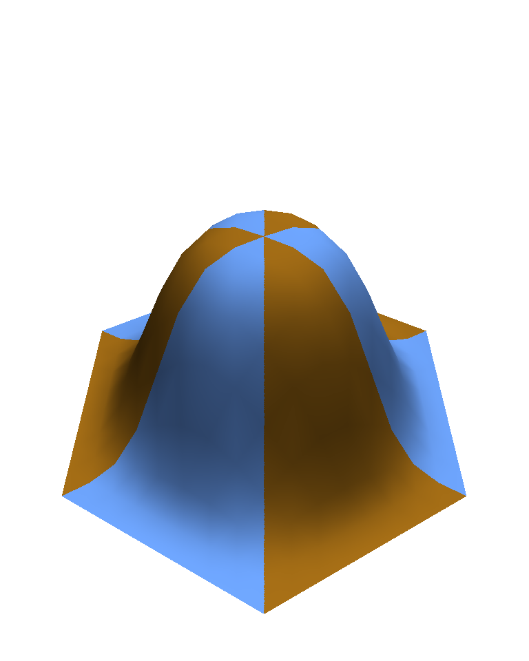
Let , with , be the vertices of a regular hexagon centred at the origin . Consider the triangulation consisting of the triangles , with , and . We consider the spline on this triangulation defined by zero initial data in (7), except for the value for the point evaluation at .
After the initialization step, the first 5 iterations of the subdivision step are shown in the top row of Figure 6. However, in general we do not need this many iterations. Since the Hermite subdivision scheme also computes first derivatives, we know the surface normal at each vertex. Linearly interpolating these normals along each triangle and ray-tracing with a Phong shading model yields a seemingly flawless visualization after 2-3 iterations, while for flat shading 4-5 iterations are needed; see Figure 6 for a comparison.
Example 4.
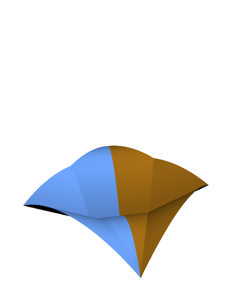
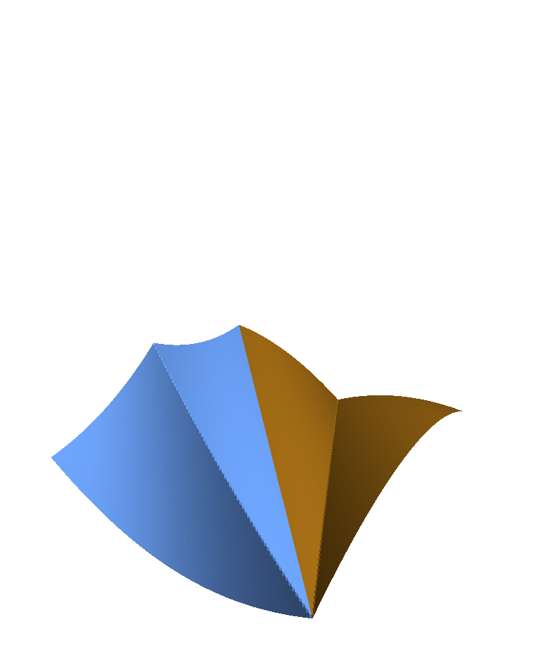
Consider the triangulation ![]() with two triangles and , with
with two triangles and , with
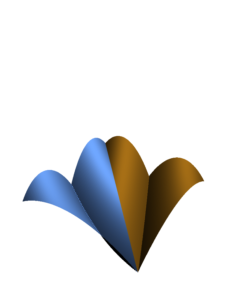
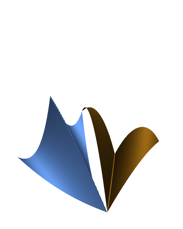
We consider the spline on this triangulation defined by zero initial data in (7), except for the value for the point evaluation at . Since the Hermite scheme computes derivatives up to order three, it is easy to plot the third derivatives of in Figure 7. Note that all third derivatives are continuous on ![]() , with the exception of the third-order cross-boundary derivative , as expected.
, with the exception of the third-order cross-boundary derivative , as expected.
Applying the scheme to data sampled from a random quintic polynomial on ![]() reproduced this polynomial exactly in exact arithmetic, and up to machine accuracy in floating point arithmetic.
reproduced this polynomial exactly in exact arithmetic, and up to machine accuracy in floating point arithmetic.
6 Conclusion and a final remark
We have introduced a nodal macro-element on the 12-split for the space of quintic splines that are locally and globally . For quickly evaluating any such spline, a Hermite subdivision scheme is derived, implemented, and tested in the computer algebra system Sage. Using the available first derivatives for Phong shading, visually appealing plots can be generated after just a couple of refinements.
Remark 8.
It would be natural to consider the macro-element introduced by Powell and Sabin and the macro-element in this paper as the first two entries in the following sequence. Let be the space of piecewise polynomials of degree with global -smoothness and -smoothness within each macro-triangle. We define a set of functionals on as follows. For every vertex of ![]() , the set contains point evaluations at of the spline and of its partial derivatives up to order . The remaining elements of are, for each edge in
, the set contains point evaluations at of the spline and of its partial derivatives up to order . The remaining elements of are, for each edge in ![]() and , point evaluations of cross-boundary derivatives of order along .
and , point evaluations of cross-boundary derivatives of order along .
Although the cardinality of matches , which can be shown to be , it unfortunately does not in general form a basis for the dual to . The pattern breaks down first for , for which has dimension . While on each macro-triangle the 81 functionals in are linearly independent in the space of -smooth octics, they are dependent in the space of -smooth octics, with corank three.
7 Acknowledgments
We wish to express our gratitude to the referees for their useful comments, which helped to improve the presentation of this paper. The second author was supported by a FRINATEK grant, project number 222335, from the Research Council of Norway.