Warm Anisotropic Inflationary Universe Model

Abstract

This paper is devoted to study the warm inflation using vector fields in the background of locally rotationally symmetric Bianchi type I universe model. We formulate the field equations, slow-roll and perturbation parameters (scalar and tensor power spectra as well as their spectral indices) under slow-roll approximation. We evaluate all these parameters in terms of directional Hubble parameter during intermediate and logamediate inflationary regimes by taking the dissipation factor as a function of scalar field as well as a constant. In each case, we calculate the observational parameter of interest, i.e., tensor-scalar ratio in terms of inflation. The graphical behavior of these parameters shows that the anisotropic model is also compatible with WMAP7 and Planck observational data.

Keywords: Vector fields; Warm inflation; Slow-roll approximation.
PACS: 98.80.Cq; 05.40.+j.

1 Introduction

In the context of cosmology, it has become an inevitable fact through the combined efforts of type Ia Supernova, the large scale structure (LSS), cosmic microwave background (CMB) and WMAP that universe is undergoing a stage of accelerating expansion [1]. This cosmic behavior might be due to the repulsive nature of missing energy (due to the large negative pressure) called dark energy (DE) which occupies 70 percent of the universe. It is described by a tiny time-independent cosmological constant $(\Lambda)$ obeying $\omega=-1$ ($\omega$ is the equation of state (EoS) parameter). Due to the fine-tuning and cosmic coincidence issues [2] of this constant, the search for variety of DE models is ongoing. The dynamical nature of DE is divided into two categories: scalar field models (quintessence, phantom with negative kinetic term, k-essence, quintom (unification of quintessence and phantom) etc.) [3] and interacting DE models (Chaplygin gas having novel EoS, holographic DE, Ricci DE etc.) [4].

The standard cosmology (big-bang model) successfully explains the observations of CMB radiations but still there are some unresolved issues. The early universe is facing some long standing problems including horizon problem (why is the universe isotropic and homogeneous on large scale structure?), flatness (why is $\Omega_{total}\approx 1$ today?), monopole issue (why do not they exist?) and finally what is the origin of the fluctuations? [5]. The inflationary scenario $(\omega<-\frac{1}{3})$ proved to be a cornerstone to explain the mechanism of the early universe and provides the most compelling solution of these problems. The constant $\Lambda$ can also resolve these issues but unfortunately, in this case inflation never ends and the normal cosmos evolution remains impossible.

Scalar field (composed of kinetic and potential terms coupled to gravity) is the perfect candidate to produce the dynamical framework and acts as a source for inflation. In field theory, a spin zero particle is usually defined by a scalar field whereas mathematically, it is a function of space and time. It has ability to interpret the distribution of LSS and the observed anisotropy of the CMB radiations elegantly in inflationary era [6]. Golovnev et al. [7] discussed the vector inflation models based on orthogonal triplet and non-minimally coupled to gravity which show the similar behavior as the scalar fields in a flat universe.

The inflation regime is divided into two parts, i.e., slow-roll and reheating epochs. During slow-roll period, the universe inflates as the interactions among scalar fields while other fields become meaningless and potential energy dominates the kinetic term [8]. Reheating is the end stage of the inflation where kinetic and potential energies are comparable and universe starts oscillating about minimum potential [9]. Warm inflation [10] has an attractive feature of joining the expanding universe with the end of vector inflation. This motivated researchers to discuss the inflationary scenario in the context of warm inflation. During this regime, the dissipation effects become strong enough due to the production of thermal fluctuations of constant density which play a vital role in the formation of initial fluctuations necessary for LSS construction. An additional advantage of warm vector inflation is that the universe stops inflating and smoothly enters into the radiation dominated phase [11].

Inflation is usually discussed in the context of intermediate and logamediate scenarios. Intermediate inflation is motivated by string or M theory and proved to be the exact solution of the inflationary cosmology containing a particular form of the scale factor [12]. In intermediate era, the universe expands at the rate slower than the standard de Sitter inflation $(a=a_{0}\exp(H_{0}t);\quad a_{0},~{}H_{0}>0)$ while faster than power-law inflation $(a=t^{m},\quad m>1)$ [13]. On the other hand, the logamediate inflation [14] is motivated by applying weak general conditions on the indefinite expanding cosmological models. Barrow [15] applied this scenario to constant, power-law as well as exponential types of scalar field. The effective potential and various types of potential associated with this model are used in different DE models and in supergravity, Kaluza-Klein as well as string theories, respectively [16]. It has been proved that the power spectrum is red or blue tilted for this type of inflation.

In a recent paper [17], Setare and Kamali have discussed the warm vector inflation in intermediate as well as logamediate scenarios for FRW model and proved the physical compatibility of these results with WMAP7 data [16] through the perturbed parameters. In this paper, we study the above mentioned scenario in the framework of anisotropic universe model, i.e., locally rotationally symmetric (LRS) Bianchi I (BI). The format of the paper is as follows. In the next section, we construct the field equations from action and calculate the corresponding pressure as well as energy density imposing slow-roll condition. We also formulate the slow-roll as well as scalar and tensor perturbed parameters. In section 3, we evaluate the Hubble parameter, scalar field as well as slow-roll and perturbed parameters in two regimes (i) intermediate inflation (ii) logamediate inflation. The inflationary universe is further studied with variable and constant dissipation factor. The results are summarized in section 4.

2 Basic Formalism and Perturbations

In this section, we briefly discuss the inflationary model using the anisotropic background of the universe. A massive vector field, non-minimally coupled to gravity is presented by the following action [7]

$$\mathcal{S}=-\frac{1}{2}\int d^{4}x\sqrt{-g}(R+\frac{1}{2}F_{\alpha\beta}F^{\alpha\beta}-\frac{R}{6}A^{\alpha}A_{\alpha}-V(A^{\alpha}A_{\alpha})),$$

where $\alpha,\beta=0,1,2,3$, the field strength $(F_{\alpha\beta})$ and potential $(V)$ are defined as follows

$$F_{\alpha\beta}=\partial_{\alpha}A_{\beta}-\partial_{\beta}A_{\alpha},\quad V(A^{\alpha}A_{\alpha})=m^{2}A^{\alpha}A_{\alpha}+\ldots$$

This non-minimal coupling of the vector field has an opposite effect, i.e., it violates the conformal invariance of the massless vector field and forces it to behave just like a minimally coupled scalar field. The variation of the action with respect to $A_{\alpha}$ yields the following equations of motion

$$\frac{1}{\sqrt{-g}}\partial_{\alpha}(\sqrt{-g}F^{\alpha\beta})+\frac{R}{6}A^{\beta}+\frac{\partial V}{\partial A_{\beta}}=0,$$ (1)

where $\partial_{\alpha}=\frac{\partial}{\partial x^{\alpha}}$. An isotropic model (FRW) is unsteady near the initial singularity thus unable to explain the early mechanism of the universe. There is a need of an appropriate geometry which is more concise and general than the isotropic and homogeneous FRW universe. Bianchi models are prime and viable models to discuss the behavior of the early universe. A BI model being the straightforward generalization of the flat FRW model is one of the simplest models of the anisotropic universe.

The line element for LRS BI model $(b(t)=c(t))$ is given as

$$ds^{2}=-dt^{2}+a^{2}(t)dx^{2}+b^{2}(t)(dy^{2}+dz^{2}),$$

where $a(t),~{}b(t)$ are the scale factors along $x$-axis and $(y,z)$-axis, respectively. This metric can be transformed in the following form using a linear relationship $a=b^{n},~{}n\neq 1$ [18]

$$ds^{2}=-dt^{2}+b^{2n}(t)dx^{2}+b^{2}(t)(dy^{2}+dz^{2}).$$ (2)

In this scenario, Eq.(1) leads to

$$\ddot{A}_{i}+(\frac{n+2}{3})b^{\frac{(n-4)}{3}}\dot{b}(\dot{A}_{i}-\partial_{i}A_{0})+\frac{1}{b^{\frac{2(n+2)}{3}}}(\partial_{i}(\partial_{k}A_{k})-\Delta A_{i})-\partial_{i}\dot{A_{0}}+(m^{2}+\frac{R}{6})A_{i}=0,$$

$$-b^{-\frac{2(n+2)}{3}}\Delta A_{0}+(m^{2}+\frac{R}{6})A_{0}+b^{-\frac{2(n+2)}{3}}\partial_{i}\dot{A}_{i}=0,$$ (3)

where dot represents the time rate of change. Applying the condition of homogeneous vector field, i.e., $\partial_{i}A_{\alpha}=0$ to Eq.(3), one can deduce $A_{0}=0$. Another variable $\mathcal{B}_{i}=\frac{A_{i}}{b^{\frac{n+2}{3}}}$ is introduced for scalar field in place of $A_{i}$. Consequently, Eq.(3) has the similar form as the massive minimally coupled scalar field which can be written as

$$\ddot{\mathcal{B}}_{i}+(n+2)H_{2}\dot{\mathcal{B}}_{i}+V^{\prime}(\mathcal{B}_{j}\mathcal{B}^{j})\mathcal{B}_{i}=0,$$

or equivalently

$$\ddot{\mathcal{B}}_{i}+(n+2)H_{2}\dot{\mathcal{B}}_{i}+m^{2}\mathcal{B}_{i}=0,$$ (4)

where $H_{2}=\frac{\dot{b}}{b}$ is the directional Hubble parameter and prime denotes derivative with respect to $\mathcal{B}_{j}\mathcal{B}^{j}$.

The corresponding energy-momentum tensor can be obtained by varying the action with respect to the metric $(g^{\alpha\beta})$ [7]. The temporal and the spatial components of energy-momentum tensor are

$$T^{0}_{0} = \frac{1}{2}(\dot{\mathcal{B}}^{2}_{k}+V(\mathcal{B}^{i}\mathcal{B}_{i})),$$

$$T^{i}_{j} = \left[-\frac{5}{6}\dot{\mathcal{B}}^{2}_{k}+\frac{1}{2}V(\mathcal{B}^{2})-\frac{2}{3}\left(\frac{n+2}{3}\right)H_{2}\dot{\mathcal{B}}_{k}\mathcal{B}_{k}-\frac{1}{3}\left(\left(\frac{n+2}{3}\right)\dot{H}_{2}\right.\right.$$ (5)

$$+ \left.\left.3\left(\frac{n+2}{3}\right)^{2}H^{2}_{2}-V^{\prime}(\mathcal{B}^{2})\right)\mathcal{B}^{2}_{k}\right]{\delta}^{i}_{j}+\dot{\mathcal{B}}_{i}\dot{\mathcal{B}}_{j}+\left(\frac{n+2}{3}\right)H_{2}(\dot{\mathcal{B}}_{i}\mathcal{B}_{j}+\dot{\mathcal{B}}_{j}\mathcal{B}_{i})$$

$$+ \left(\left(\frac{n+2}{3}\right)\dot{H}_{2}+3\left(\frac{n+2}{3}\right)^{2}H^{2}_{2}-V^{\prime}(\mathcal{B}^{2})\right)\mathcal{B}_{i}\mathcal{B}_{j},$$

where $k$ stands for summation index and $\mathcal{B}_{k}$ satisfies Eq.(4) for any vector field. We have considered the LRS BI universe model with homogeneous vector field which does not contain the off-diagonal terms in the energy-momentum tensor. In order to make the spatial component of the energy-momentum tensor diagonal, we use various fields simultaneously. Therefore, a triplet of the mutually orthogonal vector fields is defined as follows [19]

$$\sum_{a}\mathcal{B}^{a}_{i}\mathcal{B}^{a}_{j}=|\mathcal{B}|^{2}{\delta}^{j}_{i}.$$

Using the above conditions with an ansatz, $\mathcal{B}^{a}_{i}=|\mathcal{B}|{\delta}^{a}_{i}$ in Eq.(5), the components of the energy-momentum tensor reduce to diagonal form as

$$T^{0}_{0} = \rho_{v}=\frac{3}{2}(\dot{\mathcal{B}}^{2}_{k}+V(|\mathcal{B}|^{2})),$$

$$T^{i}_{j} = -P_{v}{\delta}^{i}_{j}=-\frac{3}{2}(\dot{\mathcal{B}}^{2}_{k}-V(|\mathcal{B}|^{2})){\delta}^{i}_{j}.$$

These equations are similar to the equations which are evaluated in [20] for massive scalar field. The choice of $|\mathcal{B}|>1$ corresponds to the inflation epoch under slow-roll limit $(\dot{\mathcal{B}}^{2}_{k}\ll V(\mathcal{B}^{2}))$ for which $\rho_{v}=-P_{v}$.

We assume that the total energy density of the universe is the sum of energy density of the vector field $(\rho_{v})$ and radiation $(\rho_{\gamma})$. The mechanism of warm vector inflation can be represented by the first field equation (evolution equation) and conservation equations given as

$$H^{2}_{2}=\frac{1}{1+2n}(\frac{3}{2}(\dot{\mathcal{B}}^{2}_{k}+V(|\mathcal{B}|^{2}))+\rho_{\gamma}) = \frac{1}{1+2n}(\rho_{v}+\rho_{\gamma}),$$

$$\dot{\rho_{v}}+(n+2)H_{2}(\rho_{v}+P_{v}) = -\eta\dot{\mathcal{B}}^{2},$$

$$\dot{\rho}_{\gamma}+\frac{4(n+2)}{3}H_{2}\rho_{\gamma} = \eta\dot{\mathcal{B}}^{2},$$ (6)

where $\eta,~{}T_{\gamma}$ stand for dissipation or friction factor and temperature of the thermal bath, respectively. We assume a suitable form of $\eta=\eta_{0}\frac{T_{\gamma}^{3}}{\mathcal{B}^{2}}$, where $\eta_{0}$ is any constant and $T_{\gamma}$ can be extracted via quantum field theory method which holds for low temperature [21]. In this method, the inflation interacts with heavy intermediate field (acts as catalyst) which could decay into massless field called radiation. Here $\eta$ is taken to be positive (by second law of thermodynamics) which implies that the energy density of scalar field decays into radiation density. During inflation era, $\rho_{v}\sim V(A^{2})$ and the energy density of inflation exceeds to radiation density $(\rho_{v}>\rho_{\gamma})$. Further, we apply two limits on the above dynamic equations, i.e., slow-roll approximation $(\ddot{\mathcal{B}}\ll((n+2)H_{2}+\frac{\eta}{3})\dot{\mathcal{B}})$ and quasi-stability of the radiation production where $\dot{\rho_{\gamma}}\ll 4(\frac{n+2}{3})H_{2}\rho_{\gamma},~{}\dot{\rho_{\gamma}}\ll\eta\dot{\mathcal{B}}^{2}$ [10]. Using all these conditions, we can write Eq.(6) as follows

$$-\frac{1}{2}V^{\prime} = (n+2)(1+\frac{\chi}{3})H_{2}\dot{\mathcal{B}},$$ (7)

$$\rho_{\gamma} = \frac{3}{4}\chi\dot{\mathcal{B}}^{2}=\frac{(1+2n)}{8(n+2)^{2}}\frac{\chi}{(1+\frac{\chi}{3})^{2}}\frac{{V^{\prime}}^{2}}{V}=C_{\gamma}T_{\gamma}^{4},$$ (8)

$$H^{2}_{2} = \frac{3}{2(1+2n)}V,$$ (9)

where $\chi=\frac{\eta}{(n+2)}H_{2}$ denotes the rate of dissipation which represents strong $(\chi>1)$ and weak $(\chi<1)$ dissipation regions. The radiation energy density is also written in the form $C_{\gamma}T_{\gamma}^{4}$, where $C_{\gamma}=\frac{\pi^{2}g_{\ast}}{30}$ and $g_{\ast}$ is known as the number of relativistic degrees of freedom. Using Eqs.(7) and (9) in (8), the temperature of thermal bath can be obtained as follows

$$T_{\gamma}=\left[\frac{-(1+2n)\chi\dot{H}_{2}}{2C_{\gamma}(n+2)(1+\frac{\chi}{3})}\right]^{\frac{1}{4}}.$$ (10)

The dimensionless slow-roll parameters $(\epsilon,~{}\lambda)$ [22] of the warm vector inflation can be calculated using Eq.(9) as

$$\epsilon = -\frac{3}{(n+2)H_{2}}\frac{d}{dt}\left(\ln\left(\frac{n+2}{3}H_{2}\right)\right)=-\frac{3}{(n+2)}\frac{\dot{H}_{2}}{H^{2}_{2}}$$ (11)

$$= \frac{1+2n}{2(n+2)^{2}(1+\frac{\chi}{3})}\frac{{V^{\prime}}^{2}}{V^{2}},$$

$$\lambda = -\frac{3}{(n+2)}\frac{\ddot{H}_{2}}{H_{2}\dot{H}_{2}}=2\epsilon-\frac{3\dot{\epsilon}}{(n+2)H_{2}\epsilon}$$ (12)

$$= 2\epsilon+\frac{6(1+2n)}{(n+2)^{2}(3+\chi)}\left(\frac{V^{\prime}}{V}\right)\left[\frac{V^{\prime\prime}}{V^{\prime}}-\frac{V^{\prime\prime}}{V}-\frac{3}{2}\frac{\chi^{\prime}}{(3+\chi)}\right].$$

The energy density of the scalar field can be expressed in terms of radiation density using Eqs.(9) and (11) as

$$\rho_{\gamma}=\frac{1}{2}\left(\frac{\chi}{3+\chi}\right)\epsilon\rho_{v}.$$

Here, we consider strong dissipative regime where $\chi\gg 1$ which implies that $\eta\gg 3(n+2)H_{2}$. Consequently, $\rho_{\gamma}$ can be simplified as

$$\rho_{\gamma}=\frac{1}{2}\epsilon\rho_{v}.$$ (13)

The condition of the warm inflation epoch, i.e., $\rho_{v}>2\rho_{\gamma}$ can be verified via an inequality $0<\ddot{b}<1$ for which $\epsilon<1$. This inflationary scenario ends at $\epsilon=1$ where the field energy density becomes twice of the radiation density. The number of e-folds at two different cosmological times $t$ (beginning of inflation) and $t_{1}$ (end of inflation) is defined as follows

$$N=\frac{(n+2)}{3}\int^{t_{1}}_{t}H_{2}dt=-\frac{(n+2)^{2}}{2(1+2n)}\int^{t_{1}}_{t}(3+\chi)\frac{V}{V^{\prime}}dt.$$ (14)

Now we evaluate scalar and tensor perturbations for anisotropic LRS BI universe model at small scale structure by varying the field $\mathcal{B}$. In non-warm and warm inflation, quantum and thermal fluctuations, respectively yield [23]

$$\langle\delta\mathcal{B}\rangle_{quantum}=\left(\frac{n+2}{3}\right)^{2}\frac{H^{2}_{2}}{2\pi},\quad\langle\delta\mathcal{B}\rangle_{thermal}=\left(\frac{n+2}{3(4\pi)^{3}}\right)^{\frac{1}{4}}(\eta H_{2}T_{\gamma}^{2})^{\frac{1}{4}}.$$ (15)

In cosmology, a useful function of wave number $(k)$, known as power spectrum is introduced to quantify the variance in the fluctuations due to inflation. In warm inflationary universe, the scalar power spectrum is given by [24]

$$\Delta^{2}_{R}(k)=\left(\frac{n+2}{3}\right)^{2}\left(\frac{H_{2}}{\dot{\mathcal{B}}}\langle\delta\mathcal{B}\rangle_{thermal}\right)^{2}.$$ (16)

Using Eqs.(6), (9) and (15), we can calculate the power-spectrum of scalar perturbation in the form

$$\Delta^{2}_{R}(k)=-\left[\frac{(n+2)^{5}\eta^{3}T_{\gamma}^{2}}{972(1+2n)^{2}(4\pi)^{3}}\right]^{\frac{1}{2}}\frac{H^{\frac{3}{2}}_{2}}{\dot{H}_{2}}=\left[\frac{(n+2)^{5}\eta^{5}T_{\gamma}^{2}}{6^{\frac{3}{2}}972(1+2n)^{\frac{5}{2}}(4\pi)^{3}}\right]^{\frac{1}{2}}\frac{V^{\frac{5}{4}}}{{V^{\prime}}^{2}}.$$ (17)

The second important parameter to study the fluctuations is the scalar spectral index $(n_{s})$. For the present model, it is defined as

$$n_{s}-1=-\frac{d\ln\Delta^{2}_{R}(k)}{d\ln k}.$$ (18)

The tensor perturbation $(\Delta^{2}_{T}(k))$ and its spectral index $(n_{T})$ for anisotropic universe are

$$\Delta^{2}_{T}(k) = \left(\frac{n+2}{3\pi}\right)^{2}H^{2}_{2}=\left(\frac{(n+2)^{2}}{3(1+2n)}\right)\frac{V}{\pi^{2}},$$ (19)

$$n_{T} = -2\epsilon.$$ (20)

The tensor-scalar ratio $(R)$ has the following form

$$R=-\left[\frac{48(1+2n)(4\pi)^{3}}{(n+2)\pi^{4}\eta^{3}T_{\gamma}^{2}}\right]^{\frac{1}{2}}H^{\frac{1}{2}}_{2}\dot{H}_{2}.$$ (21)

According to the observations of WMAP+BAO+SN, the perturbed scalar power spectrum is constrained to $\Delta^{2}_{R}(k_{0}=0.002Mpc^{-1})=(2.445\pm 0.096)\times 10^{-9}$ [6]. In this context, the physical acceptable range of scalar-tensor ratio is determined, i.e., $R<0.22$ representing the expanding universe.

3 Intermediate and Logamediate Inflation

In this section, we discuss the warm vector inflation in the context of intermediate and logamediate inflations by treating $\eta$ as a function of $\mathcal{B}$ as well as a constant.

3.1 Intermediate Inflation

In intermediate scenario, the scale factor follows the law [12]

$$b(t)=b_{0}\exp(\mu t^{g}),\quad\mu>0,~{}0<g<1.$$ (22)

The number of e-folds for this model can be calculated using Eq.(14) as

$$N=\frac{(n+2)}{3}\mu(t^{g}-t^{g}_{1}).$$ (23)

Firstly, we explore the dynamics of the warm intermediate inflation by considering the variable dissipation factor.

3.1.1 Case 1: $\eta=\eta_{0}\frac{T_{\gamma}^{3}}{\mathcal{B}^{2}},~{}\eta_{0}=constant$

Here, we evaluate some quantities which are useful to determine the parameters defined in the previous section. The scalar potential is evaluated in terms of cosmic time $t$ using Eq.(9) as

$$V=\frac{2(1+2n)}{3}(\mu g)^{2}t^{2(g-1)}.$$ (24)

The scalar field and the directional Hubble parameter are found using Eqs.(7), (9), (10) and (24) as follows

$$\mathcal{B}=\mathcal{B}_{0}\exp(\omega_{0}t^{\frac{5g+2}{8}}),\quad H_{2}=\mu g\left(\frac{\ln\mathcal{B}-\ln\mathcal{B}_{0}}{\omega_{0}}\right)^{\frac{8(g-1)}{5g+2}},$$ (25)

where $\omega_{0}=[\frac{2}{3\eta_{0}}(\frac{1+2n}{n+2})^{\frac{1}{4}}(\frac{2C_{\gamma}}{3})^{\frac{3}{4}}]^{\frac{1}{2}}\frac{(1-g)^{\frac{1}{8}}(\mu g)^{\frac{5}{8}}}{5g+2}$ is a pure constant. In this context, the slow-roll parameters take the form

$$\epsilon = \left(\frac{3}{n+2}\right)\frac{1-g}{\mu g}\left(\frac{\ln\mathcal{B}-\ln\mathcal{B}_{0}}{\omega_{0}}\right)^{\frac{-8g}{5g+2}},$$

$$\lambda = \left(\frac{3}{n+2}\right)\frac{2-g}{\mu g}\left(\frac{\ln\mathcal{B}-\ln\mathcal{B}_{0}}{\omega_{0}}\right)^{\frac{-8g}{5g+2}}.$$ (26)

The radiation density (13) can be calculated in terms of scalar field as

$$\rho_{\gamma}=\frac{3(1+2n)}{2}\epsilon H^{2}_{2}=\frac{9(1+2n)}{2(n+2)}(\mu g)(1-g)\left(\frac{\ln\mathcal{B}-\ln\mathcal{B}_{0}}{\omega_{0}}\right)^{\frac{8(g-2)}{5g+2}}.$$ (27)

Inflationary era $(\epsilon<1)$ has the scalar field of magnitude $\mathcal{B}$.

We assume that $\mathcal{B}_{1}$ is another field which is produced at the end of inflation and could be found by fixing $\epsilon=1$ as

$$\mathcal{B}_{1}=\mathcal{B}_{0}\exp\left[\omega_{0}\left(\frac{3(1-g)}{(m+2)\mu g}\right)^{\frac{5g+2}{8g}}\right].$$

Inserting the values of two different cosmic times (using $\mathcal{B}$ and $\mathcal{B}_{1}$) in Eq.(23), we get

$$N=(\frac{n+2}{3})\mu\left[\left(\frac{\ln\mathcal{B}-\ln\mathcal{B}_{0}}{\omega_{0}}\right)^{\frac{8(g-2)}{5g+2}}-\left(\frac{\ln\mathcal{B}_{1}-\ln\mathcal{B}_{0}}{\omega_{0}}\right)^{\frac{8(g-2)}{5g+2}}\right].$$

These two equations yield $\mathcal{B}$ in terms of $N$ in the following form

$$\mathcal{B}=\mathcal{B}_{0}\exp\left[\omega_{0}\left(\left(\frac{3}{n+2}\right)\left(\frac{N}{\mu}+\frac{1-g}{g\mu}\right)\right)^{\frac{5g+2}{8g}}\right].$$ (28)

Using Eqs.(10) and (25) in (17), the perturbed scalar power spectrum in warm vector intermediate inflation (can also be expressed in terms of e-folds with the help of Eq.(28)) is

$$\Delta^{2}_{R}(k) = \left(\frac{\eta^{3}_{0}}{972(4\pi)^{3}}\right)^{\frac{1}{2}}\left[\frac{3^{11}(n+2)^{29}(\mu g)^{15}(1-g)^{3}}{(2C_{\gamma})^{11}(1+2n)^{5}}\right]^{\frac{1}{8}}\mathcal{B}^{-3}$$

$$\times \left(\frac{\ln\mathcal{B}-\ln\mathcal{B}_{0}}{\omega_{0}}\right)^{\frac{15g-18}{5g+2}}$$

$$= \left(\frac{\eta^{3}_{0}}{972(4\pi)^{3}}\right)^{\frac{1}{2}}\left[\frac{3^{11}(n+2)^{29}(\mu g)^{15}(1-g)^{3}}{(2C_{\gamma})^{11}(1+2n)^{5}}\right]^{\frac{1}{8}}\mathcal{B}^{-3}_{0}$$

$$\times \exp\left[-3\omega_{0}\left(\left(\frac{3}{m+2}\right)\left(\frac{N}{\mu}+\frac{1-g}{g\mu}\right)\right)^{\frac{5g+2}{8g}}\right]$$

$$\times \left[\left(\frac{3}{n+2}\right)\left(\frac{N}{\mu}+\frac{1-g}{g\mu}\right)\right]^{\frac{15g-18}{8g}}.$$

Using this equation in the scalar spectral index (18), we have

$$n_{s} = 1+\left(\frac{3}{n+2}\right)\left(\frac{15g-18}{8g\mu}\right)\left(\frac{\ln\mathcal{B}-\ln\mathcal{B}_{0}}{\omega_{0}}\right)^{\frac{-8g}{5g+2}}$$ (29)

$$= 1+\left(\frac{3}{n+2}\right)\left(\frac{15g-18}{8g\mu}\right)\left[\left(\frac{3}{n+2}\right)\left(\frac{N}{\mu}+\frac{1-g}{g\mu}\right)\right]^{-1}.$$

Figure 1: The graph of $n_{s}$ versus number of e-folds for $\mu=1,~{}g=\frac{1}{2},~{}n\approx 0.5$ in intermediate scenario.

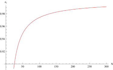
Figure 1 shows the increasing behavior of $n_{s}$ with respect to $N$. The observational value of $n_{s}=0.96$ corresponds to $N=60$ which indicates the physical compatibility of this anisotropic model with WMAP7 data. Equations (19) and (20) give the tensor power spectrum as well as spectral index, respectively as follows

$$\Delta^{2}_{T}(k) = \frac{2}{9\pi^{2}}(n+2)^{2}(\mu g)^{2}\left(\frac{\ln\mathcal{B}-\ln\mathcal{B}_{0}}{\omega_{0}}\right)^{\frac{16(g-1)}{5g+2}}$$

$$= \frac{2}{9\pi^{2}}(n+2)^{2}(\mu g)^{2}\left[\left(\frac{3}{n+2}\right)\left(\frac{N}{\mu}+\frac{1-g}{g\mu}\right)\right]^{\frac{2(g-1)}{g}},$$

$$n_{T} = -2\left(\frac{3}{n+2}\right)\left(\frac{1-g}{\mu g}\right)\left(\frac{\ln\mathcal{B}-\ln\mathcal{B}_{0}}{\omega_{0}}\right)^{\frac{-8g}{5g+2}}$$

$$= -\frac{6(1-g)}{(n+2)\mu g}\left[\left(\frac{3}{m+2}\right)\left(\frac{N}{\mu}+\frac{1-g}{g\mu}\right)\right]^{-1}.$$

The tensor-scalar ratio is obtained as

$$R = \left(\frac{48(4\pi)^{3}(n+2)^{4}(\mu g)^{4}}{\pi^{4}\eta^{3}_{0}}\right)^{\frac{1}{2}}\left[\frac{(2C_{\gamma})^{11}(1+2n)^{5}}{3^{11}(n+2)^{29}(\mu g)^{15}(1-g)^{3}}\right]^{\frac{1}{8}}$$

$$\times \mathcal{B}^{-3}\left(\frac{\ln\mathcal{B}-\ln\mathcal{B}_{0}}{\omega_{0}}\right)^{\frac{g+2}{5g+2}}$$

$$= \left(\frac{48(4\pi)^{3}(n+2)^{4}(\mu g)^{4}}{\pi^{4}\eta^{3}_{0}}\right)^{\frac{1}{2}}\left[\frac{(2C_{\gamma})^{11}(1+2n)^{5}}{3^{11}(n+2)^{29}(\mu g)^{15}(1-g)^{3}}\right]^{\frac{1}{8}}\mathcal{B}^{3}_{0}$$

$$\times \exp\left[3\omega_{0}\left(\left(\frac{3}{n+2}\right)\left(\frac{N}{\mu}+\frac{1-g}{g\mu}\right)\right)^{\frac{5g+2}{8g}}\right]$$

$$\times \left[\left(\frac{3}{n+2}\right)\left(\frac{N}{\mu}+\frac{1-g}{g\mu}\right)\right]^{\frac{g+2}{8g}}.$$

Rewriting the above equation in the form of $n_{s}$, we have

$$R = \left(\frac{48(4\pi)^{3}(n+2)^{4}(\mu g)^{4}}{\pi^{4}\eta^{3}_{0}}\right)^{\frac{1}{2}}\left[\frac{(2C_{\gamma})^{11}(1+2n)^{5}}{3^{11}(n+2)^{29}(\mu g)^{15}(1-g)^{3}}\right]^{\frac{1}{8}}\mathcal{B}^{3}_{0}$$ (30)

$$\times \exp\left[3\omega_{0}\left(\left(\frac{3}{n+2}\right)\left(\frac{18-15g}{8g\mu(1-n_{s})}\right)\right)^{\frac{5g+2}{8g}}\right]$$

$$\times \left[\left(\frac{3}{n+2}\right)\left(\frac{18-15g}{8g\mu(1-n_{s})}\right)\right]^{\frac{g+2}{8g}}.$$

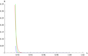
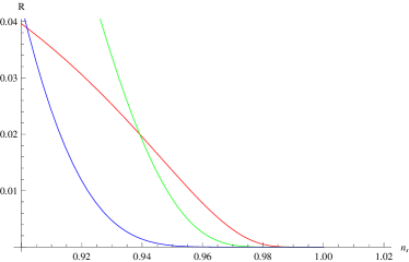
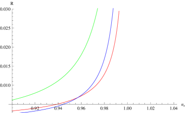
The left graph of Figure 2 shows that the anisotropic model is incompatible with WMAP7 data for all the three choices of dissipation factor. With the help of fine-tuning of the parameters $g$ and $\mu$, we are able to find the range $R<0.22$ in which $n_{s}=0.96$ lies for $\eta_{0}=0.25,~{}1,~{}4$. The compatible behavior of the tensor-scalar ratio with spectral index is shown in the right graph.

Figure 2: The left graph of scalar-tensor ratio versus $n_{s}$ for $\mu=1,~{}C_{\gamma}=70,~{}g=\frac{1}{2},~{}\mathcal{B}_{0}\propto C_{\gamma}^{-\frac{1}{12}},~{}n\approx 0.5,~{}\eta_{0}=0.25$(blue), $1$(green), $4$(red). The right graph is plotted for $\mu=5,~{}g=0.95$.

3.1.2 Case 2: $\eta=\eta_{1}=constant$

Now, we calculate all the above parameters by taking the constant dissipation factor. When $\eta$ is constant, $\mathcal{B}$ and $H_{2}$ take the following form

$$\mathcal{B}=\mathcal{B}_{0}+\omega_{1}t^{\frac{2g-1}{2}},\quad H_{2}=\mu g\left(\frac{\mathcal{B}-\mathcal{B}_{0}}{\omega_{1}}\right)^{\frac{2(g-1)}{2g-1}},$$ (31)

with $\omega_{1}=\left[\frac{8(1+2n)}{\eta_{1}(2g-1)^{2}}(1-g)(\mu g)^{2}\right]^{\frac{1}{2}}$. The corresponding slow-roll parameters are

$$\epsilon=(\frac{3}{n+2})\frac{1-g}{\mu g}\left(\frac{\mathcal{B}-\mathcal{B}_{0}}{\omega_{1}}\right)^{\frac{2g}{1-2g}},\quad\lambda=(\frac{3}{n+2})\frac{2-g}{\mu g}\left(\frac{\mathcal{B}-\mathcal{B}_{0}}{\omega_{1}}\right)^{\frac{2g}{1-2g}}.$$ (32)

In this case, the relationship between $\rho_{\gamma}$ and $\rho_{v}$ becomes

$$\rho_{\gamma}=\frac{9(1+2n)}{2(n+2)}(\mu g)(1-g)\left(\frac{\mathcal{B}-\mathcal{B}_{0}}{\omega_{1}}\right)^{\frac{4-2g}{1-2g}}.$$

The number of e-folds between $\mathcal{B}$ and $\mathcal{B}_{1}$ are calculated as

$$N=(\frac{m+2}{3})\mu\left[\left(\frac{\mathcal{B}-\mathcal{B}_{0}}{\omega_{1}}\right)^{\frac{2g}{2g-1}}-\left(\frac{\mathcal{B}_{1}-\mathcal{B}_{0}}{\omega_{1}}\right)^{\frac{2g}{2g-1}}\right],$$ (33)

where

$$\mathcal{B}_{1}=\mathcal{B}_{0}+\omega_{1}\left[\frac{3(1-g)}{(n+2)\mu g}\right]^{\frac{5g+2}{8g}}.$$

The scalar field in terms of e-folds is given as

$$\mathcal{B}=\mathcal{B}_{0}+\omega_{1}\left[\left(\frac{3}{n+2}\right)\left(\frac{N}{\mu}+\frac{1-g}{g\mu}\right)\right]^{\frac{2g-1}{2g}}.$$ (34)

Figure 3: The graph of $n_{s}$ versus number of e-folds.

The corresponding scalar power spectrum and spectral index are

$$\Delta^{2}_{R}(k) = \left[\left(\frac{3}{2C_{\gamma}}\right)^{\frac{1}{2}}\frac{(n+2)^{\frac{9}{2}}\eta^{3}_{1}(\mu g)^{\frac{3}{2}}}{972(4\pi)^{3}(1+2n)^{\frac{3}{2}}(1-g)^{\frac{3}{2}}}\right]^{\frac{1}{2}}$$ (35)

$$\times \left[\left(\frac{3}{n+2}\right)\left(\frac{N}{\mu}+\frac{1-g}{g\mu}\right)\right]^{\frac{3}{4}},$$

$$n_{s} = 1-\left(\frac{9}{4\mu(n+2)}\right)\left[\left(\frac{3}{n+2}\right)\left(\frac{N}{\mu}+\frac{1-g}{g\mu}\right)\right]^{-1}.$$

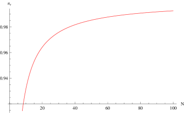
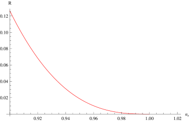
The graphical behavior of the spectral index against number of e-folds is shown in Figure 3. The corresponding number $N$ of $n_{s}=0.96$ decreases as compared to the previous case in which $\eta$ is a function of $\mathcal{B}$. In this case, the model remains consistent with WMAP7 observations. Similarly, $\Delta^{2}_{T}$ and $n_{T}$ can be written as

$$\Delta^{2}_{T} = \frac{2}{9\pi^{2}}(n+2)^{2}(\mu g)^{2}\left[\left(\frac{3}{n+2}\right)\left(\frac{N}{\mu}+\frac{1-g}{g\mu}\right)\right]^{\frac{2(g-1)}{g}},$$ (36)

$$n_{T} = -\frac{6(1-g)}{\mu g(m+2)}\left[\left(\frac{3}{n+2}\right)\left(\frac{N}{\mu}+\frac{1-g}{g\mu}\right)\right]^{-1}.$$

The tensor-scalar ratio can be found as

$$R = \left[\frac{48(4\pi)^{3}(1+2n)^{\frac{3}{2}}(\mu g)^{\frac{5}{2}}(1-g)^{\frac{3}{2}}(2C_{\gamma})^{\frac{1}{2}}}{\pi^{4}\eta^{3}_{1}3^{\frac{1}{2}}(n+2)^{\frac{1}{2}}}\right]^{\frac{1}{2}}$$

$$\times \left[\left(\frac{3}{n+2}\right)\left(\frac{N}{\mu}+\frac{1-g}{g\mu}\right)\right]^{\frac{5g-8}{4g}},$$

$$= \left[\frac{48(4\pi)^{3}(1+2n)^{\frac{3}{2}}(\mu g)^{\frac{5}{2}}(1-f)^{\frac{3}{2}}(2C_{\gamma})^{\frac{1}{2}}}{\pi^{4}\eta^{3}_{1}3^{\frac{1}{2}}(n+2)^{\frac{1}{2}}}\right]^{\frac{1}{2}}\left[\frac{4\mu(n+2)}{9}(1-n_{s})\right]^{\frac{8-5g}{4g}}.$$

Figure 4 shows the agreement of the considered model with WMAP data as the value of observational interest of $n_{s}$ lies in the region $R<0.22$.

Figure 4: The graph of scalar-tensor ratio versus $n_{s}$ for $\mu=1,~{}C_{\gamma}=70,~{}g=\frac{1}{2},~{}n\approx 0.5,~{}\eta_{1}\propto C_{\gamma}^{\frac{1}{6}}$.

3.2 Logamediate Inflation

Here we evaluate the above mentioned parameters in the context of logamediate inflation to study the dynamics of warm vector inflation. In this scenario, the scale factor has the specific form [14]

$$b(t)=b_{0}\exp(\mu[\ln t]^{\psi}),\quad\psi>1,~{}\mu>0.$$ (38)

Thus the number of e-folds is

$$N=\frac{(n+2)}{3}\mu([\ln t]^{\psi}-[\ln t_{1}]^{\psi}).$$ (39)

3.2.1 Case 1: $\eta=\eta_{0}\frac{T_{\gamma}^{3}}{\mathcal{B}^{2}}$

In this case, the scalar field and the directional Hubble parameter are

$$\mathcal{B} = \mathcal{B}_{0}\exp(\omega_{2}\Gamma(t)),$$ (40)

$$H_{2} = \mu\psi\left(\ln\left[\Gamma^{-1}\left(\frac{\ln\mathcal{B}-\ln\mathcal{B}_{0}}{\omega_{2}}\right)\right]\right)^{2(\psi-1)}\left[\Gamma^{-1}\left(\frac{\ln\mathcal{B}-\ln\mathcal{B}_{0}}{\omega_{2}}\right)\right]^{-2},$$

where $\omega_{2}=\left[\frac{2(2C_{\gamma})^{\frac{3}{4}}(\mu\psi)^{\frac{5}{4}}(n+2)^{\frac{3}{4}}(1+2n)^{\frac{1}{4}}}{3^{\frac{7}{4}}\eta_{0}}\right]^{\frac{1}{2}}$ and $\Gamma(t)=\gamma[\frac{5\psi+3}{8},\frac{\ln t}{4}]$ is the incomplete gamma function. The potential term is expressed in terms of $\mathcal{B}$ using Eqs.(9) and (40) as

$$V = \frac{2(1+2n)}{3}(\mu\psi)^{2}\left(\ln\left[\Gamma^{-1}\left(\frac{\ln\mathcal{B}-\ln\mathcal{B}_{0}}{\omega_{2}}\right)\right]\right)^{2(\psi-1)}$$ (42)

$$\times \left[\Gamma^{-1}\left(\frac{\ln\mathcal{B}-\ln\mathcal{B}_{0}}{\omega_{2}}\right)\right]^{-2}.$$

The slow-roll parameters can be described as

$$\epsilon = \frac{3}{(n+2)\mu\psi}\left(\ln\left[\Gamma^{-1}\left(\frac{\ln\mathcal{B}-\ln\mathcal{B}_{0}}{\omega_{2}}\right)\right]\right)^{2(\psi-1)},$$

$$\lambda = \frac{6}{(n+2)\mu\psi}\left(\ln\left[\Gamma^{-1}\left(\frac{\ln\mathcal{B}-\ln\mathcal{B}_{0}}{\omega_{2}}\right)\right]\right)^{2(\psi-1)}.$$ (43)

The corresponding energy density of radiation is

$$\rho_{\gamma} = \frac{9(1+2n)}{2(m+2)}(\mu\psi)\left(\ln\left[\Gamma^{-1}\left(\frac{\ln\mathcal{B}-\ln\mathcal{B}_{0}}{\omega_{2}}\right)\right]\right)^{6(\psi-1)}$$

$$\times \left(\Gamma^{-1}\left(\frac{\ln\mathcal{B}-\ln\mathcal{B}_{0}}{\omega_{2}}\right]\right)^{-4}.$$

The number of e-folds between two fields is given as

$$N=\left(\frac{n+2}{3}\right)\mu\left[\left(\ln\left[\Gamma^{-1}\left(\frac{\ln\mathcal{B}-\ln\mathcal{B}_{0}}{\omega_{2}}\right)\right]\right)^{\psi}-\left(\frac{(n+2)}{3}\mu\psi\right)^{\frac{\psi}{1-\psi}}\right].$$ (44)

The second equality in the above equation is obtained by using the value of $\mathcal{B}_{1}$ and putting $\epsilon=1$. Equation (40) can be rewritten in terms of e-folds as

$$\mathcal{B}=\mathcal{B}_{0}\exp\left[\omega_{2}\Gamma\exp\left[\left(\frac{3}{n+2}\right)\frac{N}{\mu}+\left(\frac{3}{n+2}\mu\psi\right)^{\frac{\psi}{1-\psi}}\right]^{\frac{1}{\psi}}\right].$$ (45)

The corresponding perturbed parameters $\Delta^{2}_{R}(k)$ and $\Delta^{2}_{T}(k)$ are

$$\Delta^{2}_{R}(k) = \left(\frac{\eta^{3}_{0}}{(4\pi)^{3}}\right)^{\frac{1}{2}}\left[\frac{3^{11}(m+2)^{9}(\mu\psi)^{15}(1+2n)^{3}}{(2C_{\gamma})^{11}}\right]^{\frac{1}{8}}\mathcal{B}^{-3}_{0}$$ (46)

$$\times \exp\left[-3\omega_{2}\Gamma\exp\left[\left(\frac{3}{n+2}\right)\frac{N}{\mu}+\left(\frac{3}{n+2}(\mu\psi)\right)^{\frac{\psi}{1-\psi}}\right]^{\frac{1}{\psi}}\right]$$

$$\times \exp\left[\frac{-15}{8}\left(\exp\left[\left(\frac{3}{n+2}\right)\frac{N}{\mu}+\left(\frac{3}{n+2}(\mu\psi)\right)^{\frac{\psi}{1-\psi}}\right]^{\frac{1}{\psi}}\right)\right]$$

$$\times \left[\left(\frac{3}{n+2}\right)\frac{N}{\mu}+\left(\frac{3}{n+2}(\mu\psi)\right)^{\frac{\psi}{1-\psi}}\right]^{\frac{15(\psi-1)}{8\psi}},$$

$$\Delta^{2}_{T} = \frac{2}{9\pi^{2}}(m+2)^{2}(\mu\psi)^{2}\left[\left(\frac{3}{n+2}\right)\frac{N}{\mu}+\left(\frac{3}{n+2}(\mu\psi)\right)^{\frac{\psi}{1-\psi}}\right]^{\frac{2(\psi-1)}{\psi}}$$ (47)

$$\times \exp\left[-2\left(\left(\frac{3}{n+2}\right)\frac{N}{\mu}+\left(\frac{3}{n+2}(\mu\psi)\right)^{\frac{\psi}{1-\psi}}\right)^{\frac{1}{\psi}}\right].$$

The corresponding spectral indices are

$$n_{s}-1 = \frac{15(1-\psi)}{8\mu\psi}\left(\frac{3}{n+2}\right)\left[\left(\frac{3}{n+2}\right)\frac{N}{\mu}+\left(\frac{3}{n+2}(\mu\psi)\right)^{\frac{\psi}{1-\psi}}\right]^{-1},$$

$$n_{T} = -\frac{6}{(n+2)\mu\psi}\left[\left(\frac{3}{n+2}\right)\frac{N}{\mu}+\left(\frac{3}{n+2}(\mu\psi)\right)^{\frac{\psi}{1-\psi}}\right]^{1-\psi}.$$

Figure 5: The graph of $n_{s}$ versus number of e-folds for $\mu=1,~{}\psi=10$(red), $50$(blue), $n\approx 0.5$ in logamediate scenario.

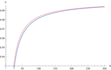
Figure 5 indicates the behavior of $n_{s}$ against $N$ for $\psi=10,~{}50$. The number of e-folds decreases as $\psi$ increases. Here the allowed value of the parameter $n_{s}=0.96$ lies in the range $N\approx 50$. Finally, we obtain the following observational parameter of interest as a function of spectral index

$$R = \left(\frac{4(4\pi)^{3}}{81\pi^{4}\eta^{3}_{0}}\right)^{\frac{1}{2}}\left[\frac{(2C_{\gamma})^{11}(n+2)^{7}(\mu\psi)}{3^{11}(1+2n)^{3}}\right]^{\frac{1}{8}}\mathcal{B}^{3}_{0}\left[\left(\frac{3}{n+2}\right)\frac{15(\psi-1)}{8\mu\psi(1-n_{s})}\right]^{\frac{1}{\psi}}$$ (49)

$$\times \exp\left[3\omega_{2}\Gamma\exp\left[\left(\frac{3}{n+2}\right)\frac{15(\psi-1)}{8\mu\psi(1-n_{s})}\right]^{\frac{1}{\psi}}\right]$$

$$\times \exp\left[-\frac{1}{8}\left[\left(\frac{3}{n+2}\right)\frac{15(\psi-1)}{8\mu\psi(1-n_{s})}\right]^{\frac{1}{\psi}}\right].$$

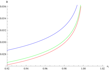
We see from Figure 6 the consistency of the model with observational data for specific values of $\eta_{0}$. The ratio $R$ decreases as $\psi$ increases.

Figure 6: The left graph of scalar-tensor ratio versus $n_{s}$ for $\mu=1,~{}C_{\gamma}=70,~{}f=\frac{1}{2},~{}n\approx 0.5,~{}\mathcal{B}_{0}\propto C_{\gamma}^{-\frac{1}{12}},~{}\psi=10,~{}\eta_{0}=0.25$(blue), $1$(green), $4$(red). The right graph is plotted for $\psi=50$.

3.3 Case 2: $\eta=\eta_{1}$

For this case, the scalar field and the directional Hubble parameter are

$$\mathcal{B}=\mathcal{B}_{0}+\omega_{3}\Gamma(t),\quad H_{2}=\frac{\mu\psi\left(\ln\left[\Gamma^{-1}\left(\frac{\mathcal{B}-\mathcal{B}_{0}}{{\omega}_{3}}\right)\right]\right)^{(\psi-1)}}{\Gamma^{-1}\left(\frac{\mathcal{B}-\mathcal{B}_{0}}{{\omega}_{3}}\right)},$$ (50)

where ${\omega}_{3}=\left[\frac{2(1+2n)(\mu\psi)^{2}}{\eta_{1}}\right]^{\frac{1}{2}}\frac{(\psi-1)!}{2^{\psi-1}}$ and $\Gamma(t)=\gamma[\psi,\frac{\ln t}{2}]$. In this case, $V$ transformed into

$$V=\frac{2(1+2n)}{3}\left[\frac{(\mu\psi)\left(\ln\left[\Gamma^{-1}\left(\frac{\mathcal{B}-\mathcal{B}_{0}}{\omega_{3}}\right)\right]\right)^{(\psi-1)}}{{\Gamma^{-1}\left(\frac{\mathcal{B}-\mathcal{B}_{0}}{\omega_{3}}\right)}}\right]^{2}.$$

The parameters $\epsilon$ and $\lambda$ take the following form

$$\epsilon=\frac{3\left(\ln\left[\Gamma^{-1}\left(\frac{\mathcal{B}-\mathcal{B}_{0}}{\omega_{3}}\right)\right]\right)^{1-\psi}}{(n+2)(\mu\psi)},\quad\lambda=\frac{6\left(\ln\left[\Gamma^{-1}\left(\frac{\mathcal{B}-\mathcal{B}_{0}}{\omega_{3}}\right)\right]\right)^{1-\psi}}{(n+2)(\mu\psi)}.$$ (51)

The number of e-folds becomes

$$N=\left(\frac{n+2}{3}\right)\mu\left[\left(\ln\left[\Gamma^{-1}\left(\frac{\mathcal{B}-\mathcal{B}_{0}}{\omega_{3}}\right)\right]\right)^{\psi}-\left[\frac{n+2}{3}(\mu\psi)\right]^{\frac{\psi}{1-\psi}}\right].$$ (52)

The scalar field is

$$\mathcal{B}=\mathcal{B}_{0}+\omega_{3}\Gamma\exp\left[\left(\frac{3}{n+2}\right)\frac{N}{\mu}+\left(\frac{n+2}{3}(\mu\psi)\right)^{\frac{\psi}{1-\psi}}\right]^{\frac{1}{\psi}}.$$ (53)

The power spectrums in scalar and tensor forms can be found as

$$\Delta^{2}_{R}(k) = \left(\frac{\eta^{3}_{1}(n+2)^{\frac{9}{2}}3^{\frac{1}{2}}(\mu\psi)^{\frac{3}{2}}}{972(1+2n)^{\frac{3}{2}}(4\pi)^{3}(2C_{\gamma})^{\frac{1}{2}}}\right)^{\frac{1}{2}}\left[\left(\frac{3}{n+2}\right)\frac{N}{\mu}\right.$$

$$+ \left.\left(\frac{n+2}{3}(\mu\psi)\right)^{\frac{\psi}{1-\psi}}\right]^{\frac{3(\psi-1)}{4\psi}},$$

$$\Delta^{2}_{T}(k) = \frac{2(1+2n)}{3\pi^{2}}(\mu\psi)^{2}\left[\left(\frac{3}{n+2}\right)\frac{N}{\mu}+\left(\frac{3}{n+2}(\mu\psi)\right)^{\frac{\psi}{1-\psi}}\right]^{\frac{2(\psi-1)}{\psi}}$$ (54)

$$\times \exp\left[-2\left(\left(\frac{3}{n+2}\right)\frac{N}{\mu}+\left(\frac{3}{n+2}(\mu\psi)\right)^{\frac{\psi}{1-\psi}}\right)^{\frac{1}{\psi}}\right].$$

The terms $n_{s}$ and $n_{T}$ related to the above equations become

$$n_{s}-1 = \frac{9(1-\psi)}{4\mu\psi(n+2)}\left[\left(\frac{3}{n+2}\right)\frac{N}{\mu}+\left(\frac{n+2}{3}(\mu\psi)\right)^{\frac{\psi}{1-\psi}}\right]^{-1},$$ (55)

$$n_{T} = -\frac{6}{(n+2)\mu\psi}\left[\left(\frac{3}{n+2}\right)\frac{N}{\mu}+\left(\frac{n+2}{3}(\mu\psi)\right)^{\frac{\psi}{1-\psi}}\right]^{\frac{1-\psi}{\psi}}.$$

Figure 7 shows similar behavior as for the large values of $\psi$ gives small values of the $N$. The value $N\approx 20$ coincides with $n_{s}=0.96$ and verifies the compatibility of this case with observational data. Curves for $\psi=50$ and $\psi=70$ overlap each other in the allowed range. Consequently, $R$ can be represented as

$$R = \left(\frac{3888(1+2n)^{\frac{7}{2}}(4\pi)^{3}(2C_{\gamma})^{\frac{1}{2}}(\mu\psi)^{\frac{5}{2}}}{81\pi^{4}\eta^{3}_{1}(n+2)^{\frac{9}{2}}3^{\frac{5}{2}}}\right)^{\frac{1}{2}}\left[\left(\frac{3}{n+2}\right)\frac{3(\psi-1)}{4\mu\psi(1-n_{s})}\right]^{\frac{5(\psi-1)}{4\psi}}$$ (56)

$$\times \exp\left[-2\left(\left(\frac{3}{n+2}\right)\frac{3(\psi-1)}{4\mu\psi(1-n_{s})}\right)^{\frac{1}{\psi}}\right].$$

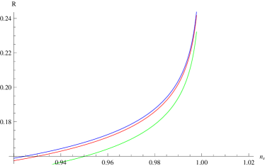
Figure 8 verifies the compatibility of the anisotropic BI universe model in the constant logamediate inflation regime with WMAP7 data.

Figure 7: The graph of $n_{s}$ versus number of e-folds for $\mu=1,~{}\psi=10$(red), $50$(green), $70$(blue), $n\approx 0.5$.

Figure 8: The graph of scalar-tensor ratio versus $n_{s}$ for $\mu=1,~{}C_{\gamma}=70,~{}\psi=10$(red), $50$(green), $70$(blue), $n\approx 0.5,~{}\eta_{1}\propto C_{\gamma}^{\frac{1}{6}}$.

4 Concluding Remarks

It is well-known that inflation due to scalar fields is compatible with completely isotropic universe. In this paper, we assume vector field inflation which can provide the isotropic (by orthogonal triplet vector fields) as well as anisotropic universe (with randomly oriented $N$ vector fields). The anisotropic fields can be achieved in two ways, i.e., by applying initial conditions on the potential and fine-tuning of the inflationary time period. The anisotropy is of the order $1/\sqrt{N}$ at the end of inflation. We have investigated the role of warm vector inflation in the framework of LRS BI universe model. A triplet of mutually orthogonal vectors is introduced to remove the off-diagonal terms from the components of the energy-momentum tensor as the considered model is symmetric. We construct the field equations and conservation equations under the slow-roll approximation using a specific form of the dissipation coefficient. We have assumed the dissipation of the inflation density into radiation density $(\eta>0)$.

The slow-roll parameters $(\epsilon,\lambda)$ are presented in the context of anisotropic warm vector inflation. Using these parameters and applying strong dissipative regime, we have calculated the more general conditions for the starting and ending of the inflationary era (13). In warm inflation, thermal fluctuations are produced instead of quantum fluctuations which are characterized by power spectra $(\Delta^{2}_{R}(k),\Delta^{2}_{T}(k))$ and spectral indices $(n_{S},n_{T})$. We have evaluated all these perturbed parameters under slow-roll conditions and finally an important parameter, i.e., tensor-scalar ratio which is constrained by WMAP7 observations.

We have developed our model in intermediate and logamediate models as they represent exact cosmological solutions. Each era is discussed for two possible choices of $\eta$, i.e., it is a function of scalar field and some positive constant. The directional Hubble parameter, slow-roll as well as perturbation parameters are calculated in these frameworks of inflation for anisotropic universe. According to the observations of WMAP7, the best fit values of these parameters $(\Delta^{2}_{R}(k),n_{S},R)$ have been calculated with higher degree of accuracy. We have checked the physical compatibility of our model with the results of WMAP7, i.e., the standard value $n_{S}=0.96$ must be found in the region $R<0.22$. The behavior of these parameters are checked through graphs of $N$ and $R$ versus $n_{S}$ in each case.

During intermediate scenario with variable $\eta$, we have seen that $n_{S}=0.96$ corresponds to $N=50$. The left $R-n_{S}$ trajectories in Figure 2 shows the inconsistency of the model with WMAP7 for $\mu=1,~{}C_{\gamma}=70,~{}g=\frac{1}{2},~{}\mathcal{B}_{0}\propto C_{\gamma}^{-\frac{1}{12}},~{}n\approx 0.5,~{}\eta_{0}=0.25,~{}1,~{}4$. The method of fine-tuning helps to find the allowed range and hence $n_{S}=0.96$ is located in the region $R<0.22$ for $\mu=5,~{}g=\frac{1}{2},~{}\mathcal{B}_{0}\propto C_{\gamma}^{-\frac{1}{12}},~{}n\approx 0.5,~{}\eta_{0}=0.25,~{}1,~{}4$. The isotropic universe [17] for this case is compatible with WMAP7 only for $\eta_{0}=1$ keeping the same rest of the parameters. For constant $\eta$, the model remains compatible with observational data. Hence the anisotropic universe model is compatible with WMAP7 data during variable and constant intermediate inflation. Figures 5-8 indicate the compatibility of the variable as well as constant logamediate inflationary scenario in the framework of anisotropic universe with WMAP7 data. We would like to mention here that this model is consistent for all chosen values of $\psi$ and $\eta_{0}$ while isotropic universe for variable dissipation factor is compatible only for $\eta_{0}=1$. We have also observed that the compatibility of the model disturbs for large values of the anisotropic parameter $(n)$. It is interesting that all the results reduce to the isotropic universe (FRW) for $n=1$.

References

- [1] Perlmutter, S. et al.: Astron. Soc. 29(1997)1351; Nature 391(1998)51; Riess, A.G. et al.: Astron. J. 116(1998)1009; Bennett, C.L. et al.: Astrophys. J. Suppl. 148(2003)1; Peebles, P.J.E. and Ratra, B.: Rev. Mod. Phys. 75(2003)559; Tegmark, M. et al.: Phys. Rev. D 69(2004)03501; Spergel, D.N. et al.: Astrophys. J. Suppl. 170(2007)377.
- [2] Darabi, F.: arXiv:1107.3307.
- [3] Ratra, B. and Peebles, P.J.E.: Phys. Rev. D 37(1998)3406; Chiba, T., Okabe, T. and Yamaguchi, M.: Phys. Rev. D 62(2000)023511; Sen, A.: J. High Energy Phys. 48(2002)204; Padmanabhan, T.: Phys. Rev. D 66(2002)021301; Guo, Z.K. et al.: Phys. Lett. B 608(2005)177; Padmanabhan, T.: Gen. Relativ. Gravit. 40(2008)529.
- [4] Gorini, V., Kamenshchik, A. and Moschella, U.: Phys. Rev. D 67(2003)063509; Wang, B., Gong, Y.G. and Abdalla, E.: Phys. Lett. B 624(2005)141; Hu, B. and Ling, Y.: Phys. Rev. D 73(2006)123510; Setare, M.R.: J. of Cosmology and Astrophys. 0701(2007)023.
- [5] Guth, A.: Phys. Rev. D 23(1981)347; Albrecht, A. and Steinhardt, P. J.: Phys. Rev. Lett. 48(1982)1220.
- [6] Gold, B. et al.: arXiv:1001.4555; Komatsu, E. et al.: Astrophys. J. Suppl. 192(2011)18; Larson, D. et al.: Astrophys. J. Suppl. 192(2011)16.
- [7] Golovnev, A., Mukhanov, V. and Vanchurin, V.: J. Cosmol. Astropart. Phys. 0806(2008)009.
- [8] Bardeen, J.M., Steinhardt, P.J. and Turner, M.S.: Phys. Rev. D 28(1983)679; Linde, A.: Phys. Lett. B 129(1983)177; Kolb, E.W. and Turner, M.S.: The Early Universe, (Addison-Wesley, New York, 1990).
- [9] Bassett, B.A., Tsujikawa, S. and Wands, D.: Rev. Mod. Phys. 78(2006)537.
- [10] Berera, A.: Phys. Rev. Lett. 75(1995)3218; Phys. Rev. D 55(1997)3346.
- [11] Moss, I.G.: Phys. Lett. B 154(1985)120; Berera, A.: Nucl. Phys. B 585(2000)666; Hall, L.M.H., Moss, I.G. and Berera, A.: Phys. Rev. D 69(2004)083525.
- [12] Sanyal, A.K.: Phys. Lett. B 645(2007)1.
- [13] Yokoyama, J. and Maeda, K.: Phys. Lett. B 207(1988)31.
- [14] Barrow, J.D.: Class. Quantum Grav. 13(1996)2965.
- [15] Barrow, J.D.: Phys. Rev. D 51(1995)2729 .
- [16] Ferreira, P.G. and Joyce, M.: Phys. Rev. D 58(1998)023503; Peebles, P.J.E. and Ratra, B.: Rev. Mod. Phys. 75(2003)559; Barrow, J.D. and Nunes, N.J.: Phys. Rev. D 76(2007)043501.
- [17] Setare, M.R. and Kamali, V.: arXiv:1309.2452.
- [18] Collins, C.B.: Phys. Lett. A 60(1977)397; Sharif, M. and Zubair, M.: Astrophys. Space Sci. 330(2010)399.
- [19] Armendariz-Picon, C.: J. Cosmol. Astropart. Phys. 07(2004)007.
- [20] Mukhanov, V.: Physical Foundations of Cosmology (Cambridge University Press, 2005).
- [21] Bastero-Gil, M., Berera, A. and Ramos, R.O.: J. Cosmol. Astropat. Phys. 1109(2011)033; Bastero-Gil, M., Berera, A., Ramos, R.O. and Rosa, J.G.: J. Cosmol. Astropart. Phys. 1301(2013)016.
- [22] Hwang, J.C. and Noh, H.: Phys. Rev. D 66(2002)084009.
- [23] Guth, A.H. and Pi, S.Y.: Phys. Rev. Lett. 49(1982)1110; Hawking, S.W.: Phys. Lett. B 115(1982)295; Starobinsky, A.A.: Phys. Lett. B 117(1982)175; Bardeen, J.M., Steinhardt, P.J. and Turner, M.S.: Phys. Rev. D 28(1983)679.
- [24] Freese, K., Frieman, J.A. and Olinto, A.V.: Phys. Rev. Lett. 65(1990)3233.