Universal scaling of Lyapunov-exponent fluctuations in space-time chaos

Abstract

Finite-time Lyapunov exponents of generic chaotic dynamical systems fluctuate in time. These fluctuations are due to the different degree of stability across the accessible phase-space. A recent numerical study of spatially-extended systems has revealed that the diffusion coefficient $D$ of the Lyapunov exponents (LEs) exhibits a non-trivial scaling behavior, $D(L)\sim L^{-\gamma}$, with the system size $L$. Here, we show that the wandering exponent $\gamma$ can be expressed in terms of the roughening exponents associated with the corresponding “Lyapunov-surface”. Our theoretical predictions are supported by the numerical analysis of several spatially-extended systems. In particular, we find that the wandering exponent of the first LE is universal: in view of the known relationship with the Kardar-Parisi-Zhang equation, $\gamma$ can be expressed in terms of known critical exponents. Furthermore, our simulations reveal that the bulk of the spectrum exhibits a clearly different behavior and suggest that it belongs to a possibly unique universality class, which has, however, yet to be identified.

I Introduction

Lyapunov exponents (LEs) $\langle\lambda_{i}\rangle$ are the most powerful tool for a detailed characterization of chaotic dynamics ott : they allow determining the number of unstable directions, the Kolmogorov-Sinai entropy, the fractal dimension and other dynamical invariants. The number of LEs equals the number of degrees of freedom $N$. The LEs, ordered from the largest to the smallest one, define the so-called spectrum of LEs. In spatially extended systems, $N\propto L^{d}$ (where $L$ is the system linear size and $d$ is the dimensionality of the space); in the thermodynamic limit ($L\to\infty$) the Lyapunov spectrum converges to an asymptotic curve, that is specific to each system and depends only on $\rho=i/L^{d}$. The existence of such a limit shape is taken as the proof of extensivity, i.e. that quantities like the fractal dimension or the Kolmogorov–Sinai entropy are proportional to the system volume.

The LEs quantify the exponential expansion (contraction) growth rates along the $N$ covariant or characteristic directions in the infinite-time limit. In fact, tangent space can be decomposed into covariant subspaces and the corresponding vector-base provides relevant information that is encoded in the so-called characteristic/covariant Lyapunov vectors (LVs) ruelle79 ; eckmann ; legras96 . These vectors actually contribute to identify the local structure of the invariant measure, to uncover the possible presence of collective phenomena takeuchi09 , to determine the dimension of the inertial manifold yang09 , or to detect spurious LEs observed in embedded time series yang12 , to cite a few applications.

In a time interval $t$, an infinitesimal perturbation pointing along the $i$-th LV is expanded/contracted in tangent space by a factor $e^{\Lambda_{i}(t)}$, where $\Lambda_{i}(t)$ is the so-called expansion rate. As a result of the variable degree of instability in phase-space, $\Lambda_{i}(t)$ fluctuates along the trajectory (or, equivalently, across phase-space). Nevertheless, the finite-time Lyapunov exponent (FTLE) $\lambda_{i}(t)=\Lambda_{i}(t)/t$ converges, in the infinite-time limit, to the $i$-th LE, $\lim_{t\to\infty}\lambda_{i}(t)=\langle\lambda_{i}\rangle$, where brackets indicate an average over trajectories foot1 (hereafter, phase-space average and time average are assumed to coincide).

It is natural to ask how the FTLE fluctuations scale with both time and system size. As already argued in kuptsov11 , this question is not only connected with the convergence to the thermodynamic limit, but also with the extensivity of space-time chaos. The best way to approach the problem is by introducing the (time-dependent) variances,

$$\chi^{2}_{ij}=\langle{\Lambda_{i}(t)\Lambda_{j}(t)}\rangle-\langle\lambda_{i}\rangle\langle\lambda_{j}\rangle t^{2}\,,$$ (1)

and the corresponding diffusion coefficients,

$$D_{ij}=\lim_{t\to\infty}\frac{\chi^{2}_{ij}}{t}\,.$$ (2)

It is expected that for large-enough times, the distribution ${\cal P}({\bm{\lambda}},t)$ of FTLEs [$\bm{\lambda}(t)=(\lambda_{1}(t),\dots,\lambda_{N}(t))$] is described by a suitable large-deviation function, ${\cal P}({\bm{\lambda}},t)\propto\exp[-S({\bm{\lambda}})t]$, and $S(\langle\bm{\lambda}\rangle)=0$. Under the fairly general assumption that the LEs fluctuations are short-range in time, (this is typically true away from bifurcations and phase transitions), the central limit theorem implies that $S(\bm{\lambda})$ has a quadratic structure around its minimum, i.e. that ${\cal P}({\bm{\lambda}},t)$ is Gaussian,

$${\cal P}({\bm{\lambda}},t)\propto\exp\left[-\frac{t}{2}({\bm{\lambda}}-\langle{\bm{\lambda}}\rangle)\mathrm{\mathbf{Q}}({\bm{\lambda}}-\langle{\bm{\lambda}}\rangle)^{\dagger}\right]\,,$$ (3)

where ${\dagger}$ denotes the transpose, while the matrix $\mathbf{Q}$ is the inverse of the symmetric diffusion matrix, i.e., $\mathbf{Q}=\mathbf{D}^{-1}$. Thus, within the Gaussian approximation, $\mathbf{D}$ describes how strong FTLE fluctuations are for a given system size. In particular, the diagonal elements $D_{ii}$ correspond to the diffusion coefficient of the expansion rates $\Lambda_{i}$ around the average growth $\langle\lambda_{i}\rangle t$.

Chaos extensivity would naively suggest that the diffusion coefficients should scale as $L^{-d}$ with the system size. Based on the numerical simulation of a variety of systems in $d=1$ Kuptsov and Politi kuptsov11 , have however found that $D_{ii}(L)\sim L^{-\gamma}$ with a wandering exponent that is smaller than 1: $\gamma\simeq 0.85$ for $i>1$, while $\gamma=1/2$ for $i=1$. At the same time, it was found that the off-diagonal terms decay as $L^{-1}$ and so do the eigenvalues of the matrix $\mathbf{D}$, in agreement with the expectation for an extensive chaotic dynamics. It is rather intriguing that although the matrix $\mathbf{D}$ becomes increasingly diagonal in the thermodynamic limit, its diagonal terms scale differently from the matrix eigenvalues kuptsov11 . In the absence of theoretical arguments, one cannot a priori exclude that the scaling behavior of the bulk of the spectrum is affected by strong finite-size corrections, so that $\gamma\to 1$ as $L\to\infty$. We shed some light on this problem by resorting to the well-known connection between LV dynamics and the kinetics of rough surfaces. This allows unveiling a theoretical connection between the scaling properties of the FTLEs fluctuations and the velocity fluctuations of rough surfaces subject to stochastic forces. This mapping leads to a scaling relation between the universal roughening exponents and the FTLE wandering exponent $\gamma$, which thus turns out to be a true critical exponent.

More specifically, in Section II, we develop the theoretical scaling arguments which lead us to derive the relevant mathematical relationships. In Section III, our systematic investigation of the maximal Lyapunov exponent confirms the theoretical expectations as well as the relationship with Kardar-Parisi-Zhang (KPZ) dynamics kpz . Section IV is devoted to the entirely new analysis of the bulk of the spectrum which suggests the correspondence with some yet unknown stochastic field theory. Finally, in Section V, we summarize the main results and briefly discuss the open problems.

II Theory

In this section we focus on the scaling behavior of the diagonal elements $D_{ii}$ of the matrix $\mathbf{D}$. For the sake of simplicity, from now on, we drop the index $i$ in the formulas and reintroduce it in the next sections, when it will be necessary to distinguish between different values of the integrated density $\rho=i/L^{d}$.

In the following we show that $D(L)\sim L^{-\gamma}$, where the exponent $\gamma$ can be expressed in terms of the scaling properties of the corresponding LV, $v(\bm{x},t)$. Our scaling theory is based upon the well-known interpretation of the dynamics of a LV as the statistical evolution of a rough surface pik94 ; pik98 ; pik01 ; szendro07 ; pazo08 .

For each given LV $v({\bm{x}},t)$ we define an associated “surface” field $h({\bm{x}},t)$ through the logarithmic transformation $h({\bm{x}},t)=\ln|v({\bm{x}},t)|$. The LV surface so defined is known to be generically rough and scale-invariant pik94 ; pik98 ; pik01 ; szendro07 ; pazo08 . As we are interested in the expansion factor of the LV over a time interval $t$, it is useful to introduce the field

$$\phi({\bm{x}},t)=h({\bm{x}},t)-h({\bm{x}},0)\,,$$ (4)

which corresponds to the logarithm of the finite-time expansion factor (over a time $t$). The fluctuations around the average surface position at any given time are quantified by the surface width $W$,

$$W^{2}(t,L)=\left\langle\overline{\phi^{2}({\bm{x}},t)}\right\rangle-\left\langle\overline{\phi({\bm{x}},t)}^{2}\right\rangle\,,$$ (5)

where the angular brackets denote an average over an ensemble of different trajectories, while the overline is a spatial average (here and in the following). Scale invariance generically leads to finite-size scaling of surface fluctuations that can be cast in the typical scaling form Barabasi

$$W^{2}(t,L)=L^{2\alpha}\mathcal{F}(t/L^{z})$$ (6)

where $\mathcal{F}(u)$ is a dynamical scaling function, which reaches asymptotically ($u\to\infty$) a constant value and grows as $u^{2\alpha/z}$ for small values of $u$. All of the above means that at short times $W^{2}$ grows as $t^{2\alpha/z}$, until $t\sim L^{z}$ when $W^{2}$ saturates to a size-dependent value $L^{2\alpha}$. The roughness exponent $\alpha$ and the dynamic exponent $z$ quantify space-time correlations and fully characterize the statistical and dynamical behavior of the surface (equivalently, the LV.)

II.1 Main result

Before proceeding with the details of the theoretical derivation, we anticipate our main result, i.e. that for any FTLE its variance $\chi^{2}(t,L)$ [defined by (1) with $i=j$] scales as

$$\chi^{2}(t,L)=L^{2\alpha-z}\mathcal{G}(t/L^{z})t\,.$$ (7)

where $\mathcal{G}(u\gg 1)\simeq\mathrm{const}$. By then comparing this formula with Eq. (2), this implies that the LE diffusion coefficient scales as

$$D(L)=L^{2\alpha-z}\mathcal{G}(\infty)\,,$$ (8)

so that the wandering exponent $\gamma$ heuristically observed in Ref. kuptsov11 is a truly critical exponent, connected to the LV surface roughening exponents,

$$\gamma=z-2\alpha\,.$$ (9)

As a result, $\gamma$ can be determined, once the roughening exponents of the corresponding surfaces are known. This is valid for any spatial dimension $d$.

II.2 Derivation of the scaling function $\cal G$

We now derive Eq. (8) and give further details on the scaling of the diagonal elements of $\mathbf{D}$ in the intermediate regime before saturation. First, let us notice that the expansion rate $\Lambda(t)$ necessarily refers to some norm in tangent space. The norm selection is irrelevant for the calculation of dynamical invariant quantities like the LEs or the diffusion coefficient $\mathbf{D}$, as they involve an infinite-time limit. However, the finite-time expansion rates $\Lambda(t)$ depend explicitly on the norm. Given a perturbation $v({\bm{x}},t)$, a rather broad family of $q$-norms can be defined as follows

$$\|v({\bm{x}},t)\|_{q}\equiv\left[(1/L)^{d}\sum_{\bm{x}}\left|v({\bm{x}},t)\right|^{q}\right]^{1/q}.$$ (10)

The standard Euclidean norm corresponds to $q=2$. In the following, our theoretical arguments will be developed with reference to the 0-norm: $\|v({\bm{x}},t)\|_{0}=\prod_{\bm{x}}\left|v({\bm{x}},t)\right|^{1/L^{d}}$, unless otherwise specified. The 0-norm is the most convenient and natural choice because, in this framework, computing the LV norm corresponds to determining the average height of the surface $h({\bm{x}},t)=\ln|v({\bm{x}},t)|$, while the FTLE corresponds to the surface velocity, so that

$$\Lambda(t)=\overline{\phi({\bm{x}},t)}\,,$$ (11)

which, by definition (4), corresponds to the net displacement of the average surface position in a time interval $t$.

Now, by combining Eqs. (1) and (11) one obtains

$$\chi^{2}(t,L)=\left\langle\overline{\phi({\bm{x}},t)}^{2}\right\rangle-\left\langle\overline{\phi({\bm{x}},t)}\right\rangle^{2}\,.$$ (12)

This expression, like Eq. (5) for $W^{2}$, is a quadratic correlation function of $\phi({\bm{x}},t)$ and, therefore, it should scale as

$$\chi^{2}(t,L)=L^{2\alpha}\mathcal{G}_{\chi}(t/L^{z})\,.$$ (13)

Consistency with Eq. (2) requires that $\mathcal{G}_{\chi}(u)$ diverges linearly with time. This information can be included in the above equation, by writing the scaling function as a product, $\mathcal{G}_{\chi}(u)=\mathcal{G}(u)u$, where $\mathcal{G}$ saturates for $u\to\infty$. Altogether, this leads to Eq. (7) and the main relation (9) for the scaling behavior of the asymptotic diffusion coefficient.

Although our theoretical arguments are based on the use of the 0-norm, this does not affect the validity of our main scaling relation (9) as, in the infinite-time limit, the diffusion coefficient $D$ is actually a dynamical invariant, independent of the norm used.

Before saturation sets in ($t\ll L^{z}$), the effective diffusion coefficient is time-dependent and exhibits long-range temporal correlations. These correlations are important, since they correspond to an anomalous diffusion of the expansion rate $\Lambda$, as it can be inferred by looking at the “short-time” behavior of the dynamic scaling function $\mathcal{G}$ in Eq. (7), i.e. for $1\ll t\ll L^{z}$. We indeed find that, still in the 0-norm framework,

$$\mathcal{G}(u)\approx u^{\nu}\,\,\mbox{with}\,\,\nu=\frac{2\alpha-z+d}{z}\,.$$ (14)

Let us now show how this result arises from a simple scaling argument. At short times, correlations only extend over a linear distance of order $\sim t^{1/z}$ so that the system can be considered as formed by a number $N_{b}\sim(L/t^{1/z})^{d}$ of statistically independent blocks. Accordingly, we can write $\phi({\bm{x}},t)=\left\langle\,\overline{\phi}\,\right\rangle+\delta\phi({\bm{x}},t)$, where $\delta\phi({\bm{x}},t)$ is the local (intra-block) fluctuation. From Eq. (12), we can now estimate $\chi^{2}$

$$\chi^{2}=\left\langle\overline{\phi({\bm{x}},t)-\left\langle\,\overline{\phi}\,\right\rangle}^{2}\right\rangle=\left\langle\overline{\delta\phi({\bm{x}},t)}^{2}\right\rangle\sim W^{2}/N_{b}\,,$$ (15)

so that

$$\chi^{2}\sim\left(\frac{t^{1/z}}{L}\right)^{d}W^{2}\,$$ (16)

for $t\ll L^{z}$. By then recalling that $W^{2}(t)\sim t^{2\alpha/z}$ in this time regime, we finally obtain Eq. (14). This concludes our scaling analysis.

It is worth to remark that, contrary to the asymptotic behavior, Eq. (14) is valid only with reference to the 0-norm. This is because, while the stationary diffusion coefficient implies an infinite-time limit, the time-dependent effective diffusion coefficient is defined for $t<L^{z}$. This will become evident later on from the comparison with numerical calculations with both the 0-norm and the Euclidean norm.

Let us finally mention that the scaling function Eq. (14) arises also in the context of the nonequilibrium roughening, where it describes the velocity-fluctuations lopez10 ; krug91 of a driven interface.

II.3 Universality

It is well known that for a wide class of extended dynamical systems, which include coupled-map lattices, Lorenz-96 model, Kuramoto-Sivashinsky equation, and many others pik98 — the LV surface $h({\bm{x}},t)$ associated with the first LV belongs to the universality class of KPZ kpz . The universality class of KPZ in extended dynamical systems is, therefore, very large and includes models which, in spite of relevant differences in the microscopic details, share a universal behavior of the first LV. This universality class seems to include all dissipative models with short-range interactions as well as some symplectic models. Therefore, we expect $D_{11}$ to be characterized by the same wandering exponent, for all models in the KPZ universality class. For instance, in $d=1$ one can plug the exact values $\alpha=1/2$ and $z=3/2$ in Eq. (9) to obtain $\gamma=1/2$.

Regarding the wandering exponent in the bulk LEs ($i\gg 1$), it is known that the corresponding LV surfaces are characterized by a different set of scaling exponents. This issue has been much investigated in the last few years. Numerical simulations in $d=1$ suggest that the dynamic exponent is $z\simeq 1$ szendro07 , and this result is also supported by theoretical arguments pazo08 . Moreover, $2\alpha$ has been found to be much smaller than that in KPZ, lying in the range 0.15-0.2 szendro07 ; pazo08 . Our main relation in Eq. (9) suggests a wandering exponent $\gamma=0.8$-$0.85$ for the diffusion of the bulk LEs that is consistent with the numerical observations in Ref. kuptsov11 .

III The Largest Lyapunov exponent: Numerical results

In this and the next section we compare our theoretical predictions with detailed numerical simulations of several systems. Here we focus on the diffusion coefficient of the first LE.

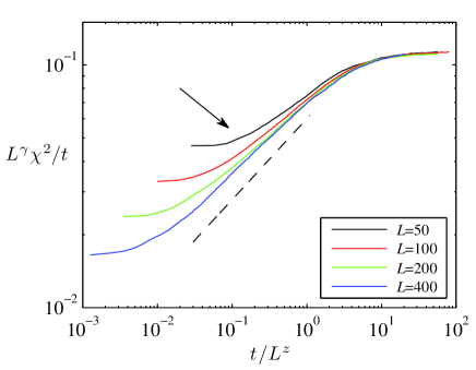
Figure 1: (Color online) Rescaled variance $\chi^{2}$ of the fluctuations of the maximum FTLE in a chain of Hénon maps (see the text for the parameter values). The various curves correspond to $L=50$, 100, 200, and 400. The exponent values used for the data collapse are $z=3/2$, $\gamma=1/2$; while the slope of the straight line is 1/3.

III.1 One-dimensional systems ($d=1$)

The first model we analyze is a chain of Hénon maps, whose LE fluctuations have been recently studied in Ref. kuptsov11 . The model writes

$$x_{n}(t+1)=a-[x_{n}(t)+\epsilon{\cal D}x_{n}(t)]^{2}+bx_{n}(t-1)$$ (17)

where ${\cal D}x_{n}\equiv x_{n-1}-2x_{n}+x_{n+1}$ is the discrete Laplacian operator, $n=1,\ldots,L$, and we select $a=1.4$, $b=0.3$, $\epsilon=0.025$. In Fig. 1 we plot $L^{\gamma}\chi^{2}/t$ , obtaining that for different system sizes the data indeed collapse for $\gamma=1/2$ onto a dynamic scaling function $\mathcal{G}$ that follows Eq. (7) and the predicted asymptotes both above ($t\gg L^{z}$) and below ($1\ll t\ll L^{z}$) the crossover time. In particular, the very good data collapse observed at long times validates Eq. (9). $\gamma=1/2$ was also observed in Ref. kuptsov11 where the Euclidean norm was used to measure vector metrics in tangent space, instead of the 0-norm considered in this paper. This confirms that the norm choice does not affect the stationary behavior. At shorter times, finite-size corrections are more sizable, but one can nevertheless appreciate an increasing quality of the data collapse with $L$. The initial slope increases with $L$ and approaches the theoretical prediction $\nu=1/3$. Notice that this means that $\chi^{2}$ initially grows as $t^{4/3}$, i.e. the Lyapunov dynamics is superdiffusive in the intermediate regime before saturation of fluctuations.

We have also studied numerically the Lorenz-96 model lorenz96

$$\frac{dy_{i}}{dt}=-y_{i}-y_{i-1}(y_{i-2}-y_{i+1})+F\,,$$ (18)

a time-continuous toy-model of the atmosphere that represents the value of a scalar variable on a mid-latitude. The data collapse shown in Fig. 2 confirms that the diffusion of the largest LE is well described by Eq. (7). The only difference with respect to the previous model is that, as the arrow indicates, the curves converge towards the asymptotic shape from below.

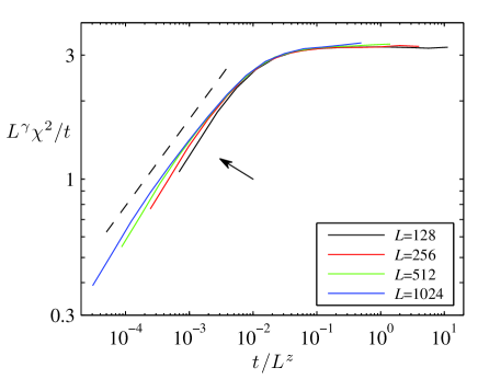
Figure 2: (Color online) Rescaled variance $\chi^{2}$ in the Lorenz-96 model, Eq. (18), with $F=8$. The slope of the straight line is $1/3$.

As a last example of a (pseudo) 1d system, we present our numerical results for a very different type of chaotic system: a model with delayed feedback. For many models of this type, the main LV scales as in typical 1d spatio-temporal chaotic systems pik98 ; pazo_lopez10 , after identifying the delay $T$ with the system size $L$. Note that one also must rescale the time axis $t$ by a factor $1/T$, as it is so for the Lyapunov spectrum farmer82 . More specifically, we have carried out simulations of the Mackey-Glass model mg77 ,

$$\frac{dy(t)}{dt}=-ay(t)+b\frac{y(t-T)}{1+y(t-T)^{10}}\,.$$ (19)

The results are plotted in Fig. 3. Apart from a relatively slow convergence they are again in agreement with our theoretical predictions.

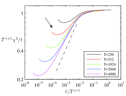
Figure 3: (Color online) Rescaled variance $\chi^{2}$ in the Mackey-Glass model, Eq. (19), with $a=0.1$ and $b=0.2$ (like in pazo_lopez10 ). The slope of the straight line is $1/3$.

III.2 Two-dimensional systems ($d=2$)

It is very instructive to check the theoretical predictions in two-dimensional models since the KPZ critical exponents depend on the spatial dimension. Current numerical capabilities allow us to study a two-dimensional lattice composed by $L^{2}$ coupled logistic maps (on a torus geometry)

$$u_{n}(t+1)=(1-\epsilon)f[u_{n}(t)]+\epsilon\sum_{m\in{\cal N}(n)}f[u_{m}(t)]$$ (20)

where $f[u(t)]\equiv 4u(t)[1-u(t)]$ and the sum is over the set ${\cal N}$ of nearest neighbors.

In two dimensions, only numerical estimates of the KPZ scaling exponents $\alpha$ and $z$ are available. The best estimations forrest90 are $\alpha\simeq 0.387$, and $z\simeq 1.613$, so that we predict $\gamma\simeq 0.839$ and $\nu\simeq 0.720$ for the wandering exponent in (9) and the time exponent in (14), respectively. Numerical results for the dynamic scaling function are plotted in Fig. 4. The data collapse is excellent, confirming again the validity of our theoretical arguments. Notice that the LE fluctuations decay with the system size faster in 2d than in 1d since $\gamma$ is larger. At short times one observes again the presence of strong finite-size corrections but one can nevertheless appreciate the predicted scaling behavior $\sim t^{0.72}$ as the system size is increased.

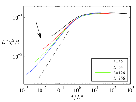
Figure 4: (Color online) Rescaled variance $\chi^{2}$ of the fluctuations of the maximum FTLE for a 2d lattice of logistic maps with $\epsilon=0.1$ (the different curves correspond to $L=32$, 64, 128, and 256 — from top to bottom. The exponent values used for the data collapse are $z=1.613$ and $\gamma=0.839$; while the slope of the straight line is 0.72.

IV The bulk of the Lyapunov spectrum: Numerical Results

In this section, we investigate numerically the scaling behavior of $D_{ii}$ for $i>1$, including the intermediate time regime before saturation, by revisiting the chain of Hénon maps and studying the Lorenz-96 model.

It is worth recalling that, in the limit of large system-sizes, the LEs depend on the integrated density $\rho=(i-0.5)/L$ (in this section we limit ourselves to studying one-dimensional systems). As a consequence, a meaningful comparison of LVs for different system sizes must be made by selecting the index $i$ which corresponds to the same density $\rho$. Since $i$ is, by definition, an integer variable in the following we interpolate between the two nearest integers that correspond to the given $\rho$-value.

IV.1 Chain of Hénon maps

In Fig. 5 we plot the results of simulations performed with the chain of Hénon maps for $\rho=0.25$. This $\rho$-value is (i) sufficiently distant from the singularity at $\rho=0$ to avoid crossover problems, and (ii) small enough to be computationally achievable in large systems foot2 . We monitor the evolution of $d\chi^{2}/dt$ rather than $\chi^{2}/t$. The two quantities would be equally valid as both obey the same scaling relation (7), but we prefer to use the former one, since it converges faster (i.e. for smaller values of $t$) to the asymptotic value. The solid curves in Fig. 5 correspond to simulations performed with the 0-norm for different system sizes. Altogether, the good data collapse confirms our scaling analysis, with $\gamma\simeq 0.865$ (close to the numerical value 0.85 measured in kuptsov11 ) and $z=1$ (as determined from direct LV studies szendro07 ; pazo08 ). Moreover, the initial growth agrees with the theoretical prediction (see the dashed line, whose slope is $\nu=(d-\gamma)/z\simeq 0.135$).

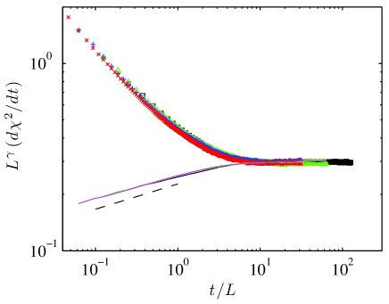
Figure 5: (Color online) Scaled FTLE fluctuations in a chain of Hénon maps (17), for $\rho=0.25$. The exponent $\gamma$ is set equal to $\gamma=0.865$. The solid curves (which correspond to $L=40$, 80, and 160) have been obtained for the 0-norm. The various symbols (squares, triangles, pluses, and crosses correspond to $L=40$, 80, 160 and 320, respectively) are obtained by using the Euclidean norm of the Gram-Schmidt LVs. The dashed line corresponds to a power law growth $(t/L^{z})^{\nu}$ with $\nu=0.135$ and $z=1$.

For comparison, in Fig. 5 we plot also the results obtained by computing the FTLE fluctuations obtained from the standard Gram-Schmidt orthogonalization procedure (see the symbols). They do not only correspond to a different way of computing the LEs, but also to a different norm (namely, the Euclidean or 2-norm). One can see that the asymptotic value of the diffusion coefficient fully agrees with the previous results: this is consistent with the expectations that long-time LEs are independent of the norm adopted and this extends to their fluctuations too. The shape of the corresponding dynamic scaling-function is, however, very different for both metrics, as expected. In fact, the LEs exhibit a sub-diffusive transient rather than super-diffusive behavior if the Euclidean metric is used.

Besides estimating the exponent $\gamma$, we have directly determined $2\alpha$ from the covariant LVs for $\rho$-values below 1, in order to test the validity of our main relation (9). The best estimation of $\alpha$ is typically obtained from the structure factor (power spectral density) of $h$, which follows a power-law decay due to its self-affine character,

$${\cal S}(k)\equiv\lim_{t\to\infty}\langle\hat{h}(k,t)\hat{h}(-k,t)\rangle\sim k^{-(2\alpha+1)}\,,$$ (21)

where $\hat{h}$ is the Fourier transform. A general representation is portrayed in Fig. 6, where the effective value of $2\alpha$ is plotted versus $\rho$ for different system sizes. In the bulk (i.e. for $0<\rho<1$), the data reveals a clear tendency to flatten towards $2\alpha\approx 0.16$ for increasing the system-size. This $\alpha$-value corresponds to $\gamma\approx 0.84$, to be compared with the direct estimate $\gamma=0.865$. This agreement, besides validating relation (9), hints at a possible universal behavior of the LV structure in the bulk of the spectrum. A careful numerical analysis (analogous to that described in Fig. 5) for $\rho=0.75$ (data not shown) further confirms that $\gamma$ is independent of $\rho$.

Appreciable deviations from the basal value $2\alpha\approx 0.16$ are clearly visible in Fig. 6 in the vicinity of the two extreme values $\rho\to 0$ and $\rho\to 1$. For $\rho\ll 1$, we know that the first LV follows KPZ scaling, $2\alpha=1$, and the data must show a cross-over towards such a different scaling, when $\rho=0.5/L\approx 0$ is approached. A similar behavior is found for $\rho=1$. Note that this value does not correspond to the smallest LE (which is obtained for $\rho=2$, as there are $2L$ exponents in a system of size $L$), but rather to the edge of the band of positive LEs. In fact, for these parameter values there exists a gap between the positive and negative bands of LEs: the singularity for $\rho=1$ thus reinforces the idea that band edges are characterized by a quantitatively different behavior, although here we do not see a direct way to map the evolution onto, e.g., KPZ dynamics.

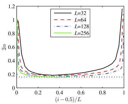
Figure 6: (Color online) Estimation of $2\alpha$ vs. $\rho$ for the LVs in a chain of Hénon maps obtained from the structure factors of the LVs by linear fitting (in log-log scale) of the 3 smallest wavenumbers. The values of $i$ used in the $x$-axis correspond to the positive LEs, save for $L=256$ in which case only the first 128 LEs have been considered due to computational limitations. The dotted line indicates $2\alpha=0.16$.

IV.2 Lorenz-96 model

The most intriguing message that arises from the study of the Hénon maps is the possibly universal scaling behavior of the bulk LVs. Given the relevance of such an observation, we have studied also the Lorenz-96 model (18). Being a continuous-time system, simulations are heavier than in the previous case and for this reason we have been able to carry out extensive simulations only for $\rho=0.1$ which is nevertheless far enough from $\rho=0$ to draw meaningful conclusions. The results for $L$ up to 256 for the 0-norm and covariant LVs, and up to 512 for the Gram-Schmidt LVs, are plotted in Fig. 7. The good data collapse confirms that the dynamic exponent is $z=1$ as in the previous model. As for $\gamma$, we find a slightly different value, namely $\gamma=0.897$ (to be compared with $\gamma=0.865$). So far it is not possible to determine whether this difference is significative or just due to strong model-dependent finite-size effects hiding a universal system-independent value. However, the closeness of both numbers suggests that $\gamma$ is universal in the bulk Lyapunov spectrum.

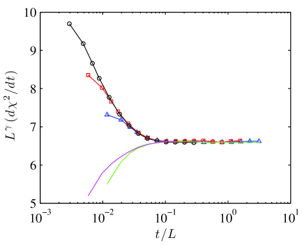
Figure 7: (Color online) Scaled FTLE fluctuations in the Lorenz-96 model (18), for $\rho=0.1$. The exponent $\gamma$ is set equal to $\gamma=0.897$. The solid curves, corresponding to $L=128$ and 256 have been obtained from the covariant LVs using the 0-norm. The various symbols (triangles, squares, and circles correspond to $L=128$, 256, and 512, respectively) are obtained by using the Euclidean norm during the forward iteration of the Gram-Schmidt LVs.

We have also determined the values of $\alpha$ from the structure factors ${\cal S}(k)$ of the LV-surfaces. The values of $2\alpha$ for the positive LEs are plotted in Fig. 8. As shown above for the chain of Hénon maps, here the curve also becomes increasingly flat as the system size grows except for the points close to $\rho=0$ and $\rho\simeq 0.33$: (i) $\rho=0$ corresponds to the first LE, where we know that $2\alpha=1$; (ii) $\rho\simeq 0.33$ corresponds to the vanishing Lyapunov exponent pazo08 , so that ${\cal S}(k)\sim k^{0}$, i.e. $2\alpha=-1$. These results suggest the existence of a common $\alpha$ for the bulk in the thermodynamic limit. Our best estimation is $2\alpha\simeq 0.13$, not far from the estimation $0.15$ in pazo08 . Moreover, assuming $z=1$, the value of $\gamma$ expected via Eq. (9) is 0.87, which is relatively close to the value $0.897$ observed in Fig. 7.

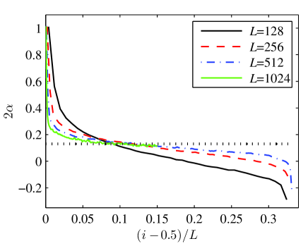
Figure 8: (Color online) Estimation of $2\alpha$ vs. $\rho$ for the Lorenz-96 model obtained from the structure factors of the LVs by linear fitting (in log-log scale) of the 3 smallest wavenumbers. The values of $i$ used in the $x$-axis correspond to the positive LEs, save for $L=1024$ in which case only the 152 largest LEs have been considered due to computational limitations. The dotted line indicates $2\alpha=0.13$.

V Conclusions and open problems

Altogether, in this paper we have shown that the analogy between roughening phenomena and LV dynamics in spatially extended systems is rather fruitful in that it allows relating the scaling behavior of the LE diffusion coefficients with the roughness exponents of the corresponding vectors. Numerical simulations of various models support the general scaling relation (7) and of its asymptotic behavior (8) and (14). With reference to the first LV, our analysis confirms the validity of the relationship with the KPZ equation in dissipative systems.

More intriguing is the question of the scaling behavior for the bulk of the Lyapunov spectrum. Our studies of Hénon maps and of the Lorenz-96 model reveal that in both cases, independently of $\rho$, $z=1$ and $\alpha\approx 0.07$. Nonetheless, small but not-so-negligible differences for the latter exponent are observed.

Two questions are, therefore, still open in the case of the fluctuations of the bulk LEs: (i) whether $\alpha$ is strictly larger than zero ($\gamma<1$) in the thermodynamic limit; (ii) the very existence of a single universality class. The $\gamma<1$ issue arises from the comparison with the cross-correlations of different LEs– namely, the scaling of the off-diagonal terms $D_{ij}$ with $i\neq j$. In Ref. kuptsov11 such terms have been found to scale as $1/L$, i.e. their $\gamma$-value is 1. This finding has been interpreted as the evidence of an extensive behavior of the large deviation function (which is proportional to the inverse of $\bf D$). On the one hand, it is strange that the diagonal terms scaling differs from that of the off-diagonal ones. On the other hand, the very fact that $\gamma<1$ implies that $\alpha>0$. This, in turn, indicates a strong localization of the covariant LV, a property that has been observed in different models by using different methods szendro07 ; ginelli07 . On the basis of the results derived in this paper for the Hénon maps (that are more reliable than those for the Lorenz-96 model) we feel confident in stating that $\gamma<1$. In order to draw firmer conclusions, however, we believe that it is necessary to make some substantial progress on the theoretical side by either identifying a minimal stochastic model of the LV dynamics for $i\gg 1$ (such as the KPZ equation for the first vector), or by resorting to new results within the field of random matrices.

- (1) E. Ott, Chaos in Dynamical Systems (Cambridge University Press, Cambridge, 1993).
- (2) D. Ruelle, Publ. Math. IHES 50, 27 (1979).
- (3) J.-P. Eckmann and D. Ruelle, Rev. Mod. Phys. 57, 617 (1985).
- (4) B. Legras and R. Vautard, in Proc. Seminar on Predictability Vol. I, ECWF Seminar, edited by T. Palmer (ECMWF, Reading, UK, 1996), pp. 135–146.
- (5) K. A. Takeuchi, F. Ginelli, and H. Chaté, Phys. Rev. Lett. 103, 154103 (2009).
- (6) H. -L. Yang et al., Phys. Rev. Lett. 102, 074102 (2009).
- (7) H. -L. Yang, G. Radons, and H. Kantz, Phys. Rev. Lett. 109, 244101 (2012).
- (8) Strictly speaking, the average over different trajectories is not needed in the infinite-time limit. We prefer, however, to keep the angular-brackets since almost everywhere in this paper, we refer to finite-time quantities.
- (9) P. V. Kuptsov and A. Politi, Phys. Rev. Lett. 107, 114101 (2011).
- (10) A. S. Pikovsky and J. Kurths, Phys. Rev. E 49, 898 (1994).
- (11) A. Pikovsky and A. Politi, Nonlinearity 11, 1049 (1998).
- (12) A. Pikovsky and A. Politi, Phys. Rev. E 63, 036207 (2001).
- (13) I. G. Szendro, D. Pazó, M. A. Rodríguez, and J. M. López, Phys. Rev. E 76, 025202(R) (2007).
- (14) D. Pazó, I. G. Szendro, J. M. López, and M. A. Rodríguez, Phys. Rev. E 78, 016209 (2008).
- (15) A.-L. Barabási and H. E. Stanley, Fractal Concepts in Surface Growth (Cambridge University Press, Cambridge, 1995).
- (16) J. M. López, M. Pradas, and A. Hernández-Machado, Phys. Rev. E 82, 031127 (2010).
- (17) J. Krug, Phys. Rev. A 44, R801 (1991).
- (18) M. Kardar, G. Parisi, and Y.-C. Zhang, Phys. Rev. Lett. 56, 889 (1986).
- (19) E. N. Lorenz, in Proc. Seminar on Predictability Vol. I, ECMWF Seminar, edited by T. Palmer (ECMWF, Reading, UK, 1996), pp. 1–18.
- (20) D. Pazó and J. M. López, Phys. Rev. E 82, 056201 (2010).
- (21) J. D. Farmer, Physica D 4, 366 (1982).
- (22) M. C. Mackey and L. Glass, Science 197, 287 (1977).
- (23) B. M. Forrest and L.-H. Tang, Phys. Rev. Lett. 64, 1405 (1990).
- (24) In fact, the number of operations needed to compute the -th LE is of the order of , where is the phase-space dimensionality — here — and the number of orthogonalizations to be performed (at variance with the computation of the surface square width , a much larger statistics is here needed to determine the LE fluctuations ).
- (25) F. Ginelli et al., Phys. Rev. Lett. 99, 130601 (2007).