Detecting Anomalous Activity on Networks with
the Graph Fourier Scan Statistic111This research is supported in part by AFOSR under grant FA9550-10-1-0382, NSF under grants DMS-1223137 and IIS-1116458.

James Sharpnack Department of Mathematics, University of California San Diego Alessandro Rinaldo Department of Statistics, Carnegie Mellon University Aarti Singh Department of Statistics, Carnegie Mellon University
Abstract

We consider the problem of deciding, based on a single noisy measurement at each vertex of a given graph, whether the underlying unknown signal is constant over the graph or there exists a cluster of vertices with anomalous activation. This problem is relevant to several applications such as surveillance, disease outbreak detection, biomedical imaging, environmental monitoring, etc. Since the activations in these problems often tend to be localized to small groups of vertices in the graphs, we model such activity by a class of signals that are supported over a (possibly disconnected) cluster with low cut size relative to its size. We analyze the corresponding generalized likelihood ratio (GLR) statistics and relate it to the problem of finding a sparsest cut in the graph. We develop a tractable relaxation of the GLR statistic based on the combinatorial Laplacian of the graph, which we call the graph Fourier scan statistic, and analyze its properties. We show how its performance as a testing procedure depends directly on the spectrum of the graph, and use this result to explicitly derive its asymptotic properties on a few significant graph topologies. Finally, we demonstrate theoretically and with simulations that the graph Fourier scan statistic can outperform naรฏve testing procedures based on global averaging and vertex-wise thresholding. We also demonstrate the usefulness of the GFSS by analyzing groundwater Arsenic concentrations from a U.S.ย Geological Survey dataset.

1 Introduction

In this article, we will take a statistical approach to detecting signals that are localized over a graph. Signal detection on graphs is relevant in a variety of scientific areas, such as surveillance, disease outbreak detection, biomedical imaging, detection using a sensor network, gene network analysis, environmental monitoring and malware detection over a computer network. Recently, the use of graphs to extend traditional methods of signal processing to irregular domains has been proposed [SNF+13, SM14, CM06, Mur07]. While this work has largely focused on extending Fourier and wavelet analysis to graphs, little is known about the statistical efficiency of the recently proposed methodology. We show that the Fourier transform over graphs, defined in [HVG11], can be used to detect anomalous patterns over graphs by constructing the Graph Fourier Scan Statistic (GFSS), a novel statistic based on spectral graph theory. We demonstrate the connection between the GFSS and the recently proposed Spectral Scan Statistic [SRS13], and provide strong theoretical guarantees.

Throughout this work, we will assume that there is a known, fixed, undirected graph with p๐‘p vertices (denoted by the set V={1,โ€ฆ,p}๐‘‰1โ€ฆ๐‘V=\{1,\ldots,p\}), m๐‘šm edges denoted by pairs (i,j)โˆˆEโŠ†Vร—V๐‘–๐‘—๐ธ๐‘‰๐‘‰(i,j)\in E\subseteq V\times V, and pร—p๐‘๐‘p\times p weighted adjacency matrix ๐–๐–\mathbf{W} (where the weight Wi,j=Wj,iโ‰ฅ0subscript๐‘Š๐‘–๐‘—subscript๐‘Š๐‘—๐‘–0W_{i,j}=W_{j,i}\geq 0 denotes the โ€˜strengthโ€™ of the connection between vertices (i,j)โˆˆE๐‘–๐‘—๐ธ(i,j)\in E). Assume that we observe a single high-dimensional measurement ๐ฒ๐ฒ\mathbf{y} over the graph, whereby for each vertex of the graph, iโˆˆV๐‘–๐‘‰i\in V, we make a single, Gaussian-distributed observation yisubscript๐‘ฆ๐‘–y_{i}. In the context of sensor networks, the measurements yisubscript๐‘ฆ๐‘–y_{i} are the values reported by each sensor, and the edge weights reflect beliefs about how similar the measurements of two sensors should be. The measurements yisubscript๐‘ฆ๐‘–y_{i} are noisy, and we are interested in determining if there is a region within the network where these observations are abnormally high. Specifically, we are concerned with the basic but fundamental task of deciding whether there is a โ€˜clusterโ€™ of vertices within the graph, CโŠ‚V๐ถ๐‘‰C\subset V, such that in expectation the observation, ๐”ผโ€‹[yi]๐”ผdelimited-[]subscript๐‘ฆ๐‘–\mathbb{E}[y_{i}], is larger for iโˆˆC๐‘–๐ถi\in C than for iโˆ‰C๐‘–๐ถi\notin C. In Section II, we will define precisely our statistical framework, including the assumptions placed on the cluster C๐ถC and observations ๐ฒ๐ฒ\mathbf{y} in relation to the graph. In order to motivate the problem and introduce the GFSS, let us consider the following real data example.

1.A Arsenic Ground-water Concentrations in Idaho

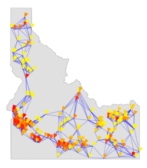
Ground-water contamination remains a serious issue globally, where aging infrastructure, shifting population densities, and climate change are among the contributing factors. A study published in 1999, reports levels of Arsenic (As) contamination measured in 20,043 wells throughout the United States [FWW+99]. In order to illustrate the usefulness of the GFSS, we analyze the As concentration with the purpose of determining if there is a region that has elevated incidence of high As levels. We will focus on the tested wells within Idaho, which was selected arbitrarily from the other US states. We construct a graph between the wells, where each vertex is a tested well, by creating an edge between two vertices (wells) if either is the k๐‘˜kth nearest neighbor of the other (See Figure 1). For easy visualization, we subsampled the wells by randomly selecting 219 (roughly 10%) of the 2,191 of the Idaho wells. We preprocessed the data by forming the indicator variable, yisubscript๐‘ฆ๐‘–y_{i}, which was 111 if the measurement made at the i๐‘–ith well was greater than 10 ppm and 00 otherwise (and we will denote the p๐‘p dimensional vector, ๐ฒ๐ฒ\mathbf{y}). We then applied a standardization which we describe in Section VI.A. The statistical problem that we address in this paper is testing if there is a well-connected set of wells, C๐ถC, such that the measurements, ๐ฒ๐ฒ\mathbf{y}, are abnormally high within the active set C๐ถC.

ย ย ย ย ย ย ย ย ย 

Refer to caption
Refer to caption
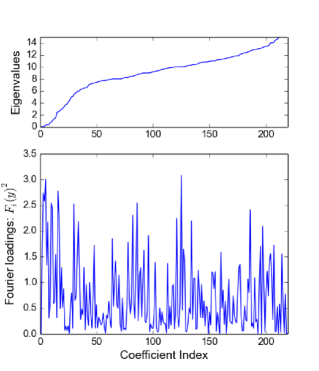
Figure 1: (Ground-water Arsenic Concentrations) The As concentrations within Idaho after (left) where red depicts higher concentrations and yellow depicts lower concentrations. The ordered eigenvalues of the well network are plotted (top right) and the Fourier loadings {โ„ฑiโ€‹(๐ฒ)2=(๐ฎiโŠคโ€‹๐ฒ)2}i=1219superscriptsubscriptsubscriptโ„ฑ๐‘–superscript๐ฒ2superscriptsuperscriptsubscript๐ฎ๐‘–top๐ฒ2๐‘–1219\{\mathcal{F}_{i}(\mathbf{y})^{2}=(\mathbf{u}_{i}^{\top}\mathbf{y})^{2}\}_{i=1}^{219} are plotted (bottom right). The index in the x-axis for the eigenvalues and Fourier loadings match so that the i๐‘–ith index corresponds to the pair ฮปi,๐ฎisubscript๐œ†๐‘–subscript๐ฎ๐‘–\lambda_{i},\mathbf{u}_{i}.

1.B Graph Fourier Scan Statistic

Traditional statistical methods, such as wavelet denoising (i.e.ย Haar and Daubechies wavelets) that employ the standard multi-resolution analysis (see [HKTP98]) are not adapted to irregular domains and sensor distributions that are not grid-like. With this in mind, a natural algorithm for the detection of such anomalous clusters of activity is the generalized likelihood ratio test (GLRT) (also known as the scan statistic or matched filter). Under a signal plus Gaussian noise model, this procedure entails scanning over all permitted clusters and hence is computationally very intensive. In [SRS13], the Spectral Scan Statistic (SSS) was proposed as a relaxation of the combinatorial GLRT. The statistical power of the detector, constructed by thresholding the SSS, was characterized using spectral graph theory. In this paper, we propose another detector which is a low-pass filter based on the graph Fourier transform. We will show that the resulting Graph Fourier Scan Statistic (GFSS), is in fact a further relaxation of the SSS, but because of its particular form it allows us to very precisely characterize its statistical power and construct an adaptive counterpart.

We will begin by introducing a graph Fourier transform, which has been previously proposed in [HVG11] (but other transforms have been proposed, as in [SM14]). Through the graph Fourier transform, we will define the GFSS, which we introduce next. Define the combinatorial Laplacian matrix ฮ”=๐ƒโˆ’๐–ฮ”๐ƒ๐–\Delta=\mathbf{D}-\mathbf{W}, where ๐ƒ=diagโ€‹{di}i=1p๐ƒdiagsuperscriptsubscriptsubscript๐‘‘๐‘–๐‘–1๐‘\mathbf{D}={\rm diag}\{d_{i}\}_{i=1}^{p} is the diagonal matrix of vertex degrees, di=โˆ‘j=1pWi,jsubscript๐‘‘๐‘–superscriptsubscript๐‘—1๐‘subscript๐‘Š๐‘–๐‘—d_{i}=\sum_{j=1}^{p}W_{i,j}. We will denote the eigenvalues and eigenvectors of ฮ”ฮ”\Delta with {ฮปi,๐ฎi}i=1psuperscriptsubscriptsubscript๐œ†๐‘–subscript๐ฎ๐‘–๐‘–1๐‘\{\lambda_{i},\mathbf{u}_{i}\}_{i=1}^{p} respectively, where we order the eigenvalues in increasing order. Hence, if ๐”๐”\mathbf{U} is the pร—p๐‘๐‘p\times p matrix where the i๐‘–ith column is the eigenvector ๐ฎisubscript๐ฎ๐‘–\mathbf{u}_{i} and ฮ›=diagโ€‹{ฮปi}i=1pฮ›diagsuperscriptsubscriptsubscript๐œ†๐‘–๐‘–1๐‘\Lambda={\rm diag}\{\lambda_{i}\}_{i=1}^{p} then we have

ฮ”=๐”โ€‹ฮ›โ€‹๐”โŠค.ฮ”๐”ฮ›superscript๐”top\Delta=\mathbf{U}\Lambda\mathbf{U}^{\top}.

For the measurement vector ๐ฒ๐ฒ\mathbf{y} over the vertices, the graph Fourier transform is โ„ฑโ€‹(๐ฒ)=๐”โŠคโ€‹๐ฒโ„ฑ๐ฒsuperscript๐”top๐ฒ\mathcal{F}(\mathbf{y})=\mathbf{U}^{\top}\mathbf{y}. Then the coordinate โ„ฑiโ€‹(๐ฒ)=๐ฎiโŠคโ€‹๐ฒsubscriptโ„ฑ๐‘–๐ฒsuperscriptsubscript๐ฎ๐‘–top๐ฒ\mathcal{F}_{i}(\mathbf{y})=\mathbf{u}_{i}^{\top}\mathbf{y} for i๐‘–i small are the low frequency components of ๐ฒ๐ฒ\mathbf{y} and for i๐‘–i large are the high frequency components. In fact, the eigenbasis of the graph Laplacian is commonly used for statistical methods over graphs and point clouds in machine learning. Much of this work has focused on dimension reduction and clustering [BN01, NJW+02, BXKS11], there has been some work on using the Laplacian for regression and testing [NSJ07, SS10]. We demonstrate with the GFSS, and its theoretical analysis, another aspect of the Laplacian eigenbasis in a statistical context.

In order to construct the GFSS, consider a low-pass filter, G๐บG, that passes the low-frequency components of ๐ฒ๐ฒ\mathbf{y} and attenuates (shrinks) the high-frequency components,

Gโ€‹(๐ฒ)=โˆ‘i=2phโ€‹(ฮปi)โ€‹(๐ฎiโŠคโ€‹๐ฒ)โ€‹๐ฎi,hโ€‹(ฮปi)=minโก{1,ฯฮปi},formulae-sequence๐บ๐ฒsuperscriptsubscript๐‘–2๐‘โ„Žsubscript๐œ†๐‘–superscriptsubscript๐ฎ๐‘–top๐ฒsubscript๐ฎ๐‘–โ„Žsubscript๐œ†๐‘–1๐œŒsubscript๐œ†๐‘–G(\mathbf{y})=\sum_{i=2}^{p}h(\lambda_{i})(\mathbf{u}_{i}^{\top}\mathbf{y})\mathbf{u}_{i},\quad h(\lambda_{i})=\min\Big{\{}1,\sqrt{\frac{\rho}{\lambda_{i}}}\Big{\}},

where ฯ>0๐œŒ0\rho>0 is a tuning parameter. Because ฮปisubscript๐œ†๐‘–\lambda_{i} is increasing in i๐‘–i the attenuation factor, hโ€‹(ฮปi)โ„Žsubscript๐œ†๐‘–h(\lambda_{i}), is 111 for i๐‘–i small enough and is non-increasing in i๐‘–i. Then we define the Graph Fourier Scan Statistic as the energy of the attenuated signal with an adjustment for the amount of the attenuation (we let โˆฅ.โˆฅ\|.\| denote the โ„“2subscriptโ„“2\ell_{2} norm),

t^^๐‘ก\displaystyle\hat{t} =โ€–Gโ€‹(๐ฒ)โ€–2โˆ’โˆ‘i=2phโ€‹(ฮปi)2absentsuperscriptnorm๐บ๐ฒ2superscriptsubscript๐‘–2๐‘โ„Žsuperscriptsubscript๐œ†๐‘–2\displaystyle=\|G(\mathbf{y})\|^{2}-\sum_{i=2}^{p}h(\lambda_{i})^{2} (1)
=โˆ‘i=1pminโก{1,ฯฮปi}โ€‹[(๐ฎiโŠคโ€‹๐ฒ)2โˆ’1].absentsuperscriptsubscript๐‘–1๐‘1๐œŒsubscript๐œ†๐‘–delimited-[]superscriptsuperscriptsubscript๐ฎ๐‘–top๐ฒ21\displaystyle=\sum_{i=1}^{p}\min\Big{\{}1,\frac{\rho}{\lambda_{i}}\Big{\}}\left[(\mathbf{u}_{i}^{\top}\mathbf{y})^{2}-1\right].

We will explain why the first eigenvector ๐ฎ1subscript๐ฎ1\mathbf{u}_{1} is ignored in Section IV (notice that the index of the sum begins at 2). We should note here that for any graph Laplacian, ฮป1=0subscript๐œ†10\lambda_{1}=0 and u1,i=pโˆ’1/2subscript๐‘ข1๐‘–superscript๐‘12u_{1,i}=p^{-1/2} for all iโˆˆV๐‘–๐‘‰i\in V. If the GFSS is abnormally large then a large amount of the signal ๐ฒ๐ฒ\mathbf{y} is in the low-frequency components. We will see in Section IV.A that this occurs when there is a well-connected cluster C๐ถC of vertices that have an abnormally large signal.

In Figure 1, we have displayed the eigenvalues in increasing order and the squared graph Fourier coefficients (where the index of the eigenvalues matches the index of the coefficients), โ„ฑiโ€‹(๐ฒ)2subscriptโ„ฑ๐‘–superscript๐ฒ2\mathcal{F}_{i}(\mathbf{y})^{2}, for the Idaho As concentrations. Because the linear filter Gโ€‹(๐ฒ)๐บ๐ฒG(\mathbf{y}) focuses the sensing energy on the low frequency components, the GFSS will be high if the Fourier loadings โ„ฑiโ€‹(๐ฒ)2subscriptโ„ฑ๐‘–superscript๐ฒ2\mathcal{F}_{i}(\mathbf{y})^{2} are large for smaller i๐‘–i.

By forming a k-nearest neighbor (kNN) graph over all 2,191 wells in Idaho with k=8๐‘˜8k=8 and applying the GFSS with ฯ=ฮป109๐œŒsubscript๐œ†109\rho=\lambda_{109} (the 109109109th smallest eigenvalue, which was selected simply because 109=โŒŠ0.05โ€‹(2191)โŒ‹1090.052191109=\lfloor 0.05(2191)\rfloor). The GFSS statistic evaluates to 697.1697.1697.1 and we can obtain a P-value <10โˆ’5absentsuperscript105<10^{-5} by a permutation test (explained in Section VI.A). This indicates that we can be confident that the probability of obtaining a high As measurement is non-constant throughout the graph.

Recall that we also subsampled the well measurements, to form a kNN graph (k=8๐‘˜8k=8) over 219 wells (as shown in Figure 1). By selecting ฯ=ฮป10๐œŒsubscript๐œ†10\rho=\lambda_{10} which is selected by the same rule as before (10=โŒŠ0.05โ€‹(219)โŒ‹100.0521910=\lfloor 0.05(219)\rfloor), the GFSS also obtains a P-value <10โˆ’5absentsuperscript105<10^{-5}. So, despite the fact that we used 10%percent1010\% of the samples in this dataset, we can still conclude with confidence that the signal is not identically distributed over the graph. With this knowledge, targeted ground-water treatment could be recommended and further statistical analysis for locating the contamination would be warranted. After we make a thorough case for the GFSS from a theoretical perspective, we will return to the As detection example in Section VI.A.

1.C Related Work

The problem of statistical hypothesis testing of graph-structured activation has received some attention recently. The GLRT for graphs, also known as the graph scan statistic, is discussed in [Pri04]. Theoretical properties of the GLRT for some specific topologies and specific signal classes have also been derived, e.g. detecting an interval in a line graph or geometric shapes such as rectangles, disks or ellipses in a lattice graph [ACDH05], path of activation in a tree or lattice [ACCHZ08], or nonparametric shapes in a lattice graph [ACCD11]. In these settings, scanning over the entire signal class or over an epsilon-net for the signal class is often feasible and has been shown to have near-optimal statistical performance. However, for general graphs and signal classes these detectors are infeasible, either because the scan involves too many patterns or due to lack of constructive ways to obtain an epsilon-net. While there has been some work on developing fast graph subset scanning methods [SN10], these greedy methods sacrifice statistical power. Also, there is work on developing Fourier basis and wavelets for graphs (c.f. [SNF+13] and references therein), which can potentially serve as an epsilon-net, however the approximation properties of such basis are not well characterized. An exception is [SKS13a] where graph wavelets were constructed using a spanning tree and statistical properties of the corresponding wavelet detector have been characterized. In [ABBDL10], the authors consider the complete graph and study detection under some combinatorial classes such as signals supported over cliques, bi-cliques, and spanning trees. They establish lower bounds on the performance of any detector, and provide upper bounds for some simple but sub-optimal detectors such as averaging all node observations and thresholding.

We build on our previous findings in [SRS13] where the Spectral Scan Statistic was proposed as a convex spectral relaxation of the GLRT and characterize its statistical performance. In another recent work [SKS13b], we have also developed a different convex relaxation of the GLRT using Lovasz extension and characterized its properties for detecting graph-structured signals. A comparison of our prior work [SKS13a, SRS13, SKS13b] appears in [SS13]. Despite the empirical success of the SSS in [SRS13], the statistical guarantees made are in some cases dominated by the guarantees obtained for the energy test statistic (to be introduces in Section III.B) which does not take the graph structure into account. The GFSS attains superior theoretical performance which always outperforms the energy statistic (except in cases in which the graph structure is misleading). Moreover, because the GFSS is formed by attenuating high frequency components via the graph Fourier transform (as in [HVG11]), this paper provides a statistical justification for the use of the combinatorial Laplacian to derive a graph Fourier analysis. Furthermore, the SSS requires perfect knowledge of the tuning parameter ฯ๐œŒ\rho, which is not known in general. To this end, we form the adaptive GFSS, which automatically selects ฯ๐œŒ\rho. In practice, the adaptive GFSS significantly outperforms the GFSS with a heuristic choice of ฯ๐œŒ\rho. The GFSS also may be preferable to more complicated procedures because it is based on a linear filter of the measurements ๐ฒ๐ฒ\mathbf{y}, which in some computational settings may be advantageous.

1.D Contributions

Our contributions are as follows. (1) We examine a new alternative hypothesis, which we call the graph-structured H1subscript๐ป1H_{1}, which generalizes the piece-wise constant graph-structured H1subscript๐ป1H_{1} proposed in [SRS13]. (2) Following the derivation of the SSS in [SRS13], we show the relationship between the GFSS, SSS, and GLRT. (3) In our main theoretical result, we show that the performance of the GFSS depends explicitly on the spectral properties of the graph. (4) Because the GFSS requires the specification of the tuning parameter, ฯ๐œŒ\rho, we develop an adaptive version of the GFSS that automatically selects ฯ๐œŒ\rho. We extend our theory to this test. (5) Using such results we are able to characterize in a very explicit form the performance of the GFSS on a few notable graph topologies and demonstrate its superiority over detectors that do not take into account the graph structure. (6) We demonstrate the usefulness of the GFSS with the partially simulated Arsenic concentration dataset.

2 Problem Setup

Detection involves the fundamental statistical question: are we observing merely noise or is there some signal amidst this noise? While the As contamination example in Section I.A involves binary measurements, for ease of presentation, we will work with Gaussian measurements with the understanding that many of the results derived may be extended easily to binary observations via subGaussian theory. We begin by outlining the basic problem of detecting a signal in Gaussian noise, then we will dive into graph-structured signals and the corresponding detection problem. First we begin with the Gaussian sequence space model, in which we make one observation at each node of the graph, yielding a vector ๐ฒโˆˆโ„p๐ฒsuperscriptโ„๐‘\mathbf{y}\in\mathbb{R}^{p} which is modeled as

๐ฒ=๐ฑ+ฯต,๐ฒ๐ฑbold-italic-ฯต\mathbf{y}=\mathbf{x}+\bm{\epsilon}, (2)

where ๐ฑโˆˆโ„p๐ฑsuperscriptโ„๐‘\mathbf{x}\in\mathbb{R}^{p} is the unknown signal and ฯตโˆผNโ€‹(0,ฯƒ2โ€‹๐ˆp)similar-tobold-italic-ฯต๐‘0superscript๐œŽ2subscript๐ˆ๐‘\bm{\epsilon}\sim N(0,\sigma^{2}\mathbf{I}_{p}) is Gaussian noise, with ฯƒ2superscript๐œŽ2\sigma^{2} known. While the basic detection problem is to determine whether the signal ๐ฑ๐ฑ\mathbf{x} is constant or not, we analyze three different alternative hypotheses: unstructured signal, piece-wise constant graph-structured signal, and the more general graph-structured signal with differential activation.

Unstructured H1subscript๐ป1H_{1}. In order to make clear the improvements that the graph-structure affords us, we will consider the testing problem without any such structure. Throughout this paper we will also let ๐Ÿ=(1,โ€ฆ,1)11โ€ฆ1{\bf 1}=(1,\ldots,1) denote the all 111s vector, and ๐ฑยฏ=nโˆ’1โ€‹(โˆ‘i=1pxi)โ€‹๐Ÿยฏ๐ฑsuperscript๐‘›1superscriptsubscript๐‘–1๐‘subscript๐‘ฅ๐‘–1\bar{\mathbf{x}}=n^{-1}(\sum_{i=1}^{p}x_{i}){\bf 1}. We define the class of unstructured signals, parametrized by a signal strength parameter ฮผ>0๐œ‡0\mu>0, as ๐’ณUโ€‹(ฮผ)={๐ฑโˆˆโ„p:โ€–๐ฑโˆ’๐ฑยฏโ€–โ‰ฅฮผ}subscript๐’ณ๐‘ˆ๐œ‡conditional-set๐ฑsuperscriptโ„๐‘norm๐ฑยฏ๐ฑ๐œ‡\mathcal{X}_{U}(\mu)=\{\mathbf{x}\in\mathbb{R}^{p}:\|\mathbf{x}-\bar{\mathbf{x}}\|\geq\mu\}, the complement of the open ball of radius ฮผ๐œ‡\mu in the subspace orthogonal to ๐Ÿ1{\bf 1}. We consider only the subspace orthogonal to ๐Ÿ1{\bf 1} because the null is invariant under changes of ๐ฑ๐ฑ\mathbf{x} within this space. Then the basic โ€˜unstructuredโ€™ hypothesis testing problem is,

H0:๐ฑ=๐ฑยฏโ€‹ย v.s.ย โ€‹H1U:๐ฑโˆˆ๐’ณUโ€‹(ฮผ):subscript๐ป0๐ฑยฏ๐ฑย v.s.ย superscriptsubscript๐ป1๐‘ˆ:๐ฑsubscript๐’ณ๐‘ˆ๐œ‡H_{0}:\mathbf{x}=\bar{\mathbf{x}}\textrm{\quad v.s. \quad}H_{1}^{U}:\mathbf{x}\in\mathcal{X}_{U}(\mu)

Because there is no a priori structure, in this setting we are compelled to use tests that are invariant under arbitrary permutation of the coordinates of ๐ฒ๐ฒ\mathbf{y} and ๐ฑ๐ฑ\mathbf{x}. We will now outline the graph-structured alternative hypotheses.

Piece-wise constant graph-structured H1subscript๐ป1H_{1}. Following [SRS13], will assume that there are two regions of constant signal for ๐ฑ๐ฑ\mathbf{x}, namely that there exists a (possibly disconnected) subset CโŠ‚V๐ถ๐‘‰C\subset V (Cโˆ‰{โˆ…,V}๐ถ๐‘‰C\notin\{\emptyset,V\}) such that ๐ฑ๐ฑ\mathbf{x} is constant within both C๐ถC and its complement Cยฏ=V\Cยฏ๐ถ\๐‘‰๐ถ\bar{C}=V\backslash C. We consider the class of signals that are piece-wise constant on C๐ถC and Cยฏยฏ๐ถ\bar{C}, and parametrized by a signal strength parameter ฮผ๐œ‡\mu, defined as

๐’ณPโ€‹Cโ€‹(ฮผ,C)={๐ฑ=ฮฑโ€‹๐Ÿ+ฮดโ€‹๐ŸC:ฮฑ,ฮดโˆˆโ„}โˆฉ๐’ณUโ€‹(ฮผ)subscript๐’ณ๐‘ƒ๐ถ๐œ‡๐ถconditional-set๐ฑ๐›ผ1๐›ฟsubscript1๐ถ๐›ผ๐›ฟโ„subscript๐’ณ๐‘ˆ๐œ‡\mathcal{X}_{PC}(\mu,C)=\{\mathbf{x}=\alpha{\bf 1}+\delta{\bf 1}_{C}:\alpha,\delta\in\mathbb{R}\}\cap\mathcal{X}_{U}(\mu)

where ๐ŸCโˆˆโ„psubscript1๐ถsuperscriptโ„๐‘{\bf 1}_{C}\in\mathbb{R}^{p} such that ๐ŸC,i=1subscript1๐ถ๐‘–1{\bf 1}_{C,i}=1 if iโˆˆC๐‘–๐ถi\in C and 00 otherwise. The parameter ฮฑ๐›ผ\alpha can be thought of as the magnitude of the background signal and is a nuisance parameter, while ฮด๐›ฟ\delta quantifies the gap in signal between the two clusters. For the signal ๐ฑ=ฮฑโ€‹๐Ÿ+ฮดโ€‹๐ŸC๐ฑ๐›ผ1๐›ฟsubscript1๐ถ\mathbf{x}=\alpha{\bf 1}+\delta{\bf 1}_{C} to be contained in ๐’ณUโ€‹(ฮผ)subscript๐’ณ๐‘ˆ๐œ‡\mathcal{X}_{U}(\mu), it is required that โ€–๐ฑโˆ’๐ฑยฏโ€–=|C|โ€‹|Cยฏ|pโ€‹|ฮด|โ‰ฅฮผnorm๐ฑยฏ๐ฑ๐ถยฏ๐ถ๐‘๐›ฟ๐œ‡\|\mathbf{x}-\bar{\mathbf{x}}\|=\sqrt{\frac{|C||\bar{C}|}{p}}|\delta|\geq\mu.

We will not assume any knowledge of the true cluster C๐ถC, other than that it belongs to a given class ๐’žโŠ‚2V๐’žsuperscript2๐‘‰\mathcal{C}\subset 2^{V} that we define next. This class provides a good model for activations that are localized on the graph as we will see. Formally, we define, for some ฯ>0๐œŒ0\rho>0 (which is the same ฯ๐œŒ\rho in the definition of the GFSS),

๐’ž=๐’žโ€‹(ฯ)={CโŠ‚V,Cโ‰ โˆ…:๐–โ€‹(โˆ‚C)|C|โ€‹|Cยฏ|โ‰คฯp},๐’ž๐’ž๐œŒconditional-setformulae-sequence๐ถ๐‘‰๐ถ๐–๐ถ๐ถยฏ๐ถ๐œŒ๐‘\mathcal{C}=\mathcal{C}(\rho)=\left\{C\subset V,C\neq\emptyset\colon\frac{\mathbf{W}(\partial C)}{|C||\bar{C}|}\leq\frac{\rho}{p}\right\}, (3)

where โˆ‚C={(i,j)โˆˆE:iโˆˆC,jโˆˆCยฏ}๐ถconditional-set๐‘–๐‘—๐ธformulae-sequence๐‘–๐ถ๐‘—ยฏ๐ถ\partial C=\{(i,j)\in E:i\in C,j\in\bar{C}\} is the boundary of C๐ถC and ๐–โ€‹(โˆ‚C)=โˆ‘(i,j)โˆˆโˆ‚CWi,j๐–๐ถsubscript๐‘–๐‘—๐ถsubscript๐‘Š๐‘–๐‘—\mathbf{W}(\partial C)=\sum_{(i,j)\in\partial C}W_{i,j}. Note that ๐’ž๐’ž\mathcal{C} is a symmetric class in the sense that Cโˆˆ๐’ž๐ถ๐’žC\in\mathcal{C} if and only if Cยฏโˆˆ๐’žยฏ๐ถ๐’ž\bar{C}\in\mathcal{C}. The quantity pโ€‹๐–โ€‹(โˆ‚C)|C|โ€‹|Cยฏ|๐‘๐–๐ถ๐ถยฏ๐ถ\frac{p\mathbf{W}(\partial C)}{|C||\bar{C}|} is known in the graph theory literature as the cut sparsity [Vaz01] and is equivalent, up to factor of 222, to the cut expansion (๐–โ€‹(โˆ‚C)minโก{|C|,|Cยฏ|}๐–๐ถ๐ถยฏ๐ถ\frac{\mathbf{W}(\partial C)}{\min\{|C|,|\bar{C}|\}}):

๐–โ€‹(โˆ‚C)minโก{|C|,|Cยฏ|}โ‰คpโ€‹๐–โ€‹(โˆ‚C)|C|โ€‹|Cยฏ|โ‰ค2โ€‹๐–โ€‹(โˆ‚C)minโก{|C|,|Cยฏ|}๐–๐ถ๐ถยฏ๐ถ๐‘๐–๐ถ๐ถยฏ๐ถ2๐–๐ถ๐ถยฏ๐ถ\frac{\mathbf{W}(\partial C)}{\min\{|C|,|\bar{C}|\}}\leq\frac{p\mathbf{W}(\partial C)}{|C||\bar{C}|}\leq 2\frac{\mathbf{W}(\partial C)}{\min\{|C|,|\bar{C}|\}}

The cut expansion of a vertex set C๐ถC is a measure of the size of the boundary relative to the size of C๐ถC. Notice that for the same size of activation, a signal that is localized to a group of well connected nodes on the graph has a smaller cut sparsity and cut expansion than a signal which is distributed over isolated nodes. Thus, the class provides a good model for signals that are localized over the graph. Note that this definition is much less restrictive than existing work, e.g. [ACDH05] considers intervals, rectangles, ellipses, and similar geometrical shapes, or [ABBDL10] considers cliques, stars, spanning trees. The only other work which considers general non-parametric shapes is [ACCD11], however it only considers lattice graphs and it is not clear how to extend the signal class definition used in that work to general graphs.

Define the class of all piece-wise constant signals with signal strength ฮผ๐œ‡\mu and cut sparsity bounded by ฯ๐œŒ\rho as ๐’ณPโ€‹Cโ€‹(ฮผ,ฯ)=โˆชCโˆˆ๐’žโ€‹(ฯ)๐’ณPโ€‹Cโ€‹(ฮผ,C)subscript๐’ณ๐‘ƒ๐ถ๐œ‡๐œŒsubscript๐ถ๐’ž๐œŒsubscript๐’ณ๐‘ƒ๐ถ๐œ‡๐ถ\mathcal{X}_{PC}(\mu,\rho)=\cup_{C\in\mathcal{C}(\rho)}\mathcal{X}_{PC}(\mu,C). Then we will consider the hypothesis testing problem,

H0:๐ฑ=๐ฑยฏโ€‹ย v.s.ย โ€‹H1Pโ€‹C:๐ฑโˆˆ๐’ณPโ€‹Cโ€‹(ฮผ,ฯ).:subscript๐ป0๐ฑยฏ๐ฑย v.s.ย superscriptsubscript๐ป1๐‘ƒ๐ถ:๐ฑsubscript๐’ณ๐‘ƒ๐ถ๐œ‡๐œŒH_{0}:\mathbf{x}=\bar{\mathbf{x}}\textrm{\quad v.s. \quad}H_{1}^{PC}:\mathbf{x}\in\mathcal{X}_{PC}(\mu,\rho).

Because the piece-wise constant assumption may be restrictive, we will endeavor to generalize it to a larger alternative space.

Graph-structured H1subscript๐ป1H_{1}. We now consider a more general form of alternative, in which the signal is graph-structured, but not necessarily constant over clusters of activation. Specifically, we will assume that there is again a true cluster Cโˆˆ๐’žโ€‹(ฯ)๐ถ๐’ž๐œŒC\in\mathcal{C}(\rho) within which the signal differs little and across which the signal differs highly. Formally, we define the class of graph-structured signals as

๐’ณSโ€‹(ฮผ,ฯ)={๐ฑโˆˆโ„p:|๐ŸCโŠคโ€‹๐ฑ|C|โˆ’๐ŸCยฏโŠคโ€‹๐ฑ|Cยฏ||โ€‹|C|โ€‹|Cยฏ|pโ‰ฅฮผ,Cโˆˆ๐’ž}.subscript๐’ณ๐‘†๐œ‡๐œŒconditional-set๐ฑsuperscriptโ„๐‘formulae-sequencesuperscriptsubscript1๐ถtop๐ฑ๐ถsuperscriptsubscript1ยฏ๐ถtop๐ฑยฏ๐ถ๐ถยฏ๐ถ๐‘๐œ‡๐ถ๐’ž\mathcal{X}_{S}(\mu,\rho)=\left\{\mathbf{x}\in\mathbb{R}^{p}:\left|\frac{{\bf 1}_{C}^{\top}\mathbf{x}}{|C|}-\frac{{\bf 1}_{\bar{C}}^{\top}\mathbf{x}}{|\bar{C}|}\right|\sqrt{\frac{|C||\bar{C}|}{p}}\geq\mu,C\in\mathcal{C}\right\}.

Notice that if ๐ฑโˆˆ๐’ณSโ€‹(ฮผ,ฯ)๐ฑsubscript๐’ณ๐‘†๐œ‡๐œŒ\mathbf{x}\in\mathcal{X}_{S}(\mu,\rho) then โ€–๐ฑโˆ’๐ฑยฏโ€–โ‰ฅฮผnorm๐ฑยฏ๐ฑ๐œ‡\|\mathbf{x}-\bar{\mathbf{x}}\|\geq\mu, so ๐’ณSโ€‹(ฮผ,ฯ)โŠ‚๐’ณUโ€‹(ฮผ)subscript๐’ณ๐‘†๐œ‡๐œŒsubscript๐’ณ๐‘ˆ๐œ‡\mathcal{X}_{S}(\mu,\rho)\subset\mathcal{X}_{U}(\mu). Furthermore, if ๐ฑ=ฮฑโ€‹๐Ÿ+ฮดโ€‹๐ŸCโˆˆ๐’ณPโ€‹Cโ€‹(ฮผ,ฯ)๐ฑ๐›ผ1๐›ฟsubscript1๐ถsubscript๐’ณ๐‘ƒ๐ถ๐œ‡๐œŒ\mathbf{x}=\alpha{\bf 1}+\delta{\bf 1}_{C}\in\mathcal{X}_{PC}(\mu,\rho) then

|๐ŸCโŠคโ€‹๐ฑ|C|โˆ’๐ŸCยฏโŠคโ€‹๐ฑ|Cยฏ||=|ฮด|.superscriptsubscript1๐ถtop๐ฑ๐ถsuperscriptsubscript1ยฏ๐ถtop๐ฑยฏ๐ถ๐›ฟ\left|\frac{{\bf 1}_{C}^{\top}\mathbf{x}}{|C|}-\frac{{\bf 1}_{\bar{C}}^{\top}\mathbf{x}}{|\bar{C}|}\right|=|\delta|.

Hence, ๐’ณPโ€‹Cโ€‹(ฮผ,ฯ)โŠ‚๐’ณSโ€‹(ฮผ,ฯ)subscript๐’ณ๐‘ƒ๐ถ๐œ‡๐œŒsubscript๐’ณ๐‘†๐œ‡๐œŒ\mathcal{X}_{PC}(\mu,\rho)\subset\mathcal{X}_{S}(\mu,\rho). This induces the following hypothesis testing problem,

H0:๐ฑ=๐ฑยฏโ€‹ย v.s.ย โ€‹H1S:๐ฑโˆˆ๐’ณSโ€‹(ฮผ,ฯ).:subscript๐ป0๐ฑยฏ๐ฑย v.s.ย superscriptsubscript๐ป1๐‘†:๐ฑsubscript๐’ณ๐‘†๐œ‡๐œŒH_{0}:\mathbf{x}=\bar{\mathbf{x}}\textrm{\quad v.s. \quad}H_{1}^{S}:\mathbf{x}\in\mathcal{X}_{S}(\mu,\rho).

Whenever possible we will make statements about this non-constant alternative, for the sake of generality. We outline in Section VI.E how signals in this class may arise by subsampling vertices of the cluster C๐ถC.

2.A Distinguishability of H0subscript๐ป0H_{0} and H1subscript๐ป1H_{1}

We will analyze asymptotic conditions under which the hypothesis testing problems described above are statistically feasible, in a sense made precise in the next definition. We will assume that the size of the graph p๐‘p increases and the relevant parameters of the model, ฮผ๐œ‡\mu, ฯƒ๐œŽ\sigma, ฯ๐œŒ\rho, and eigen-spectrum of ฮ”ฮ”\Delta, change with p๐‘p as well, even though we will not make such dependence explicit in our notation for ease of readability. Our results establish conditions for asymptotic disinguishability as a function of the SNR ฮผ/ฯƒ๐œ‡๐œŽ\mu/\sigma, ฯ๐œŒ\rho, and the spectrum of the graph.

Definition 1.

For a given statistic sโ€‹(๐ฒ)๐‘ ๐ฒs({\bf y}) and threshold ฯ„โˆˆโ„๐œโ„\tau\in\mathbb{R}, let T=Tโ€‹(๐ฒ)๐‘‡๐‘‡๐ฒT=T({\bf y}) be 111 if sโ€‹(๐ฒ)>ฯ„๐‘ ๐ฒ๐œs({\bf y})>\tau and 00 otherwise. Recall that H0subscript๐ป0H_{0} and H1subscript๐ป1H_{1} index sets of probability measures by which ๐ฒ๐ฒ\mathbf{y} may be distributed. We say that the hypotheses H0subscript๐ป0H_{0} and H1subscript๐ป1H_{1} are asymptotically distinguished by the test T๐‘‡T if

supโ„™0โˆˆH0โ„™0โ€‹{T=1}โ†’0ย andย supโ„™1โˆˆH1โ„™1โ€‹{T=0}โ†’0,formulae-sequenceโ†’subscriptsupremumsubscriptโ„™0subscript๐ป0subscriptโ„™0๐‘‡10ย andย โ†’subscriptsupremumsubscriptโ„™1subscript๐ป1subscriptโ„™1๐‘‡00\sup_{\mathbb{P}_{0}\in H_{0}}\mathbb{P}_{0}\{T=1\}\rightarrow 0\quad\textrm{ and }\quad\sup_{\mathbb{P}_{1}\in H_{1}}\mathbb{P}_{1}\{T=0\}\rightarrow 0, (4)

where the limit is taken as pโ†’โˆžโ†’๐‘p\rightarrow\infty. We say that H0subscript๐ป0H_{0} and H1subscript๐ป1H_{1} are asymptotically indistinguishable if there does not exist any test for which the above limits hold. Furthermore, we say that a sequence {rp}p=1โˆžsuperscriptsubscriptsubscript๐‘Ÿ๐‘๐‘1\{r_{p}\}_{p=1}^{\infty} is a critical SNR, if for ฮผ/ฯƒ=oโ€‹(rp)๐œ‡๐œŽ๐‘œsubscript๐‘Ÿ๐‘\mu/\sigma=o(r_{p}), H0subscript๐ป0H_{0} and H1subscript๐ป1H_{1} are asymptotically indistinguishable and for ฮผ/ฯƒ=ฯ‰โ€‹(rp)๐œ‡๐œŽ๐œ”subscript๐‘Ÿ๐‘\mu/\sigma=\omega(r_{p}), H0subscript๐ป0H_{0} and H1subscript๐ป1H_{1} are asymptotically distinguishable. (We denote this with ฮผ/ฯƒโ‰rpasymptotically-equals๐œ‡๐œŽsubscript๐‘Ÿ๐‘\mu/\sigma\asymp r_{p}.)

In Section III.A we will produce a lower bound on the critical SNR, and in Section IV we will derive conditions under which the GFSS asymptotically distinguishes H0subscript๐ป0H_{0} from H1Pโ€‹Csuperscriptsubscript๐ป1๐‘ƒ๐ถH_{1}^{PC} and H1Ssuperscriptsubscript๐ป1๐‘†H_{1}^{S}. We will say that a test is adaptive if it can be performed without knowledge of ฯ๐œŒ\rho. Naturally, requiring adaptivity may inhibit the quality of our test, as it has in the detection within Sobolov-type ellipsoids [Spo96, JN12]. We will modify the GFSS to make it adaptive and prove theory regarding its performance.

3 A Lower Bound and Classical Results

Our ultimate goal is to give a theory of activity detection on general graphs. This means that our theorems should apply to all graph structures with only minor, simplifying assumptions, such as connectedness. But as a validation of the theory and methods that we propose, we will pay particular attention to the implications of our results on specific graph structures. We begin by introducing the torus graph structure that will serve as a running example for illustrations. The reader should in no way interpret this to mean that our results necessarily depend on the idiosyncrasies of the torus graph, such as edge transitivity.

Example 1.

(Torus Graph) A torus graph is a lattice or two-dimensional grid that is wrapped around so that rightmost vertices are same as leftmost vertices, and topmost vertices are same as bottom vertices. Formally, the โ„“ร—โ„“โ„“โ„“\ell\times\ell torus graph (p=โ„“2๐‘superscriptโ„“2p=\ell^{2}) is defined as follows. Let the vertex set V=(โ„คmodโ„“)2๐‘‰superscriptmoduloโ„คโ„“2V=(\mathbb{Z}\mod\ell)^{2} where points (i1,i2),(j1,j2)subscript๐‘–1subscript๐‘–2subscript๐‘—1subscript๐‘—2(i_{1},i_{2}),(j_{1},j_{2}) are connected by an edge if and only if |(i1โˆ’j1)modโ„“|+|(i2โˆ’j2)modโ„“|=1modulosubscript๐‘–1subscript๐‘—1โ„“modulosubscript๐‘–2subscript๐‘—2โ„“1|(i_{1}-j_{1})\mod\ell|+|(i_{2}-j_{2})\mod\ell|=1 (here |imodโ„“|modulo๐‘–โ„“|i\mod\ell| means the smallest absolute value of representatives). The class of clusters in the torus under consideration ๐’žโ€‹(ฯ)๐’ž๐œŒ\mathcal{C}(\rho) are those that have sparsity pโ€‹๐–โ€‹(โˆ‚C)/(|C|โ€‹|Cยฏ|)โ‰คฯ๐‘๐–๐ถ๐ถยฏ๐ถ๐œŒp\mathbf{W}(\partial C)/(|C||\bar{C}|)\leq\rho. For example, rectangles of size kร—k๐‘˜๐‘˜k\times k within the torus have cut sparsity 4โ€‹kโ€‹p/(k2โ€‹(pโˆ’k2))โ‰4/kasymptotically-equals4๐‘˜๐‘superscript๐‘˜2๐‘superscript๐‘˜24๐‘˜4kp/(k^{2}(p-k^{2}))\asymp 4/k. This means that if we would like to include rectangles of size roughly kร—k๐‘˜๐‘˜k\times k, it is sufficient that ฯโ‰4/kasymptotically-equals๐œŒ4๐‘˜\rho\asymp 4/k.

In order to understand the fundamental limitations of the activity detection problem, we review lower bounds on the performance of any testing procedure. After this information theoretic result, we will review classical theory about the detection of non-zero means under no graph constraints.

3.A Lower Bound

The following lower bound on the critical SNR was derived in [SRS13]. The first part is a simple bound on the performance of the oracle (who has knowledge of the active cluster, C๐ถC) based on the Neyman-Pearson lemma. The second part is more sophisticated and requires that the graph has symmetries that we can exploit, but it will not be satisfied by many graphs. We will later show that these conditions are satisfied by the specific graph structures that we will analyze in Section VI.

Theorem 2.

[SRS13] (a) H0subscript๐ป0H_{0} and H1Pโ€‹C,H1Ssuperscriptsubscript๐ป1๐‘ƒ๐ถsuperscriptsubscript๐ป1๐‘†H_{1}^{PC},H_{1}^{S} are asymptotically indistinguishable if ฮผ/ฯƒ=oโ€‹(1)๐œ‡๐œŽ๐‘œ1\mu/\sigma=o(1).
(b) Suppose that there is a subset of clusters ๐’žโ€ฒโŠ†2Vsuperscript๐’žโ€ฒsuperscript2๐‘‰\mathcal{C}^{\prime}\subseteq 2^{V} such that all the elements of ๐’žโ€ฒsuperscript๐’žโ€ฒ\mathcal{C}^{\prime} are disjoint, of the same size (|C|=c๐ถ๐‘|C|=c for all Cโˆˆ๐’žโ€ฒ๐ถsuperscript๐’žโ€ฒC\in\mathcal{C}^{\prime}), and

โˆ€Cโˆˆ๐’žโ€ฒ,pโ€‹๐–โ€‹(โˆ‚C)|C|โ€‹|Cยฏ|โ‰คฯ2formulae-sequencefor-all๐ถsuperscript๐’žโ€ฒ๐‘๐–๐ถ๐ถยฏ๐ถ๐œŒ2\forall C\in\mathcal{C}^{\prime},\quad\frac{p\mathbf{W}(\partial C)}{|C||\bar{C}|}\leq\frac{\rho}{2}

i.e., elements of ๐’žโ€ฒsuperscript๐’žโ€ฒ\mathcal{C}^{\prime} belong to the alternative hypothesis with ฯ/2๐œŒ2\rho/2 cut sparsity. Furthermore assume that cโ€‹|๐’žโ€ฒ|pโ†’1โ†’๐‘superscript๐’žโ€ฒ๐‘1\frac{c|\mathcal{C}^{\prime}|}{p}\rightarrow 1. H0subscript๐ป0H_{0} and H1Pโ€‹C,H1Ssuperscriptsubscript๐ป1๐‘ƒ๐ถsuperscriptsubscript๐ป1๐‘†H_{1}^{PC},H_{1}^{S} are asymptotically indistinguishable if

ฮผฯƒ=oโ€‹(|๐’žโ€ฒ|1/4)๐œ‡๐œŽ๐‘œsuperscriptsuperscript๐’žโ€ฒ14\frac{\mu}{\sigma}=o(|\mathcal{C}^{\prime}|^{1/4})

We illustrate the usefulness of the lower bound with the following example.

Example 2.

(Lower Bound for Torus) We will construct ๐’žโ€ฒsuperscript๐’žโ€ฒ\mathcal{C}^{\prime} in Theorem 2 (b) from disjoint squares of size a constant multiple of p1โˆ’ฮฒsuperscript๐‘1๐›ฝp^{1-\beta}, making |๐’žโ€ฒ|โ‰pฮฒasymptotically-equalssuperscript๐’žโ€ฒsuperscript๐‘๐›ฝ|\mathcal{C}^{\prime}|\asymp p^{\beta}. Thus, the critical SNR for H0subscript๐ป0H_{0} versus any of H1Pโ€‹C,H1Ssuperscriptsubscript๐ป1๐‘ƒ๐ถsuperscriptsubscript๐ป1๐‘†H_{1}^{PC},H_{1}^{S} for any estimator is greater than pฮฒ/4superscript๐‘๐›ฝ4p^{\beta/4}.

In [ACCD11], the authors also derive a lower bound which scales as logโก(p/|C|)๐‘๐ถ\sqrt{\log(p/|C|)} for detection of patterns on the lattice graph which include squares of size |C|๐ถ|C|. However, their results only hold for clusters consisting of a single connected component, whereas H1Pโ€‹Csuperscriptsubscript๐ป1๐‘ƒ๐ถH_{1}^{PC} allows for multiple connected components. Thus, our results indicate that detecting clusters with multiple connected components is harder than detecting a cluster with a single connected component, unless the connected component is really large i.e. the activation size |C|๐ถ|C| is of the same order as the graph size p๐‘p. In the latter case, both the bound of [ACCD11] and our result imply an SNR of oโ€‹(1)๐‘œ1o(1) is insufficient for detection on the torus graph.

The scaling with the 1/4141/4th power in our results is not a coincidence. We will see that the classical results for the unconstrained alternative hypotheses also provide a critical SNR of this form.

3.B Classical Results

In order to understand the inherent difficulty of distinguishing H0subscript๐ป0H_{0} from the unstructured alternative, H1Usuperscriptsubscript๐ป1๐‘ˆH_{1}^{U}, we will recount a result from [IS03].

Theorem 3.

The critical SNR for any test distinguishing H0subscript๐ป0H_{0} from H1Usuperscriptsubscript๐ป1๐‘ˆH_{1}^{U} is given by,

ฮผฯƒโ‰p1/4asymptotically-equals๐œ‡๐œŽsuperscript๐‘14\frac{\mu}{\sigma}\asymp p^{1/4}

and it is achieved by the energy test statistic โ€–๐ฒโˆ’๐ฒยฏโ€–22superscriptsubscriptnorm๐ฒยฏ๐ฒ22\|\mathbf{y}-\bar{\mathbf{y}}\|_{2}^{2}, when it is thresholded at quantiles of the ฯ‡pโˆ’12subscriptsuperscript๐œ’2๐‘1\chi^{2}_{p-1} distribution.

This result highlights the aforementioned 1/4141/4th power scaling in critical SNRs. One would hope that in the graph-structured setting, we can tolerate an SNR smaller than this. We will see that this is achieved by the GFSS, and by its adaptive version in most cases. For completeness, we will also look at two other test statistics. Let the statistics maxiโˆˆ[p]โก|yiโˆ’yยฏ|subscript๐‘–delimited-[]๐‘subscript๐‘ฆ๐‘–ยฏ๐‘ฆ\max_{i\in[p]}|y_{i}-\bar{y}| and ๐ŸโŠคโ€‹๐ฒsuperscript1top๐ฒ{\bf 1}^{\top}\mathbf{y} be called the max statistic and the aggregate statistic respectively. Then they have the following required SNRโ€™s for the piece-wise constant alternative structure, H1Pโ€‹Csuperscriptsubscript๐ป1๐‘ƒ๐ถH_{1}^{PC}.

Theorem 4.

(a) Consider a sequence of draws from H1C:๐ฒ=๐ฑ+ฯต:superscriptsubscript๐ป1๐ถ๐ฒ๐ฑitalic-ฯตH_{1}^{C}:\mathbf{y}=\mathbf{x}+\epsilon with ๐ฑโˆˆ๐’ณPโ€‹Cโ€‹(ฮผ,C)๐ฑsubscript๐’ณ๐‘ƒ๐ถ๐œ‡๐ถ\mathbf{x}\in\mathcal{X}_{PC}(\mu,C), for the active cluster C๐ถC. The critical SNR for H0subscript๐ป0H_{0} versus H1Csuperscriptsubscript๐ป1๐ถH_{1}^{C} of the max statistic is between the following

ฮผฯƒ=ฯ‰โ€‹(|C|),ฮผฯƒ=oโ€‹(|C|โ€‹logโกp)formulae-sequence๐œ‡๐œŽ๐œ”๐ถ๐œ‡๐œŽ๐‘œ๐ถ๐‘\frac{\mu}{\sigma}=\omega(\sqrt{|C|}),\quad\frac{\mu}{\sigma}=o(\sqrt{|C|\log p})

while the upper bound is an equality (โ‰asymptotically-equals\asymp) if logโก|C|=oโ€‹(logโกp)๐ถ๐‘œ๐‘\log|C|=o(\log p).
(b) Suppose further that the alternative H1Csuperscriptsubscript๐ป1๐ถH_{1}^{C} has the more specific form:

๐ฑC=p|C|โ€‹|Cยฏ|โ€‹ฮผโ€‹๐ŸCsubscript๐ฑ๐ถ๐‘๐ถยฏ๐ถ๐œ‡subscript1๐ถ\mathbf{x}_{C}=\sqrt{\frac{p}{|C||\bar{C}|}}\mu{\bf 1}_{C}

The critical SNR for ๐ฑ=๐ŸŽ๐ฑ0\mathbf{x}={\bf 0} versus ๐ฑ=๐ฑC๐ฑsubscript๐ฑ๐ถ\mathbf{x}=\mathbf{x}_{C} of the aggregate test statistic is ฮผ/ฯƒโ‰|Cยฏ|/|C|asymptotically-equals๐œ‡๐œŽยฏ๐ถ๐ถ\mu/\sigma\asymp\sqrt{|\bar{C}|/|C|}.

Proof.

(a) follows directly from [IS03] (Corollary 3.10). (b) This follows from the fact that under H0subscript๐ป0H_{0}, the test statistic is ๐’ฉโ€‹(0,pโ€‹ฯƒ2)๐’ฉ0๐‘superscript๐œŽ2\mathcal{N}(0,p\sigma^{2}), while under H1:๐ฑ=๐ฑC:subscript๐ป1๐ฑsubscript๐ฑ๐ถH_{1}:\mathbf{x}=\mathbf{x}_{C} it has mean (pโ€‹|C|)/|Cยฏ|โ€‹ฮผ๐‘๐ถยฏ๐ถ๐œ‡\sqrt{(p|C|)/|\bar{C}|}\mu. โˆŽ

Remark 5.

Notice that the critical SNR of the max statistic, Theorem 4 (a), can be significantly worse than the energy and aggregate statistics if |C|โ‰ฅp๐ถ๐‘|C|\geq\sqrt{p}. Otherwise the max statistic is superior. Similarly, (b) provides worse performance than the energy and max statistic if |C|โ‰คp๐ถ๐‘|C|\leq\sqrt{p}. These only hold for the piecewise constant graph structure of H1Pโ€‹Csuperscriptsubscript๐ป1๐‘ƒ๐ถH_{1}^{PC}. We state the results with the dependence on |C|๐ถ|C|, as opposed to their worst case in the class ๐’žโ€‹(ฯ)๐’ž๐œŒ\mathcal{C}(\rho), because one could apply an omnibus test that adapts to whichever test performs better.

4 Graph Fourier Scan Statistic

In order to derive the Graph Fourier Scan Statistic (GFSS), we will consider specifically the piece-wise constant graph structure, H1Pโ€‹Csubscriptsuperscript๐ป๐‘ƒ๐ถ1H^{PC}_{1}. Before we arrive at the GFSS, we recall the definition of the Spectral Scan Statistic (SSS). While the GFSS is shown to be a relaxation of the SSS, we favor the GFSS because it is simple to implement, performs as well as the SSS in practice, and is the basis of the construction of the adaptive GFSS.

4.A Derivation of GFSS

The hypothesis testing problem with signal in ๐’ณPโ€‹Cโ€‹(ฮผ,ฯ)subscript๐’ณ๐‘ƒ๐ถ๐œ‡๐œŒ\mathcal{X}_{PC}(\mu,\rho) presents two challenges: (1) the model contains an unbounded nuisance parameter ฮฑโˆˆโ„๐›ผโ„\alpha\in\mathbb{R} and (2) the alternative hypothesis is comprised of a finite disjoint union of composite hypotheses indexed by ๐’ž๐’ž\mathcal{C}. These features set our problem apart from existing work of structured normal means problems (see, e.g. [ACDH05, ACCHZ08, ACCD11, ABBDL10]), which does not consider nuisance parameters and relies on a simplified framework consisting of a simple null hypothesis and a composite hypothesis consisting of disjoint unions of simple alternatives.

To derive the GFSS we will first consider the simpler problem of testing the null hypothesis that ๐ฑ=๐ฑยฏ๐ฑยฏ๐ฑ\mathbf{x}=\bar{\mathbf{x}}, i.e. that the signal is constant, versus the alternative composite hypothesis that

๐ฑ=ฮฑ๐Ÿ+ฮด๐ŸC:ฮฑ,ฮดโˆˆโ„,ฮดโ‰ 0,\mathbf{x}=\alpha{\bf 1}+\delta{\bf 1}_{C}:\alpha,\delta\in\mathbb{R},\delta\neq 0,

for one given non-empty CโŠ‚V๐ถ๐‘‰C\subset V. A standard approach to solve this testing problem is to compute the likelihood ratio (LR) statistic

2โ€‹logโกฮ›Cโ€‹(๐ฒ)=1ฯƒ2โ€‹p|C|โ€‹|Cยฏ|โ€‹(โˆ‘vโˆˆCy~v)2,2subscriptฮ›๐ถ๐ฒ1superscript๐œŽ2๐‘๐ถยฏ๐ถsuperscriptsubscript๐‘ฃ๐ถsubscript~๐‘ฆ๐‘ฃ22\log\Lambda_{C}(\mathbf{y})=\frac{1}{\sigma^{2}}\frac{p}{|C||\bar{C}|}\Big{(}\sum_{v\in C}\tilde{y}_{v}\Big{)}^{2}, (5)

where ๐ฒ~=๐ฒโˆ’๐ฒยฏ=(y~v,vโˆˆV)~๐ฒ๐ฒยฏ๐ฒsubscript~๐‘ฆ๐‘ฃ๐‘ฃ๐‘‰\tilde{\mathbf{y}}=\mathbf{y}-\bar{\mathbf{y}}=(\tilde{y}_{v},v\in V), and to reject the null hypothesis for large values of ฮ›Cโ€‹(๐ฒ)subscriptฮ›๐ถ๐ฒ\Lambda_{C}(\mathbf{y}) (the exact threshold for rejection will depend on the choice of the test significance level). Equation (5) was first obtained in [SRS13]. In Appendix B, we provide an alternative derivation that shows rigorously how we can eliminate the interference caused by the nuisance parameter by considering test procedures that are independent of ฮฑ๐›ผ\alpha (or equivalently ๐ฑยฏยฏ๐ฑ\bar{\mathbf{x}}). The formal justification for this choice is based on the theory of optimal invariant hypothesis testing (see, e.g., [LR05]) and of uniformly best constant power tests (see [FFN08, FN05, Fil12, SF94, BH95, Wal43]).

When testing against the more complex composite alternative ๐ฑโˆˆ{๐’ณPโ€‹Cโ€‹(ฮผ,C),Cโˆˆ๐’žโ€‹(ฯ)}๐ฑsubscript๐’ณ๐‘ƒ๐ถ๐œ‡๐ถ๐ถ๐’ž๐œŒ\mathbf{x}\in\{\mathcal{X}_{PC}(\mu,C),C\in\mathcal{C}(\rho)\}, for a given ฯ>0๐œŒ0\rho>0, it is customary to consider instead the generalized likelihood ratio (GLR) statistic, which in our case reduces to

g^=maxCโˆˆ๐’žโ€‹(ฯ)โก2โ€‹ฯƒ2โ€‹logโกฮ›Cโ€‹(๐ฒ).^๐‘”subscript๐ถ๐’ž๐œŒ2superscript๐œŽ2subscriptฮ›๐ถ๐ฒ\hat{g}=\max_{C\in\mathcal{C}(\rho)}2\sigma^{2}\log\Lambda_{C}(\mathbf{y}).

With simple algebraic manipulations of the LR statistic (5), we find that the GLR statistic has a very convenient form which is tied to the spectral properties of the graph G๐บG via its Laplacian. We state it as a result and omit the simple proof.

Lemma 6.

Let ๐Š=๐ˆโˆ’1pโ€‹๐Ÿ๐ŸโŠค๐Š๐ˆ1๐‘superscript11top\mathbf{K}=\mathbf{I}-\frac{1}{p}{\bf 1}{\bf 1}^{\top} and set ๐ฒ~=๐Š๐ฒ~๐ฒ๐Š๐ฒ\tilde{\mathbf{y}}=\mathbf{K}\mathbf{y}. Then

g^=max๐ฑโˆˆ{0,1}pโก๐ฑโŠคโ€‹๐ฒ~โ€‹๐ฒ~โŠคโ€‹๐ฑ๐ฑโŠคโ€‹๐Š๐ฑโ€‹ย s.t.ย โ€‹๐ฑโŠคโ€‹ฮ”โ€‹๐ฑ๐ฑโŠคโ€‹๐Š๐ฑโ‰คฯ,^๐‘”subscript๐ฑsuperscript01๐‘superscript๐ฑtop~๐ฒsuperscript~๐ฒtop๐ฑsuperscript๐ฑtop๐Š๐ฑย s.t.ย superscript๐ฑtopฮ”๐ฑsuperscript๐ฑtop๐Š๐ฑ๐œŒ\hat{g}=\max_{\mathbf{x}\in\{0,1\}^{p}}\frac{\mathbf{x}^{\top}\tilde{\mathbf{y}}\tilde{\mathbf{y}}^{\top}\mathbf{x}}{\mathbf{x}^{\top}\mathbf{K}\mathbf{x}}\textrm{ s.t. }\frac{\mathbf{x}^{\top}\Delta\mathbf{x}}{\mathbf{x}^{\top}\mathbf{K}\mathbf{x}}\leq\rho, (6)

where ฮ”ฮ”\Delta is the combinatorial Laplacian of the graph G๐บG.

An interesting feature of the GLR statistic is that the program (6) is directly related to the renowned sparsest cut problem in combinatorial optimization. See Section 2 of [SRS13] for details. In order to obtain a tractable relaxation of the GLR statistic (6), [SRS13] introduced the Spectral Scan Statistic (SSS), defined as

s^=sup๐ฑโˆˆโ„p(๐ฑโŠคโ€‹๐ฒ~)2โ€‹ย s.t.ย โ€‹๐ฑโŠคโ€‹ฮ”โ€‹๐ฑโ‰คฯ,โ€–๐ฑโ€–โ‰ค1,๐ฑโŠคโ€‹๐Ÿ=0.formulae-sequence^๐‘ subscriptsupremum๐ฑsuperscriptโ„๐‘superscriptsuperscript๐ฑtop~๐ฒ2ย s.t.ย superscript๐ฑtopฮ”๐ฑ๐œŒformulae-sequencenorm๐ฑ1superscript๐ฑtop10\hat{s}=\sup_{\mathbf{x}\in\mathbb{R}^{p}}(\mathbf{x}^{\top}\tilde{\mathbf{y}})^{2}\textrm{ s.t. }\mathbf{x}^{\top}\Delta\mathbf{x}\leq\rho,\|\mathbf{x}\|\leq 1,\mathbf{x}^{\top}{\bf 1}=0.

Indeed, [SRS13] proved that the SSS is an upper bound to the GLRT statistic:

Proposition 7.

The GLR statistic is bounded by the SSS: g^โ‰คs^^๐‘”^๐‘ \hat{g}\leq\hat{s}, almost everywhere.

Notice that because the domain ๐’ณ={๐ฑโˆˆโ„n:๐ฑโŠคโ€‹ฮ”โ€‹๐ฑโ‰คฯ,โ€–๐ฑโ€–โ‰ค1,๐ฑโŠคโ€‹๐Ÿ=0}๐’ณconditional-set๐ฑsuperscriptโ„๐‘›formulae-sequencesuperscript๐ฑtopฮ”๐ฑ๐œŒformulae-sequencenorm๐ฑ1superscript๐ฑtop10\mathcal{X}=\{\mathbf{x}\in\mathbb{R}^{n}:\mathbf{x}^{\top}\Delta\mathbf{x}\leq\rho,\|\mathbf{x}\|\leq 1,\mathbf{x}^{\top}{\bf 1}=0\} is symmetric around the origin, this is precisely the square of the solution to

s^=sup๐ฑโˆˆโ„n๐ฑโŠคโ€‹๐ฒโ€‹ย s.t.ย โ€‹๐ฑโŠคโ€‹ฮ”โ€‹๐ฑโ‰คฯ,โ€–๐ฑโ€–โ‰ค1,๐ฑโŠคโ€‹๐Ÿ=0,formulae-sequence^๐‘ subscriptsupremum๐ฑsuperscriptโ„๐‘›superscript๐ฑtop๐ฒย s.t.ย superscript๐ฑtopฮ”๐ฑ๐œŒformulae-sequencenorm๐ฑ1superscript๐ฑtop10\sqrt{\hat{s}}=\sup_{\mathbf{x}\in\mathbb{R}^{n}}\mathbf{x}^{\top}\mathbf{y}\textrm{ s.t. }\mathbf{x}^{\top}\Delta\mathbf{x}\leq\rho,\|\mathbf{x}\|\leq 1,\mathbf{x}^{\top}{\bf 1}=0, (7)

where we have used the fact that ๐ฑโŠคโ€‹๐ฒ~=((๐ˆโˆ’1nโ€‹๐Ÿ๐ŸโŠค)โ€‹๐ฑ)โŠคโ€‹๐ฒ=๐ฑโŠคโ€‹๐ฒsuperscript๐ฑtop~๐ฒsuperscript๐ˆ1๐‘›superscript11top๐ฑtop๐ฒsuperscript๐ฑtop๐ฒ\mathbf{x}^{\top}\tilde{\mathbf{y}}=((\mathbf{I}-\frac{1}{n}{\bf 1}{\bf 1}^{\top})\mathbf{x})^{\top}\mathbf{y}=\mathbf{x}^{\top}\mathbf{y} because ๐ฑโŠคโ€‹๐Ÿ=0superscript๐ฑtop10\mathbf{x}^{\top}{\bf 1}=0 within ๐’ณ๐’ณ\mathcal{X}.

Proposition 8.

Recall the definition of the GFSS, t^^๐‘ก\hat{t} in (1). The SSS as a function of ฯ๐œŒ\rho can be bounded above and below in the following:

t^+โˆ‘i=2pminโก{1,ฯฮปi}โ‰คs^โ‰ค2โ€‹(t^+โˆ‘i=2pminโก{1,ฯฮปi}).^๐‘กsuperscriptsubscript๐‘–2๐‘1๐œŒsubscript๐œ†๐‘–^๐‘ 2^๐‘กsuperscriptsubscript๐‘–2๐‘1๐œŒsubscript๐œ†๐‘–\hat{t}+\sum_{i=2}^{p}\min\left\{1,\frac{\rho}{\lambda_{i}}\right\}\leq\hat{s}\leq 2\left(\hat{t}+\sum_{i=2}^{p}\min\left\{1,\frac{\rho}{\lambda_{i}}\right\}\right).

The proof is provided in Appendix A. The implication of Propositions 7 and 8 is that the GFSS, t^^๐‘ก\hat{t}, is a relaxation of the GLRT, g^^๐‘”\hat{g}. It is not clear, even if it is possible to obtain a poly-time algorithm that can distinguish H0subscript๐ป0H_{0} from H1Pโ€‹Csuperscriptsubscript๐ป1๐‘ƒ๐ถH_{1}^{PC} over any graph under the critical SNR regime. The GFSS is a computationally tractable alternative to the GLRT, and as we will see, it is often a vast improvement over the naive test statistics. Let us consider the GFSS and show what it does in our torus example.

Example 3.

(GFSS for the Torus) It has been shown that the Laplacian eigenvalues of the torus graph are 2โ€‹(2โˆ’cosโก(2โ€‹ฯ€โ€‹i1/โ„“)โˆ’cosโก(2โ€‹ฯ€โ€‹i2/โ„“))222๐œ‹subscript๐‘–1โ„“2๐œ‹subscript๐‘–2โ„“2(2-\cos(2\pi i_{1}/\ell)-\cos(2\pi i_{2}/\ell)) for all i1,i2โˆˆ[โ„“]subscript๐‘–1subscript๐‘–2delimited-[]โ„“i_{1},i_{2}\in[\ell] (see [SS10] for a derivation). The eigenvectors correspond to that of the discrete Fourier transform. So the GFSS for the Torus graph corresponds to the energy of linear shrinkage in the frequency domain.

4.B Theoretical Analysis of GFSS

A thorough theoretical analysis of the GFSS has several uses. In Corollary 10, we characterize the critical signal-to-noise ratio, enabling us to determine the strength of the GFSS as a detector on theoretical grounds. Theorem 9 will be used to form an adaptive version of the GFSS, which will in turn alleviate the need for specifying ฯ๐œŒ\rho.

The following main result bounds the test statistic under H0subscript๐ป0H_{0} and under the piece-wise constant (H1Pโ€‹Csuperscriptsubscript๐ป1๐‘ƒ๐ถH_{1}^{PC}) and the general graph structured (H1Ssuperscriptsubscript๐ป1๐‘†H_{1}^{S}). It is based on the concentration of weighted sums of independent ฯ‡2superscript๐œ’2\chi^{2} random variables found in [LM00].

Theorem 9.

Under the null hypothesis H0subscript๐ป0H_{0}, with probability at least 1โˆ’ฮฑ1๐›ผ1-\alpha where ฮฑโˆˆ(0,1)๐›ผ01\alpha\in(0,1),

t^โ‰ค2โ€‹(โˆ‘i=2pminโก{1,ฯ2ฮปi2}โ€‹logโก(1/ฮฑ)+logโก(1/ฮฑ)).^๐‘ก2superscriptsubscript๐‘–2๐‘1superscript๐œŒ2superscriptsubscript๐œ†๐‘–21๐›ผ1๐›ผ\hat{t}\leq 2\left(\sqrt{\sum_{i=2}^{p}\min\big{\{}1,\frac{\rho^{2}}{\lambda_{i}^{2}}\big{\}}\log(1/\alpha)}+\log(1/\alpha)\right). (8)

Under the alternative hypotheses, H1Pโ€‹C,H1Ssubscriptsuperscript๐ป๐‘ƒ๐ถ1subscriptsuperscript๐ป๐‘†1H^{PC}_{1},H^{S}_{1}, with probability at least 1โˆ’ฮณ1๐›พ1-\gamma where ฮณโˆˆ(0,1)๐›พ01\gamma\in(0,1),

t^โ‰ฅฮผ22โ€‹ฯƒ2โˆ’2โ€‹ฮผฯƒโ€‹logโก2ฮณโˆ’2โ€‹โˆ‘i=2pminโก{1,ฯ2ฮปi2}โ€‹logโก2ฮณ,^๐‘กsuperscript๐œ‡22superscript๐œŽ22๐œ‡๐œŽ2๐›พ2superscriptsubscript๐‘–2๐‘1superscript๐œŒ2superscriptsubscript๐œ†๐‘–22๐›พ\hat{t}\geq\frac{\mu^{2}}{2\sigma^{2}}-\frac{2\mu}{\sigma}\sqrt{\log\frac{2}{\gamma}}-2\sqrt{\sum_{i=2}^{p}\min\left\{1,\frac{\rho^{2}}{\lambda_{i}^{2}}\right\}\log\frac{2}{\gamma}}, (9)

for ฮผ/ฯƒ๐œ‡๐œŽ\mu/\sigma large enough.

The proof is provided in Appendix A. Theorem 9 shows that by setting a threshold to be the right hand side of (8), we have a level ฮฑ๐›ผ\alpha test. If we then set the right hand side of (9) to be this threshold, and solve for ฮผ/ฯƒ๐œ‡๐œŽ\mu/\sigma, then we get the lowest SNR such that the test has power 1โˆ’ฮณ1๐›พ1-\gamma under the alternative. The result below allows us to compare the GFSS to other tests on asymptotic theoretical grounds.

Corollary 10.

The GFSS t^^๐‘ก\hat{t} can asymptotically distinguish H0subscript๐ป0H_{0} from H1Pโ€‹C,H1Ssuperscriptsubscript๐ป1๐‘ƒ๐ถsuperscriptsubscript๐ป1๐‘†H_{1}^{PC},H_{1}^{S} if the SNR is stronger than

ฮผฯƒ=ฯ‰โ€‹(โˆ‘i=2pminโก{1,ฯ2ฮปi2})1/4.๐œ‡๐œŽ๐œ”superscriptsuperscriptsubscript๐‘–2๐‘1superscript๐œŒ2superscriptsubscript๐œ†๐‘–214\frac{\mu}{\sigma}=\omega\left(\sum_{i=2}^{p}\min\left\{1,\frac{\rho^{2}}{\lambda_{i}^{2}}\right\}\right)^{1/4}.

Most notably the critical SNR is lower than p1/4superscript๐‘14p^{1/4} which is the critical SNR enjoyed by the energy test statistic. Comparing this to the analogous results for the SSS in [SRS13] (Cor.ย 8), we see that this is a significant improvement. The most unreasonable assumption that we have made thus far is that the cut sparsity, ฯ๐œŒ\rho, is known. This unreasonable advantage is especially apparent when we compare the GFSS to the max and aggregate statistics that do not require the knowledge of ฯ๐œŒ\rho. The following section develops a test that adapts to ฯ๐œŒ\rho.

Before we delve into that, a remark on the computational complexity of the proposed test is in order. The worst-case runtime of computing all the eigenvalues of a pร—p๐‘๐‘p\times p matrix is cubic in p๐‘p. Thus, we have clearly demonstrated a test that is computationally feasible for any graph topology i.e. it runs in polynomial (cubic) time in the size of the graph p๐‘p, compared to the GLRT whose computation can be exponential in p๐‘p in the worst case. However, cubic computational complexity might be prohibitive for very large graphs. It turns out that the GFSS can be calculated with just the top j๐‘—j eigenvectors and a Laplacian solver. Specifically, if j=maxโก{i:ฮปi<ฯ}๐‘—:๐‘–subscript๐œ†๐‘–๐œŒj=\max\{i:\lambda_{i}<\rho\} and let ๐jsubscript๐๐‘—\mathbf{P}_{j} be the projection onto the span of {๐ฎi}i=2jsuperscriptsubscriptsubscript๐ฎ๐‘–๐‘–2๐‘—\{\mathbf{u}_{i}\}_{i=2}^{j} then the GFSS can be written as

๐ฒโŠคโ€‹๐jโ€‹๐ฒ+ฯโ€‹๐ฒโŠคโ€‹(๐ˆโˆ’๐j)โ€‹ฮ”โ€ โ€‹(๐ˆโˆ’๐j)โ€‹๐ฒโˆ’โˆ‘i=2pminโก{1,ฯฮปi}.superscript๐ฒtopsubscript๐๐‘—๐ฒ๐œŒsuperscript๐ฒtop๐ˆsubscript๐๐‘—superscriptฮ”โ€ ๐ˆsubscript๐๐‘—๐ฒsuperscriptsubscript๐‘–2๐‘1๐œŒsubscript๐œ†๐‘–\mathbf{y}^{\top}\mathbf{P}_{j}\mathbf{y}+\rho\mathbf{y}^{\top}(\mathbf{I}-\mathbf{P}_{j})\Delta^{\dagger}(\mathbf{I}-\mathbf{P}_{j})\mathbf{y}-\sum_{i=2}^{p}\min\big{\{}1,\frac{\rho}{\lambda_{i}}\big{\}}.

The first term requires the computation of the top j๐‘—j eigenspace, while the second term requires a Laplacian solver. One can observe that the final term is the expected value of the first two terms applied to a vector drawn from the p-dimensional standard normal, indicating that it can be approximated by Monte carlo sampling. The computation of the first two terms take time Oโ€‹(kโ€‹p2+mโ€‹polylogโ€‹(m))๐‘‚๐‘˜superscript๐‘2๐‘špolylog๐‘šO(kp^{2}+m\textrm{polylog}(m)) by using the fast Laplacian solvers of [KMP10]. Furthermore, when the GFSS will be used on multiple measurement vectors (such as multiple measurements in time), then ๐jsubscript๐๐‘—\mathbf{P}_{j} needs to only be computed once.

5 The Adaptive GFSS

Notice that the SSS and GFSS require that we prespecify the cut sparsity parameter, ฯ๐œŒ\rho. While the user may have certain shapes in mind, such as large rectangles in a lattice, it is not reasonable to assume that this can be done for arbitrary graph structure. In order to adapt to ฯ๐œŒ\rho we will consider the test statistic, t^โ€‹(ฯ)^๐‘ก๐œŒ\hat{t}(\rho), as a function of ฯ๐œŒ\rho, as it is allowed to vary.

Definition 11.

Let ฮฑ>0๐›ผ0\alpha>0 and

ฯ„โ€‹(ฯ)=2โ€‹(โˆ‘i=2pminโก{1,ฯ2ฮปi2}โ€‹logโก(pโˆ’1ฮฑ)+logโก(pโˆ’1ฮฑ)).๐œ๐œŒ2superscriptsubscript๐‘–2๐‘1superscript๐œŒ2superscriptsubscript๐œ†๐‘–2๐‘1๐›ผ๐‘1๐›ผ\tau(\rho)=2\left(\sqrt{\sum_{i=2}^{p}\min\big{\{}1,\frac{\rho^{2}}{\lambda_{i}^{2}}\big{\}}\log\left(\frac{p-1}{\alpha}\right)}+\log\left(\frac{p-1}{\alpha}\right)\right).

The adaptive GFSS test is the test that rejects H0subscript๐ป0H_{0} if โˆƒฯ>0๐œŒ0\exists\rho>0 such that

t^โ€‹(ฯ)>ฯ„โ€‹(ฯ).^๐‘ก๐œŒ๐œ๐œŒ\hat{t}(\rho)>\tau(\rho). (10)

As we will now show, in order to compute the entire curve t^โ€‹(ฯ)^๐‘ก๐œŒ\hat{t}(\rho), it is sufficient to evaluate t^โ€‹(ฯ)^๐‘ก๐œŒ\hat{t}(\rho) only at pโˆ’1๐‘1p-1 points. This is because t^โ€‹(ฯ)^๐‘ก๐œŒ\hat{t}(\rho) is piecewise linear with knots at the eigenvalues. Also, ฯ„โ€‹(ฯ)๐œ๐œŒ\tau(\rho) is similarly well behaved. Let j=maxโก{i:ฮปiโ‰คฯ}๐‘—:๐‘–subscript๐œ†๐‘–๐œŒj=\max\{i:\lambda_{i}\leq\rho\} then

t^โ€‹(ฯ)=ฯโ€‹โˆ‘i=j+1p(๐ฎiโŠคโ€‹๐ฒ)2โˆ’1ฮปi+โˆ‘i=2j((๐ฎiโŠคโ€‹๐ฒ)2โˆ’1).^๐‘ก๐œŒ๐œŒsuperscriptsubscript๐‘–๐‘—1๐‘superscriptsuperscriptsubscript๐ฎ๐‘–top๐ฒ21subscript๐œ†๐‘–superscriptsubscript๐‘–2๐‘—superscriptsuperscriptsubscript๐ฎ๐‘–top๐ฒ21\hat{t}(\rho)=\rho\sum_{i=j+1}^{p}\frac{(\mathbf{u}_{i}^{\top}\mathbf{y})^{2}-1}{\lambda_{i}}+\sum_{i=2}^{j}((\mathbf{u}_{i}^{\top}\mathbf{y})^{2}-1).

Hence, t^โ€‹(ฯ)^๐‘ก๐œŒ\hat{t}(\rho) is piecewise linear with knots at {ฮปi}i=2psuperscriptsubscriptsubscript๐œ†๐‘–๐‘–2๐‘\{\lambda_{i}\}_{i=2}^{p}. The threshold function can be expressed by

ฯ„โ€‹(ฯ)=4โ€‹(ฯ2โ€‹โˆ‘i=j+1pฮปiโˆ’2+j)โ€‹logโกpโˆ’1ฮฑ+2โ€‹logโก(pโˆ’1ฮฑ).๐œ๐œŒ4superscript๐œŒ2superscriptsubscript๐‘–๐‘—1๐‘superscriptsubscript๐œ†๐‘–2๐‘—๐‘1๐›ผ2๐‘1๐›ผ\tau(\rho)=\sqrt{4\left(\rho^{2}\sum_{i=j+1}^{p}\lambda_{i}^{-2}+j\right)\log\frac{p-1}{\alpha}}+2\log\left(\frac{p-1}{\alpha}\right).

Define the following quantities,

A=4โ€‹logโก((pโˆ’1)/ฮฑ)โ€‹โˆ‘i=j+1pฮปiโˆ’2,B=4โ€‹jโ€‹logโก((pโˆ’1)/ฮฑ)formulae-sequence๐ด4๐‘1๐›ผsuperscriptsubscript๐‘–๐‘—1๐‘superscriptsubscript๐œ†๐‘–2๐ต4๐‘—๐‘1๐›ผ\displaystyle A=4\log((p-1)/\alpha)\sum_{i=j+1}^{p}\lambda_{i}^{-2},\quad B=4j\log((p-1)/\alpha)
D=2โ€‹logโก((pโˆ’1)/ฮฑ),E=โˆ‘i=j+1p(๐ฎiโŠคโ€‹๐ฒ)2โˆ’1ฮปi,formulae-sequence๐ท2๐‘1๐›ผ๐ธsuperscriptsubscript๐‘–๐‘—1๐‘superscriptsuperscriptsubscript๐ฎ๐‘–top๐ฒ21subscript๐œ†๐‘–\displaystyle D=2\log((p-1)/\alpha),\quad E=\sum_{i=j+1}^{p}\frac{(\mathbf{u}_{i}^{\top}\mathbf{y})^{2}-1}{\lambda_{i}},
F=โˆ‘i=2j((๐ฎiโŠคโ€‹๐ฒ)2โˆ’1).๐นsuperscriptsubscript๐‘–2๐‘—superscriptsuperscriptsubscript๐ฎ๐‘–top๐ฒ21\displaystyle F=\sum_{i=2}^{j}((\mathbf{u}_{i}^{\top}\mathbf{y})^{2}-1).

Then we reject iff

ฯ„โ€‹(ฯ)=ฯ2โ€‹A+B+D<ฯโ€‹E+F=t^โ€‹(ฯ).๐œ๐œŒsuperscript๐œŒ2๐ด๐ต๐ท๐œŒ๐ธ๐น^๐‘ก๐œŒ\tau(\rho)=\sqrt{\rho^{2}A+B}+D<\rho E+F=\hat{t}(\rho).

Notice that A,B,D>0๐ด๐ต๐ท0A,B,D>0, so ฯ„โ€‹(ฯ)๐œ๐œŒ\tau(\rho) has strictly positive curvature and is convex. Thus, ฯ„โ€‹(ฯ)โˆ’t^โ€‹(ฯ)๐œ๐œŒ^๐‘ก๐œŒ\tau(\rho)-\hat{t}(\rho) is convex within ฮปjโ‰คฯโ‰คฮปj+1subscript๐œ†๐‘—๐œŒsubscript๐œ†๐‘—1\lambda_{j}\leq\rho\leq\lambda_{j+1} and has a unique minimum. We can minimize the unrestricted function,

ฯโˆ—=argโกminฯโกฯ2โ€‹A+B+Dโˆ’ฯโ€‹Eโˆ’Fsuperscript๐œŒsubscript๐œŒsuperscript๐œŒ2๐ด๐ต๐ท๐œŒ๐ธ๐น\rho^{*}=\arg\min_{\rho}\sqrt{\rho^{2}A+B}+D-\rho E-F

and we find that this is attained at

ฯโˆ—={0,E2โ‰ฅAE2โ€‹BA2โˆ’E2โ€‹A,otherwise.superscript๐œŒcases0superscript๐ธ2๐ดsuperscript๐ธ2๐ตsuperscript๐ด2superscript๐ธ2๐ดotherwise\rho^{*}=\left\{\begin{array}[]{ll}0,&E^{2}\geq A\\ \sqrt{\frac{E^{2}B}{A^{2}-E^{2}A}},&\textrm{otherwise}.\end{array}\right.

We know by convexity that if ฯโˆ—<ฮปjsuperscript๐œŒsubscript๐œ†๐‘—\rho^{*}<\lambda_{j} then the constrained maximum is attained at ฮปjsubscript๐œ†๐‘—\lambda_{j}, and if ฯโˆ—>ฮปj+1superscript๐œŒsubscript๐œ†๐‘—1\rho^{*}>\lambda_{j+1} then it is attained at ฮปj+1subscript๐œ†๐‘—1\lambda_{j+1}. For each j๐‘—j, we can construct A,B,D,E,F๐ด๐ต๐ท๐ธ๐นA,B,D,E,F and define

ฯj={ฮปj,E2โ‰ฅAโ€‹ย orย โ€‹E2โ€‹BA2โˆ’E2โ€‹Aโ‰คฮปjฮปj+1,E2โ€‹BA2โˆ’E2โ€‹Aโ‰ฅฮปj+1E2โ€‹BA2โˆ’E2โ€‹A,otherwise.subscript๐œŒ๐‘—casessubscript๐œ†๐‘—superscript๐ธ2๐ดย orย superscript๐ธ2๐ตsuperscript๐ด2superscript๐ธ2๐ดsubscript๐œ†๐‘—subscript๐œ†๐‘—1superscript๐ธ2๐ตsuperscript๐ด2superscript๐ธ2๐ดsubscript๐œ†๐‘—1superscript๐ธ2๐ตsuperscript๐ด2superscript๐ธ2๐ดotherwise\rho_{j}=\left\{\begin{array}[]{ll}\lambda_{j},&E^{2}\geq A\textrm{ or }\sqrt{\frac{E^{2}B}{A^{2}-E^{2}A}}\leq\lambda_{j}\\ \lambda_{j+1},&\sqrt{\frac{E^{2}B}{A^{2}-E^{2}A}}\geq\lambda_{j+1}\\ \sqrt{\frac{E^{2}B}{A^{2}-E^{2}A}},&\textrm{otherwise}.\end{array}\right.

Then the following proposition holds,

Proposition 12.

The adaptive GFSS test rejects H0subscript๐ป0H_{0} if and only if

โˆƒjโˆˆ{2,โ€ฆ,p},ฯ„โ€‹(ฯj)<t^โ€‹(ฯj).formulae-sequence๐‘—2โ€ฆ๐‘๐œsubscript๐œŒ๐‘—^๐‘กsubscript๐œŒ๐‘—\exists j\in\{2,\ldots,p\},\quad\tau(\rho_{j})<\hat{t}(\rho_{j}).

This proposition has theoretical implications as well as practical. It shows us that we only need to provide a theoretical control of p๐‘p separate GFSS values. We see that Proposition 12 was foreshadowed by the specific form of ฯ„โ€‹(ฯ)๐œ๐œŒ\tau(\rho) in (10). The clever choice of threshold function ฯ„โ€‹(ฯ)๐œ๐œŒ\tau(\rho) naturally gives us a control on the false alarm (type 1 error).

Theorem 13.

The probability of false rejection (type 1 error) is bounded by

supโ„™0โˆˆH0โ„™0โ€‹{โˆƒฯ,t^โ€‹(ฯ)>ฯ„โ€‹(ฯ)}โ‰คฮฑ.subscriptsupremumsubscriptโ„™0subscript๐ป0subscriptโ„™0๐œŒ^๐‘ก๐œŒ๐œ๐œŒ๐›ผ\sup_{\mathbb{P}_{0}\in H_{0}}\mathbb{P}_{0}\{\exists\rho,\hat{t}(\rho)>\tau(\rho)\}\leq\alpha.

Consider models from the alternative hypotheses, H1Pโ€‹C,H1Ssuperscriptsubscript๐ป1๐‘ƒ๐ถsuperscriptsubscript๐ป1๐‘†H_{1}^{PC},H_{1}^{S} as functions of ฯ๐œŒ\rho. Let ฯโˆ—superscript๐œŒ\rho^{*} be the smallest such ฯโˆ—superscript๐œŒ\rho^{*} such that ๐ฑ+ฯต๐ฑbold-ฯต\mathbf{x}+\bm{\epsilon} is contained in the alternative hypotheses. Then the probability of type 2 error is bounded by ฮณ>0๐›พ0\gamma>0 if

ฯ„โ€‹(ฯโˆ—)<๐œsuperscript๐œŒabsent\displaystyle\tau(\rho^{*})< ฮผ22โ€‹ฯƒ2โˆ’2โ€‹ฮผฯƒโ€‹2โ€‹logโก(2/ฮณ)superscript๐œ‡22superscript๐œŽ22๐œ‡๐œŽ22๐›พ\displaystyle\frac{\mu^{2}}{2\sigma^{2}}-2\frac{\mu}{\sigma}\sqrt{2\log(2/\gamma)}
โˆ’2โ€‹โˆ‘i=2pminโก{1,ฯโˆ—2ฮปi2}โ€‹logโก(2/ฮณ).2superscriptsubscript๐‘–2๐‘1superscriptsuperscript๐œŒ2superscriptsubscript๐œ†๐‘–22๐›พ\displaystyle-2\sqrt{\sum_{i=2}^{p}\min\big{\{}1,\frac{{\rho^{*}}^{2}}{\lambda_{i}^{2}}\big{\}}\log(2/\gamma)}.

The interpretation is that by providing the thresholding function ฯ„โ€‹(ฯ)๐œ๐œŒ\tau(\rho) we are in effect thresholding at p๐‘p distinct points which can be controlled theoretically by union bounding techniques. The following corollary describes the SNR rates necessary for risk consistency.

Corollary 14.

The adaptive GFSS asymptotically distinguishes H0subscript๐ป0H_{0} from H1Pโ€‹C,H1Ssuperscriptsubscript๐ป1๐‘ƒ๐ถsuperscriptsubscript๐ป1๐‘†H_{1}^{PC},H_{1}^{S} if

ฮผฯƒ=ฯ‰โ€‹(โˆ‘i=2pminโก{1,ฯโˆ—2ฮปi2}โ€‹logโกp+logโกp)1/2.๐œ‡๐œŽ๐œ”superscriptsuperscriptsubscript๐‘–2๐‘1superscriptsuperscript๐œŒ2superscriptsubscript๐œ†๐‘–2๐‘๐‘12\frac{\mu}{\sigma}=\omega\left(\sqrt{\sum_{i=2}^{p}\min\big{\{}1,\frac{{\rho^{*}}^{2}}{\lambda_{i}^{2}}\big{\}}\log p}+\log p\right)^{1/2}.

So we are able to make all the same theoretical guarantees with the adaptive GFSS as the GFSS with an additional multiplicative term (logโกp)1/4superscript๐‘14(\log p)^{1/4} and an additive term of (logโกp)1/2superscript๐‘12(\log p)^{1/2}. We will now show how this theory is applicable by developing corollaries for different specific graph topologies.

6 Specific Graph Models and Experiments

In this section, we demonstrate the power and flexibility of Theorem 9 by analyzing in detail the performance of the GFSS over a simulated As detection example and three important graph topologies: balanced binary trees, the torus graph and Kronecker graphs (see [LF07, LCK+10]). The explicit goals of this section are as follows:

  1. 1.

    Demonstrate the effectiveness of the GFSS on partially simulated dataset from the Arsenic detection graph.

  2. 2.

    Determine the implications of Theorem 9 in these specific graph examples for some example signal classes;

  3. 3.

    Demonstrate the competitiveness of the GFSS and the adaptive GFSS against the aggregate and max statistics;

  4. 4.

    Provide an example of the general graph structure;

6.A Arsenic Detection Simulation

In order to compare the GFSS, adaptive GFSS, and the naive estimators, we construct realistic signals over the Arsenic graph (so that we have a ground truth) and generate Gaussian noise over these signals. This will also provide us with an opportunity to make some practical recommendations on how to use the GFSS. In order to construct realistic signals, we will use the locations of the principle aquifers in Idaho [USG03]. We will associate an As test well with its closest aquifer and select randomly a small number of aquifers that we will consider to be contaminated. The signal, xisubscript๐‘ฅ๐‘–x_{i}, that we will construct is zero over all of the wells, i๐‘–i, not belonging to a contaminated aquifer and elevated over those wells that are. Specifically, we set the level of elevation in each simulation such that โ€–๐ฑโ€–2=5superscriptnorm๐ฑ25\|\mathbf{x}\|^{2}=5 and we generate additive Gaussian noise with ฯƒ=1๐œŽ1\sigma=1.

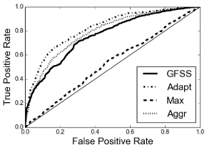
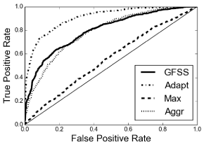
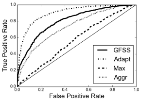
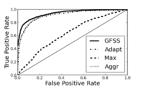
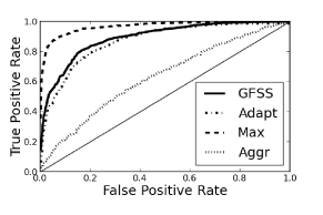
In the first experiment (Figure 2 left), we chose 333 aquifers at random which resulted in 112112112 contaminated wells. By our choice of โ€–๐ฑโ€–2=5superscriptnorm๐ฑ25\|\mathbf{x}\|^{2}=5, the signal size at each contaminated well was 0.470.470.47 which is substantially less than the noise level ฯƒ๐œŽ\sigma. In the second experiment (Figure 2 middle), we chose 111 of the larger aquifers (with greater than 100100100 wells) at random which resulted in 109109109 contaminated wells. In the third experiment (Figure 2 right), we selected 111 of the somewhat smaller aquifer (with greater than 505050 wells) at random which resulted in 626262 contaminated wells. We simulate the probability of correct detection (rejecting H0subscript๐ป0H_{0} when the truth is H1subscript๐ป1H_{1}) versus the probability of false alarm (falsely rejecting H0subscript๐ป0H_{0}) by making 100010001000 draws from the noise distribution (with and without the signal ๐ฑ๐ฑ\mathbf{x} for H1subscript๐ป1H_{1} and H0subscript๐ป0H_{0} respectively).

Refer to caption
Refer to caption
Refer to caption
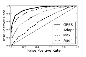
Figure 2: (Arsenic Contamination Simulations) Simulations of the size (false positive rate) and the power under H1Pโ€‹Csuperscriptsubscript๐ป1๐‘ƒ๐ถH_{1}^{PC} for the As simulations of the GFSS, adaptive GFSS (Adapt), Max statistic (Max), and Aggregate statistic (Aggr). The figures are for 3 contaminated aquifers (left), 1 large contaminated aquifer (middle), and 1 smaller contaminated aquifer (right).

As can be seen the adaptive GFSS test strictly outperforms all of the test statistics, which demonstrates the importance of adapting to the ฯ๐œŒ\rho parameter. Moreover, the GFSS with the somewhat arbitrary choice of ฯ=ฮป109๐œŒsubscript๐œ†109\rho=\lambda_{109} begins to outperform the Aggregate statistic for the smaller contamination as our theory predicts. The adaptive GFSS is a substantially better alternative to an arbitrary choice of ฯ๐œŒ\rho and statistics that do not take the kNN graph structure into account.

While Theorem 9 can be inverted to obtain a P-value that is valid for finite p๐‘p, this may be too conservative for practical purposes. We recommend one of two approaches: forming a Z-score that is asymptotically normal under H0subscript๐ป0H_{0}, and using a permutation test. Under H0subscript๐ป0H_{0}, the GFSS, t^^๐‘ก\hat{t}, has zero mean and because it is the sum of weighted ฯ‡12subscriptsuperscript๐œ’21\chi^{2}_{1} random variables it has a variance of 2โ€‹(โˆ‘i=2phโ€‹(ฮปi)4)2superscriptsubscript๐‘–2๐‘โ„Žsuperscriptsubscript๐œ†๐‘–42(\sum_{i=2}^{p}h(\lambda_{i})^{4}). Thus, a Z-score can be calculated by Z^=t^/2โ€‹โˆ‘i=2phโ€‹(ฮปi)4^๐‘^๐‘ก2superscriptsubscript๐‘–2๐‘โ„Žsuperscriptsubscript๐œ†๐‘–4\hat{Z}=\hat{t}/\sqrt{2\sum_{i=2}^{p}h(\lambda_{i})^{4}}, which can be shown to have an asymptotic standard normal distribution under some regularity conditions. Thus, we can form an asymptotically valid P-value by applying the standard normal inverse CDF to Z^^๐‘\hat{Z}. While this is valid when the noise is Gaussian, in many instances the measurements are not Gaussian and we interpret H0subscript๐ป0H_{0} to mean that xi=๐”ผโ€‹yisubscript๐‘ฅ๐‘–๐”ผsubscript๐‘ฆ๐‘–x_{i}=\mathbb{E}y_{i} is constant over the graph which is a weaker assumption (recall we had binary observations in section I.A, but we used the GFSS none-the-less). In this case, we can apply a permutation test, by which we randomly permute the coordinates of ๐ฒ๐ฒ\mathbf{y} and maintain the graph structure. We interpret the resulting statistic t^^๐‘ก\hat{t} as a simulation of the GFSS under H0subscript๐ป0H_{0}. Then an estimated P-value would be the fraction of permutations that have a larger t^^๐‘ก\hat{t} then the actual GFSS. This was used to construct the reported P-values in Section I.B.

6.B Balanced Binary Trees

Balanced trees are graph structures of particular interest because they provide a simple hierarchical structure. Furthermore, the behavior of the graph spectra for the balanced binary tree provides a natural multiscale basis [SNC10, SS10]. We begin this analysis of the GFSS by applying it to the balanced binary tree (BBT) of depth โ„“โ„“\ell. We consider the class of signals defined by ฯ=[cโ€‹pฮฑโ€‹(1โˆ’cโ€‹pฮฑโˆ’1)]โˆ’1๐œŒsuperscriptdelimited-[]๐‘superscript๐‘๐›ผ1๐‘superscript๐‘๐›ผ11\rho=[cp^{\alpha}(1-cp^{\alpha-1})]^{-1} where 0<cโ‰ค1/2,0<ฮฑโ‰ค1formulae-sequence0๐‘120๐›ผ10<c\leq 1/2,0<\alpha\leq 1. This class is interesting as it includes, among others, clusters of constant signal which are subtrees of size at least cโ€‹pฮฑ๐‘superscript๐‘๐›ผcp^{\alpha} (subtrees can be isolated from a tree by cutting a single edge and hence have cut size 111).

Corollary 15.

Let G๐บG be a balanced binary tree with p๐‘p vertices, and let ฯ=pโ€‹[cโ€‹pฮฑโ€‹(pโˆ’cโ€‹pฮฑ)]โˆ’1๐œŒ๐‘superscriptdelimited-[]๐‘superscript๐‘๐›ผ๐‘๐‘superscript๐‘๐›ผ1\rho=p[cp^{\alpha}(p-cp^{\alpha})]^{-1}.
(a) The GFSS can asymptotically distinguish H0subscript๐ป0H_{0} from signals within H1Pโ€‹C,H1Ssuperscriptsubscript๐ป1๐‘ƒ๐ถsuperscriptsubscript๐ป1๐‘†H_{1}^{PC},H_{1}^{S} if the SNR is stronger than

ฮผฯƒ=ฯ‰โ€‹(p1โˆ’ฮฑ4โ€‹(logโกp)1/4).๐œ‡๐œŽ๐œ”superscript๐‘1๐›ผ4superscript๐‘14\frac{\mu}{\sigma}=\omega(p^{\frac{1-\alpha}{4}}(\log p)^{1/4}).

(b) The adaptive GFSS distinguishes the hypotheses of (a) if

ฮผฯƒ=ฯ‰โ€‹(p1โˆ’ฮฑ4โ€‹(logโกp)1/2).๐œ‡๐œŽ๐œ”superscript๐‘1๐›ผ4superscript๐‘12\frac{\mu}{\sigma}=\omega(p^{\frac{1-\alpha}{4}}(\log p)^{1/2}).

(c) H0subscript๐ป0H_{0} and H1Pโ€‹Csuperscriptsubscript๐ป1๐‘ƒ๐ถH_{1}^{PC} are asymptotically indistinguishable if

ฮผฯƒ=oโ€‹(p1โˆ’ฮฑ4).๐œ‡๐œŽ๐‘œsuperscript๐‘1๐›ผ4\frac{\mu}{\sigma}=o(p^{\frac{1-\alpha}{4}}).

The conclusion is that for the BBT the GFSS and the adaptive GFSS is near optimal with respect to critical SNR. The proof (Appendix A) is based on the special form of the spectrum of the BBT. So in this case, the GFSS consistently dominates the naive statistics and the theoretical results are very close to the lower bounds for any ฮฑ๐›ผ\alpha.

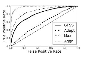
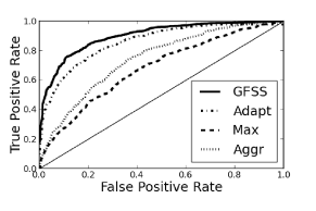
We simulate the probability of correct detection versus the probability of false alarm. These are given for the four statistics in Figure 3 as the test threshold, and hence the probability of false alarm, is varied. The GFSS is computed with the correct ฯ๐œŒ\rho, which is in general unknown. Different statistics dominate under different choices of cluster size parameter, ฮฑ๐›ผ\alpha. When ฮฑ=1๐›ผ1\alpha=1, corresponding to large clusters, where the size is on the same order as p๐‘p, the aggregate statistic is competitive with the adaptive statistic. When ฮฑ=0.5๐›ผ0.5\alpha=0.5, corresponding to clusters of size โ‰p1/2asymptotically-equalsabsentsuperscript๐‘12\asymp p^{1/2}, the aggregate becomes less competitive and the max more competitive than the ฮฑ=1๐›ผ1\alpha=1 case, and the GFSS remains the dominating test. In each case, we set c=1/2๐‘12c=1/2, which ensures that the ฮฑ=1๐›ผ1\alpha=1 case does not select the entire tree.
Refer to caption
Refer to caption
Figure 3: (BBT Comparisons) Simulations of the size (false positive rate) and the power under H1Pโ€‹Csuperscriptsubscript๐ป1๐‘ƒ๐ถH_{1}^{PC} for the balanced binary tree of the GFSS, adaptive GFSS (Adapt), Max statistic (Max), and Aggregate statistic (Aggr). The figures are for the tree of depth โ„“=6โ„“6\ell=6, p=2โ„“+1โˆ’1=127๐‘superscript2โ„“11127p=2^{\ell+1}-1=127, with choice of ฮฑ=1๐›ผ1\alpha=1 (left) and ฮฑ=0.5๐›ผ0.5\alpha=0.5 (right).

6.C Torus Graph

The torus has been a pedagogical example, but it is also an important example as it models a mesh of sensors in two dimensions. We will analyze the performance guarantees of the GFSS over our running example, the 2-dimensional torus graph with โ„“โ„“\ell vertices along each dimension (p=โ„“2๐‘superscriptโ„“2p=\ell^{2}). To include squares of size p1โˆ’ฮฒsuperscript๐‘1๐›ฝp^{1-\beta}, as in the examples, then we would obtain ฯโ‰pโˆ’(1โˆ’ฮฒ)/2asymptotically-equals๐œŒsuperscript๐‘1๐›ฝ2\rho\asymp p^{-(1-\beta)/2}. The following result is due to a detailed analysis of the spectrum of the torus.

Corollary 16.

Let G๐บG be the โ„“ร—โ„“โ„“โ„“\ell\times\ell square torus (p=โ„“2๐‘superscriptโ„“2p=\ell^{2}), and let ฯ=cโ€‹pโˆ’(1โˆ’ฮฒ)/2๐œŒ๐‘superscript๐‘1๐›ฝ2\rho=cp^{-(1-\beta)/2} for ฮฒโˆˆ[0,1)๐›ฝ01\beta\in[0,1).
(a) The GFSS can asymptotically distinguish H0subscript๐ป0H_{0} from H1Pโ€‹C,H1Ssuperscriptsubscript๐ป1๐‘ƒ๐ถsuperscriptsubscript๐ป1๐‘†H_{1}^{PC},H_{1}^{S} if the SNR satisfies

ฮผฯƒ=ฯ‰โ€‹(p320+110โ€‹ฮฒ).๐œ‡๐œŽ๐œ”superscript๐‘320110๐›ฝ\frac{\mu}{\sigma}=\omega(p^{\frac{3}{20}+\frac{1}{10}\beta}).

(b) The adaptive GFSS can asymptotically distinguish the hypotheses of (a) if

ฮผฯƒ=ฯ‰โ€‹(p320+110โ€‹ฮฒโ€‹(logโกp)1/4).๐œ‡๐œŽ๐œ”superscript๐‘320110๐›ฝsuperscript๐‘14\frac{\mu}{\sigma}=\omega(p^{\frac{3}{20}+\frac{1}{10}\beta}(\log p)^{1/4}).

(c) H0subscript๐ป0H_{0} and H1Pโ€‹Csuperscriptsubscript๐ป1๐‘ƒ๐ถH_{1}^{PC} are asymptotically indistinguishable if the SNR is weaker than

ฮผฯƒ=oโ€‹(pฮฒ4).๐œ‡๐œŽ๐‘œsuperscript๐‘๐›ฝ4\frac{\mu}{\sigma}=o(p^{\frac{\beta}{4}}).

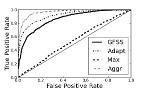
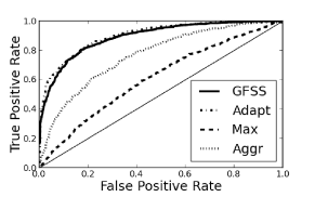
The implication of Cor.ย 16 is that when ฮฒ>0๐›ฝ0\beta>0 (the clusters are not too large), the GFSS is consistent under an SNR lower than p1/4superscript๐‘14p^{1/4}. Regardless of the ฮฒ๐›ฝ\beta parameter the GFSS never achieves the lower bound for the torus graph, which suggests an approach that exploits the specific structure of the torus may yet outperform the GFSS. We simulate the performance of the test statistics over a 30ร—30303030\times 30 torus, with ฮฒ=0,.5,.75๐›ฝ0.5.75\beta=0,.5,.75 with c=1/2๐‘12c=1/2 When ฮฒ๐›ฝ\beta is small (large clusters), we suffer an additional factor of p3โ€‹(1โˆ’ฮฒ)/20superscript๐‘31๐›ฝ20p^{3(1-\beta)/20} in the upper bound. Despite the theoretical shortcomings of in this case, the simulations (Figure 4) suggest that the GFSS is significantly superior to the naive tests for medium sized clusters.
Refer to caption
Refer to caption
Refer to caption
Figure 4: (Torus Comparisons) Simulations of the size (false positive rate) and the power under H1Pโ€‹Csuperscriptsubscript๐ป1๐‘ƒ๐ถH_{1}^{PC} for the Torus of the GFSS, adaptive GFSS (Adapt), Max statistic (Max), and Aggregate statistic (Aggr). The figures are for side length of โ„“=30โ„“30\ell=30, p=โ„“2=900๐‘superscriptโ„“2900p=\ell^{2}=900, with choice of ฮฒ=0๐›ฝ0\beta=0 (top left), ฮฒ=.5๐›ฝ.5\beta=.5 (top right) and ฮฒ=.75๐›ฝ.75\beta=.75 (bottom).

6.D Kronecker Graphs

Much of the research in complex networks has focused on observing statistical phenomena that is common across many data sources. The most notable of these are that the degree distribution obeys a power law ([FFF99]) and networks are often found to have small diameter ([Mil67]). A class of graphs that satisfy these, while providing a simple modelling platform are the Kronecker graphs (see [LF07, LCK+10]). Let H1subscript๐ป1H_{1} and H2subscript๐ป2H_{2} be graphs on p0subscript๐‘0p_{0} vertices with Laplacians ฮ”1,ฮ”2subscriptฮ”1subscriptฮ”2\Delta_{1},\Delta_{2} and edge sets E1,E2subscript๐ธ1subscript๐ธ2E_{1},E_{2} respectively. The Kronecker product, H1โŠ—H2tensor-productsubscript๐ป1subscript๐ป2H_{1}\otimes H_{2}, is the graph over vertices [p0]ร—[p0]delimited-[]subscript๐‘0delimited-[]subscript๐‘0[p_{0}]\times[p_{0}] such that there is an edge ((i1,i2),(j1,j2))subscript๐‘–1subscript๐‘–2subscript๐‘—1subscript๐‘—2((i_{1},i_{2}),(j_{1},j_{2})) if i1=j1subscript๐‘–1subscript๐‘—1i_{1}=j_{1} and (i2,j2)โˆˆE2subscript๐‘–2subscript๐‘—2subscript๐ธ2(i_{2},j_{2})\in E_{2} or i2=j2subscript๐‘–2subscript๐‘—2i_{2}=j_{2} and (i1,j1)โˆˆE1subscript๐‘–1subscript๐‘—1subscript๐ธ1(i_{1},j_{1})\in E_{1}. We will construct graphs that have a multi-scale topology using the Kronecker product. Let the multiplication of a graph by a scalar indicate that we multiply each edge weight by that scalar. First let H๐ปH be a connected graph with p0subscript๐‘0p_{0} vertices. Then the graph G๐บG for โ„“>0โ„“0\ell>0 levels is defined as

1p0โ„“โˆ’1โ€‹HโŠ—1p0โ„“โˆ’2โ€‹HโŠ—โ€ฆโŠ—1p0โ€‹HโŠ—H.tensor-producttensor-producttensor-product1superscriptsubscript๐‘0โ„“1๐ป1superscriptsubscript๐‘0โ„“2๐ปโ€ฆ1subscript๐‘0๐ป๐ป\frac{1}{p_{0}^{\ell-1}}H\otimes\frac{1}{p_{0}^{\ell-2}}H\otimes...\otimes\frac{1}{p_{0}}H\otimes H.

The choice of multipliers ensures that it is easier to make cuts at the more coarse scale. Notice that all of the previous results have held for weighted graphs.

Corollary 17.

Let G๐บG be the Kronecker product of the base graph H๐ปH described above with p=p0โ„“๐‘superscriptsubscript๐‘0โ„“p=p_{0}^{\ell} vertices, and let ฯโ‰p02โ€‹kโˆ’โ„“โˆ’1asymptotically-equals๐œŒsuperscriptsubscript๐‘02๐‘˜โ„“1\rho\asymp p_{0}^{2k-\ell-1} (which includes cuts within the k๐‘˜k coarsest scale).
(a) The GFSS can asymptotically distinguish H0subscript๐ป0H_{0} from signals from H1Pโ€‹C,H1Ssuperscriptsubscript๐ป1๐‘ƒ๐ถsuperscriptsubscript๐ป1๐‘†H_{1}^{PC},H_{1}^{S} if the SNR is stronger than

ฮผฯƒ=ฯ‰โ€‹(pk/2โ€‹โ„“โ€‹(diamโ€‹(H))1/4),๐œ‡๐œŽ๐œ”superscript๐‘๐‘˜2โ„“superscriptdiam๐ป14\frac{\mu}{\sigma}=\omega(p^{k/2\ell}(\textrm{diam}(H))^{1/4}),

where diamโ€‹(H)diam๐ป\textrm{diam}(H) is the diameter of the base graph H๐ปH.
(b) The adaptive GFSS can distinguish the hypotheses of (a) if

ฮผฯƒ=ฯ‰โ€‹(pk/2โ€‹โ„“โ€‹(diamโ€‹(H)โ€‹logโกp)1/4).๐œ‡๐œŽ๐œ”superscript๐‘๐‘˜2โ„“superscriptdiam๐ป๐‘14\frac{\mu}{\sigma}=\omega(p^{k/2\ell}(\textrm{diam}(H)\log p)^{1/4}).

(c) H0subscript๐ป0H_{0} and H1Pโ€‹Csuperscriptsubscript๐ป1๐‘ƒ๐ถH_{1}^{PC} are asymptotically indistinguishable if

ฮผฯƒ=oโ€‹(pk/4โ€‹โ„“).๐œ‡๐œŽ๐‘œsuperscript๐‘๐‘˜4โ„“\frac{\mu}{\sigma}=o(p^{k/4\ell}).

The proof and an explanation of ฯ๐œŒ\rho is in the appendix. The implication of Cor.ย 17 is that only for k๐‘˜k small is the GFSS nearly optimal. Generally, one will suffer a multiplicative term of pk/4โ€‹โ„“superscript๐‘๐‘˜4โ„“p^{k/4\ell}. As we can see from the simulations the k=1๐‘˜1k=1 case is exactly when the aggregate statistic dominates (see Figure 5). When 1<k<โ„“1๐‘˜โ„“1<k<\ell, the GFSS improves on the aggregate and the max statistics. Throughout these simulations we set ฯ=p02โ€‹kโˆ’โ„“โˆ’1๐œŒsuperscriptsubscript๐‘02๐‘˜โ„“1\rho=p_{0}^{2k-\ell-1}.

Refer to caption
Refer to caption
Figure 5: (Kronecker Comparison) Simulations of the size (false positive rate) and the power under H1Pโ€‹Csuperscriptsubscript๐ป1๐‘ƒ๐ถH_{1}^{PC} for the Kronecker graph of the GFSS, adaptive GFSS (Adapt), Max statistic (Max), and Aggregate statistic (Aggr). The figures are for a base graph of size p0=6subscript๐‘06p_{0}=6 and Kronecker power of โ„“=3โ„“3\ell=3, so p=p0โ„“=216๐‘superscriptsubscript๐‘0โ„“216p=p_{0}^{\ell}=216. The cuts were chosen at the coarsest scale, k=1๐‘˜1k=1, (left) and at the second coarsest, k=2๐‘˜2k=2 (right).

One may rightly ask if the gap between the upper bounds (Corollaries 15 (b), 16 (b), 17 (b)) and the lower bounds (Corollaries 15 (c), 16 (c), 17 (c)) is just due to a lack of theoretical know-how and the test is actually optimal. We attempt to assess this concern by plotting the performance of the GFSS with the SNR increasing according to the scaling dictated by the upper bounds (Figure 6). For the BBT because the curve does not change significantly with p๐‘p (as the tree depth l๐‘™l increases), the upper bound is supposed to be tight. In the torus graph, for large rectangles (ฮฒ=0๐›ฝ0\beta=0) the upper bound appears to be correct, while for moderately sized rectangles (ฮฒ=.5๐›ฝ.5\beta=.5) there may be a gap between our theoretical bound, 16 (b), and the actual performance of GFSS. For the Kronecker graph there appears to be a gap for both scalings (k=1๐‘˜1k=1 and k=2๐‘˜2k=2) of cluster size, indicating that the performance of the GFSS may be better than predicted by our theory.
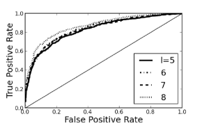
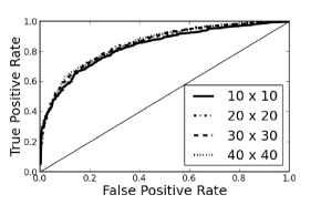
Refer to caption
Refer to caption
Refer to caption
Refer to caption
Refer to caption
Refer to caption
Figure 6: (Rescaling by Theoretical Bounds) The size (false positive rate) and power (true positive rate) of the GFSS as p๐‘p increases for the following graph and signal models: BBT with ฮฑ=1๐›ผ1\alpha=1 (top left) and ฮฑ=.5๐›ผ.5\alpha=.5 (bottom left); Torus with ฮฒ=0๐›ฝ0\beta=0 (top middle) and ฮฒ=.5๐›ฝ.5\beta=.5 (bottom middle); Kronecker graph with base graph size p0=6subscript๐‘06p_{0}=6 and k=1๐‘˜1k=1 (top right) and k=2๐‘˜2k=2 (bottom right). The SNR was allowed to scale according to Cor.ย 15 (b) (left), Cor.ย 16 (b) (middle), Cor.ย 17 (b) (right).

6.E General Graph Structure, H1Ssuperscriptsubscript๐ป1๐‘†H_{1}^{S}

The piecewise constant alternative hypothesis H1Pโ€‹Csuperscriptsubscript๐ป1๐‘ƒ๐ถH_{1}^{PC} is amenable to a sophisticated theoretical analysis and it motivates the GFSS. Unfortunately, it is very easy to modify signals in ๐’ณPโ€‹Cโ€‹(ฮผ,ฯ)subscript๐’ณ๐‘ƒ๐ถ๐œ‡๐œŒ\mathcal{X}_{PC}(\mu,\rho) by slight perturbations and find a signal that is outside our supposed class. This lack of robustness is rightly alarming, and it is through the general graph structured class, ๐’ณSโ€‹(ฮผ,ฯ)subscript๐’ณ๐‘†๐œ‡๐œŒ\mathcal{X}_{S}(\mu,\rho), that we intended to include these perturbations. We now provide a signal subsampling scheme that will demonstrate the performance of the GFSS under signal perturbations.

Suppose that we begin with a signal ๐ฑโˆˆ๐’ณPโ€‹Cโ€‹(ฮผ,ฯ)๐ฑsubscript๐’ณ๐‘ƒ๐ถ๐œ‡๐œŒ\mathbf{x}\in\mathcal{X}_{PC}(\mu,\rho) such that ๐ฑ=ฮดโ€‹๐ŸC๐ฑ๐›ฟsubscript1๐ถ\mathbf{x}=\delta{\bf 1}_{C} and modify it in the following way: let Cโ€ฒโŠ‚Csuperscript๐ถโ€ฒ๐ถC^{\prime}\subset C and make ๐ฑโ€ฒโˆ๐ŸCโ€ฒproportional-tosuperscript๐ฑโ€ฒsuperscriptsubscript1๐ถโ€ฒ\mathbf{x}^{\prime}\propto{\bf 1}_{C}^{\prime} such that ๐ฑโ€ฒโˆˆ๐’ณSโ€‹(ฮผ,ฯ)superscript๐ฑโ€ฒsubscript๐’ณ๐‘†๐œ‡๐œŒ\mathbf{x}^{\prime}\in\mathcal{X}_{S}(\mu,\rho). We now determine the normalization that would make this so. Notice that

|๐ฑโ€ฒโฃโŠคโ€‹๐ŸC|C|โˆ’๐ฑโ€ฒโฃโŠคโ€‹๐ŸCยฏ|Cยฏ||โ€‹|C|โ€‹|Cยฏ|pโ‰ฅฮผ.superscript๐ฑโ€ฒtopsubscript1๐ถ๐ถsuperscript๐ฑโ€ฒtopsubscript1ยฏ๐ถยฏ๐ถ๐ถยฏ๐ถ๐‘๐œ‡\left|\frac{\mathbf{x}^{\prime\top}{\bf 1}_{C}}{|C|}-\frac{\mathbf{x}^{\prime\top}{\bf 1}_{\bar{C}}}{|\bar{C}|}\right|\sqrt{\frac{|C||\bar{C}|}{p}}\geq\mu.

Hence, ๐ฑโ€ฒ=ฮดโ€ฒโ€‹๐ŸCโ€ฒsuperscript๐ฑโ€ฒsuperscript๐›ฟโ€ฒsubscript1superscript๐ถโ€ฒ\mathbf{x}^{\prime}=\delta^{\prime}{\bf 1}_{C^{\prime}} implies that ฮดโ€ฒ=ฮดโ€‹|C|/|Cโ€ฒ|superscript๐›ฟโ€ฒ๐›ฟ๐ถsuperscript๐ถโ€ฒ\delta^{\prime}=\delta|C|/|C^{\prime}| is sufficient. So for the subsampled signal ๐ฑโ€ฒsuperscript๐ฑโ€ฒ\mathbf{x}^{\prime} to remain in ๐’ณSโ€‹(ฮผ,ฯ)subscript๐’ณ๐‘†๐œ‡๐œŒ\mathcal{X}_{S}(\mu,\rho) we will need to boost the signal by a factor of |C|/|Cโ€ฒ|๐ถsuperscript๐ถโ€ฒ|C|/|C^{\prime}|. Figure 7 shows the performance curves for the GFSS when the signal cluster Cโ€ฒsuperscript๐ถโ€ฒC^{\prime} is formed by including each vertex in C๐ถC according to independent Bernoulli(q๐‘žq) random variables for the BBT. To make the comparison fair we boost the signal according to the above formulation. As one can see the subsampling does not make the performance worse.
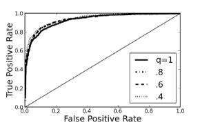
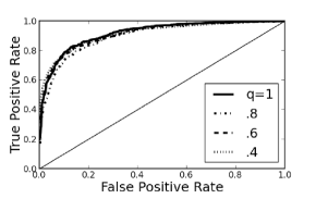
Refer to caption
Refer to caption
Figure 7: (BBT Perturbations) Simulations of the size (false positive rate) and the power under H1Ssuperscriptsubscript๐ป1๐‘†H_{1}^{S} for the balanced binary tree of the GFSS with changing cluster sampling probability, q๐‘žq. The figures are for the tree of depth โ„“=6โ„“6\ell=6, p=2โ„“+1โˆ’1=127๐‘superscript2โ„“11127p=2^{\ell+1}-1=127, with choice of ฮฑ=1๐›ผ1\alpha=1 (left) and ฮฑ=0.5๐›ผ0.5\alpha=0.5 (right).

7 Conclusion

We studied the problem of how to tractably detect anomalous activities in networks under Gaussian noise. We outlined what is known regarding the performance of the agglomerative and maximum statistics. These statistics do not take into account the graph structure and we wish instead to exploit the structure of the graph to obtain a superior test statistic. To this end we developed the graph Fourier scan statistic, suggesting it as a computationally feasible alternative to the GLRT. We completely characterized the performance of the GFSS for any graph in terms of the spectrum of the combinatorial Laplacian. The theoretical analysis of the GFSS naturally led to the development of the adaptive GFSS.

We applied the main result to three graph models: balanced binary trees, the lattice and Kronecker graph. We demonstrated that the performance is not specific to piecewise constant signals, and we are able to extend our results to a more general alternative class, H1Ssuperscriptsubscript๐ป1๐‘†H_{1}^{S}. We demonstrated that though the theoretical performance of the GFSS for the Torus graph and Kronecker graph may be sub-optimal, there is experimental evidence to indicate that this is partly an artifact of the theoretical analysis technique. We see that not only is it statistically sub-optimal to ignore graph structure, but in many of these cases the GFSS gives a near optimal performance.

References

  • [ABBDL10] L.ย Addario-Berry, N.ย Broutin, L.ย Devroye, and G.ย Lugosi. On combinatorial testing problems. The Annals of Statistics, 38(5):3063โ€“3092, 2010.
  • [ACCD11] E.ย Arias-Castro, E.J. Candes, and A.ย Durand. Detection of an anomalous cluster in a network. The Annals of Statistics, 39(1):278โ€“304, 2011.
  • [ACCHZ08] E.ย Arias-Castro, E.J. Candes, H.ย Helgason, and O.ย Zeitouni. Searching for a trail of evidence in a maze. The Annals of Statistics, 36(4):1726โ€“1757, 2008.
  • [ACDH05] E.ย Arias-Castro, D.ย Donoho, and X.ย Huo. Near-optimal detection of geometric objects by fast multiscale methods. IEEE Trans. Inform. Theory, 51(7):2402โ€“2425, 2005.
  • [BH95] B.ย Baygรผn and A.ย O. Hero. Optimal simultaneous detection and estimation under a false alarm constraint. Signal Processing, IEEE Transactions on, 41(3):688โ€“703, 1995.
  • [BN01] Mikhail Belkin and Partha Niyogi. Laplacian eigenmaps and spectral techniques for embedding and clustering. In NIPS, volumeย 14, pages 585โ€“591, 2001.
  • [BXKS11] Sivaraman Balakrishnan, Min Xu, Akshay Krishnamurthy, and Aarti Singh. Noise thresholds for spectral clustering. In Advances in Neural Information Processing Systems, pages 954โ€“962, 2011.
  • [CM06] Ronaldย R Coifman and Mauro Maggioni. Diffusion wavelets. Applied and Computational Harmonic Analysis, 21(1):53โ€“94, 2006.
  • [FFF99] M.ย Faloutsos, P.ย Faloutsos, and C.ย Faloutsos. On power-law relationships of the internet topology. In ACM SIGCOMM Computer Communication Review, volumeย 29, pages 251โ€“262. ACM, 1999.
  • [FFN08] M.ย Fouladirad, L.ย Freitag, and I.ย Nikiforov. Optimal fault detection with nuisance parameters and a general covariance matrix. International Journal of Adaptive Control and Signal Processing, 22(5):431โ€“439, 2008.
  • [Fie75] M.ย Fiedler. Eigenvectors of acyclic matrices. Czechoslovak Mathematical Journal, 25(4):607โ€“618, 1975.
  • [Fil12] L.ย Fillatre. Asymptotically uniformly minimax detection and isolation in network monitoring. to appear in Signal Processing, IEEE Transactions on, 2012.
  • [FN05] M.ย Fouladirad and I.ย Nikiforov. Optimal statistical fault detection with nuisance parameters. Automatica, 41(7):1157โ€“1171, 2005.
  • [FWW+99] MJย Focazio, AHย Welch, SAย Watkins, DRย Helsel, and MAย Horn. A retrospective analysis on the occurrence of arsenic in ground-water resources of the united states and limitations in drinking-water-supply characterizations: Us geological survey water-resources investigation report 99-4279, 1999. Washington, DC, USA, 1999.
  • [HKTP98] Wolfgang Hรคrdle, Gerard Kerkyacharian, Alexander Tsybakov, and Dominique Picard. Wavelets, approximation, and statistical applications. Springer, 1998.
  • [HVG11] Davidย K Hammond, Pierre Vandergheynst, and Rรฉmi Gribonval. Wavelets on graphs via spectral graph theory. Applied and Computational Harmonic Analysis, 30(2):129โ€“150, 2011.
  • [IS03] Y.I. Ingster and I.A. Suslina. Nonparametric goodness-of-fit testing under Gaussian models, volume 169. Springer Verlag, 2003.
  • [JN12] P.ย Ji and M.ย Nussbaum. Sharp adaptive nonparametric testing for sobolev ellipsoids. arXiv preprint arXiv:1210.8162, 2012.
  • [KMP10] Ioannis Koutis, Garyย L Miller, and Richard Peng. Approaching optimality for solving sdd linear systems. In Foundations of Computer Science (FOCS), 2010 51st Annual IEEE Symposium on, pages 235โ€“244. IEEE, 2010.
  • [LCK+10] J.ย Leskovec, D.ย Chakrabarti, J.ย Kleinberg, C.ย Faloutsos, and Z.ย Ghahramani. Kronecker graphs: An approach to modeling networks. The Journal of Machine Learning Research, 11:985โ€“1042, 2010.
  • [LF07] J.ย Leskovec and C.ย Faloutsos. Scalable modeling of real graphs using kronecker multiplication. In Proceedings of the 24th international conference on Machine learning, pages 497โ€“504. ACM, 2007.
  • [LM00] B.ย Laurent and P.ย Massart. Adaptive estimation of a quadratic functional by model selection. The annals of Statistics, 28(5):1302โ€“1338, 2000.
  • [LR05] E.L. Lehmann and J.P. Romano. Testing statistical hypotheses. Springer Verlag, 2005.
  • [Mer98] R.ย Merris. Laplacian graph eigenvectors. Linear algebra and its applications, 278(1):221โ€“236, 1998.
  • [Mil67] S.ย Milgram. The small world problem. Psychology today, 2(1):60โ€“67, 1967.
  • [MNS00] J.J. Molitierno, M.ย Neumann, and B.L. Shader. Tight bounds on the algebraic connectivity of a balanced binary tree. Electronic Journal of Linear Algebra, 6:62โ€“71, 2000.
  • [Mur07] F.ย Murtagh. The haar wavelet transform of a dendrogram. Journal of Classification, 24:3โ€“32, 2007.
  • [NJW+02] Andrewย Y Ng, Michaelย I Jordan, Yair Weiss, etย al. On spectral clustering: Analysis and an algorithm. Advances in neural information processing systems, 2:849โ€“856, 2002.
  • [NSJ07] Jens Nilsson, Fei Sha, and Michaelย I Jordan. Regression on manifolds using kernel dimension reduction. In Proceedings of the 24th international conference on Machine learning, pages 697โ€“704. ACM, 2007.
  • [Pri04] Careyย E. Priebe. Scan statistics on graphs. Technical Report 650, Johns Hopkins University, Baltimore, MD 21218-2682, 2004.
  • [Roj02] O.ย Rojo. The spectrum of the laplacian matrix of a balanced binary tree. Linear algebra and its applications, 349(1):203โ€“219, 2002.
  • [RS05] O.ย Rojo and R.ย Soto. The spectra of the adjacency matrix and laplacian matrix for some balanced trees. Linear algebra and its applications, 403:97โ€“117, 2005.
  • [SF94] L.ย L. Scharf and B.ย Friedlander. Matched sub-space detectors. Signal Processing, IEEE Transactions on, 42(8):2146โ€“2157, 1994.
  • [SKS13a] James Sharpnack, Akshay Krishnamurthy, and Aarti Singh. Detecting activations over graphs using spanning tree wavelet bases. In Artifical Intelligence and Statistics (AISTATS), 2013.
  • [SKS13b] James Sharpnack, Akshay Krishnamurthy, and Aarti Singh. Near-optimal anomaly detection in graphs using lovรกsz extended scan statistic. Submitted, 2013.
  • [SM14] Aliaksei Sandryhaila and Jย Moura. Discrete signal processing on graphs. Transactions on Signal Processing, 60, 2014.
  • [SN10] Skyler Speakman and Danielย B. Neill. Fast graph scan for scalable detection of arbitrary connected clusters. In Proceedings of the 2009 International Society for Disease Surveillance Annual Conference, 2010.
  • [SNC10] Aarti Singh, Robertย D Nowak, and Robert Calderbank. Detecting weak but hierarchically-structured patterns in networks. arXiv preprint arXiv:1003.0205, 2010.
  • [SNF+13] D.I. Shuman, S.K. Narang, P.ย Frossard, A.ย Ortega, and P.ย Vandergheynst. The emerging field of signal processing on graphs: Extending high-dimensional data analysis to networks and other irregular domains. IEEE Signal Processing Magazine, 30(3):83โ€“98, 2013.
  • [Spo96] V.G. Spokoiny. Adaptive hypothesis testing using wavelets. The Annals of Statistics, 24(6):2477โ€“2498, 1996.
  • [SRS13] James Sharpnack, Alessandro Rinaldo, and Aarti Singh. Changepoint detection over graphs with the spectral scan statistic. AIStats (JMLR WCP), 2013.
  • [SS10] J.ย Sharpnack and A.ย Singh. Identifying graph-structured activation patterns in networks. In Proceedings of Neural Information Processing Systems, NIPS, 2010.
  • [SS13] James Sharpnack and Aarti Singh. Near-optimal and computationally efficient detectors for weak and sparse graph-structured patterns. In IEEE Global Conference on Signal and Information Processing, 2013.
  • [USG03] Principal aquifers of the 48 conterminous united states, hawaii, puerto rico, and the u.s. virgin islands. http://water.usgs.gov/lookup/getspatial?aquifers_us, 2003.
  • [Vaz01] Vijayย V Vazirani. Approximation algorithms. springer, 2001.
  • [Wal43] A.ย Wald. Tests of statistical hypotheses concerning several parameters when the number of observations is large. Transactions of American Mathematical Society, 54:426โ€“482, 1943.

Appendix A Proofs

The result now follows by considering all the indicator functions corresponding to the sets in ๐’ž๐’ž\mathcal{C}.

Proof of Proposition 8.

To prove the claim we will first rewrite the SSS in an equivalent but more convenient form which we will then bound from above and below using the GFSS. To this end we recall the arguments from Lemma 7 of [SRS13]. Since G๐บG is connected, the combinatorial Laplacian ฮ”ฮ”\Delta is symmetric, its smallest eigenvalue is zero and the remaining eigenvalues are positive. By the spectral theorem, we can write ฮ”=๐”โ€‹ฮ›โ€‹๐”โŠคฮ”๐”ฮ›superscript๐”top\Delta=\mathbf{U}\Lambda\mathbf{U}^{\top}, where ฮ›ฮ›\Lambda is a (pโˆ’1)ร—(pโˆ’1)๐‘1๐‘1(p-1)\times(p-1) diagonal matrix containing the positive eigenvalues of ฮ”ฮ”\Delta, ฮป2,โ€ฆ,ฮปpsubscript๐œ†2โ€ฆsubscript๐œ†๐‘\lambda_{2},\ldots,\lambda_{p}, in increasing order. The columns of the pร—(pโˆ’1)๐‘๐‘1p\times(p-1) matrix ๐”๐”\mathbf{U} are the associated eigenvectors. Then, since each vector ๐ฑโˆˆโ„p๐ฑsuperscriptโ„๐‘\mathbf{x}\in\mathbb{R}^{p} with ๐ŸโŠคโ€‹๐ฑ=0superscript1top๐ฑ0{\bf 1}^{\top}\mathbf{x}=0 can be written as ๐”๐ณ๐”๐ณ\mathbf{U}\mathbf{z} for a unique vector ๐ณโˆˆโ„pโˆ’1๐ณsuperscriptโ„๐‘1\mathbf{z}\in\mathbb{R}^{p-1}, we have

๐’ณ={๐ฑโˆˆโ„p:๐ฑโŠคโ€‹ฮ”โ€‹๐ฑโ‰คฯ,๐ฑโŠคโ€‹๐ฑ=1,๐ŸโŠคโ€‹๐ฑโ‰ค0}={๐”๐ณ:๐ณโˆˆโ„pโˆ’1,๐ณโŠค๐”โŠคฮ”๐”๐ณโ‰คฯ,๐ณโŠค๐”โŠค๐”๐ณโ‰ค1}={๐”๐ณ:๐ณโˆˆโ„pโˆ’1,1ฯโ€‹๐ณโŠคโ€‹ฮ›โ€‹๐ณโ‰ค1,๐ณโŠคโ€‹๐ณโ‰ค1},\begin{array}[]{rcl}\mathcal{X}&=&\{\mathbf{x}\in\mathbb{R}^{p}\colon\mathbf{x}^{\top}\Delta\mathbf{x}\leq\rho,\mathbf{x}^{\top}\mathbf{x}=1,{\bf 1}^{\top}\mathbf{x}\leq 0\}\\ &=&\{\mathbf{U}\mathbf{z}\colon\mathbf{z}\in\mathbb{R}^{p-1},\\ &&\quad\mathbf{z}^{\top}\mathbf{U}^{\top}\Delta\mathbf{U}\mathbf{z}\leq\rho,\mathbf{z}^{\top}\mathbf{U}^{\top}\mathbf{U}\mathbf{z}\leq 1\}\\ &=&\{\mathbf{U}\mathbf{z}\colon\mathbf{z}\in\mathbb{R}^{p-1},\frac{1}{\rho}\mathbf{z}^{\top}\Lambda\mathbf{z}\leq 1,\mathbf{z}^{\top}\mathbf{z}\leq 1\},\\ \end{array}

where in the third identity we have used the fact that ๐”โŠคโ€‹๐”=๐ˆpโˆ’1superscript๐”top๐”subscript๐ˆ๐‘1\mathbf{U}^{\top}\mathbf{U}=\mathbf{I}_{p-1}. Letting ๐’ต={๐ณโˆˆโ„pโˆ’1:1ฯโ€‹๐ณโŠคโ€‹ฮ›โ€‹๐ณโ‰ค1,๐ณโŠคโ€‹๐ณโ‰ค1}๐’ตconditional-set๐ณsuperscriptโ„๐‘1formulae-sequence1๐œŒsuperscript๐ณtopฮ›๐ณ1superscript๐ณtop๐ณ1\mathcal{Z}=\{\mathbf{z}\in\mathbb{R}^{p-1}\colon\frac{1}{\rho}\mathbf{z}^{\top}\Lambda\mathbf{z}\leq 1,\mathbf{z}^{\top}\mathbf{z}\leq 1\}, we see that the SSS can be equivalently expressed as

s^=sup๐ฑโˆˆ๐’ณ๐ฑโŠคโ€‹๐ฒ=sup๐ณโˆˆ๐’ต๐ณโŠคโ€‹๐”โŠคโ€‹๐ฒ.^๐‘ subscriptsupremum๐ฑ๐’ณsuperscript๐ฑtop๐ฒsubscriptsupremum๐ณ๐’ตsuperscript๐ณtopsuperscript๐”top๐ฒ\sqrt{\widehat{s}}=\sup_{\mathbf{x}\in\mathcal{X}}\mathbf{x}^{\top}\mathbf{y}=\sup_{\mathbf{z}\in\mathcal{Z}}\mathbf{z}^{\top}\mathbf{U}^{\top}\mathbf{y}. (11)

Next, let ๐€=1ฯโ€‹ฮ›=diagโ€‹{ai}i=1pโˆ’1๐€1๐œŒฮ›diagsuperscriptsubscriptsubscript๐‘Ž๐‘–๐‘–1๐‘1\mathbf{A}=\frac{1}{\rho}\Lambda=\textrm{diag}\{a_{i}\}_{i=1}^{p-1}, where ai=ฮปi+1/ฯsubscript๐‘Ž๐‘–subscript๐œ†๐‘–1๐œŒa_{i}=\lambda_{i+1}/\rho, for i=1,โ€ฆ,pโˆ’1๐‘–1โ€ฆ๐‘1i=1,\ldots,p-1. If ๐ณโˆˆโ„pโˆ’1๐ณsuperscriptโ„๐‘1\mathbf{z}\in\mathbb{R}^{p-1} satisfies โ€–๐ณโ€–โ‰ค1norm๐ณ1\|\mathbf{z}\|\leq 1 and ๐ณโŠคโ€‹๐€๐ณโ‰ค1superscript๐ณtop๐€๐ณ1\mathbf{z}^{\top}\mathbf{A}\mathbf{z}\leq 1, then

โˆ‘i=1pmaxโก{1,ai}โ€‹zi2โ‰คโ€–๐ณโ€–2+๐ณโŠคโ€‹๐€๐ณโ‰ค2.superscriptsubscript๐‘–1๐‘1subscript๐‘Ž๐‘–superscriptsubscript๐‘ง๐‘–2superscriptnorm๐ณ2superscript๐ณtop๐€๐ณ2\sum_{i=1}^{p}\max\{1,a_{i}\}z_{i}^{2}\leq\|\mathbf{z}\|^{2}+\mathbf{z}^{\top}\mathbf{A}\mathbf{z}\leq 2.

Similarly, if โˆ‘i=1pmaxโก{1,ai}โ€‹zi2โ‰ค1superscriptsubscript๐‘–1๐‘1subscript๐‘Ž๐‘–superscriptsubscript๐‘ง๐‘–21\sum_{i=1}^{p}\max\{1,a_{i}\}z_{i}^{2}\leq 1, then we must have maxโก{โ€–๐ณโ€–,๐ณโŠคโ€‹๐€๐ณ}โ‰ค1norm๐ณsuperscript๐ณtop๐€๐ณ1\max\left\{\|\mathbf{z}\|,\mathbf{z}^{\top}\mathbf{A}\mathbf{z}\right\}\leq 1 as well. Now let ๐€โ€ฒsuperscript๐€โ€ฒ\mathbf{A}^{\prime} be the (pโˆ’1)๐‘1(p-1)-dimensional diagonal matrix with entries maxโก{1,ai}1subscript๐‘Ž๐‘–\max\{1,a_{i}\}, i=1,โ€ฆ,pโˆ’1๐‘–1โ€ฆ๐‘1i=1,\ldots,p-1 and set ๐’ต1={๐ณโˆˆโ„pโˆ’1:๐ณโŠคโ€‹๐€โ€ฒโ€‹๐ณโ‰ค1}subscript๐’ต1conditional-set๐ณsuperscriptโ„๐‘1superscript๐ณtopsuperscript๐€โ€ฒ๐ณ1\mathcal{Z}_{1}=\{\mathbf{z}\in\mathbb{R}^{p-1}\colon\mathbf{z}^{\top}\mathbf{A}^{\prime}\mathbf{z}\leq 1\} and ๐’ต2={๐ณโˆˆโ„pโˆ’1:๐ณโŠคโ€‹๐€โ€ฒโ€‹๐ณโ‰ค2}subscript๐’ต2conditional-set๐ณsuperscriptโ„๐‘1superscript๐ณtopsuperscript๐€โ€ฒ๐ณ2\mathcal{Z}_{2}=\{\mathbf{z}\in\mathbb{R}^{p-1}\colon\mathbf{z}^{\top}\mathbf{A}^{\prime}\mathbf{z}\leq 2\}. Thus we have shown that

๐’ต1โŠ‚๐’ตโŠ‚๐’ต2.subscript๐’ต1๐’ตsubscript๐’ต2\mathcal{Z}_{1}\subset\mathcal{Z}\subset\mathcal{Z}_{2}.

Using (11), the previous inclusions imply the following bounds on the square root of the SSS:

sup๐ณโˆˆ๐’ต1๐ณโŠคโ€‹๐”โŠคโ€‹๐ฒโ‰คs^โ‰คsup๐ณโˆˆ๐’ต2๐ณโŠคโ€‹๐”โŠคโ€‹๐ฒsubscriptsupremum๐ณsubscript๐’ต1superscript๐ณtopsuperscript๐”top๐ฒ^๐‘ subscriptsupremum๐ณsubscript๐’ต2superscript๐ณtopsuperscript๐”top๐ฒ\sup_{\mathbf{z}\in\mathcal{Z}_{1}}\mathbf{z}^{\top}\mathbf{U}^{\top}\mathbf{y}\leq\sqrt{\widehat{s}}\leq\sup_{\mathbf{z}\in\mathcal{Z}_{2}}\mathbf{z}^{\top}\mathbf{U}^{\top}\mathbf{y}

which in turn are equivalent to the bounds

sup{๐ณโˆˆโ„p:๐ณโŠคโ€‹๐”๐€โ€ฒโ€‹๐”โŠคโ€‹๐ณโ‰ค1}๐ฒโŠคโ€‹๐ณโ‰คs^โ‰คsup{๐ณโˆˆโ„p:๐ณโŠคโ€‹๐”๐€โ€ฒโ€‹๐”โŠคโ€‹๐ณโ‰ค2}๐ฒโŠคโ€‹๐ณ,subscriptsupremumconditional-set๐ณsuperscriptโ„๐‘superscript๐ณtopsuperscript๐”๐€โ€ฒsuperscript๐”top๐ณ1superscript๐ฒtop๐ณ^๐‘ subscriptsupremumconditional-set๐ณsuperscriptโ„๐‘superscript๐ณtopsuperscript๐”๐€โ€ฒsuperscript๐”top๐ณ2superscript๐ฒtop๐ณ\sup_{\{\mathbf{z}\in\mathbb{R}^{p}\colon\mathbf{z}^{\top}\mathbf{U}\mathbf{A}^{\prime}\mathbf{U}^{\top}\mathbf{z}\leq 1\}}\mathbf{y}^{\top}\mathbf{z}\leq\sqrt{\hat{s}}\leq\sup_{\{\mathbf{z}\in\mathbb{R}^{p}\colon\mathbf{z}^{\top}\mathbf{U}\mathbf{A}^{\prime}\mathbf{U}^{\top}\mathbf{z}\leq 2\}}\mathbf{y}^{\top}\mathbf{z},

since every ๐ณโˆˆโ„pโˆ’1๐ณsuperscriptโ„๐‘1\mathbf{z}\in\mathbb{R}^{p-1} can be written as ๐”โŠคโ€‹๐ณsuperscript๐”top๐ณ\mathbf{U}^{\top}\mathbf{z} for some ๐ณโˆˆโ„p.๐ณsuperscriptโ„๐‘\mathbf{z}\in\mathbb{R}^{p}.222In fact, ๐ณ=๐”โŠคโ€‹๐ณ1=๐”โŠคโ€‹๐ณ2๐ณsuperscript๐”topsubscript๐ณ1superscript๐”topsubscript๐ณ2\mathbf{z}=\mathbf{U}^{\top}\mathbf{z}_{1}=\mathbf{U}^{\top}\mathbf{z}_{2} if and only if the difference ๐ณ1โˆ’๐ณ2subscript๐ณ1subscript๐ณ2\mathbf{z}_{1}-\mathbf{z}_{2} belongs to the linear subspace of โ„psuperscriptโ„๐‘\mathbb{R}^{p} spanned by the constant vectors.

All that remains is to show that

t^=sup{๐ณโˆˆโ„p:๐ณโŠคโ€‹๐”๐€โ€ฒโ€‹๐”โŠคโ€‹๐ณโ‰ค1}๐ฒโŠคโ€‹๐ณ.^๐‘กsubscriptsupremumconditional-set๐ณsuperscriptโ„๐‘superscript๐ณtopsuperscript๐”๐€โ€ฒsuperscript๐”top๐ณ1superscript๐ฒtop๐ณ\hat{t}=\sup_{\{\mathbf{z}\in\mathbb{R}^{p}\colon\mathbf{z}^{\top}\mathbf{U}\mathbf{A}^{\prime}\mathbf{U}^{\top}\mathbf{z}\leq 1\}}\mathbf{y}^{\top}\mathbf{z}.

This can be seen by strong duality for convex programs,

sup{๐ณโˆˆโ„p:๐ณโŠคโ€‹๐”๐€โ€ฒโ€‹๐”โŠคโ€‹๐ณโ‰ค1}๐ฒโŠคโ€‹๐ณ=sup{๐ณโˆˆโ„p:๐ณโŠคโ€‹๐€โ€ฒโ€‹๐ณโ‰ค1}(๐”โŠคโ€‹๐ฒ)โŠคโ€‹๐ณsubscriptsupremumconditional-set๐ณsuperscriptโ„๐‘superscript๐ณtopsuperscript๐”๐€โ€ฒsuperscript๐”top๐ณ1superscript๐ฒtop๐ณsubscriptsupremumconditional-set๐ณsuperscriptโ„๐‘superscript๐ณtopsuperscript๐€โ€ฒ๐ณ1superscriptsuperscript๐”top๐ฒtop๐ณ\displaystyle\sup_{\{\mathbf{z}\in\mathbb{R}^{p}\colon\mathbf{z}^{\top}\mathbf{U}\mathbf{A}^{\prime}\mathbf{U}^{\top}\mathbf{z}\leq 1\}}\mathbf{y}^{\top}\mathbf{z}=\sup_{\{\mathbf{z}\in\mathbb{R}^{p}\colon\mathbf{z}^{\top}\mathbf{A}^{\prime}\mathbf{z}\leq 1\}}(\mathbf{U}^{\top}\mathbf{y})^{\top}\mathbf{z}
=sup{๐ณโˆˆโ„pโˆ’1}infฮทโ‰ฅ0(๐”โŠคโ€‹๐ฒ)โŠคโ€‹๐ณโˆ’ฮทโ€‹(๐ณโŠคโ€‹๐€โ€ฒโ€‹๐ณโˆ’1)absentsubscriptsupremum๐ณsuperscriptโ„๐‘1subscriptinfimum๐œ‚0superscriptsuperscript๐”top๐ฒtop๐ณ๐œ‚superscript๐ณtopsuperscript๐€โ€ฒ๐ณ1\displaystyle=\sup_{\{\mathbf{z}\in\mathbb{R}^{p-1}\}}\inf_{\eta\geq 0}(\mathbf{U}^{\top}\mathbf{y})^{\top}\mathbf{z}-\eta(\mathbf{z}^{\top}\mathbf{A}^{\prime}\mathbf{z}-1)
=infฮทโ‰ฅ0sup{๐ณโˆˆโ„pโˆ’1}(๐”โŠคโ€‹๐ฒ)โŠคโ€‹๐ณโˆ’ฮทโ€‹(๐ณโŠคโ€‹๐€โ€ฒโ€‹๐ณโˆ’1).absentsubscriptinfimum๐œ‚0subscriptsupremum๐ณsuperscriptโ„๐‘1superscriptsuperscript๐”top๐ฒtop๐ณ๐œ‚superscript๐ณtopsuperscript๐€โ€ฒ๐ณ1\displaystyle=\inf_{\eta\geq 0}\sup_{\{\mathbf{z}\in\mathbb{R}^{p-1}\}}(\mathbf{U}^{\top}\mathbf{y})^{\top}\mathbf{z}-\eta(\mathbf{z}^{\top}\mathbf{A}^{\prime}\mathbf{z}-1).

The solution to the maximization problem is ๐ณ=(2โ€‹ฮทโ€‹๐€โ€ฒ)โˆ’1โ€‹(๐”โŠคโ€‹๐ฒ)๐ณsuperscript2๐œ‚superscript๐€โ€ฒ1superscript๐”top๐ฒ\mathbf{z}=(2\eta\mathbf{A}^{\prime})^{-1}(\mathbf{U}^{\top}\mathbf{y}), and plugging this in it becomes

infฮทโ‰ฅ0(๐”๐ฒ)โŠคโ€‹(4โ€‹ฮทโ€‹๐€โ€ฒ)โˆ’1โ€‹(๐”โŠคโ€‹๐ฒ)+ฮทsubscriptinfimum๐œ‚0superscript๐”๐ฒtopsuperscript4๐œ‚superscript๐€โ€ฒ1superscript๐”top๐ฒ๐œ‚\inf_{\eta\geq 0}(\mathbf{U}\mathbf{y})^{\top}(4\eta\mathbf{A}^{\prime})^{-1}(\mathbf{U}^{\top}\mathbf{y})+\eta

which is minimized at

ฮท=(๐”๐ฒ)โŠคโ€‹(4โ€‹๐€โ€ฒ)โˆ’1โ€‹(๐”๐ฒ).๐œ‚superscript๐”๐ฒtopsuperscript4superscript๐€โ€ฒ1๐”๐ฒ\eta=\sqrt{(\mathbf{U}\mathbf{y})^{\top}(4\mathbf{A}^{\prime})^{-1}(\mathbf{U}\mathbf{y})}.

Plugging this in completes our proof. โˆŽ

Proof of Theorem 9.

We will use the following lemma regarding the concentration of ฯ‡2superscript๐œ’2\chi^{2} random variables.

Lemma 18 ([LM00]).

Let for iโˆˆ{2,โ€ฆ,p}๐‘–2โ€ฆ๐‘i\in\{2,\ldots,p\}, aiโ‰ฅ0subscript๐‘Ž๐‘–0a_{i}\geq 0 and {Xi}i=1psuperscriptsubscriptsubscript๐‘‹๐‘–๐‘–1๐‘\{X_{i}\}_{i=1}^{p} be independent ฯ‡12subscriptsuperscript๐œ’21\chi^{2}_{1} random variables. Define Z=โˆ‘i=1paiโ€‹(Xiโˆ’1)๐‘superscriptsubscript๐‘–1๐‘subscript๐‘Ž๐‘–subscript๐‘‹๐‘–1Z=\sum_{i=1}^{p}a_{i}(X_{i}-1)

โ„™โ€‹{Zโ‰ฅ2โ€–๐šโˆฅ2โ€‹x+2โ€‹โ€–๐šโ€–โˆžโ€‹x}โ‰คeโˆ’xโ„™conditional-set๐‘2evaluated-at๐š2๐‘ฅ2subscriptnorm๐š๐‘ฅsuperscript๐‘’๐‘ฅ\displaystyle\mathbb{P}\{Z\geq 2\|\mathbf{a}\|_{2}\sqrt{x}+2\|\mathbf{a}\|_{\infty}x\}\leq e^{-x}
โ„™โ€‹{Zโ‰คโˆ’2โ€–๐šโˆฅ2โ€‹x}โ‰คeโˆ’xโ„™conditional-set๐‘2evaluated-at๐š2๐‘ฅsuperscript๐‘’๐‘ฅ\displaystyle\mathbb{P}\{Z\leq-2\|\mathbf{a}\|_{2}\sqrt{x}\}\leq e^{-x}

Recall the notation of the proof of Prop.ย 8. The probability of error under the null, (8), follows from Lemma 18. Consider any of the alternatives, then t^^๐‘ก\hat{t} can be written,

t^=๐ฒโŠคโ€‹๐”โ€‹(๐€โ€ฒ)โˆ’1โ€‹๐”โŠคโ€‹๐ฒโˆ’tr(๐€โ€ฒ)โˆ’1^๐‘กsuperscript๐ฒtop๐”superscriptsuperscript๐€โ€ฒ1superscript๐”top๐ฒtrsuperscriptsuperscript๐€โ€ฒ1\displaystyle\hat{t}=\mathbf{y}^{\top}\mathbf{U}(\mathbf{A}^{\prime})^{-1}\mathbf{U}^{\top}\mathbf{y}-\mathop{\mathrm{tr}}(\mathbf{A}^{\prime})^{-1}
=๐ฑโŠคโ€‹๐”โ€‹(๐€โ€ฒ)โˆ’1โ€‹๐”โŠคโ€‹๐ฑ+2โ€‹๐ฑโŠคโ€‹๐”โ€‹(๐€โ€ฒ)โˆ’1โ€‹๐”โŠคโ€‹ฯตabsentsuperscript๐ฑtop๐”superscriptsuperscript๐€โ€ฒ1superscript๐”top๐ฑ2superscript๐ฑtop๐”superscriptsuperscript๐€โ€ฒ1superscript๐”topbold-italic-ฯต\displaystyle=\mathbf{x}^{\top}\mathbf{U}(\mathbf{A}^{\prime})^{-1}\mathbf{U}^{\top}\mathbf{x}+2\mathbf{x}^{\top}\mathbf{U}(\mathbf{A}^{\prime})^{-1}\mathbf{U}^{\top}\bm{\epsilon}
+ฯตโŠคโ€‹๐”โ€‹(๐€โ€ฒ)โˆ’1โ€‹๐”โŠคโ€‹ฯตโˆ’tr(๐€โ€ฒ)โˆ’1superscriptbold-italic-ฯตtop๐”superscriptsuperscript๐€โ€ฒ1superscript๐”topbold-italic-ฯตtrsuperscriptsuperscript๐€โ€ฒ1\displaystyle\quad+\bm{\epsilon}^{\top}\mathbf{U}(\mathbf{A}^{\prime})^{-1}\mathbf{U}^{\top}\bm{\epsilon}-\mathop{\mathrm{tr}}(\mathbf{A}^{\prime})^{-1}
=๐‘‘โ€‹๐ฑโŠคโ€‹๐”โ€‹(๐€โ€ฒ)โˆ’1โ€‹๐”โŠคโ€‹๐ฑ+2โ€‹๐ฑโŠคโ€‹๐”โ€‹(๐€โ€ฒ)โˆ’1โ€‹ฯต+ฯตโŠคโ€‹(๐€โ€ฒ)โˆ’1โ€‹ฯตโˆ’tr(๐€โ€ฒ)โˆ’1๐‘‘superscript๐ฑtop๐”superscriptsuperscript๐€โ€ฒ1superscript๐”top๐ฑ2superscript๐ฑtop๐”superscriptsuperscript๐€โ€ฒ1bold-italic-ฯตsuperscriptbold-italic-ฯตtopsuperscriptsuperscript๐€โ€ฒ1bold-italic-ฯตtrsuperscriptsuperscript๐€โ€ฒ1\displaystyle\overset{d}{=}\mathbf{x}^{\top}\mathbf{U}(\mathbf{A}^{\prime})^{-1}\mathbf{U}^{\top}\mathbf{x}+2\mathbf{x}^{\top}\mathbf{U}(\mathbf{A}^{\prime})^{-1}\bm{\epsilon}+\bm{\epsilon}^{\top}(\mathbf{A}^{\prime})^{-1}\bm{\epsilon}-\mathop{\mathrm{tr}}(\mathbf{A}^{\prime})^{-1}

where =๐‘‘๐‘‘\overset{d}{=} denotes equality in distribution (which follows from rotational invariance of the isonormal Gaussian). By Gaussian concentration, with probability at least 1โˆ’ฮฑ1๐›ผ1-\alpha,

๐ฑโŠคโ€‹๐”โ€‹(๐€โ€ฒ)โˆ’1โ€‹ฯตโ‰ฅโˆ’2โ€‹๐ฑโŠคโ€‹๐”โ€‹(๐€โ€ฒ)โˆ’2โ€‹๐”โŠคโ€‹๐ฑโ€‹logโก(1/ฮฑ)superscript๐ฑtop๐”superscriptsuperscript๐€โ€ฒ1bold-italic-ฯต2superscript๐ฑtop๐”superscriptsuperscript๐€โ€ฒ2superscript๐”top๐ฑ1๐›ผ\mathbf{x}^{\top}\mathbf{U}(\mathbf{A}^{\prime})^{-1}\bm{\epsilon}\geq-\sqrt{2\mathbf{x}^{\top}\mathbf{U}(\mathbf{A}^{\prime})^{-2}\mathbf{U}^{\top}\mathbf{x}\log(1/\alpha)}

Because ๐”โ€‹(๐€โ€ฒ)โˆ’1โ€‹๐”โŠค๐”superscriptsuperscript๐€โ€ฒ1superscript๐”top\mathbf{U}(\mathbf{A}^{\prime})^{-1}\mathbf{U}^{\top} is positive definite with eigenvalues bounded by 111, we have that ๐ฑโŠคโ€‹๐”โ€‹(๐€โ€ฒ)โˆ’2โ€‹๐”โŠคโ€‹๐ฑโ‰ค๐ฑโŠคโ€‹๐”โ€‹(๐€โ€ฒ)โˆ’1โ€‹๐”โŠคโ€‹๐ฑsuperscript๐ฑtop๐”superscriptsuperscript๐€โ€ฒ2superscript๐”top๐ฑsuperscript๐ฑtop๐”superscriptsuperscript๐€โ€ฒ1superscript๐”top๐ฑ\mathbf{x}^{\top}\mathbf{U}(\mathbf{A}^{\prime})^{-2}\mathbf{U}^{\top}\mathbf{x}\leq\mathbf{x}^{\top}\mathbf{U}(\mathbf{A}^{\prime})^{-1}\mathbf{U}^{\top}\mathbf{x}. We will now show that ๐ฑโŠคโ€‹๐”โ€‹(๐€โ€ฒ)โˆ’1โ€‹๐”โŠคโ€‹๐ฑโ‰ฅฮผ2/2superscript๐ฑtop๐”superscriptsuperscript๐€โ€ฒ1superscript๐”top๐ฑsuperscript๐œ‡22\mathbf{x}^{\top}\mathbf{U}(\mathbf{A}^{\prime})^{-1}\mathbf{U}^{\top}\mathbf{x}\geq\mu^{2}/2 under H1Pโ€‹C,H1Ssubscriptsuperscript๐ป๐‘ƒ๐ถ1subscriptsuperscript๐ป๐‘†1H^{PC}_{1},H^{S}_{1}. Recall that by the dual norm (as derived in the proof of Prop.ย 8),

๐ฑโŠคโ€‹๐”๐€โ€ฒโ€‹๐”โŠคโ€‹๐ฑ=sup๐ณโŠคโ€‹๐”โ€‹(๐€โ€ฒ)โˆ’1โ€‹๐”โŠคโ€‹๐ณโ‰ค1(๐ณโŠคโ€‹๐ฑ)2.superscript๐ฑtopsuperscript๐”๐€โ€ฒsuperscript๐”top๐ฑsubscriptsupremumsuperscript๐ณtop๐”superscriptsuperscript๐€โ€ฒ1superscript๐”top๐ณ1superscriptsuperscript๐ณtop๐ฑ2\mathbf{x}^{\top}\mathbf{U}\mathbf{A}^{\prime}\mathbf{U}^{\top}\mathbf{x}=\sup_{\mathbf{z}^{\top}\mathbf{U}(\mathbf{A}^{\prime})^{-1}\mathbf{U}^{\top}\mathbf{z}\leq 1}(\mathbf{z}^{\top}\mathbf{x})^{2}. (12)

Case 1: H1Pโ€‹Csuperscriptsubscript๐ป1๐‘ƒ๐ถH_{1}^{PC}. In this case,

(๐ฑโˆ’๐ฑยฏ)โŠคโ€–๐ฑโˆ’๐ฑยฏโ€–โ€‹๐”โ€‹ฮ›โ€‹๐”โŠคโ€‹(๐ฑโˆ’๐ฑยฏ)โ€–๐ฑโˆ’๐ฑยฏโ€–โ‰คฯsuperscript๐ฑยฏ๐ฑtopnorm๐ฑยฏ๐ฑ๐”ฮ›superscript๐”top๐ฑยฏ๐ฑnorm๐ฑยฏ๐ฑ๐œŒ\frac{(\mathbf{x}-\bar{\mathbf{x}})^{\top}}{\|\mathbf{x}-\bar{\mathbf{x}}\|}\mathbf{U}\Lambda\mathbf{U}^{\top}\frac{(\mathbf{x}-\bar{\mathbf{x}})}{\|\mathbf{x}-\bar{\mathbf{x}}\|}\leq\rho

while โ€–(๐ฑโˆ’๐ฑยฏ)/โ€–๐ฑโˆ’๐ฑยฏโ€–โ€–=1norm๐ฑยฏ๐ฑnorm๐ฑยฏ๐ฑ1\|(\mathbf{x}-\bar{\mathbf{x}})/\|\mathbf{x}-\bar{\mathbf{x}}\|\|=1. Thus,

(๐ฑโˆ’๐ฑยฏ)โŠคโ€–๐ฑโˆ’๐ฑยฏโ€–โ€‹๐”๐€โ€ฒโ€‹๐”โŠคโ€‹(๐ฑโˆ’๐ฑยฏ)โ€–๐ฑโˆ’๐ฑยฏโ€–โ‰ค2.superscript๐ฑยฏ๐ฑtopnorm๐ฑยฏ๐ฑsuperscript๐”๐€โ€ฒsuperscript๐”top๐ฑยฏ๐ฑnorm๐ฑยฏ๐ฑ2\frac{(\mathbf{x}-\bar{\mathbf{x}})^{\top}}{\|\mathbf{x}-\bar{\mathbf{x}}\|}\mathbf{U}\mathbf{A}^{\prime}\mathbf{U}^{\top}\frac{(\mathbf{x}-\bar{\mathbf{x}})}{\|\mathbf{x}-\bar{\mathbf{x}}\|}\leq 2.

So,

(๐ฑโˆ’๐ฑยฏ)โŠค2โ€‹โ€–๐ฑโˆ’๐ฑยฏโ€–โ€‹๐”๐€โ€ฒโ€‹๐”โŠคโ€‹(๐ฑโˆ’๐ฑยฏ)2โ€‹โ€–๐ฑโˆ’๐ฑยฏโ€–โ‰ค1superscript๐ฑยฏ๐ฑtop2norm๐ฑยฏ๐ฑsuperscript๐”๐€โ€ฒsuperscript๐”top๐ฑยฏ๐ฑ2norm๐ฑยฏ๐ฑ1\frac{(\mathbf{x}-\bar{\mathbf{x}})^{\top}}{\sqrt{2}\|\mathbf{x}-\bar{\mathbf{x}}\|}\mathbf{U}\mathbf{A}^{\prime}\mathbf{U}^{\top}\frac{(\mathbf{x}-\bar{\mathbf{x}})}{\sqrt{2}\|\mathbf{x}-\bar{\mathbf{x}}\|}\leq 1

By substituting z=(๐ฑโˆ’๐ฑยฏ)/2โ€‹โ€–๐ฑโˆ’๐ฑยฏโ€–๐‘ง๐ฑยฏ๐ฑ2norm๐ฑยฏ๐ฑz=(\mathbf{x}-\bar{\mathbf{x}})/\sqrt{2}\|\mathbf{x}-\bar{\mathbf{x}}\| in (12) we arrive at

โ‡’๐ฑโŠคโ€‹๐”โ€‹(๐€โ€ฒ)โˆ’1โ€‹๐”โŠคโ€‹๐ฑโ‰ฅ((๐ฑโˆ’๐ฑยฏ)โŠค2โ€‹โ€–๐ฑโˆ’๐ฑยฏโ€–โ€‹๐ฑ)2=โ€–๐ฑโˆ’๐ฑยฏโ€–2/2โ‰ฅฮผ2/2,โ‡’absentsuperscript๐ฑtop๐”superscriptsuperscript๐€โ€ฒ1superscript๐”top๐ฑsuperscriptsuperscript๐ฑยฏ๐ฑtop2norm๐ฑยฏ๐ฑ๐ฑ2superscriptnorm๐ฑยฏ๐ฑ22superscript๐œ‡22\Rightarrow\mathbf{x}^{\top}\mathbf{U}(\mathbf{A}^{\prime})^{-1}\mathbf{U}^{\top}\mathbf{x}\geq\left(\frac{(\mathbf{x}-\bar{\mathbf{x}})^{\top}}{\sqrt{2}\|\mathbf{x}-\bar{\mathbf{x}}\|}\mathbf{x}\right)^{2}=\|\mathbf{x}-\bar{\mathbf{x}}\|^{2}/2\geq\mu^{2}/2,

where the last inequality is due to the fact that ๐ฑโˆˆ๐’ณPโ€‹Cโ€‹(ฮผ,ฯ)๐ฑsubscript๐’ณ๐‘ƒ๐ถ๐œ‡๐œŒ\mathbf{x}\in\mathcal{X}_{PC}(\mu,\rho).

Case 2: H1Ssuperscriptsubscript๐ป1๐‘†H_{1}^{S}. Let ๐ฑโˆˆ๐’ณSโ€‹(ฮผ,C)๐ฑsubscript๐’ณ๐‘†๐œ‡๐ถ\mathbf{x}\in\mathcal{X}_{S}(\mu,C). In this case we will let ๐ŠCsubscript๐Š๐ถ\mathbf{K}_{C} be the projection onto the span of ๐ŸC,๐ŸCยฏsubscript1๐ถsubscript1ยฏ๐ถ{\bf 1}_{C},{\bf 1}_{\bar{C}} and orthogonal to ๐Ÿ1{\bf 1}. So,

๐ŠCโ€‹๐ฑ=๐ŸCโŠคโ€‹๐ฑ|C|โ€‹๐ŸC+๐ŸCยฏโŠคโ€‹๐ฑ|Cยฏ|โ€‹๐ŸCยฏโˆ’๐ฑยฏ.subscript๐Š๐ถ๐ฑsuperscriptsubscript1๐ถtop๐ฑ๐ถsubscript1๐ถsuperscriptsubscript1ยฏ๐ถtop๐ฑยฏ๐ถsubscript1ยฏ๐ถยฏ๐ฑ\mathbf{K}_{C}\mathbf{x}=\frac{{\bf 1}_{C}^{\top}\mathbf{x}}{|C|}{\bf 1}_{C}+\frac{{\bf 1}_{\bar{C}}^{\top}\mathbf{x}}{|\bar{C}|}{\bf 1}_{\bar{C}}-\bar{\mathbf{x}}.

Let ๐ณ=๐ŠCโ€‹๐ฑ/โ€–๐ŠCโ€‹๐ฑโ€–๐ณsubscript๐Š๐ถ๐ฑnormsubscript๐Š๐ถ๐ฑ\mathbf{z}=\mathbf{K}_{C}\mathbf{x}/\|\mathbf{K}_{C}\mathbf{x}\| that ๐ณโŠคโ€‹๐ฑ=โ€–๐ŠCโ€‹๐ฑโ€–superscript๐ณtop๐ฑnormsubscript๐Š๐ถ๐ฑ\mathbf{z}^{\top}\mathbf{x}=\|\mathbf{K}_{C}\mathbf{x}\|. Let

๐ฑยฏC=๐ŸCโŠคโ€‹๐ฑ|C|โ€‹๐ŸCand๐ฑยฏCยฏ=๐ŸCยฏโŠคโ€‹๐ฑ|Cยฏ|โ€‹๐ŸCยฏ.formulae-sequencesubscriptยฏ๐ฑ๐ถsuperscriptsubscript1๐ถtop๐ฑ๐ถsubscript1๐ถandsubscriptยฏ๐ฑยฏ๐ถsuperscriptsubscript1ยฏ๐ถtop๐ฑยฏ๐ถsubscript1ยฏ๐ถ\bar{\mathbf{x}}_{C}=\frac{{\bf 1}_{C}^{\top}\mathbf{x}}{|C|}{\bf 1}_{C}\quad{\rm and}\quad\bar{\mathbf{x}}_{\bar{C}}=\frac{{\bf 1}_{\bar{C}}^{\top}\mathbf{x}}{|\bar{C}|}{\bf 1}_{\bar{C}}.
๐ฑยฏCโˆ’๐ฑยฏ=(1|C|โˆ’1n)โ€‹๐ŸCโŠคโ€‹๐ฑโˆ’1nโ€‹๐ŸCยฏโŠคโ€‹๐ฑsubscriptยฏ๐ฑ๐ถยฏ๐ฑ1๐ถ1๐‘›superscriptsubscript1๐ถtop๐ฑ1๐‘›superscriptsubscript1ยฏ๐ถtop๐ฑ\displaystyle\bar{\mathbf{x}}_{C}-\bar{\mathbf{x}}=(\frac{1}{|C|}-\frac{1}{n}){\bf 1}_{C}^{\top}\mathbf{x}-\frac{1}{n}{\bf 1}_{\bar{C}}^{\top}\mathbf{x}
=|Cยฏ|nโ€‹(๐ฑยฏCโˆ’๐ฑยฏCยฏ).absentยฏ๐ถ๐‘›subscriptยฏ๐ฑ๐ถsubscriptยฏ๐ฑยฏ๐ถ\displaystyle=\frac{|\bar{C}|}{n}(\bar{\mathbf{x}}_{C}-\bar{\mathbf{x}}_{\bar{C}}).

Similarly, ๐ฑยฏCยฏโˆ’๐ฑยฏ=|C|nโ€‹(๐ฑยฏCยฏโˆ’๐ฑยฏC)subscriptยฏ๐ฑยฏ๐ถยฏ๐ฑ๐ถ๐‘›subscriptยฏ๐ฑยฏ๐ถsubscriptยฏ๐ฑ๐ถ\bar{\mathbf{x}}_{\bar{C}}-\bar{\mathbf{x}}=\frac{|C|}{n}(\bar{\mathbf{x}}_{\bar{C}}-\bar{\mathbf{x}}_{C}). And so,

๐ณโŠคโ€‹๐ฑ=โ€–๐ŠCโ€‹๐ฑโ€–=|C|โ€‹|Cยฏ|2n2โ€‹(๐ฑยฏCโˆ’๐ฑยฏCยฏ)2+|Cยฏ|โ€‹|C|2n2โ€‹(๐ฑยฏCยฏโˆ’๐ฑยฏC)2superscript๐ณtop๐ฑnormsubscript๐Š๐ถ๐ฑ๐ถsuperscriptยฏ๐ถ2superscript๐‘›2superscriptsubscriptยฏ๐ฑ๐ถsubscriptยฏ๐ฑยฏ๐ถ2ยฏ๐ถsuperscript๐ถ2superscript๐‘›2superscriptsubscriptยฏ๐ฑยฏ๐ถsubscriptยฏ๐ฑ๐ถ2\displaystyle\mathbf{z}^{\top}\mathbf{x}=\|\mathbf{K}_{C}\mathbf{x}\|=|C|\frac{|\bar{C}|^{2}}{n^{2}}(\bar{\mathbf{x}}_{C}-\bar{\mathbf{x}}_{\bar{C}})^{2}+|\bar{C}|\frac{|C|^{2}}{n^{2}}(\bar{\mathbf{x}}_{\bar{C}}-\bar{\mathbf{x}}_{C})^{2}
=|C|โ€‹|Cยฏ|nโ€‹(๐ฑยฏCยฏโˆ’๐ฑยฏC)2โ‰ฅฮผ2.absent๐ถยฏ๐ถ๐‘›superscriptsubscriptยฏ๐ฑยฏ๐ถsubscriptยฏ๐ฑ๐ถ2superscript๐œ‡2\displaystyle=\frac{|C||\bar{C}|}{n}(\bar{\mathbf{x}}_{\bar{C}}-\bar{\mathbf{x}}_{C})^{2}\geq\mu^{2}.

Now we can go through the same proof as the previous case substituting ๐ณ๐ณ\mathbf{z} for ๐ฑโˆ’๐ฑยฏ/โ€–๐ฑโˆ’๐ฑยฏโ€–๐ฑยฏ๐ฑnorm๐ฑยฏ๐ฑ\mathbf{x}-\bar{\mathbf{x}}/\|\mathbf{x}-\bar{\mathbf{x}}\|.

The error bound, (9) follows from these facts and the Lemma 18 applied to ฯตโŠคโ€‹(๐€โ€ฒ)โˆ’1โ€‹ฯตโˆ’tr(๐€โ€ฒ)โˆ’1superscriptbold-italic-ฯตtopsuperscriptsuperscript๐€โ€ฒ1bold-italic-ฯตtrsuperscriptsuperscript๐€โ€ฒ1\bm{\epsilon}^{\top}(\mathbf{A}^{\prime})^{-1}\bm{\epsilon}-\mathop{\mathrm{tr}}(\mathbf{A}^{\prime})^{-1}. โˆŽ

Proof of Corollary 15.

The study of the spectra of trees really began in earnest with the work of [Fie75]. Notably, it became apparent that trees have eigenvalues with high multiplicities, particularly the eigenvalue 111. [MNS00] gave a tight bound on the algebraic connectivity of balanced binary trees (BBT). They found that for a BBT of depth โ„“โ„“\ell, the reciprocal of the smallest eigenvalue (ฮป2(โ„“)superscriptsubscript๐œ†2โ„“\lambda_{2}^{(\ell)}) is

1ฮป2(โ„“)โ‰ค2โ„“โˆ’2โ€‹โ„“+2โˆ’2โ„“โˆ’2โ€‹(2โ€‹โ„“โˆ’1โˆ’2โ„“โˆ’1)2โ„“โˆ’1โˆ’2โ€‹(2โ„“โˆ’1โˆ’1)1superscriptsubscript๐œ†2โ„“superscript2โ„“2โ„“2superscript2โ„“22โ„“1superscript2โ„“1superscript2โ„“12superscript2โ„“11\displaystyle\frac{1}{\lambda_{2}^{(\ell)}}\leq 2^{\ell}-2\ell+2-\frac{2^{\ell}-\sqrt{2}(2\ell-1-2^{\ell-1})}{2^{\ell}-1-\sqrt{2}(2^{\ell-1}-1)} (13)
+(3โˆ’2โ€‹2โ€‹cosโก(ฯ€2โ€‹โ„“โˆ’1))โˆ’1superscript322๐œ‹2โ„“11\displaystyle+(3-2\sqrt{2}\cos(\frac{\pi}{2\ell-1}))^{-1}
โ‰ค2โ„“+105โ€‹Iโ€‹{โ„“<4}absentsuperscript2โ„“105๐ผโ„“4\displaystyle\leq 2^{\ell}+105I\{\ell<4\}

[Roj02] gave a more exact characterization of the spectrum of a balanced binary tree, providing a decomposition of the Laplacianโ€™s characteristic polynomial. Specifically, the characteristic polynomial of ฮ”ฮ”\Delta is given by

det(ฮปโ€‹๐ˆโˆ’ฮ”)=p12โ„“โˆ’2โ€‹(ฮป)โ€‹p22โ„“โˆ’3โ€‹(ฮป)๐œ†๐ˆฮ”superscriptsubscript๐‘1superscript2โ„“2๐œ†superscriptsubscript๐‘2superscript2โ„“3๐œ†\displaystyle\det(\lambda\mathbf{I}-\Delta)=p_{1}^{2^{\ell-2}}(\lambda)p_{2}^{2^{\ell-3}}(\lambda) (14)
โ€ฆโ€‹pโ„“โˆ’322โ€‹(ฮป)โ€‹pโ„“โˆ’22โ€‹(ฮป)โ€‹pโ„“โˆ’1โ€‹(ฮป)โ€‹sโ„“โ€‹(ฮป)โ€ฆsuperscriptsubscript๐‘โ„“3superscript22๐œ†superscriptsubscript๐‘โ„“22๐œ†subscript๐‘โ„“1๐œ†subscript๐‘ โ„“๐œ†\displaystyle...p_{\ell-3}^{2^{2}}(\lambda)p_{\ell-2}^{2}(\lambda)p_{\ell-1}(\lambda)s_{\ell}(\lambda)

where sโ„“โ€‹(ฮป)subscript๐‘ โ„“๐œ†s_{\ell}(\lambda) is a polynomial of degree โ„“โ„“\ell and piโ€‹(ฮป)subscript๐‘๐‘–๐œ†p_{i}(\lambda) are polynomials of degree i๐‘–i with the smallest root satisfying the bound in (13) with โ„“โ„“\ell replaced with i๐‘–i. In [RS05], they extended this work to more general balanced trees.

By (14) we know that at most โ„“+(โ„“โˆ’1)+(โ„“โˆ’2)โ€‹2+โ€ฆ+(โ„“โˆ’j)โ€‹2jโˆ’1โ‰คโ„“โ€‹2jโ„“โ„“1โ„“22โ€ฆโ„“๐‘—superscript2๐‘—1โ„“superscript2๐‘—\ell+(\ell-1)+(\ell-2)2+...+(\ell-j)2^{j-1}\leq\ell 2^{j} eigenvalues have reciprocals larger than 2โ„“โˆ’j+105โ€‹Iโ€‹{j<4}superscript2โ„“๐‘—105๐ผ๐‘—42^{\ell-j}+105I\{j<4\}. Let k=maxโก{โŒˆโ„“cโ€‹2โ„“โ€‹(1โˆ’ฮฑ)โŒ‰,23}๐‘˜โ„“๐‘superscript2โ„“1๐›ผsuperscript23k=\max\{\lceil\frac{\ell}{c}2^{\ell(1-\alpha)}\rceil,2^{3}\}, then we have ensured that at most k๐‘˜k eigenvalues are smaller than ฯ๐œŒ\rho. For n๐‘›n large enough

โˆ‘i>1minโก{1,ฯ2โ€‹ฮปiโˆ’2}โ‰คk+ฯ2โ€‹โˆ‘j>logโกkโ„“โ„“โ€‹2jโ€‹22โ€‹(โ„“โˆ’j)subscript๐‘–11superscript๐œŒ2superscriptsubscript๐œ†๐‘–2๐‘˜superscript๐œŒ2superscriptsubscript๐‘—๐‘˜โ„“โ„“superscript2๐‘—superscript22โ„“๐‘—\displaystyle\sum_{i>1}\min\{1,\rho^{2}\lambda_{i}^{-2}\}\leq k+\rho^{2}\sum_{j>\log k}^{\ell}\ell 2^{j}2^{2(\ell-j)}
โ‰คk+โ„“kโ€‹n2โ€‹ฯ2=Oโ€‹(n1โˆ’ฮฑโ€‹logโกn)absent๐‘˜โ„“๐‘˜superscript๐‘›2superscript๐œŒ2๐‘‚superscript๐‘›1๐›ผ๐‘›\displaystyle\leq k+\frac{\ell}{k}n^{2}\rho^{2}=O(n^{1-\alpha}\log n)

โˆŽ

Proof of Cor.ย 16.

By a simple Fourier analysis (see [SS10]), we know that the Laplacian eigenvalues are 2โ€‹(2โˆ’cosโก(2โ€‹ฯ€โ€‹i1/โ„“)โˆ’cosโก(2โ€‹ฯ€โ€‹i2/โ„“))222๐œ‹subscript๐‘–1โ„“2๐œ‹subscript๐‘–2โ„“2(2-\cos(2\pi i_{1}/\ell)-\cos(2\pi i_{2}/\ell)) for all i1,i2โˆˆ[โ„“]subscript๐‘–1subscript๐‘–2delimited-[]โ„“i_{1},i_{2}\in[\ell]. Let us denote the โ„“2superscriptโ„“2\ell^{2} eigenvalues as ฮป(i1,i2)subscript๐œ†subscript๐‘–1subscript๐‘–2\lambda_{(i_{1},i_{2})} for i1,i2โˆˆ[โ„“]subscript๐‘–1subscript๐‘–2delimited-[]โ„“i_{1},i_{2}\in[\ell]. Notice that for iโˆˆ[โ„“]๐‘–delimited-[]โ„“i\in[\ell], |{(i1,i2):i1โˆจi2=i}|โ‰ค2โ€‹iconditional-setsubscript๐‘–1subscript๐‘–2subscript๐‘–1subscript๐‘–2๐‘–2๐‘–|\{(i_{1},i_{2}):i_{1}\vee i_{2}=i\}|\leq 2i. For simplicity let โ„“โ„“\ell be even. We know that if i1โˆจi2โ‰คโ„“/2subscript๐‘–1subscript๐‘–2โ„“2i_{1}\vee i_{2}\leq\ell/2 then ฮป(i1,i2)=2โˆ’cosโก(2โ€‹ฯ€โ€‹i1/โ„“)โˆ’cosโก(2โ€‹ฯ€โ€‹i2/โ„“)โ‰ฅ1โˆ’cosโก(2โ€‹ฯ€โ€‹(i1โˆจi2)/โ„“)subscript๐œ†subscript๐‘–1subscript๐‘–222๐œ‹subscript๐‘–1โ„“2๐œ‹subscript๐‘–2โ„“12๐œ‹subscript๐‘–1subscript๐‘–2โ„“\lambda_{(i_{1},i_{2})}=2-\cos(2\pi i_{1}/\ell)-\cos(2\pi i_{2}/\ell)\geq 1-\cos(2\pi(i_{1}\vee i_{2})/\ell) . Let kโ‰ชโ„“much-less-than๐‘˜โ„“k\ll\ell which we will specify later. Thus,

โˆ‘(i1,i2)โ‰ (1,1)โˆˆ[โ„“]21โˆงฯ2ฮป(i1,i2)2subscriptsubscript๐‘–1subscript๐‘–211superscriptdelimited-[]โ„“21superscript๐œŒ2superscriptsubscript๐œ†subscript๐‘–1subscript๐‘–22\displaystyle\sum_{(i_{1},i_{2})\neq(1,1)\in[\ell]^{2}}1\wedge\frac{\rho^{2}}{\lambda_{(i_{1},i_{2})}^{2}}
โ‰ค2โ€‹โˆ‘iโˆˆ[โ„“/2]2โ€‹iโ€‹(1โˆงฯ2(1โˆ’cosโก(2โ€‹ฯ€โ€‹i/โ„“))2)absent2subscript๐‘–delimited-[]โ„“22๐‘–1superscript๐œŒ2superscript12๐œ‹๐‘–โ„“2\displaystyle\leq 2\sum_{i\in[\ell/2]}2i\left(1\wedge\frac{\rho^{2}}{(1-\cos(2\pi i/\ell))^{2}}\right)
โ‰ค4โ€‹โˆ‘i=1ki+ฯ2โ€‹โ„“22โ€‹2โ„“โ€‹โˆ‘k<iโ‰คโ„“/22โ€‹i/โ„“(1โˆ’cosโก(2โ€‹ฯ€โ€‹i/โ„“))2absent4superscriptsubscript๐‘–1๐‘˜๐‘–superscript๐œŒ2superscriptโ„“222โ„“subscript๐‘˜๐‘–โ„“22๐‘–โ„“superscript12๐œ‹๐‘–โ„“2\displaystyle\leq 4\sum_{i=1}^{k}i+\rho^{2}\frac{\ell^{2}}{2}\frac{2}{\ell}\sum_{k<i\leq\ell/2}2\frac{i/\ell}{(1-\cos(2\pi i/\ell))^{2}}
โ‰ค4โ€‹k2+ฯ2โ€‹โ„“22โ€‹โˆซk/โ„“1/2xโ€‹dโ€‹x(1โˆ’cosโก(2โ€‹ฯ€โ€‹x))2absent4superscript๐‘˜2superscript๐œŒ2superscriptโ„“22superscriptsubscript๐‘˜โ„“12๐‘ฅ๐‘‘๐‘ฅsuperscript12๐œ‹๐‘ฅ2\displaystyle\leq 4k^{2}+\rho^{2}\frac{\ell^{2}}{2}\int_{k/\ell}^{1/2}\frac{xdx}{(1-\cos(2\pi x))^{2}}
=4โ€‹k2+ฯ2โ€‹โ„“22โ€‹(14โ€‹ฯ€4โ€‹โ„“3k3+Oโ€‹(โ„“k))absent4superscript๐‘˜2superscript๐œŒ2superscriptโ„“2214superscript๐œ‹4superscriptโ„“3superscript๐‘˜3๐‘‚โ„“๐‘˜\displaystyle=4k^{2}+\rho^{2}\frac{\ell^{2}}{2}\left(\frac{1}{4\pi^{4}}\frac{\ell^{3}}{k^{3}}+O\left(\frac{\ell}{k}\right)\right)

The above followed by the Taylor expansion about 00 of the integral. Let us choose k๐‘˜k to such that kโ‰ˆฯ2/5โ€‹โ„“๐‘˜superscript๐œŒ25โ„“k\approx\rho^{2/5}\ell. The inequalities above hold regardless of the choice of k๐‘˜k, as long kโ‰ชโ„“much-less-than๐‘˜โ„“k\ll\ell, so we have the freedom to tune it to our liking. Plugging this in we obtain,

โˆ‘(i1,i2)โ‰ (1,1)โˆˆ[โ„“]21โˆงฯ2ฮป(i1,i2)2=Oโ€‹(ฯ4/5โ€‹โ„“2)=Oโ€‹(p3/5+2โ€‹ฮฒ/5)subscriptsubscript๐‘–1subscript๐‘–211superscriptdelimited-[]โ„“21superscript๐œŒ2superscriptsubscript๐œ†subscript๐‘–1subscript๐‘–22๐‘‚superscript๐œŒ45superscriptโ„“2๐‘‚superscript๐‘352๐›ฝ5\sum_{(i_{1},i_{2})\neq(1,1)\in[\ell]^{2}}1\wedge\frac{\rho^{2}}{\lambda_{(i_{1},i_{2})}^{2}}=O(\rho^{4/5}\ell^{2})=O(p^{3/5+2\beta/5})

โˆŽ

Proof of Corollary 17.

The Kronecker product of two matrices ๐€,๐โˆˆโ„nร—n๐€๐superscriptโ„๐‘›๐‘›\mathbf{A},\mathbf{B}\in\mathbb{R}^{n\times n} is defined as ๐€โŠ—๐โˆˆโ„(nร—n)ร—(nร—n)tensor-product๐€๐superscriptโ„๐‘›๐‘›๐‘›๐‘›\mathbf{A}\otimes\mathbf{B}\in\mathbb{R}^{(n\times n)\times(n\times n)} such that (๐€โŠ—๐)(i1,i2),(j1,j2)=Ai1,j1โ€‹Bi2,j2subscripttensor-product๐€๐subscript๐‘–1subscript๐‘–2subscript๐‘—1subscript๐‘—2subscript๐ดsubscript๐‘–1subscript๐‘—1subscript๐ตsubscript๐‘–2subscript๐‘—2(\mathbf{A}\otimes\mathbf{B})_{(i_{1},i_{2}),(j_{1},j_{2})}=A_{i_{1},j_{1}}B_{i_{2},j_{2}}. Some matrix algebra shows that if H1subscript๐ป1H_{1} and H2subscript๐ป2H_{2} are graphs on p๐‘p vertices with Laplacians ฮ”1,ฮ”2subscriptฮ”1subscriptฮ”2\Delta_{1},\Delta_{2} then the Laplacian of their Kronecker product, H1โŠ—H2tensor-productsubscript๐ป1subscript๐ป2H_{1}\otimes H_{2}, is given by ฮ”=ฮ”1โŠ—๐ˆp+๐ˆpโŠ—ฮ”2ฮ”tensor-productsubscriptฮ”1subscript๐ˆ๐‘tensor-productsubscript๐ˆ๐‘subscriptฮ”2\Delta=\Delta_{1}\otimes\mathbf{I}_{p}+\mathbf{I}_{p}\otimes\Delta_{2} ([Mer98]). Hence, if ๐ฏ1,๐ฏ2โˆˆโ„psubscript๐ฏ1subscript๐ฏ2superscriptโ„๐‘\mathbf{v}_{1},\mathbf{v}_{2}\in\mathbb{R}^{p} are eigenvectors, viz.ย ฮ”1โ€‹๐ฏ1=ฮป1โ€‹๐ฏ1subscriptฮ”1subscript๐ฏ1subscript๐œ†1subscript๐ฏ1\Delta_{1}\mathbf{v}_{1}=\lambda_{1}\mathbf{v}_{1} and ฮ”2โ€‹๐ฏ2=ฮป2โ€‹๐ฏ2subscriptฮ”2subscript๐ฏ2subscript๐œ†2subscript๐ฏ2\Delta_{2}\mathbf{v}_{2}=\lambda_{2}\mathbf{v}_{2}, then ฮ”โ€‹(๐ฏ1โŠ—๐ฏ2)=(ฮป1+ฮป2)โ€‹๐ฏ1โŠ—๐ฏ2ฮ”tensor-productsubscript๐ฏ1subscript๐ฏ2tensor-productsubscript๐œ†1subscript๐œ†2subscript๐ฏ1subscript๐ฏ2\Delta(\mathbf{v}_{1}\otimes\mathbf{v}_{2})=(\lambda_{1}+\lambda_{2})\mathbf{v}_{1}\otimes\mathbf{v}_{2}, where ๐ฏ1โŠ—๐ฏ2tensor-productsubscript๐ฏ1subscript๐ฏ2\mathbf{v}_{1}\otimes\mathbf{v}_{2} is the usual tensor product. This completely characterizes the spectrum of Kronecker products of graphs.

We should argue the choice of ฯโ‰p2โ€‹kโˆ’โ„“โˆ’1asymptotically-equals๐œŒsuperscript๐‘2๐‘˜โ„“1\rho\asymp p^{2k-\ell-1}, by showing that it is the results of cuts at level k๐‘˜k. We say that an edge e=((i1,โ€ฆ,iโ„“),(j1,โ€ฆ,jโ„“))๐‘’subscript๐‘–1โ€ฆsubscript๐‘–โ„“subscript๐‘—1โ€ฆsubscript๐‘—โ„“e=((i_{1},...,i_{\ell}),(j_{1},...,j_{\ell})) has scale k๐‘˜k if ikโ‰ jksubscript๐‘–๐‘˜subscript๐‘—๐‘˜i_{k}\neq j_{k}. Furthermore, a cut has scale k๐‘˜k if each of its constituent edges has scale at least k๐‘˜k. Each edge at scale k๐‘˜k has weight pkโˆ’โ„“superscript๐‘๐‘˜โ„“p^{k-\ell} and there are pโ„“โˆ’1superscript๐‘โ„“1p^{\ell-1} such edges, so cuts at scale k๐‘˜k have total edge weight bounded by

pโ„“โˆ’1โ€‹โˆ‘i=1kpiโˆ’โ„“=pkโˆ’1โ€‹pโˆ’1pkโˆ’1pโˆ’1โ‰คpkpโˆ’1superscript๐‘โ„“1superscriptsubscript๐‘–1๐‘˜superscript๐‘๐‘–โ„“superscript๐‘๐‘˜1๐‘1superscript๐‘๐‘˜1๐‘1superscript๐‘๐‘˜๐‘1p^{\ell-1}\sum_{i=1}^{k}p^{i-\ell}=p^{k-1}\frac{p-\frac{1}{p^{k-1}}}{p-1}\leq\frac{p^{k}}{p-1}

Cuts at scale k๐‘˜k leave components of size pโ„“โˆ’ksuperscript๐‘โ„“๐‘˜p^{\ell-k} intact, meaning that ฯโˆp2โ€‹kโˆ’โ„“โˆ’1proportional-to๐œŒsuperscript๐‘2๐‘˜โ„“1\rho\propto p^{2k-\ell-1} for large enough p๐‘p.

We now control the spectrum of the Kronecker graph. Let the eigenvalues of the base graph H๐ปH be {ฮฝj}j=1psuperscriptsubscriptsubscript๐œˆ๐‘—๐‘—1๐‘\{\nu_{j}\}_{j=1}^{p} in increasing order. The eigenvalues of G๐บG are precisely the sums

ฮปi=1pโ„“โˆ’1โ€‹ฮฝi1+1pโ„“โˆ’2โ€‹ฮฝi2+โ€ฆ+1pโ€‹ฮฝiโ„“โˆ’1+ฮฝiโ„“subscript๐œ†๐‘–1superscript๐‘โ„“1subscript๐œˆsubscript๐‘–11superscript๐‘โ„“2subscript๐œˆsubscript๐‘–2โ€ฆ1๐‘subscript๐œˆsubscript๐‘–โ„“1subscript๐œˆsubscript๐‘–โ„“\lambda_{i}=\frac{1}{p^{\ell-1}}\nu_{i_{1}}+\frac{1}{p^{\ell-2}}\nu_{i_{2}}+...+\frac{1}{p}\nu_{i_{\ell-1}}+\nu_{i_{\ell}}

for i=(ij)j=1โ„“โŠ†V๐‘–superscriptsubscriptsubscript๐‘–๐‘—๐‘—1โ„“๐‘‰i=(i_{j})_{j=1}^{\ell}\subseteq V. The eigenvalue distribution {ฮปi}subscript๐œ†๐‘–\{\lambda_{i}\} stochastically bounds

ฮปiโ‰ฅโˆ‘j=1โ„“1pโ„“โˆ’jโ€‹ฮฝ2โ€‹Iโ€‹{ฮฝijโ‰ 0}โ‰ฅฮฝ2pZโ€‹(i)subscript๐œ†๐‘–superscriptsubscript๐‘—1โ„“1superscript๐‘โ„“๐‘—subscript๐œˆ2๐ผsubscript๐œˆsubscript๐‘–๐‘—0subscript๐œˆ2superscript๐‘๐‘๐‘–\lambda_{i}\geq\sum_{j=1}^{\ell}\frac{1}{p^{\ell-j}}\nu_{2}I\{\nu_{i_{j}}\neq 0\}\geq\frac{\nu_{2}}{p^{Z(i)}}

where Zโ€‹(i)=minโก{j:ฮฝiโ„“โˆ’jโ‰ 0}๐‘๐‘–:๐‘—subscript๐œˆsubscript๐‘–โ„“๐‘—0Z(i)=\min\{j:\nu_{i_{\ell-j}}\neq 0\}. Notice that if i๐‘–i is chosen uniformly at random then Zโ€‹(i)๐‘๐‘–Z(i) has a geometric distribution with probability of success (pโˆ’1)/p๐‘1๐‘(p-1)/p. Hence,

1pโ„“โ€‹โˆ‘iโˆˆVโ„“minโก{1,ฯ2ฮปi2}โ‰ค๐”ผZโ€‹minโก{1,ฯ2โ€‹p2โ€‹Zฮฝ22}1superscript๐‘โ„“subscript๐‘–superscript๐‘‰โ„“1superscript๐œŒ2subscriptsuperscript๐œ†2๐‘–subscript๐”ผ๐‘1superscript๐œŒ2superscript๐‘2๐‘superscriptsubscript๐œˆ22\displaystyle\frac{1}{p^{\ell}}\sum_{i\in V^{\ell}}\min\{1,\frac{\rho^{2}}{\lambda^{2}_{i}}\}\leq\mathbb{E}_{Z}\min\{1,\frac{\rho^{2}p^{2Z}}{\nu_{2}^{2}}\}
โ‰คโ„™Zโ€‹{Zโ‰ฅ2โ€‹kโˆ’โ„“โˆ’1+logpโกฮฝ2}absentsubscriptโ„™๐‘๐‘2๐‘˜โ„“1subscript๐‘subscript๐œˆ2\displaystyle\leq\mathbb{P}_{Z}\{Z\geq 2k-\ell-1+\log_{p}\nu_{2}\}
+1ฮฝ22โ€‹โˆ‘z=1โŒŠโ„“+1โˆ’2โ€‹k+logpโกฮฝ2โŒ‹p2โ€‹(2โ€‹kโˆ’โ„“โˆ’1+z)โ€‹โ„™Zโ€‹{Z=z}1superscriptsubscript๐œˆ22superscriptsubscript๐‘ง1โ„“12๐‘˜subscript๐‘subscript๐œˆ2superscript๐‘22๐‘˜โ„“1๐‘งsubscriptโ„™๐‘๐‘๐‘ง\displaystyle+\frac{1}{\nu_{2}^{2}}\sum_{z=1}^{\lfloor\ell+1-2k+\log_{p}\nu_{2}\rfloor}p^{2(2k-\ell-1+z)}\mathbb{P}_{Z}\{Z=z\}
โ‰คp2โ€‹kโˆ’โ„“โˆ’1+logpโกฮฝ2absentsuperscript๐‘2๐‘˜โ„“1subscript๐‘subscript๐œˆ2\displaystyle\leq p^{2k-\ell-1+\log_{p}\nu_{2}}
+1ฮฝ22โ€‹โˆ‘z=1โŒŠโ„“+1โˆ’2โ€‹k+logpโกฮฝ2โŒ‹p2โ€‹(z+2โ€‹kโˆ’โ„“โˆ’1)โ€‹1pzโ€‹pโˆ’1p1superscriptsubscript๐œˆ22superscriptsubscript๐‘ง1โ„“12๐‘˜subscript๐‘subscript๐œˆ2superscript๐‘2๐‘ง2๐‘˜โ„“11superscript๐‘๐‘ง๐‘1๐‘\displaystyle+\frac{1}{\nu_{2}^{2}}\sum_{z=1}^{\lfloor\ell+1-2k+\log_{p}\nu_{2}\rfloor}p^{2(z+2k-\ell-1)}\frac{1}{p^{z}}\frac{p-1}{p}
=Oโ€‹((ฮฝ2+ฮฝ2โˆ’1)โ€‹p2โ€‹kโˆ’โ„“โˆ’1)=Oโ€‹(p2โ€‹kโˆ’lโ€‹diamโ€‹(H))absent๐‘‚subscript๐œˆ2superscriptsubscript๐œˆ21superscript๐‘2๐‘˜โ„“1๐‘‚superscript๐‘2๐‘˜๐‘™diam๐ป\displaystyle=O((\nu_{2}+\nu_{2}^{-1})p^{2k-\ell-1})=O(p^{2k-l}\textrm{diam}(H))

where diamโ€‹(H)diam๐ป\textrm{diam}(H) is the diameter of the base graph H๐ปH. Hence,

โˆ‘iโˆˆVโ„“minโก{1,ฯ2ฮปi2}=Oโ€‹(n2โ€‹k/โ„“โ€‹diamโ€‹(H))subscript๐‘–superscript๐‘‰โ„“1superscript๐œŒ2subscriptsuperscript๐œ†2๐‘–๐‘‚superscript๐‘›2๐‘˜โ„“diam๐ป\sum_{i\in V^{\ell}}\min\{1,\frac{\rho^{2}}{\lambda^{2}_{i}}\}=O(n^{2k/\ell}\textrm{diam}(H))

โˆŽ

Appendix B The LR Statistic

Below we will provide the details for the derivation of the LR statistic (5) for testing the null hypothesis that ๐ฑ=๐ฑยฏ๐ฑยฏ๐ฑ\mathbf{x}=\bar{\mathbf{x}} versus the alternative hypothesis

๐ฑ=ฮฑ๐Ÿ+ฮด๐ŸC,:ฮฑ,ฮดโˆˆโ„,ฮดโ‰ 0,\mathbf{x}=\alpha{\bf 1}+\delta{\bf 1}_{C},:\alpha,\delta\in\mathbb{R},\delta\neq 0,

for one given non-empty CโŠ‚V๐ถ๐‘‰C\subset V. The unknown parameter ฮฑ๐›ผ\alpha is a nuisance parameter.

To eliminate the dependence on ฮฑ๐›ผ\alpha and simplify the problem we will resort to invariant testing theory [LR05]. In fact, the testing problem remains invariant under the action of the group of translations, i.e. additions of constant vectors, of the mean of ๐ฒ๐ฒ\mathbf{y}. To take advantage of such invariance we proceed as follows. Let ๐๐\mathbf{B} be a (pโˆ’1)ร—p๐‘1๐‘(p-1)\times p whose rows form an orthonormal basis for โ„›โŠฅโ€‹(๐Ÿ)superscriptโ„›bottom1\mathcal{R}^{\bot}({\bf 1}), the linear subspace of โ„Psuperscriptโ„๐‘ƒ\mathbb{R}^{P} orthogonal to the subspace of vectors in โ„psuperscriptโ„๐‘\mathbb{R}^{p} with constant entries (the matrix ๐”โŠคsuperscript๐”top\mathbf{U}^{\top} as defined in the proof of Prop.ย 8 would suffice). Then, a maximal invariant with respect with respect to such a group is the (pโˆ’1)๐‘1(p-1)-dimensional random vector

๐ณ:=๐๐ฒ=๐๐ŸCโ€‹ฮด+๐โ€‹ฯต.assign๐ณ๐๐ฒsubscript๐๐Ÿ๐ถ๐›ฟ๐bold-italic-ฯต\mathbf{z}:=\mathbf{B}\mathbf{y}=\mathbf{B}{\bf 1}_{C}\delta+\mathbf{B}\bm{\epsilon}.

Since ๐๐โŠค=๐ˆpโˆ’1superscript๐๐topsubscript๐ˆ๐‘1\mathbf{B}\mathbf{B}^{\top}=\mathbf{I}_{p-1}, ๐ณ๐ณ\mathbf{z} has a Npโˆ’1โ€‹(๐๐ŸCโ€‹ฮด,ฯƒ2โ€‹๐ˆpโˆ’1)subscript๐‘๐‘1subscript๐๐Ÿ๐ถ๐›ฟsuperscript๐œŽ2subscript๐ˆ๐‘1N_{p-1}(\mathbf{B}{\bf 1}_{C}\delta,\sigma^{2}\mathbf{I}_{p-1}) distribution, which no longer depends on the nuisance parameter ฮฑ๐›ผ\alpha. Our hypothesis testing problem is then equivalent to the problem of testing H0:๐”ผโ€‹[๐ณ]=0:subscript๐ป0๐”ผdelimited-[]๐ณ0H_{0}\colon\mathbb{E}[\mathbf{z}]=0 versus the alternative H1C:๐”ผโ€‹[๐ณ]=ฮดโ€‹๐๐ŸC:superscriptsubscript๐ป1๐ถ๐”ผdelimited-[]๐ณ๐›ฟsubscript๐๐Ÿ๐ถH_{1}^{C}\colon\mathbb{E}[\mathbf{z}]=\delta\mathbf{B}{\bf 1}_{C}. It is also worth pointing out that, as our calculations below show, the choice of the orthonormal basis of โ„›โŠฅโ€‹(๐Ÿ)superscriptโ„›bottom1\mathcal{R}^{\bot}({\bf 1}) comprising the rows of the matrix ๐๐\mathbf{B} does not matter in the construction of the optimal test.

The LR statistic is

supฮดโˆˆโ„expโก{โˆ’12โ€‹ฯƒ2โ€‹โ€–๐ณโˆ’๐๐ŸCโ€‹ฮดโ€–2}expโก{โˆ’12โ€‹ฯƒ2โ€‹โ€–๐ณโ€–2}.subscriptsupremum๐›ฟโ„12superscript๐œŽ2superscriptnorm๐ณsubscript๐๐Ÿ๐ถ๐›ฟ212superscript๐œŽ2superscriptnorm๐ณ2\frac{\sup_{\delta\in\mathbb{R}}\exp\left\{-\frac{1}{2\sigma^{2}}\left\|\mathbf{z}-\mathbf{B}{\bf 1}_{C}\delta\right\|^{2}\right\}}{\exp\left\{-\frac{1}{2\sigma^{2}}\|\mathbf{z}\|^{2}\right\}}.

Simple calculations yield that MLE of ฮด๐›ฟ\delta under the alternative is ๐ณโŠคโ€‹๐๐ŸCโ€–๐๐ŸCโ€–2superscript๐ณtopsubscript๐๐Ÿ๐ถsuperscriptnormsubscript๐๐Ÿ๐ถ2\frac{\mathbf{z}^{\top}\mathbf{B}{\bf 1}_{C}}{\|\mathbf{B}{\bf 1}_{C}\|^{2}}. As a result, the LR becomes

expโก{โˆ’12โ€‹ฯƒ2โ€‹[โ€–๐ณโˆ’๐๐ŸCโ€‹๐ณโŠคโ€‹๐๐ŸCโ€–๐๐ŸCโ€–2โ€–2โˆ’โ€–๐ณโ€–2]},12superscript๐œŽ2delimited-[]superscriptnorm๐ณsubscript๐๐Ÿ๐ถsuperscript๐ณtopsubscript๐๐Ÿ๐ถsuperscriptnormsubscript๐๐Ÿ๐ถ22superscriptnorm๐ณ2\exp\left\{-\frac{1}{2\sigma^{2}}\left[\left\|\mathbf{z}-\mathbf{B}{\bf 1}_{C}\frac{\mathbf{z}^{\top}\mathbf{B}{\bf 1}_{C}}{\|\mathbf{B}{\bf 1}_{C}\|^{2}}\right\|^{2}-\|\mathbf{z}\|^{2}\right]\right\},

which is equal to

expโก{12โ€‹ฯƒ2โ€‹(๐ณโŠคโ€‹๐๐ŸC)2โ€–๐๐ŸCโ€–2}.12superscript๐œŽ2superscriptsuperscript๐ณtopsubscript๐๐Ÿ๐ถ2superscriptnormsubscript๐๐Ÿ๐ถ2\exp\left\{\frac{1}{2\sigma^{2}}\frac{(\mathbf{z}^{\top}\mathbf{B}{\bf 1}_{C})^{2}}{\|\mathbf{B}{\bf 1}_{C}\|^{2}}\right\}. (15)

We now rewrite the previous display in a simpler form. We have

๐ณโŠคโ€‹๐๐ŸC=๐ฒโŠคโ€‹๐๐โŠคโ€‹๐ŸC=๐ŸCโŠคโ€‹๐Š๐ฒ=โˆ‘iโˆˆCy~i,superscript๐ณtopsubscript๐๐Ÿ๐ถsuperscript๐ฒtopsuperscript๐๐topsubscript1๐ถsuperscriptsubscript1๐ถtop๐Š๐ฒsubscript๐‘–๐ถsubscript~๐‘ฆ๐‘–\mathbf{z}^{\top}\mathbf{B}{\bf 1}_{C}=\mathbf{y}^{\top}\mathbf{B}\mathbf{B}^{\top}{\bf 1}_{C}={\bf 1}_{C}^{\top}\mathbf{K}\mathbf{y}=\sum_{i\in C}\tilde{y}_{i},

where ๐Š=๐ˆpโˆ’๐Ÿ๐ŸโŠคp๐Šsubscript๐ˆ๐‘superscript11top๐‘\mathbf{K}=\mathbf{I}_{p}-\frac{{\bf 1}{\bf 1}^{\top}}{p} is the orthogonal projector into the subspace of โ„psuperscriptโ„๐‘\mathbb{R}^{p} orthogonal to the linear subspace spanned by the constant vectors. Next, since ๐Š๐Š\mathbf{K} is idempotent, we have

โ€–๐๐ŸCโ€–2superscriptnormsubscript๐๐Ÿ๐ถ2\displaystyle\|\mathbf{B}{\bf 1}_{C}\|^{2} =\displaystyle= ๐ŸCโŠคโ€‹๐Š๐ŸC=โ€–๐Š๐ŸCโ€–2superscriptsubscript1๐ถtopsubscript๐Š๐Ÿ๐ถsuperscriptnormsubscript๐Š๐Ÿ๐ถ2\displaystyle{\bf 1}_{C}^{\top}\mathbf{K}{\bf 1}_{C}=\|\mathbf{K}{\bf 1}_{C}\|^{2}
=\displaystyle= โˆ‘iโˆˆC(1โˆ’|C|p)2+โˆ‘iโˆˆCยฏ(โˆ’|Cยฏ|p)2subscript๐‘–๐ถsuperscript1๐ถ๐‘2subscript๐‘–ยฏ๐ถsuperscriptยฏ๐ถ๐‘2\displaystyle\sum_{i\in C}\left(1-\frac{|C|}{p}\right)^{2}+\sum_{i\in\bar{C}}\left(-\frac{|\bar{C}|}{p}\right)^{2}
=|C|โ€‹|Cยฏ|p,absent๐ถยฏ๐ถ๐‘\displaystyle=\frac{|C||\bar{C}|}{p},

where in last equality we used the fact that |C|+|Cยฏ|=p๐ถยฏ๐ถ๐‘|C|+|\bar{C}|=p. Plugging into (15), we arrive at the expression for the log-likelihood ratio in (5).