Random Field XY Model in Three Dimensions

Abstract

We study random-field $xy$ spin model at $T=0$ numerically on lattices of up to $1000\times 1000\times 1000$ spins with the accent on the weak random field. Our numerical method is physically equivalent to slow cooling in which the system is gradually losing the energy and relaxing to an energy minimum. The system shows glass properties, the resulting spin states depending strongly on the initial conditions. Random initial condition for the spins leads to the vortex glass (VG) state with short-range spin-spin correlations defined by the average distance between vortex lines. Collinear and some other vortex-free initial conditions result in the vortex-free ferromagnetic (F) states that have a lower energy. The energy difference between the F and VG states correlates with vorticity of the VG state. Correlation functions in the F states agree with the Larkin-Imry-Ma theory at short distances. Hysteresis curves for weak random field are dominated by topologically stable spin walls raptured by vortex loops. We find no relaxation paths from the F, VG, or any other states to the hypothetical vortex-free state with zero magnetization.

I Introduction

Studies of the effect of static random field on the long-range order in system with continuous order parameter have a long history. Larkin Larkin-JETP1970 argued that weak random pinning, no matter how weak, destroys the long-range translational order in the Abrikosov vortex lattice. Later similar ideas were applied to spin- and charge-density waves,Efetov-Larkin-JETP1977 magnets,CSS Josephson junction arrays, and even cosmology. The question of interest for superconductors is the distortion of the vortex lattice due to the collective pinning of vortex lines by randomly distributed point defects. In magnets it is a question of long-range behavior of ferromagnetic correlations in the presence of torques applied to individual spins by randomly distributed static local fields. The analytical results obtained for the magnetic and superconducting systems are similar.

In 1975 Imry and Ma Imry-Ma-PRL1975 made a landmark observation known as the Imry-Ma argument. It states that a static random field, no matter how weak, destroys the long-range order in a system with any continuous-symmetry order parameter in less than four dimensions. The Imry-Ma correlation length $R_{f}$ (speaking of ferromagnetic models) in $d$ dimensions scales as $R_{f}\propto h^{2/(d-4)}$ with the strength of the random field $h$. Aizenman and Wehr Aizenman-Wehr-PRL ; Aizenman-Wehr-CMP provided a mathematical scheme that is considered to be a rigorous proof of the Imry-Ma argument. The effects of random magnetic anisotropy relevant to the properties of amorphous and sintered ferromagnets have been shown to resemble those of a random field. Pelcovits ; Aharony ; CSS It was demonstrated that random fields grow naturally out of magnetic anisotropy in disordered antiferromagnets. Fishman Early results on magnets and superconductors with quenched randomness have been summarized in Refs. Fisher-PRB1985, and Blatter-RMP1994, , and also discussed in the context of spin-glasses. Binder Larkin-Imry-Ma (LIM) approach leads to exponential decay of correlations at large distances.Larkin-JETP1970 ; Efetov-Larkin-JETP1977 ; CSS ; EC-PRB1991 Recently, this approach has been employed to describe superconductor-insulator transition in disordered films. SI

Despite the appealing simplicity of the Imry-Ma argument the renormalization group treatments of the problem by Cardy and Ostlund Cardy-PRB1982 and by Villain and Fernandez in early 1980s Villain-ZPB1984 had questioned the validity of that argument for distances $R\gtrsim R_{f}$. The application of scaling and replica-symmetry breaking arguments to statistical mechanics of flux lattices, Nattermann ; Kierfield ; Korshunov-PRB1993 ; Giamarchi-94 ; Giamarchi-95 ; LeDoussal-Wiese-PRL2006 ; LeDoussal-PRL2006 ; LeDoussal-PRL07 ; Bogner as well as variational approach, Orland-EPL ; Garel-PRB yielded power-law decay of correlations at large distances, that suggested that ordering could be more robust against weak static randomness than expected from the LIM theory. Such a quasiordered phase, presumed to be vortex-free in spin systems and dislocation-free in Abrikosov lattices, received the name of a Bragg glass.

In parallel with analytical studies, the effect of static disorder has been investigated by numerical methods. Early results on $1d$ (Ref. DC-PRB1991, ) and $2d$ (Ref. Dieny-PRB1990, ) spin systems with quenched randomness have established strong non-equilibrium effects, such as magnetic hysteresis and dependence on initial conditions, as well as significant departure of the correlation functions from the prediction of the LIM theory. Gingras and Huse Gingras-Huse-PRB1996 attempted to test numerically the existence of the vortex-free Bragg glass phase in $2d$ and $3d$ random-field $xy$ spin model. While they found some evidence of the expulsion of vortices below the critical temperature, rapid freezing of spin dynamics prevented them from making a definitive comparison with the Bragg glass theory. For the interested reader, Ref. Gingras-Huse-PRB1996, also provides a discussion of similarities and differences of the $xy$ random-field spin model and flux-lattice model in the background of the random pinning potential, see also review Ref. Nat-review, . In the absence of topological defects, numerical evidence of the logarithmic growth of misalignment with the size of the system has been found in $2d$ Monte Carlo studies of a crystal layer on a disordered substrate and for pinned flux lattices. Zeng ; Rieger Power-law decay of spin-spin correlations has been also reported in Monte Carlo studies of the random-field Heisenberg model, Itakura-03 as well as for the $xy$ model. Itakura-05 In a follow-up on Ref. Gingras-Huse-PRB1996, , further argument in favor of the Bragg glass phase in the $xy$ model was presented by Fisher Fisher-PRL1997 who analyzed energies of randomly pinned dislocation loops. Defect-free spin models with relatively large random field and random anisotropy have been studied numerically on small lattices by Fisch. Fisch At elevated temperatures the numerical evidence of the power-law decay of correlations in a $2d$ random-field $xy$ model has been recently obtained by Perret et al. Perret-PRL2012

In spite of the large body of work, no agreement currently exists on ordering and correlations in systems with quenched randomness. The complexity of such systems appears to be in the same class as the complexity of a spin-glass, even in the limit of a vanishingly small random field. This contributed to the decline of the analytical effort on random-field models after intensive work in 1980s and 1990s. Numerical work on this problem has been hampered by the fact that the ordered regions grow as the random field goes to zero. One can easily come up with a wrong statement on the long-range behavior if the size of the system is not sufficiently large. Numerical calculations on large systems require large computation times, which, to a large degree, contributed to the decline of the numerical effort in this field. Nowadays the increased computational capabilities allow one to re-address the question of the long-range behavior of the random-field model in three dimensions. This has been the main motivation of our work on the magnetic model.

Our main finding is that arguments of analytical theories about the behavior of systems with quenched randomness, while having undisputable conceptual value and serving as reference points for numerical studies, are, probably, oversimplified. Properties of such systems are dominated by pinned topological defects and metastability due to large energy barriers that are practically unsurpassable at any temperature below the temperature of local ordering. We do not find any relaxation path from typical initial states, such as random and collinear initial orientation of spins, toward a completely disordered vortex-free state.

The paper is organized as follows. The model is formulated in Section II. Some analytical results of the LIM theory are presented in Section IV, as the reference frame for comparison with numerical results. The effect of disorder on correlations of spin directions (angular correlations) is discussed in Section IV.1. Spin-spin correlation functions are discussed in Section IV.2. The leading contribution to the energy is derived in Section IV.3. Analytical formulas for the approach to saturation in the external field are obtained in Section IV.4. Zero-field susceptibility of the Imry-Ma state is obtained in Section IV.5. Expressions for the average magnetization of a finite system due to statistical fluctuations are derived in Section IV.6. Correlated random-field is considered in Section IV.7. The details of our numerical method are discussed in Section V.1. Section V.3 gives overview of our numerical findings. Relaxation of the spin system from different initial conditions is studied in Section V.4. The resulting spin structures are reviewed in Section V.5. Relation between magnetization and vorticity is discussed in Section V.6. Energies of different equilibrium states are compared in Section V.7. Numerical results on the hysteresis curves are presented in Section V.8. Spin-spin correlation functions are computed in Section V.10. Section VII contains discussion of the results and possible interpretations.

II The model

We study the $xy$ model described by the Hamiltonian

$${\cal H}=-\frac{1}{2}\sum_{ij}J_{ij}{\bf s}_{i}\cdot{\bf s}_{j}-\sum_{i}{\bf h}_{i}\cdot{\bf s}_{i}-{\bf H}\cdot\sum_{i}{\bf s}_{i},$$ (1)

where ${\bf s}_{i}$ is a two-component constant-length ($\left|{\bf s}_{i}\right|=s$) spin at the site $i$ of a cubic lattice, ${\bf h}_{i}$ is a quenched random field (RF) at that site, and ${\bf H}$ is the external field. The summation is over the nearest neighbors. The factor 1/2 in the first term is compensating for the double counting of the exchange bonds. In what follows we assume isotropic exchange, ($J_{ij}\equiv J$). Below we present numerical results of the energy minimization in Eq. (1) for the uncorrelated RF,

$$\left\langle h_{i\alpha}h_{j\beta}\right\rangle=\frac{1}{2}h^{2}\delta_{\alpha\beta}\delta_{ij},$$ (2)

(Greek indices being the Cartesian components of the vectors) although computations for a correlated RF have been performed as well. The correlator above has the same form for the fixed-length RF, $|\mathbf{h}_{i}|=h=\mathrm{const}$, our main choice, as well as for models with a distributed RF strength $h$, such as Gaussian distribution. No difference between the fixed-length and Gaussian models has been found in numerical calculations.

The continuous counterpart of this model in $d$ dimensions is

$${\cal H}=\int\frac{d^{d}r}{a^{d}}\left[\frac{Ja^{2}}{2}\left(\frac{\partial s_{\alpha}(\mathbf{r})}{\partial r_{\beta}}\right)^{2}-\mathbf{h}(\mathbf{r})\cdot\mathbf{s}(\mathbf{r})-{\bf H}\cdot\mathbf{s}(\mathbf{r})\right],$$ (3)

where ${\bf s}({\bf r})$ is dimensionless spin-density field, $\left|{\bf s}({\bf r})\right|=s$, and ${\bf h}({\bf r})$ is the random field density, ${\bf r}=(x,y,z)$. In the continuous model Eq. (2) corresponds to

$$\langle h_{\alpha}({\bf r^{\prime}})h_{\beta}({\bf r}^{\prime\prime})\rangle=\frac{1}{2}h^{2}a^{d}\delta_{\alpha\beta}\delta({\bf r}^{\prime}-{\bf r}^{\prime\prime}).$$ (4)

Another possible choice could be random field that is correlated on a short scale $\rho$. This would correspond to

$$\langle h_{\alpha}({\bf r}^{\prime})h_{\beta}({\bf r}^{\prime\prime})\rangle=\frac{1}{2}h^{2}\delta_{\alpha\beta}\Gamma({\bf r}^{\prime}-{\bf r}^{\prime\prime})$$ (5)

with $\Gamma(r)$ rapidly going to zero at $r\gg\rho$, e.g., $\Gamma(r)=\exp(-r/\rho)$ or $\Gamma(r)=\exp(-r^{2}/\rho^{2})$. Eq. (4) can be generated by the Gaussian distribution Ziman of the realizations of the random field ${\bf h}({\bf r})$,

$$P[{\bf h}({\bf r})]\propto\exp\left[-\frac{1}{h^{2}}\int\frac{d^{d}r}{a^{d}}{\bf h}^{2}({\bf r})\right].$$ (6)

It is convenient to express the continuous field model in terms of the angles $\phi({\bf r})$ and $\varphi({\bf r})$ that determine orientation of ${\bf s}({\bf r)}$ and ${\bf h}({\bf r)}$ in the $xy$ plane. Writing

$${\bf s}({\bf r})=s[\sin\phi({\bf r}),\cos\phi({\bf r})]$$ (7)

$${\bf h}({\bf r})=h[\sin\varphi({\bf r}),\cos\varphi({\bf r})]$$ (8)

and assuming that ${\bf H}$ is directed along the $x$ axis, ${\bf H}=(H,0)$, one obtains from Eq. (3)

$${\cal H}=s\int\frac{d^{d}r}{a^{d}}\left[\frac{Jsa^{2}}{2}(\nabla\phi)^{2}-h\cos(\phi-\varphi)-H\cos\phi\right].$$ (9)

For analytical calculations, the above $xy$ random-field spin model is simpler than the Heisenberg spin model that, in general, would have more than two components of ${\bf s}$ and ${\bf h}$. The reason is that $xy$ spins can be described by one angle per spin, as dynamic variables.The generalization is straightforward, though. Both models can be modified to study the effects of random anisotropy, which applies, e.g., to amorphous magnets. This would require the replacement of the $-{\bf h}_{i}\cdot{\bf s}_{i}$ interaction with $-D_{i}({\bf n}_{i}\cdot{\bf s}_{i})^{2}$, where $D_{i}$ and ${\bf n}_{i}$ describe strength and direction of the local magnetic anisotropy. These other models will be be studied separately. In this paper we focus on $3d$ $xy$ random-field model. We will calculate analytically and numerically the correlation function (CF) defined by

$$C(R)=\frac{1}{N}\sum_{i}\left\langle{\bf s}({\bf r}_{i})\cdot{\bf s}({\bf r}_{i}+\mathbf{R})\right\rangle,$$ (10)

where $N$ is the total number of spins. In analytical calculations, there is no averaging over $i$ and $\left\langle\ldots\right\rangle$ mean averaging over realizations of the random field. In numerical work, $\left\langle\ldots\right\rangle$ can be dropped for large enough system sizes where there is a sufficient self-averaging.

III Qualitative analysis

The idea of a whatever weak random field destroying LRO has been proposed by Imry and Ma. Imry-Ma-PRL1975 According to it, spins in different regions will order in different directions dictated by the random field, so that the magnetization of the bulk will be zero. Since spins are coupled by a strong exchange, they cannot follow the RF at each lattice site. Instead, they adjust to the direction of the RF averaged over large correlated volumes of linear size $R_{f}$, determined self-consistently. The energy per spin of the Imry-Ma (IM) state can be estimated as

$$E-E_{0}\sim-sh\left(\frac{a}{R_{f}}\right)^{d/2}+s^{2}J\left(\frac{a}{R_{f}}\right)^{2},$$ (11)

where $E_{0}$ is the energy per spin of a collinear state. Minimization of the energy with respect to $R_{f}$ yields

$$R_{f}\sim a\left(\frac{sJ}{h}\right)^{2/(4-d)}.$$ (12)

Finiteness of $R_{f}$ for any $d<4$ supports the initial assumption that spins follow the averaged RF and thus the state is disordered, $m=0$. The resulting energy of the IM state is

$$E-E_{0}\sim-s^{2}J\left(\frac{h}{sJ}\right)^{4/(4-d)}$$ (13)

that yields $E-E_{0}\sim-h^{4}/J^{3}$ in $3d$. However, the main contribution to the adjustment energy arizes at the atomic scale and is given by $E-E_{0}\sim-h^{2}/J$ in all dimensions.

One can modify the IM argument by taking into account adjustment of spins to the RF at all length scales. For this purpose, consider a reference state perfectly ordered in some direction. Spins will turn away from this state under the influence of the RF. More precisely, groups of spins of linear size $R$ will rotate by an adjustment angle $\phi$ (considered as small to begin with) under the influence of the RF averaged over this region. The corresponding energy per spin is given by the generalization of Eq. (11)

$$E-E_{0}\sim-sh\left(\frac{a}{R}\right)^{d/2}\phi+s^{2}J\left(\frac{a}{R}\right)^{2}\phi^{2}.$$ (14)

Minimizing this expression with respect to $\phi$, one obtains

$$\phi\sim\frac{h}{sJ}\left(\frac{R}{a}\right)^{(4-d)/2}$$ (15)

that grows with the distance $R$, as expected. The square of the angular deviation increases as $\phi^{2}\sim\left(R/R_{f}\right)^{4-d}$, where $R_{f}$ is given by Eq. (12). This defines the spin CF at small distances

$$C(R)=s^{2}\cos\phi\cong s^{2}\left(1-\frac{1}{2}\phi^{2}\right)=s^{2}\left[1-A\left(\frac{R}{R_{f}}\right)^{4-d}\right],$$ (16)

where $A$ is a number.

The energy per spin corresponding to spin adjustment at the distance $R$ is

$$E-E_{0}\sim-\frac{h^{2}}{J}\left(\frac{a}{R}\right)^{d-2}.$$ (17)

One can see that the highest energy gain is provided by spin adjustments at the atomic scale, $R\sim a$. In this case one obtains

$$E-E_{0}\sim-h^{2}/J.$$ (18)

Spin misalignments grow large, $\phi\sim 1$, at $R\sim R_{f}$. Substituting $R_{f}$ into Eq. (17), one recovers the IM energy of Eq. (13). It should be stressed that the IM energy is much smaller than the main short-distance energy contribution and it is not accessible numerically.

It has been speculated Nat-review that at $R>R_{f}$, when $\phi$ becomes large, it is distributed with a Gaussian probability, making the energy associated with the random field scale as $sh(a/R)^{d/2}\exp(-\phi^{2}/2)$ instead of $-sh(a/R)^{d/2}\phi$ for small $\phi$. Then the minimum of the total energy that includes the exchange energy $s^{2}J(a/R)^{2}\phi^{2}$, would correspond to $\phi^{2}\sim(4-d)\ln(R/R_{f})$ in accordance with the Bragg glass result. Nattermann ; Korshunov-PRB1993 ; Giamarchi-94

IV Analytical results

If the random field is sufficiently strong, then in the absence of a strong external field, a strong local Zeeman interaction should align the spins with the random field at each site independently. The case of a weak random field is less straightforward. On one hand, such a field cannot destroy the parallel alignment of neighboring spins created by the strong ferromagnetic exchange. On the other hand, neither the exchange nor the local random field can determine the direction of the local magnetization. The latter can, therefore, wander around the sample, with some characteristic ferromagnetic correlation length that can be, in principle, either finite or infinite. This non-obvious effect of the weak random field will be the main focus of our investigation.

IV.1 Angular correlations

At $H=0$ the correlation function of the spin angles $\phi$ can be computed by noticing that the extremal configurations of $\phi({\bf r})$ with the Hamiltonian (9) satisfy

$$Jsa^{2}\nabla^{2}\phi=h\sin(\phi-\varphi)=h_{x}\sin\phi-h_{y}\cos\phi$$ (19)

where $h_{x}=h\cos\varphi$ and $h_{y}=h\sin\varphi$. This equation has an implicit solution

$$\phi({\bf r})=\frac{1}{Jsa^{2}}\int d^{d}r^{\prime}G_{d}({\bf r}-{\bf r}^{\prime})\times$$

$$[h_{x}({\bf r}^{\prime})\sin\phi({\bf r}^{\prime})-h_{y}({\bf r}^{\prime})\cos\phi({\bf r}^{\prime})],$$ (20)

where $G_{d}({\bf r})$ is the Green function of the Laplace equation in $d$ dimensions: $G_{2}({\bf r})=-(2\pi)^{-1}\ln|{\bf r}|$ and $G_{3}({\bf r})=-1/(4\pi|{\bf r}|)$. Its Fourier transform is $G_{d}({\bf q})=-1/{\bf q}^{2}$ for all $d$. Eq. (20) then gives

$$\langle[\phi({\bf r}_{1})-\phi({\bf r}_{2})]^{2}\rangle=\frac{1}{J^{2}s^{2}a^{4}}\int d^{d}r^{\prime}\int d^{d}r^{\prime\prime}\times$$

$$[G_{d}({\bf r}_{1}-{\bf r}^{\prime})-G_{d}({\bf r}_{2}-{\bf r}^{\prime})][G_{d}({\bf r}_{1}-{\bf r}^{\prime\prime})-G_{d}({\bf r}_{2}-{\bf r}^{\prime\prime})]$$

$$\times[\langle h_{x}({\bf r}^{\prime})h_{x}({\bf r}^{\prime\prime})\rangle\langle\sin\phi({\bf r}^{\prime})\sin\phi({\bf r}^{\prime\prime})\rangle$$

$$+\langle h_{y}({\bf r}^{\prime})h_{y}({\bf r}^{\prime\prime})\rangle\langle\cos\phi({\bf r}^{\prime})\cos\phi({\bf r}^{\prime\prime})\rangle$$

$$-\langle h_{x}({\bf r}^{\prime})h_{y}({\bf r}^{\prime\prime})\rangle\langle\sin\phi({\bf r}^{\prime})\cos\phi({\bf r}^{\prime\prime})\rangle$$

$$-\langle h_{y}({\bf r}^{\prime})h_{x}({\bf r}^{\prime\prime})\rangle\langle\cos\phi({\bf r}^{\prime})\sin\phi({\bf r}^{\prime\prime})\rangle]$$ (21)

Here we used the fact that for a weak random field the direction of the spin at a particular site must have very weak correlation with the direction of the random field at that site, leading to $\langle h_{x}({\bf r}^{\prime})h_{x}({\bf r}^{\prime\prime})\sin\phi({\bf r}^{\prime})\sin\phi({\bf r}^{\prime\prime})\rangle\approx\langle h_{x}({\bf r}^{\prime})h_{x}({\bf r}^{\prime\prime})\rangle\langle\sin\phi({\bf r}^{\prime})\sin\phi({\bf r}^{\prime\prime})\rangle$ and so on.

With the help of Eq. (4), one obtains in three dimensions at $H=0$

$$\langle[\phi({\bf r}_{1})-\phi({\bf r}_{2})]^{2}\rangle=$$

$$\frac{h^{2}}{2J^{2}s^{2}a}\int d^{3}r[G_{3}({\bf r}_{1}-{\bf r})-G_{3}({\bf r}_{2}-{\bf r})]^{2}=$$

$$\frac{h^{2}}{J^{2}s^{2}a}\int\frac{d^{3}q}{(2\pi)^{3}}\frac{1-\cos[{\bf q}\cdot({\bf r}_{1}-{\bf r}_{2})]}{q^{4}}=$$

$$\frac{h^{2}}{8\pi J^{2}s^{2}a}|{\bf r}_{1}-{\bf r}_{2}|$$ (22)

and, finally,

$$\langle[\phi({\bf r}_{1})-\phi({\bf r}_{2})]^{2}\rangle=2\frac{|{\bf r}_{1}-{\bf r}_{2}|}{R_{f}},\qquad\frac{R_{f}}{a}=16\pi\left(\frac{Js}{h}\right)^{2},$$ (23)

where $R_{f}$ is the ferromagnetic correlation length. As we shall see later, this formula is in excellent agreement with numerical results. The linear decay of short-range correlations due to the random field was first obtained by Larkin in the application to translational correlations in flux lattices. Larkin-JETP1970 Extrapolating Eq. (23) to greater distances, one should expect that the spin field would rotate significantly at distances $|{\bf r}_{1}-{\bf r}_{2}|\sim R_{f}$. The long-range behavior of spin-spin correlations has been, however, subject of a significant controversy in the last forty years.

IV.2 Spin correlations

At short distances the spin correlation function directly follows from the angular-deviation correlator computed above:

$$\langle{\bf s}({\bf r}_{1})\cdot{\bf s}({\bf r}_{2})\rangle = s^{2}\langle\cos[\phi({\bf r}_{1})-\phi({\bf r}_{2})]\rangle$$ (24)

$$= s^{2}\left(1-\frac{1}{2}\langle[\phi({\bf r}_{1})-\phi({\bf r}_{2})]^{2}\rangle\right)$$

$$= s^{2}\left(1-\frac{|{\bf r}_{1}-{\bf r}_{2}|}{R_{f}}\right),$$

in accordance with Eq. (16) in $3d$. More generally, one can write

$$\langle{\bf s}({\bf r}_{1})\cdot{\bf s}({\bf r}_{2})\rangle=s^{2}\langle\cos[\phi({\bf r}_{1})-\phi({\bf r}_{2})]\rangle$$

$$=s^{2}\exp\left\{-\frac{1}{2}\langle[\phi({\bf r}_{1})-\phi({\bf r}_{2})]^{2}\rangle\right\}.$$ (25)

Substituting here Eq. (23), in $3d$ one obtains

$$\langle{\bf s}({\bf r}_{1})\cdot{\bf s}({\bf r}_{2})\rangle=s^{2}\exp\left(-\frac{|{\bf r}_{1}-{\bf r}_{2}|}{R_{f}}\right).$$ (26)

Equation (26) can be obtained in the whole range of distances by the functional integration over the distribution of the random field given by Eq. (6). The calculation in $3d$ proceeds as follows

$$\langle{\bf s}({\bf r}_{1})\cdot{\bf s}({\bf r}_{2})\rangle=s^{2}\langle\exp{i[\phi({\bf r}_{1})-\phi({\bf r}_{2})]}\rangle$$

$$=s^{2}\left[\int D\{h_{x}\}D\{h_{y}\}\exp\left\{-\frac{\int d^{3}r\,(h_{x}^{2}+h_{y}^{2})}{h^{2}a^{3}}\right\}\right]^{-1}$$

$$\times\int D\{h_{x}\}D\{h_{y}\}\exp\big{\{}i\int d^{3}r[\frac{1}{Jsa^{2}}[G_{3}({\bf r}-{\bf r}_{1})-$$

$$G_{3}({\bf r}-{\bf r}_{2})][h_{x}\sin\phi({\bf r})-h_{y}\cos\phi({\bf r})]-\frac{h_{x}^{2}+h_{y}^{2}}{h^{2}a^{3}}]\big{\}}$$

$$=s^{2}\exp\left\{-\frac{h^{2}}{4J^{2}s^{2}a}\int d^{3}r\left[G_{3}({\bf r}-{\bf r}_{1})-G_{3}({\bf r}-{\bf r}_{2})\right]^{2}\right\}$$

$$=s^{2}\exp\left\{-\frac{h^{2}}{2J^{2}s^{2}a}\int\frac{d^{3}q}{(2\pi)^{3}}\frac{1-\cos[{\bf q}\cdot({\bf r}_{1}-{\bf r}_{2})]}{q^{4}}\right\}$$

$$=s^{2}\exp\left(-\frac{|{\bf r}_{1}-{\bf r}_{2}|}{R_{f}}\right),$$ (27)

where we have used Eq. (20).

The increase of spin misalignments with distance according to Eq. (23) is unquestionable and it is also true that at some distance misalignments become large. It was questioned by many researchers, however, whether the averaging employed to obtain Eq. (27) provides correct description of the behavior at large distances. Theory based upon scaling and replica-symmetry breaking arguments Nattermann ; Giamarchi-94 yielded $\langle[\phi({\bf r}_{1})-\phi({\bf r}_{2})]^{2}\rangle=A\ln|{\bf r}_{1}-{\bf r}_{2}|$ at $R\gg R_{f}$, with $A$ depending on the dimensionality only. While this theory was initially developed for flux lattices, it was later argued that the result must be relevant for the $xy$ random-field spin model as well. Gingras-Huse-PRB1996 ; Garel-PRB ; Fisher-PRL1997 ; Perret-PRL2012 This would imply universal power law decay of long-range correlations,

$$\langle{\bf s}({\bf r}_{1})\cdot{\bf s}({\bf r}_{2})\rangle\sim\frac{1}{|{\bf r}_{1}-{\bf r}_{2}|}$$ (28)

in $3d$ according to Eq. (26). Such a quasiordered phase, presumed to be vortex-free in spin systems and dislocation-free in flux lattices, received the name of Bragg glass. As we shall see below neither Imry-Ma argument nor the Bragg glass argument provides the correct description of the random-field system that would agree with numerical results. Crucial for its behavior is magnetic hysteresis, which implies that energy barriers and metastable states play an important role regardless of the strength of the random field. We shall also demonstrate that the behavior of the random-field system cannot be understood without invoking topological defects.

IV.3 Short-range energy due to random field

The random field contributes to the energy of the system through Zeeman interaction with the spin field and through the exchange energy associated with the non-uniformity of the spin field. The latter can be computed as

$$\langle{\cal H}_{\mathrm{ex}}\rangle=\frac{1}{2}J\sum_{ij}\langle s^{2}-{\bf s}_{i}\cdot{\bf s}_{j}\rangle=\frac{1}{4}Js^{2}\sum_{ij}\langle(\phi_{i}-\phi_{j})^{2}\rangle,$$ (29)

where the summation is over $N$ sites $i$ and the nearest neighbors $j$ of each $i$-site, with six such neighbors in a $3d$ cubic lattice, separated by $|{\bf r}_{i}-{\bf r}_{j}|=a$. According to Eq. (23), for the nearest neighbors $\langle(\phi_{i}-\phi_{j})^{2}\rangle=h^{2}/(8\pi J^{2}s^{2})$, so that per spin

$$\frac{\langle{\cal H}_{\mathrm{ex}}\rangle}{N}=\frac{1}{4}Js^{2}6\frac{h^{2}}{8\pi J^{2}s^{2}}=\frac{3h^{2}}{16\pi J}.$$ (30)

The total energy is a sum of the exchange energy and Zeeman energy, given by Eq. (9). Let us consider the case of $H=0$. The contribution of the weak random field to the energy is a sum of almost independent contributions from small volumes inside which the deviation, $\delta\phi({\bf r})$, from the local ferromagnetic alignment of spins is small. Thus, to obtain the main part of the energy due to random field, one can replace $\phi$ in Eq. (9) with $\delta\phi({\bf r})\ll 1$,

$${\cal H}_{\mathrm{SR}}=s\int\frac{d^{3}r}{a^{3}}\left[\frac{1}{2}Jsa^{2}(\nabla\delta\phi)^{2}-h\delta\phi\sin\varphi\right].$$ (31)

Low temperature behavior is dominated by the extremal configurations satisfying

$$Jsa^{2}\nabla^{2}\delta\phi=-h\sin\varphi$$ (32)

Substituting $\sin\varphi$ from this equation into Eq. (31) and integrating by parts one obtains

$${\cal H}_{\mathrm{SR}}=s\int\frac{d^{3}r}{a^{3}}\left\{\frac{1}{2}Jsa^{2}(\nabla\delta\phi)^{2}+Jsa^{2}\delta\phi\nabla^{2}\phi\right\}$$

$$=s\int\frac{d^{3}r}{a^{3}}\left\{\frac{1}{2}Jsa^{2}(\nabla\delta\phi)^{2}-Jsa^{2}(\nabla\delta\phi)^{2}\right\}.$$ (33)

It is clear from this expression that the short-range Zeeman energy is twice the short-range exchange energy with a minus sign,

$$\frac{\langle{\cal H}_{Z}\rangle}{N}=-2\frac{\langle{\cal H}_{\mathrm{ex}}\rangle}{N}=-\frac{3h^{2}}{8\pi J}.$$ (34)

The total short-range energy per spin is

$$\frac{\langle{\cal H}\rangle}{N}=\frac{\langle{\cal H}_{\mathrm{ex}}\rangle+\langle{\cal H}_{Z}\rangle}{N}=-\frac{3h^{2}}{16\pi J},$$ (35)

in accordance with Eq. (18). It is insensitive to the long-range behavior of the spin field, that is, to the spatial scale of the rotation of the direction of the local magnetization over the sample. This is because for a weak random field such rotations involve large distances, and therefore they contribute much less to the exchange energy then the weak misalignment of the neighboring spins due to the random field. As we shall see below, equations (30), (34), and (35) are in excellent agreement with numerical results. Small deviations are due to the contribution of vortices to the short-range behavior.

IV.4 Approach to saturation

In the presence of the external magnetic field the extremal configurations satisfy

$$Jsa^{2}\nabla^{2}\phi-H\sin\phi=h\sin(\phi-\varphi).$$ (36)

Let the field $H$ be sufficiently large to ensure a small deviation of spins from the $x$ axis, that is, small angle $\phi({\bf r})$. Then Eq. (36) can be approximately written as

$$\nabla^{2}\phi-k_{H}^{2}\phi=-\frac{h}{Jsa^{2}}\sin\varphi,$$ (37)

where

$$\frac{1}{k_{H}^{2}}=R_{H}^{2}=\left(\frac{Js}{H}\right)a^{2}.$$ (38)

The solution of Eq. (37) is

$$\phi({\bf r})=\frac{h}{Jsa^{2}}\int d^{3}r^{\prime}\frac{e^{-k_{H}|{\bf r}-{\bf r}^{\prime}|)}}{4\pi|{\bf r}-{\bf r}^{\prime}|}\sin\varphi({\bf r}^{\prime}).$$ (39)

Consequently,

$$\langle\phi^{2}\rangle = \left(\frac{h}{Jsa^{2}}\right)^{2}\int d^{3}r^{\prime}\int d^{3}r^{\prime\prime}\frac{e^{-k_{H}|{\bf r}-{\bf r}^{\prime}|}e^{-k_{H}|{\bf r}-{\bf r}^{\prime\prime}|}}{16\pi^{2}|{\bf r}-{\bf r}^{\prime}||{\bf r}-{\bf r}^{\prime\prime}|}$$ (40)

$$\times \langle\sin\varphi({\bf r}^{\prime})\sin\varphi({\bf r}^{\prime\prime})\rangle.$$

With the help of Eq. (4) one obtains for $k_{H}a\ll 1$ ($R_{H}\gg a$)

$$\langle\phi^{2}\rangle = \frac{a^{3}}{32\pi^{2}}\left(\frac{h}{Jsa^{2}}\right)^{2}\int d^{3}r\frac{e^{-2k_{H}r}}{r^{2}}$$ (41)

$$= \frac{1}{16\pi}\left(\frac{h}{Js}\right)^{3/2}\left(\frac{h}{H}\right)^{1/2}.$$

The above formulas describe the approach to saturation on increasing the field:

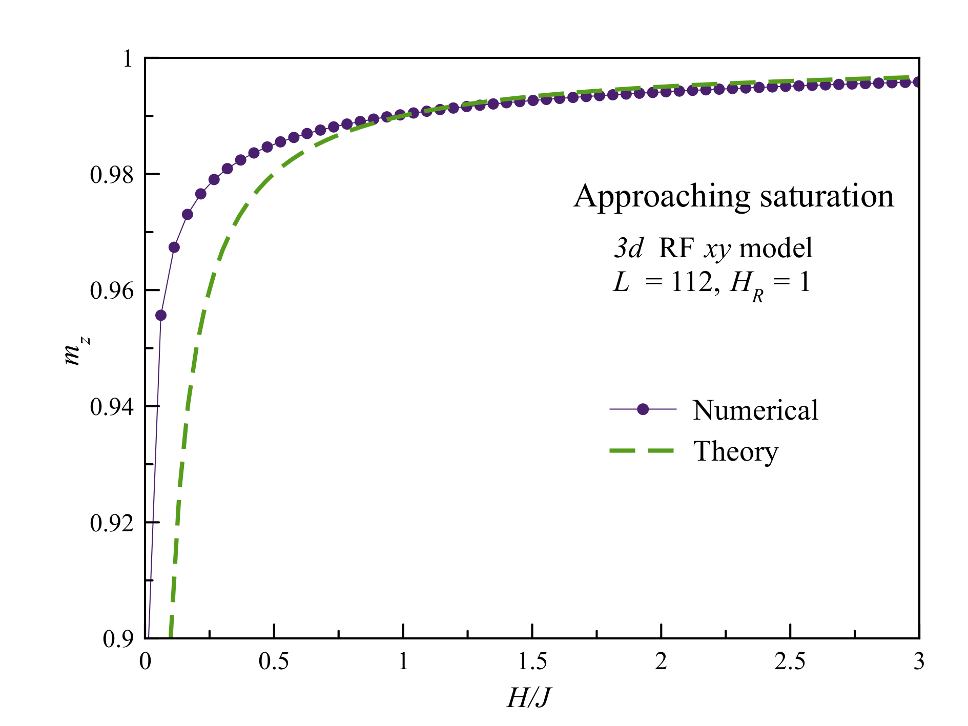
$$1-\frac{m}{s}=\langle 1-\cos\phi\rangle=\frac{1}{2}\langle\phi^{2}\rangle=\frac{1}{32\pi}\left(\frac{h}{Js}\right)^{3/2}\left(\frac{h}{H}\right)^{1/2}$$ (42)

The square root dependence on $H$, Eq. (42), must hold as long as the field satisfies $R_{H}>a$, which translates into $H<Js$. At $H>Js$ the length $R_{H}$ becomes small compared to $a$ and the exchange-generated Laplacian in Eq. (37) is no longer relevant because the $r$ in the Green function of that equation cannot be smaller than $a$. In this case the approach to saturation is dominated by the spin torque of the external field $H$ against the local field $h({\bf r})$. The Laplacian in Eq. (37) can be safely dropped and one ends up with $\phi=(h/H)\sin{\varphi}$. This gives

$$1-\frac{m}{s}=\frac{1}{2}\langle\phi^{2}\rangle=\frac{h^{2}}{2H^{2}}\langle\sin^{2}\varphi\rangle=\frac{h^{2}}{4H^{2}}.$$ (43)

Eqs. (42) and (43) are confirmed by numerical results with high accuracy, see below.

IV.5 Zero-field susceptibility

To have some reference point for comparison with numerical results, it is important to have the zero-field susceptibility of the Imry-Ma state. Application of a small field $H\rightarrow 0$ in the $x$ direction slightly perturbs $\phi({\bf r})$ created by the random field,

$$\phi({\bf r})\rightarrow\phi({\bf r})+\delta\phi({\bf r}).$$ (44)

Linearization of Eq. (36) gives

$$Jsa^{2}\nabla^{2}\delta\phi-H\sin\phi=h\delta\phi\cos(\phi-\varphi).$$ (45)

Neglecting the rapidly oscillating small term in the right-hand-side of this equation we obtain in $3d$

$$\delta\phi({\bf r})=-\frac{H}{Jsa^{2}}\int d^{3}r^{\prime}\frac{\sin({\bf r}^{\prime})}{4\pi|{\bf r}-{\bf r}^{\prime}|}.$$ (46)

The magnetization per spin in the direction of the field is given by

$$\frac{\langle m\rangle}{s} = \langle\cos\phi\rangle=-\langle\delta\phi\sin\phi\rangle$$ (47)

$$= \frac{H}{Jsa^{2}}\int d^{3}r^{\prime}\frac{\langle\sin\phi({\bf r})\sin\phi({\bf r}^{\prime})\rangle}{4\pi|{\bf r}-{\bf r}^{\prime}|}.$$

This can be related to

$$\langle{\bf s}({\bf r})\cdot{\bf s}({\bf r}^{\prime})\rangle = s^{2}\langle\cos\phi({\bf r})\cos\phi({\bf r}^{\prime})+\sin\phi({\bf r})\sin\phi({\bf r}^{\prime})\rangle$$ (48)

$$= 2s^{2}\langle\sin\phi({\bf r})\sin\phi({\bf r}^{\prime})\rangle.$$

Consequently,

$$\frac{m}{s} = \frac{H}{2Js^{3}a^{2}}\int d^{3}r^{\prime}\frac{\langle{\bf s}({\bf r})\cdot{\bf s}({\bf r}^{\prime})\rangle}{4\pi|{\bf r}-{\bf r}^{\prime}|}$$ (49)

$$= \frac{H}{2Jsa^{2}}\int d^{3}r^{\prime}\frac{\exp(|{\bf r}-{\bf r}^{\prime}|/R_{f})}{4\pi|{\bf r}-{\bf r}^{\prime}|}.$$

Integration gives

$$\frac{m}{s}=\frac{H}{2Js}\left(\frac{R_{f}}{a}\right)^{2}.$$ (50)

Zero-field susceptibility defined through

$$\frac{m}{s}=\chi\frac{H}{Js}$$ (51)

is given by

$$\chi=\frac{1}{2}\left(\frac{R_{f}}{a}\right)^{2}=128\pi^{2}\left(\frac{Js}{h}\right)^{4}.$$ (52)

In the limit of small $h$ it is very large, which may have prompted some statements in the past about infinite susceptibility of the Imry-Ma state. Aharony As we shall see below, the actual zero-field susceptibility in a zero magnetization state is dominated by the dynamics of vortices and is much smaller.

Note that the initial magnetization of the Imry-Ma state in the limit of a very weak field and the approach to saturation at a higher field can be presented as

$$\frac{m}{s}=\frac{1}{2}\left(\frac{R_{f}}{R_{H}}\right)^{2},\quad R_{H}\gg R_{f}$$ (53)

$$1-\frac{m}{s}=\frac{1}{2}\left(\frac{R_{H}}{R_{f}}\right),\quad R_{H}\ll R_{f},$$ (54)

where $R_{H}$ and $R_{f}$ are given by equations (38) and (26) respectively. Both formulas provide $m\sim s$ at $R_{H}\sim R_{f}$, which translates into

$$\frac{H}{Js}\sim\frac{1}{256\pi^{2}}\left(\frac{h}{Js}\right)^{4}.$$ (55)

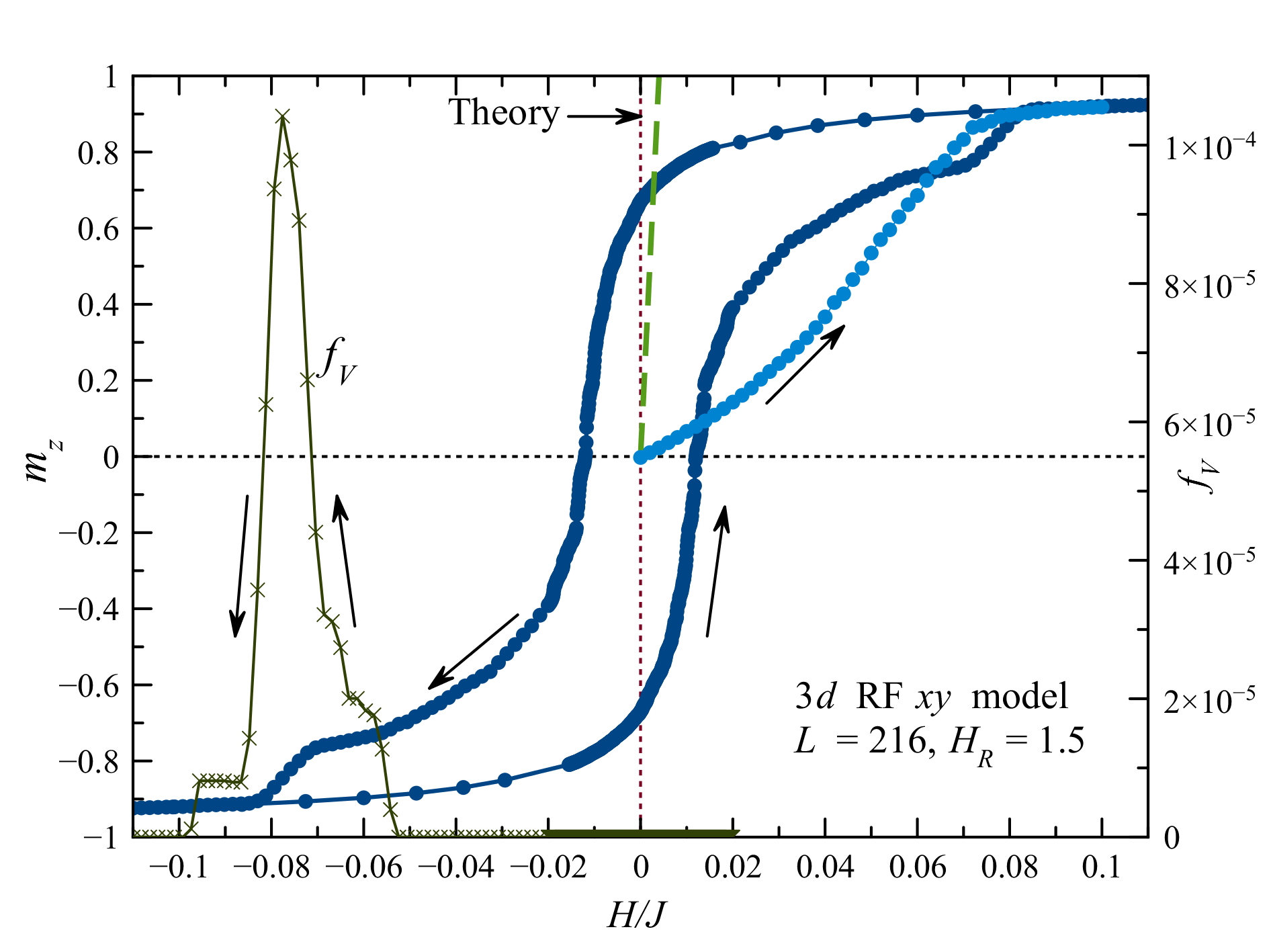
For a weak random field, $h<Js$, this gives a very small value of $H$. It has the following physical meaning. If one studies the full hysteresis loop of the random-field system then the state close to saturation must have no vortices. In this case Eq. (54) is exact. Thus, the field in Eq. (55) provides the estimate of the maximal width of the hysteresis loop. In the limit of small $h$ the loop must be very narrow, which is confirmed by our numerical results. For small $h$ one should use a very small field step in order not to confuse a very steep magnetization curve with a discontinuity in the magnetization curve. When the width of the hysteresis loop is so small that it cannot be resolved in either real or numerical experiment, its slope may well be described by Eq. (52).

IV.6 Average magnetization of a finite system

As we have seen, at $h<Js$, the regions that are ferromagnetically ordered can be quite large. A system of size $L<R_{f}$ will always exhibit ferromagnetic order. Thus, it may be difficult to numerically test the Imry-Ma statement that a random field, however weak it may be, destroys the long-range order in three dimensions. Even when $R_{f}$ is small compared to $L$ it may not be easy to distinguish between spontaneously magnetized states and zero-magnetization states because of the magnetization arising from statistical fluctuations. The problem is similar to that of a finite-size paramagnet: $N$ spins randomly distributed between spin-up and spin-down states will have an average total magnetization proportional to $\sqrt{N}$ and thus average magnetization per spin proportional to $1/\sqrt{N}$.

The magnetization of the system is given by

$$\mathbf{m}=\frac{1}{N}\sum_{i}\mathbf{s}_{i},$$ (56)

where $N$ is the total number of spins. The absolute value of $m$ is related to the spin correlation function of Eq. (10) as

$$m^{2}=C(\infty)+\frac{1}{V}\int d^{d}R\left[C(\mathbf{R})-C(\infty)\right],$$ (57)

where $C(\infty)$ describes long-range order (LRO) and $V=L^{3}$ is the system volume. Plotting $m^{2}$ vs $1/V$ shows if there is a LRO in the system in the limit $V\rightarrow\infty$.

Substituting here $C(\mathbf{R})=s^{2}\exp(-R/R_{f})$ (no long-range order) in $3d$, one obtains

$$m=s\left(\frac{8\pi R_{f}^{3}}{V}\right)^{1/2}=\sqrt{8\pi}s\left(\frac{R_{f}}{L}\right)^{3/2},$$ (58)

where $L$ is the size of the system, $N=(L/a)^{3}$. At, e.g., $h=0.5Js$, the Imry-Ma correlation length is $R_{f}\approx 200a$. For $L=1000a$ this gives $m\approx 0.45s$. Such a large value of $m$ for a not very weak random field in a system of the maximum size that we can access numerically suggests that any evidence of the long-range ferromagnetic order based upon finite $m$ should be dealt with care. However, LRO, if it is present, reduces the value of the $1/V$ term in Eq. (57).

IV.7 Correlated random field

All the above formulas have been written for uncorrelated random field described by Eq. (4). Meanwhile, in physical problems involving flux lattices and random magnets, the static randomness can be correlated over a certain distance $\rho>a$. Such situation is described by Eq. (5). It is easy to see that it leads to the following modification of $R_{f}$ in Eq. (23):

$$\frac{R_{f}}{a}=\frac{16\pi a^{3}}{\Omega}\left(\frac{Js}{h}\right)^{2},$$ (59)

where

$$\Omega=\int d^{3}r\Gamma(r)$$ (60)

is the correlated volume, with $\Gamma(r)$ describing the short-range correlations of the random field.

For uncorrelated random field one has $\Omega=a^{3}$ and Eq. (59) goes back to Eq. (26). In the case of a correlated random field $\Omega>a^{3}$ and $R_{f}$ is reduced. For, e.g., $\Gamma=\exp(-r/\rho)$, one obtains $\Omega=8\pi\rho^{3}$ and

$$\frac{R_{f}}{a}=2\left(\frac{a}{\rho}\right)^{3}\left(\frac{Js}{h}\right)^{2}.$$ (61)

Notice that the reduction in $R_{f}$ is by a factor $8\pi(\rho/a)^{3}$ which can be quite significant. This, in principle, may allow one to test the effect of a very small $h$ in a finite-size system. When the above formulas produce $R_{f}<\rho$, this means that $R_{f}=\rho$.

V Numerical results

V.1 Numerical method

Figure 1: Efficiency of the weak-damping (slow-cooling) method for glassy systems.

The task is to find energy minima of Eq. (1) by a numerical algorithm starting from an initial state (IC) and using some relaxation protocol. It turns out that there are multitudes of local energy minima and the situation resembles that of a spin glass. At the end of relaxation the system ends up in one of them. We do not attempt to search for the ground state of the system, which would require different numerical methods. Rather, we are interested in representative local minima obtained by relaxation from typical IC such as random and collinear initial conditions. This corresponds to experimental situations, and the results for physical quantities in the final state are reproducible up to statistical noise due to different realizations of the random field and different realizations of the relaxation protocol that may have a stochastic part. The larger the system size, the smaller the fluctuations. For smaller sizes, averaging of the results over realizations of the random field is necessary.

One could use the Landau-Lifshitz equation of motion with damping (with no precession term for the $xy$ model) to find local energy minima. One can expect an even faster relaxation if one rotates every spin, sequentially, straight in the direction of the effective magnetic field

$$\mathbf{H}_{i,\mathrm{eff}}=\sum_{j}J_{ij}\mathbf{s}_{j}+\mathbf{h}_{j}+\mathbf{H}$$ (62)

that is Dieny-PRB1990

$$\mathbf{s}_{i,\mathrm{new}}=\mathbf{H}_{i,\mathrm{eff}}/\left|\mathbf{H}_{i,\mathrm{eff}}.\right|$$ (63)

We call this the finite rotation (FR) method. Although this method works very well in cases when there is only one energy minimum (such as the collinear state for pure ferromagnetic models), it leads to slow relaxation in the case of glassy behavior characterized by many local minima. The problem is that the relaxation described by Eq. (63) is initially too fast and the system falls into the nearest local minimum that is not the deepest and not the most representative. As in the multi-dimensional space of our model there are narrow valleys rather than simple local minima, the system quickly falls into one of these valleys and then begins a long travel along it.

To counter this slow relaxation, it is convenient to combine the FR method with so-called over-relaxation Adler-PRD1981 that is, in fact, a conservative pseudo-dynamics described by

$$\mathbf{s}_{i,\mathrm{new}}=\frac{2\left(\mathbf{s}_{i,\mathrm{old}}\cdot\mathbf{H}_{i,\mathrm{eff}}\right)\mathbf{H}_{i,\mathrm{eff}}}{H_{i,\mathrm{eff}}^{2}}-\mathbf{s}_{i,\mathrm{old}}.$$ (64)

Here spins are sequentially flipped onto the other side of the effective field (half of the precession period for the Heisenberg model) and the energy is conserved. This method is very convenient to quickly explore the hypersurface of constant energy of the system. Whereas the FR method searches for a minimal energy, the over-relaxation method searches for the maximal entropy. It is a standard numerical method for classical spin systems, usually combined with Monte Carlo updates (see, e.g., Ref. Chen-Landau-PRB1994, ).

For instance, starting from the collinear state and using the over-relaxation method, one can describe FR-induced transition of the system from the initial state that has the minimal statistical weight to a more disordered state having the same energy but a much higher statistical weight. This process describes an irreversible relaxation in which the magnetization value $m$ decreases from 1 to a smaller value. The resulting final state is above the ground state, so it can be interpreted as a thermal state with some small temperature. Adding the energy-lowering evolution described by Eq. (63) one can find the lowest-energy state in this particular region of phase space.

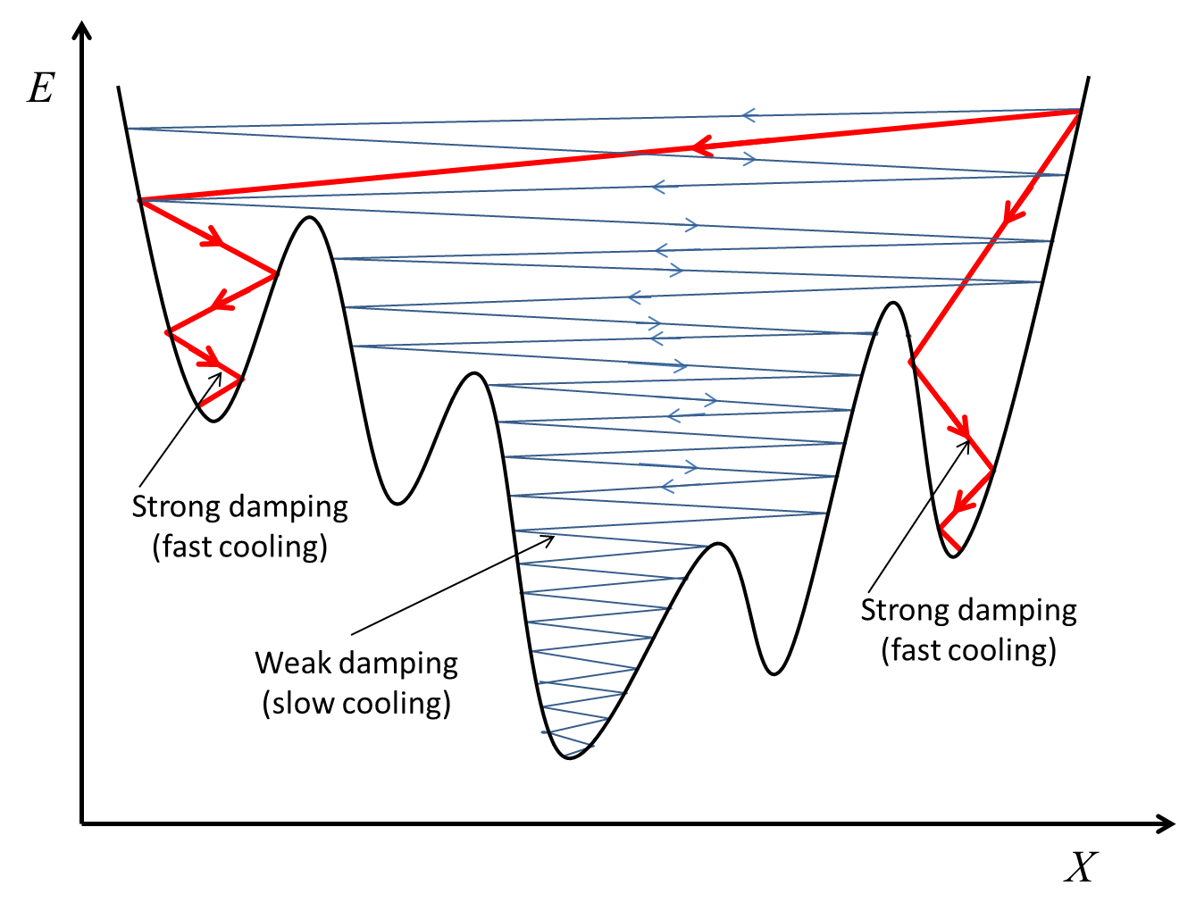
Practically it is convenient to combine both methods. In the main method we used, Eq. (63) is applied with the probability $\alpha$ while Eq. (64) is applied with the probability $1-\alpha$. The optimal value of $\alpha$ that plays the role of a relaxation constant is in the range $0.1-0.01,$ typically 0.03. Physically this corresponds to slow cooling the system. Such a choice results in convergence acceleration by factors greater than 10 in comparison to $\alpha=1$. The efficiency of the combined weak damping method for glassy systems is shown in Fig. 1, assuming that deeper minima have broader basins of attraction.

Starting from the collinear state, we also used a two-stage relaxation method. The first stage, which we call “chaotization”, is the conservative pseudo-dynamics given by Eq. (64). The second stage is the combined relaxation process described above. In some cases during chaotization damped oscillating behavior was observed. In this case suppression of oscillations and a faster convergence can be achieved by performing Eq. (64) with a probability $1-\eta$ and leaving the spin unchanged with the probability $\eta$. The constant $\eta$ that has the optimal value about 0.01 plays the role of a decoherence constant in the numerical method.

To check the predicted absence of ordering in RF magnets, one has to numerically solve models of a size $L\gg R_{f}$ that must be strongly fulfilled in accordance with the discussion in Section IV.6. This sets a lower bound on the numerically accessible $H_{R}\equiv h$. With a Mac Pro with 96 GB RAM running Wolfram Mathematica, we can compute $3d$ models up to the size $L=800$, i.e., half a billion spins, including correlation functions. The memory usage during relaxation to the energy minima is about 30 GB while computation of the correlation function takes 85 GB. This means that we cannot further increase the size while computing correlation functions, although we can compute the relaxation of a system of $L=1000,$ a billion spins. Our Mathematica program that uses compilation and parallelization is comparable in speed with programs written in Fortran and C. Relaxation of a $3d$ system of $L=800$ for moderately small $H_{R}$ takes 1-2 days.

We also compute the vorticity by analyzing rotation of spin vectors along any unitary square plaquette in $xy$ planes. If spins rotate by 0 angle along the plaquette, there is no singularity of the spin field at this plaquette. If spins rotate by $\pm 2\pi$, there is a vortex or antivortex. For initial states that have no global vorticity, such as collinear and random initial state, the numbers of vortices and antivortices are always the same. Thus we just count them as “vortices” and define vorticity $f_{V}$ as the fraction of plaquettes that contain singularities. In the random state one has $f_{V}=1/3$ while in the energy minima that we find $f_{V}$ is zero or a small number. In the latter case there are vortex loops in the system.

In the numerical work we use $J=a=s=1$.

Our lowest value of $H_{R}$ in $3d$ is 0.7, which corresponds to $R_{f}=103$ and is still much smaller than our largest size, $L=800$, and convergence of our method is still fast enough. For $H_{R}=0.5$ one has $R_{f}=201$, so that that the ratio $R_{f}/L$ is not small enough even for $L=800$ and here convergence of our method is noticeably slower. Although we can reach an energy minimum in this case spending more time, the resulting correlation functions depend on the realization of the random field and are bumpy. This is the consequence of insufficient self-averaging for $R_{f}/L$ not small enough. In this case additional averaging over random-field realizations is needed, which for $L=800$ would take too much time. To the contrary, if $R_{f}/L\ll 1$ is strongly satisfied, self-averaging is sufficient and correlation functions have a smooth shape. Also in this case convergence of our method is pretty fast. For instance, relaxation of the system of $L=800$ out of a collinear state takes only about 5 hours. For smaller sizes we do averaging over realization of the random field to achieve a better precision.

Computations in $2d$ are numerically less challenging, in particular, because of the much shorter $R_{f}$. Finding a local minimum of the energy at $T=0$ for $L=10000$ (100 millions of spins) and $H_{R}=0.1$ does not present problems.

V.2 General results

Our main finding is that for a weak random field the state of the system is always a glassy state with many local energy minima, so that the final state that we find depends on the initial state or initial condition, as well as somewhat on the details of the relaxation protocol. This to a some degree disqualifies earlier attempts to describe the random-field system by a unique magnetic state. Instead, the system exhibits magnetic hysteresis similar to that in conventional ferromagnets with pinning of the domain walls.

Starting from random initial condition we find states having small values of $m$ (decreasing to zero in the large-size limit) and substantial vorticity. For $R_{f}\gg 1$ there is a strong short-range order everywhere except the vicinity of vortex loops. The correlation function in this state decays to zero but the correlation length is defined by the average distance between the vortices rather then by $R_{f}$, the former being much shorter. We call this state a vortex glass (VG).

Figure 2: Magnetization relaxation curves starting from a collinear initial condition. The method with a small damping constant, $\alpha=0.01-0.03$ is most efficient.

Figure 3: Two-stage relaxation starting from a collinear state for $H_{R}=1.5$ and $L=800$ and one-stage relaxation for $H_{R}=0.5$ and $L=1000$, our largest system size. Note a slow relaxation for $H_{R}=0.5$.

Starting from the collinear initial condition, for $H_{R}\lesssim 2$ we find only partially disordered states having $m$ still of order 1 (stable in the large-size limit) and zero or extremely small vorticity. In this state, the correlation function follows Eq. (26) at short distances but reaches a plateau at longer distances, thus showing a long-range order. We call this state ferromagnetic, although it should be stressed that the system does not order spontaneously on lowering temperature but freezes into the vortex glass state instead.

For $H_{R}\gtrsim 2,$ starting from the collinear initial state, vortex loops are spontaneously generated and magnetization is strongly reduced.

The energy of the VG state is always higher than the energy of the ferromagnetic state. (This holds for both $xy$ and Heisenberg models in $1d$, $2d$, and $3d$, as well as for random-anisotropy models.) Thus the vortex glass state is a metastable state that could, in principle, relax to the ferromagnetic state by eliminating vortex loops that cost energy. However, this does not happen because vortex loops are pinned by the random field. It is possible that the ferromagnetic state is also a metastable state, while there is a true ground state with $m=0$, in accordance with the implicit theorem by Aizenman and Wehr. Aizenman-Wehr-PRL ; Aizenman-Wehr-CMP However, we were unable to find this state by relaxation from typical states. To the contrary, sampling local energy minima shows that starting with a low $m$ state it is easier to find lower energy states with higher $m$ than with lower $m$.

V.3 Relaxation from the collinear state leading to a ferromagnetic state

Figure 4: Relaxation starting from differently oriented collinear states for the same realization of the random field, showing glassy nature of the RF magnet.

Figure 5: Relaxation from collinear states for different realization of the random field. Statistical scatter decreases with the system size due to self-averaging. a) $L=128$; b) $L=256$.

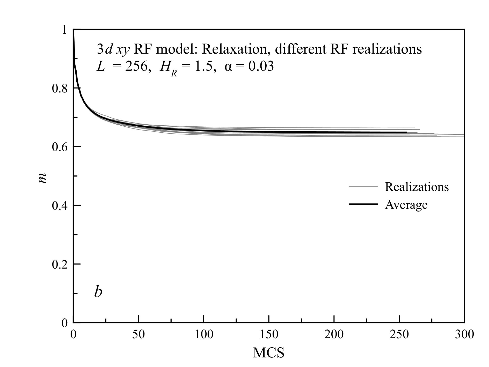
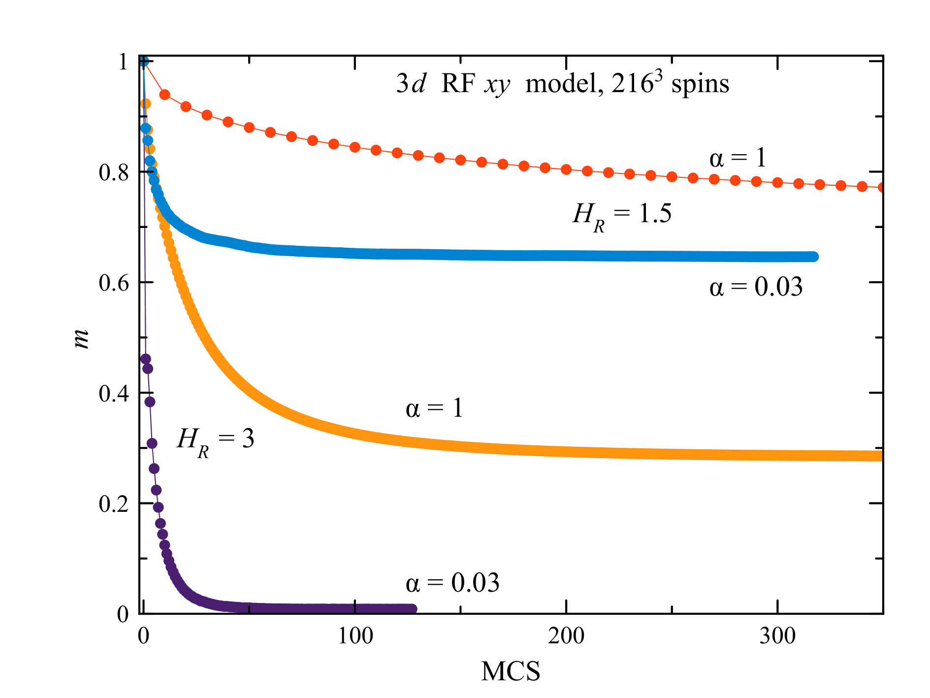
During relaxation from any of the initial states we have tried, the system’s energy decreases. Starting from the collinear initial condition, $m$ decreases until it reaches a constant value for $H_{R}\lesssim 2$ and goes to zero at $H_{R}\gtrsim 2$. Direction of the magnetization vector $\mathbf{m}$ practically does not deviate from the initial direction. Fig. 2 shows relaxation curves for $H_{R}=1.5$ with $m$ approaching a nonzero constant and for $H_{R}=3$ with $m$ going to zero. One MCS (Monte Carlo Step) means one complete spin update of the system. We use this standard notation although we are not using Monte Carlo. One can see that the pure finite rotation method ($\alpha=1$) is slow for our problem in comparison to the combined method predominantly using over-relaxation ($\alpha=0.03$). For $H_{R}=3$, the system gets stuck in a metastable state with $m\approx 0.3$ and $\Delta E=-0.668$. However, the combined method finds the state with a very small $m$ and the lower energy $\Delta E=-0.671$. Here $\Delta E\equiv E-E_{0}$, where $E_{0}$is the exchange energy of the collinear state, $-3J$ for the $3d$ model with periodic boundary conditions (pbc). These results are in accordance with the mechanism of relaxation sketched in Fig. 1.

In fact, already the pure over-relaxation method ($\alpha=0$) provides a fast relaxation of $m$ at a constant energy. For this reason in some computations we used the two-stage method, as shown in Fig. 3. The idea is that the conservative over-relaxation method has a potential for the maximal possible disordering since it leads to states that can be interpreted as thermal states with a small $T$ (the over-relaxation plateau in Fig. 3). As the energy-relaxation mechanism is switched on, this temperature goes to zero and ordering in the system increases, as is seen in the Fig. 3. The states obtained in these computations are vortex free.

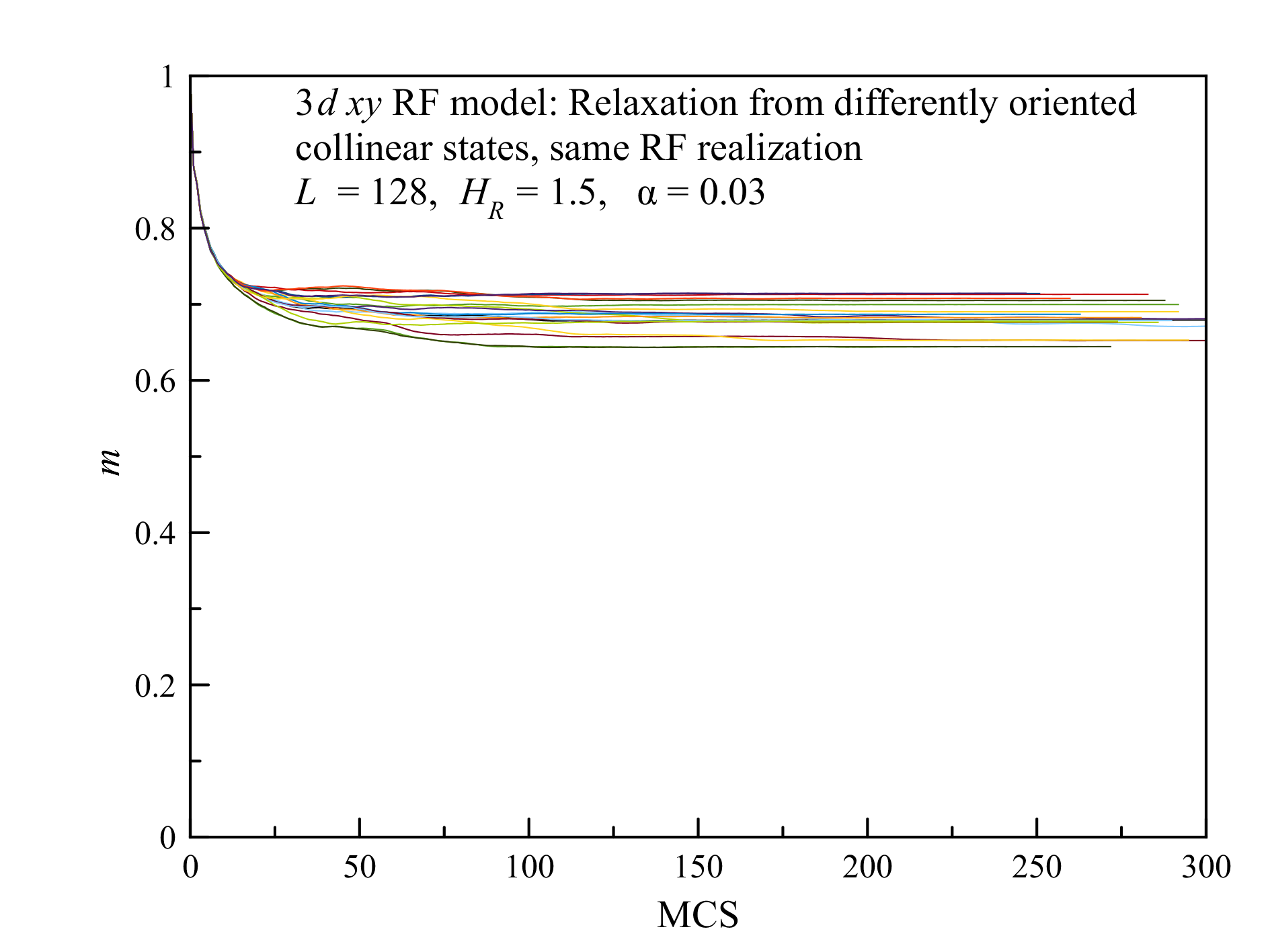
Fig. 4 obtained by multiple relaxation events of a system with the same realization of the RF from differently oriented collinear states shows different local energy minima achieved in different cases. This confirms glassy nature of a random-field magnet. All these states are vortex-free, as above.

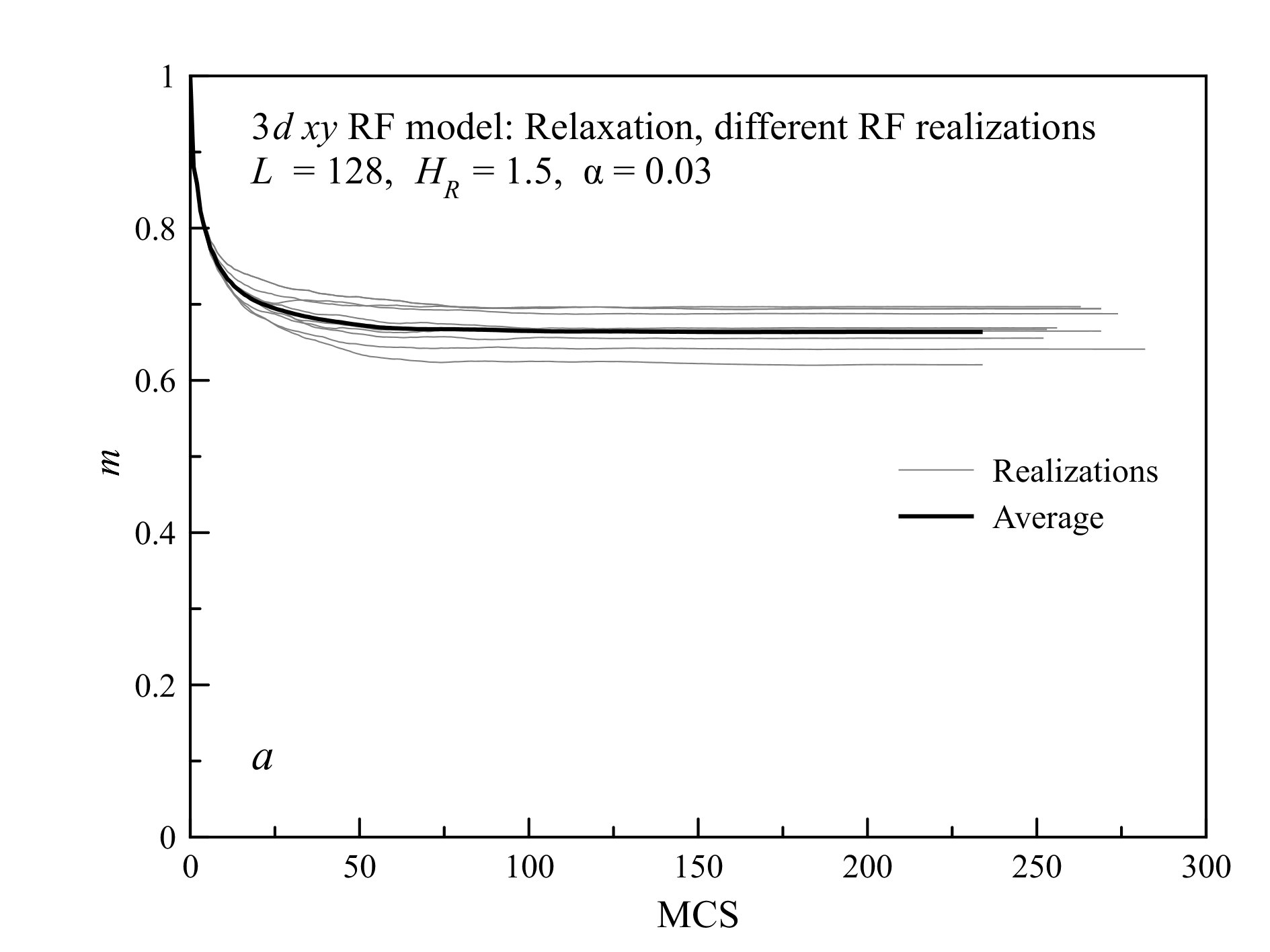
Fig. 5 shows similar computations with different realization of the RF. One can see that Fig. 5$a$ is similar to Fig. 4. Comparison of the two panels of Fig. 5 shows that the statistical scatter decreases with the system size because of self-averaging. For the standard deviation $\Delta m$ of the magnetization in the final state one has $\Delta m\approx 0.025$ for $L=128$ and $\Delta m\approx 0.0097$ for $L=256$. On the other hand, $\Delta mL^{3/2}\approx 36$ for $L=128$ and $\Delta mL^{3/2}\approx 39$ for $L=256$ that are nearly the same. This is in accord with the picture of correlated regions of linear size $R_{f}$ that are oriented independently from each other, leading to

$$\Delta m\propto\left(\frac{R_{f}}{L}\right)^{3/2}.$$ (65)

Using $R_{f}$ of Eq. (23) and the numerical factor from the computational results above, one can estimate the statistical scatter in all other cases.

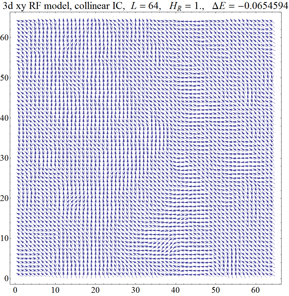
The structure of the ferromagnetic state shown in Fig. 6 has no singularities.

Figure 6: Spin configuration obtained for $H_{R}=1$ from the collinear initial condition

Figure 7: Magnetization squared in the ferromagnetic state vs system volume $V=N$. Italicized numbers are those of RF realizations used to compute the averages of $m$. Upright numbers below points indicate the systems’ linear size $L$. Straight dashed lines are guides for the eye.

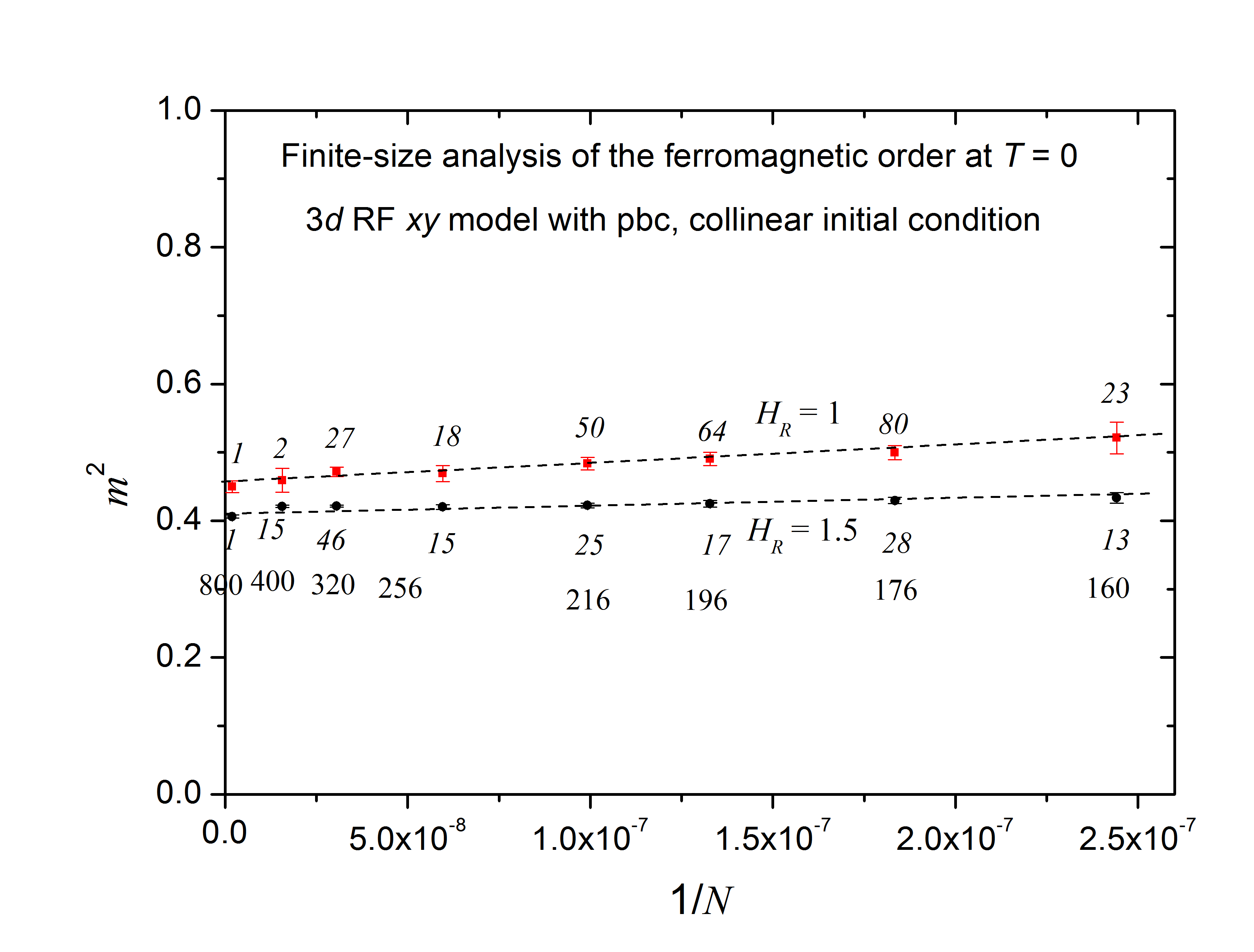
With increasing the system size the numerically found $m$ does not decrease to zero, as one can see by comparing Figs. 2 and 3. The stability of the ferromagnetic state is clearly seen from the finite-size analysis shown in Fig. 7. Here all points except for $L=800$ have been obtained by averaging over realizations of the random field, the number of realizations indicated by the italicized numbers. Although there is self-averaging in the system, averaging over realizations allows to further reduce data scatter. One can see that the points fall on straight lines with a finite offset, in accordance with Eq. (57). The error bars are the uncertainties of the average values computed as $\Delta m/\sqrt{n}$, where $\Delta m$ is the standard deviation defined by Eq. (65) and $n$ is the number of realizations.

V.4 Relaxation from the wavy state

Figure 8: Wavy state of spins in the $xy$ plane

Figure 9: Magnetization relaxation from the collinear and wavy initial states.

Figure 10: Local energy minima, labelled by the corresponding magnetization values, obtained by evolution from wavy states, Eq. (66), with $k_{x,y,z}=0,1,2,3$.

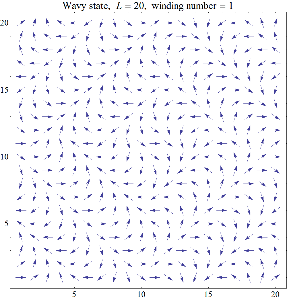
One can argue that the ferromagnetic state obtained from the collinear initial state is an artefact and ferromagnetism here is preselected. An argument in support of ferromagnetic state can be obtained by starting from a special kind of initial state that has $m=0$ and no vortices or helicity. In this state, which we call a wavy state, spins rotate in one direction and then in the opposite direction when the observer is moving in any of the three directions in the cubic lattice. It is defined by

$$\left(s_{x},s_{y}\right)=\left(\cos\left(\Phi\right),\sin\left(\Phi\right)\right),$$ (66)

where

$$\Phi=\frac{2\pi k_{x}n_{x}}{N_{x}}\left(-1\right)^{\left[k_{x}n_{x}/N_{x}\right]}+(x\Rightarrow y)+\left(x\Rightarrow z\right).$$ (67)

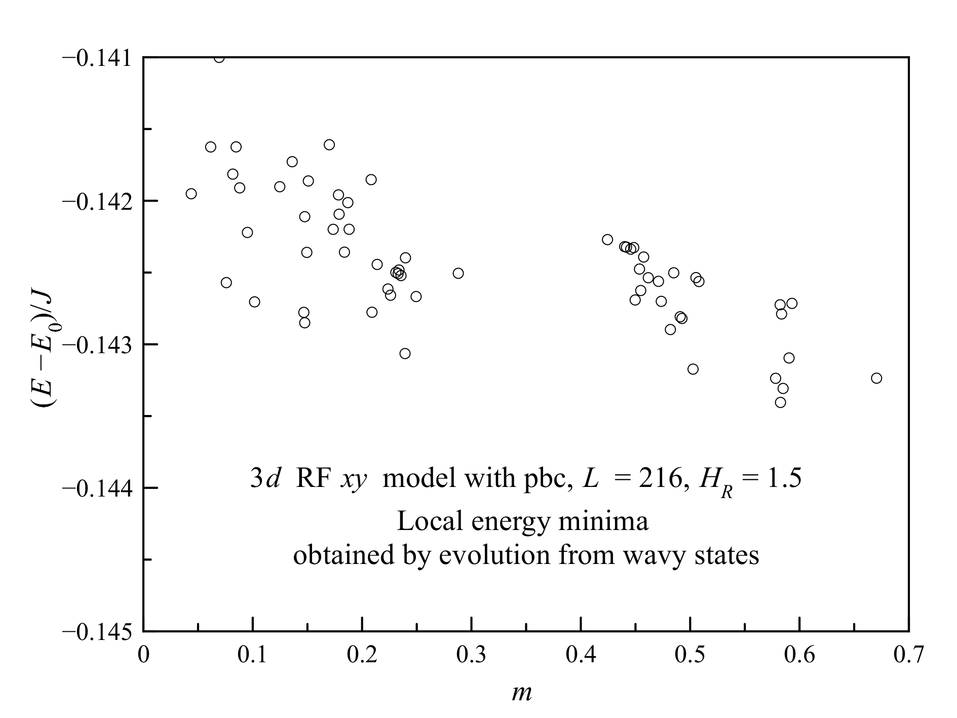
Here $N_{x,y,z}$ are lattice sizes, $n_{x,y,z}=1,\ldots,N_{x,y,z}$ are lattice positions, $k_{x,y,z}$ are corresponding wave vectors and $\left[x\right]$ means integer part. The wavy state is topologically equivalent to the collinear state because it can be transformed into the latter by continuous deformations without changing the topology. This state resembles a spring that tends to straighten when released. Its energy is $\sim J(a/L)^{2}$ above that of the collinear state. An example of a wavy state is shown in Fig. 8. Fig. 9 shows magnetization relaxation curves starting from the collinear and wavy initial conditions that lead to the same final state with a high $m$. It must be noted that restoration of a large $m$ out of the wavy state does not always take place. For $H_{R}\gtrsim 2$ vortices are generated spontaneously out of any vortex-free state, including the wavy state, so that the final state is a vortex glass with $m$ close to zero. Even for $H_{R}=1.5$ the system randomly lands in (vortex-free) states with small and large $m$, see Fig. 10. Note that states with higher $m$ in Fig. 10 typically have a lower energy.

V.5 Vortex-glass state

Figure 11: Spin configuration obtained for $H_{R}=1$ from a random initial conditions. Vortices/antivortices are shown by blue/red circles.

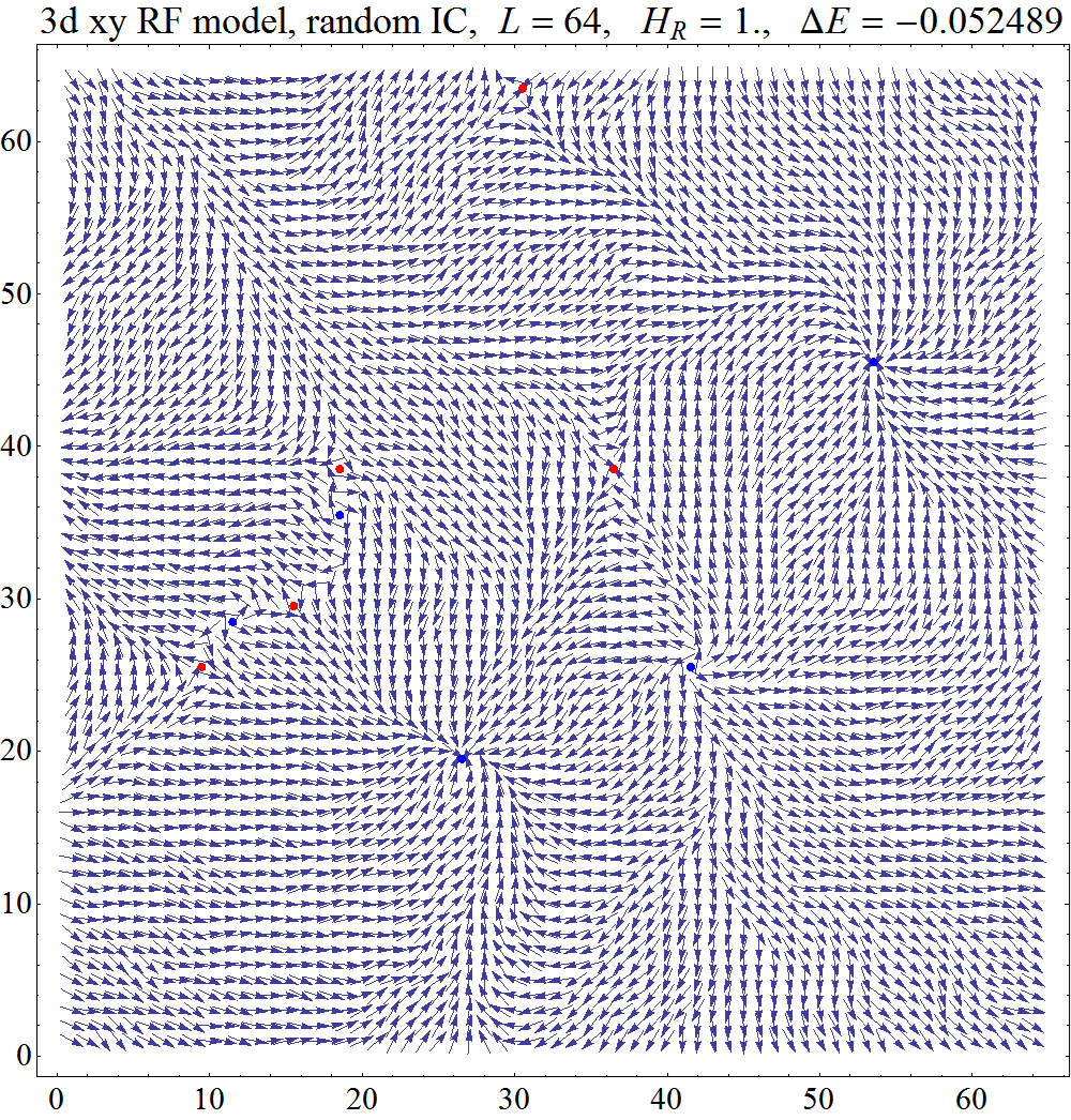
The vortex-glass state contain singularities, vortices and antivortices, shown in Fig. 11. In our $3d$ case these are vortex lines going through the sample and vortex loops.

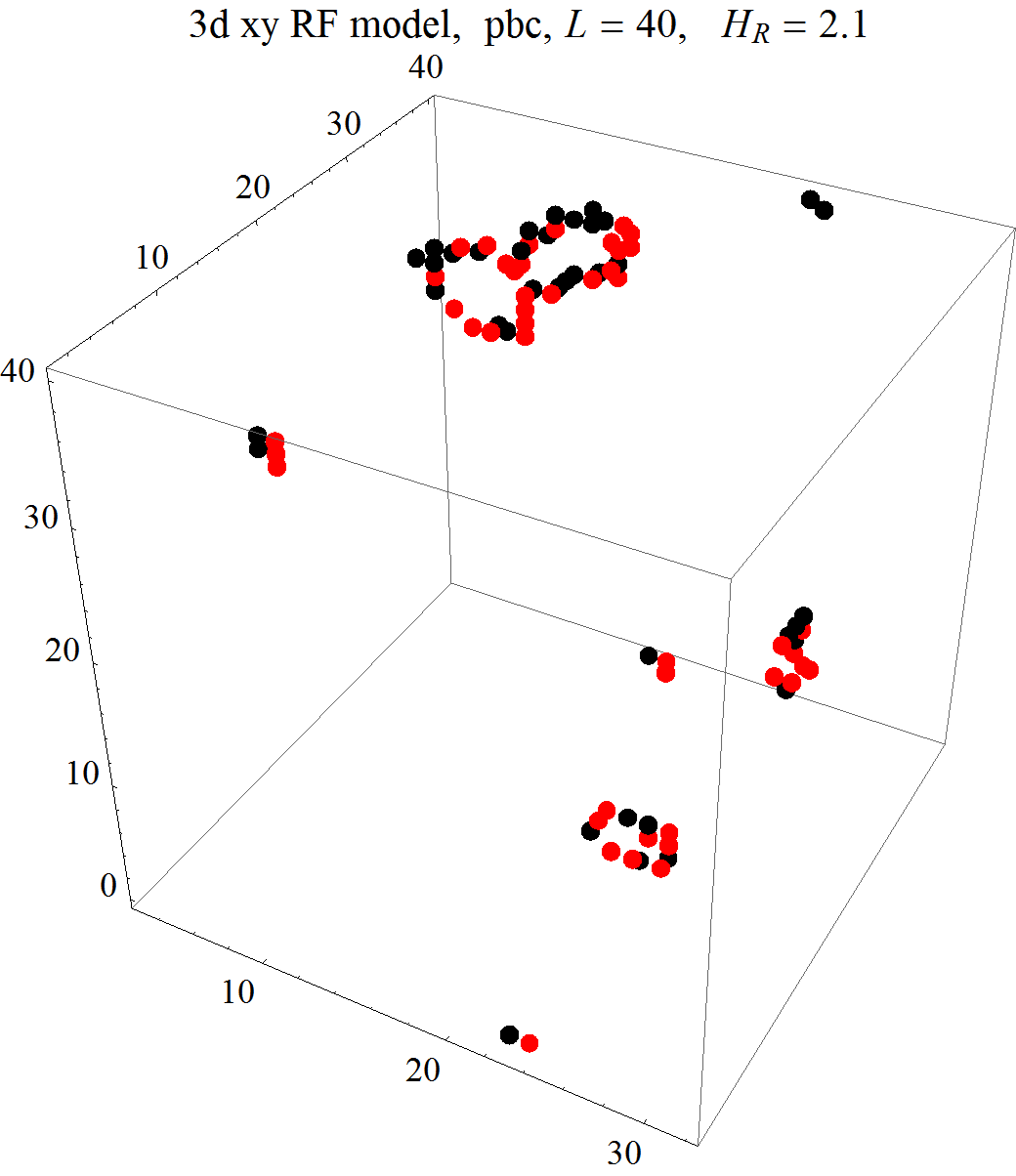
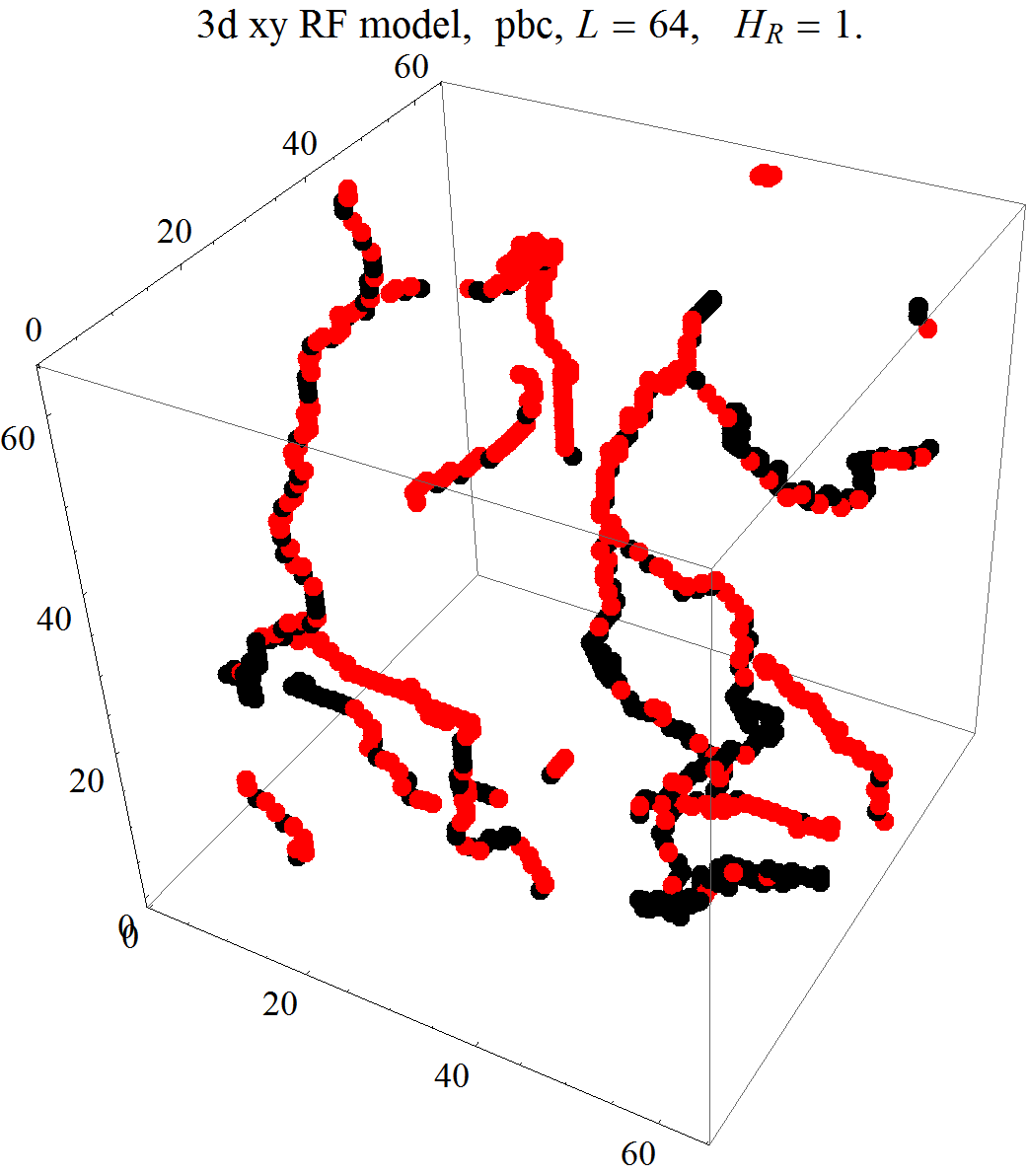
For larger $H_{R}$ vortex loops are created by the random field even starting from the collinear initial condition. For any system size, there is a critical value $H_{R,c}\approx 2$ above which vortex loops emerge. Slightly above $H_{R,c}$ these vortex loops are short, as shown in Fig. 12 (top). With increasing $H_{R}$, vortices quickly proliferate into the system and the number and length of vortex loops increase. It is difficult to prove whether there exists a size-independent threshold value $H_{R,c}$. Computations show that $H_{R,c}$ slowly decreases with the size. However, this question seems to be not very important because the vorticity increases with a very small slope above the threshold. It may be that in the bulk there are vortex loops at any finite $H_{R}$ but the vorticity for small $H_{R}$ is extremely low.

Meanwhile, starting from random initial conditions one arrives at states with long vortex lines that typically do not close into loops but cross the system’s boundaries, see Fig. 12(bottom). As vortices and antivortices can exist in all three available planes, different singularities may exist at nearly the same point, e.g., a vortex in the $xy$ plane may occupy the same point as an antivortex in the $yz$ plane. For this reason, some points in the figure may contain both black and red paints.

Obtaining VG states with our algorithm amounts to slow cooling the system. We have checked with Monte Carlo simulations that slow lowering the temperature leads to the same effect: the system does not order ferromagnetically but rather freezes into the VG state that for $H_{R}<H_{R,c}$ has a higher energy than the ferromagnetic state.

Figure 12: Vortex loops in $3d$ xy RF model. Collinear (top) and random (bottom) initial conditions. Vortices/antivortices are shown by black/red.

V.6 Magnetization and vorticity

Figure 13: Magnetization vs the random field strength $H_{R}$ for the model with pbc of the size $L=216$.

Figure 14: Finite-size analysis of the magnetization in the vortex-glass phase

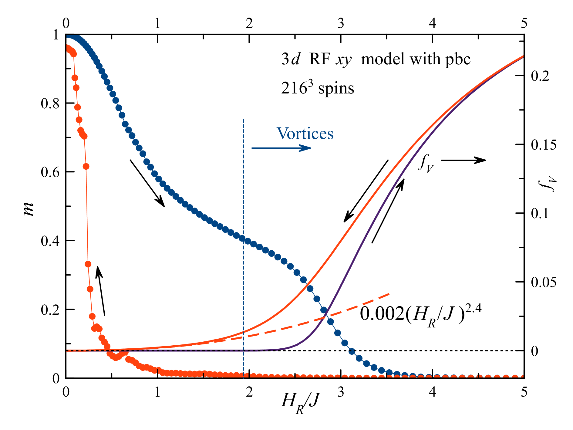
The magnetization $m$ and vorticity $f_{V}$ as functions of $H_{R}$ are shown in Fig. 13. Here the same realization of the random field was used and only its strength $H_{R}$ was changed in small steps, using final states for a given $H_{R}$ as initial conditions for the next value of $H_{R}$. Different random-field realizations result in slightly different curves.

At $H_{R}=5$ vorticity is very high and it decreases upon lowering $H_{R}$. The magnetization remains very small as the system enters the vortex glass phase with a small but nonzero $f_{V}$. For $L=216$ the number of vortex lines in the system becomes small below $H_{R}=1$ [see Fig. 12(bottom)] and $m$ starts to increase. For larger $L$, this happens at smaller $H_{R}.$ In some cases the system reaches a collinear state with $m=1$ at $H_{R}=0$. In other cases, as in Fig. 13, the system ends up in a topologically stable state with nonzero helicity (for pbc) and $m<1$.

The magnetization in the ferromagnetic state decreases with $H_{R}$ as shown in Fig. 13, starting from the pure limit $m=1$ at $H_{R}=0$. For $H_{R}<1.8$ this state is vortex-free. Proliferation of vortices for $H_{R}>1.8$ results in the shoulder of this curve and full destruction of the order at $H_{R}>4$.

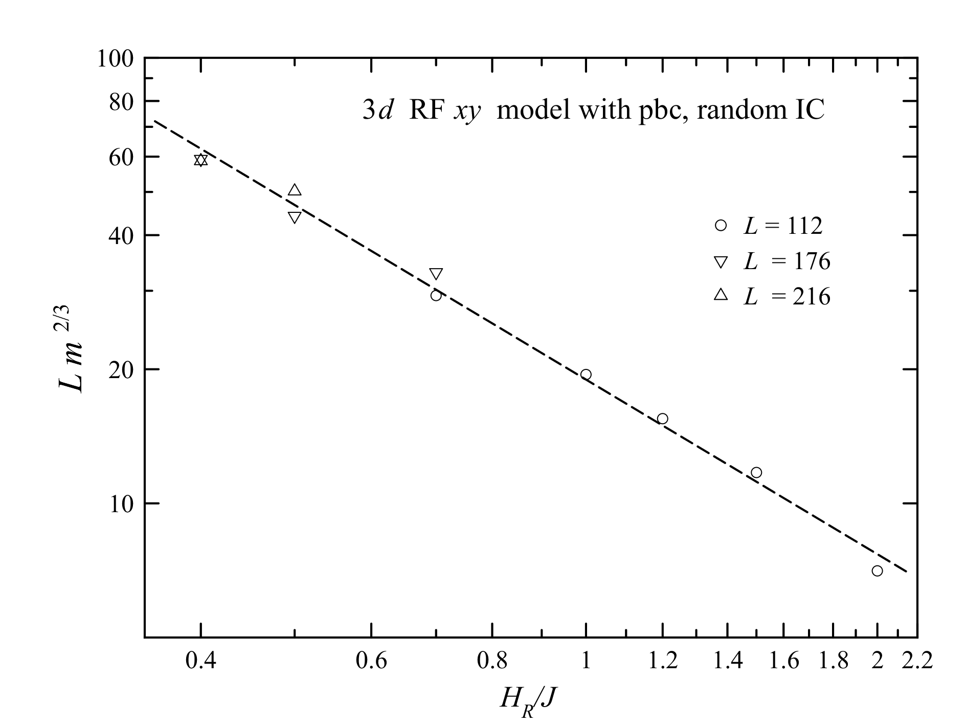
The magnetization of the VG state for $H_{R}<H_{R,c}$ is small and it scales as $m\propto 1/L^{3/2}$, in accordance with Eq. (58), as shown in Fig. 14. Putting together data obtained for different $L$ and $H_{R}$ data, averaged over many RF realizations, one obtains the dependence of the correlation radius of the VG phase $R_{V}$ that replaces $R_{f}$ of Eq. (23). The result is

$$R_{V}\propto 1/H_{R}^{1.2}$$ (68)

that is much shorter than $R_{f}$ at small $H_{R}$. The numerical factor in this formula cannot be found by this method because the form of the CF in the VG state is different from the simple exponential. The precise form of $R_{V}$ will be found in the section on correlation functions below.

On the other hand, vorticity data in the VG state in Fig. 13 can be roughly fitted to the form

$$f_{V}\approx 0.002(H_{R}/J)^{2.4}.$$ (69)

Combining the two formulas above yields

$$R_{V}\propto 1/f_{V}^{1/2}.$$ (70)

It is clear that vortices are the main reason for the decay of spin-spin correlations in the vortex glass for $R_{V}\ll R_{f}$ . Thus there must be a relation between $R_{V}$ and the vorticity $f_{V}$ defined as the fraction of unit plaquettes with vortices or antivortices. Naively one could expect that $R_{V}$ is proportional to the distance between the singularities, so that in $3d$ one has $R_{V}\propto 1/f_{V}^{1/3}$. As vortex lines are linear objects, $R_{V}$ is proportional to the average distance between vortex lines. This makes the situation effectively two dimensional.

V.7 Energy

Figure 15: Energy vs the random field strength $H_{R}$ in the ferromagnetic and vortex-glass states. The dashed green line labelled “theory” is Eq. (35). Inset: Fitting the energy in the vortex-glass state.

Figure 16: Energies of metastable vortex-glass states sampled vs their magnetization. Energy values in the vortex-glass state show a perfect correlation with their vorticities. Energies of vortex-free ferromagnetic states are comparable to those in Fig. 23.

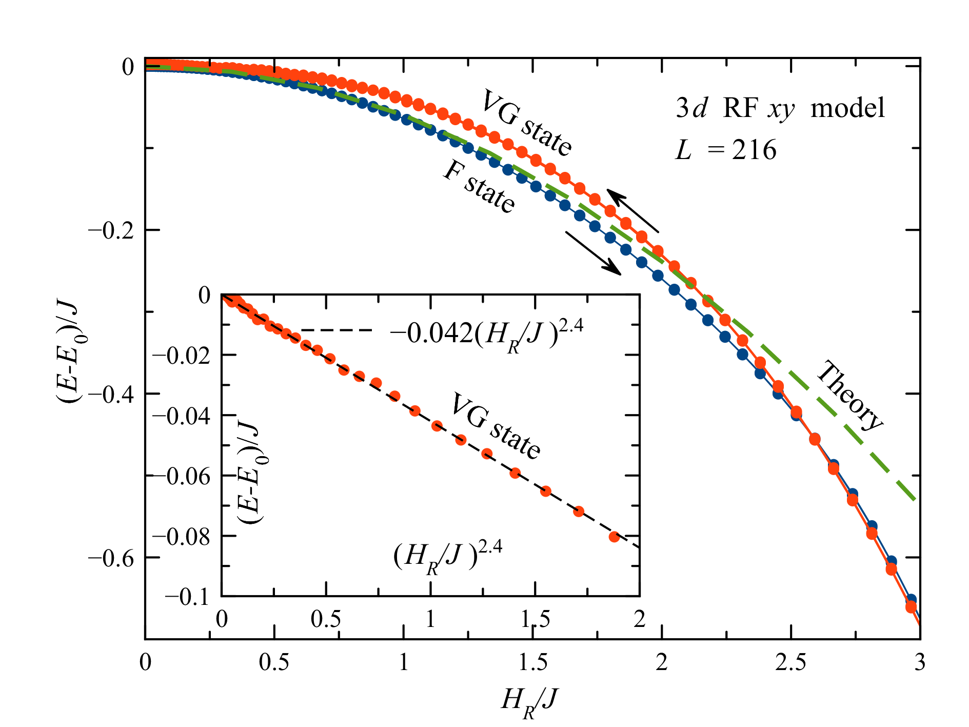
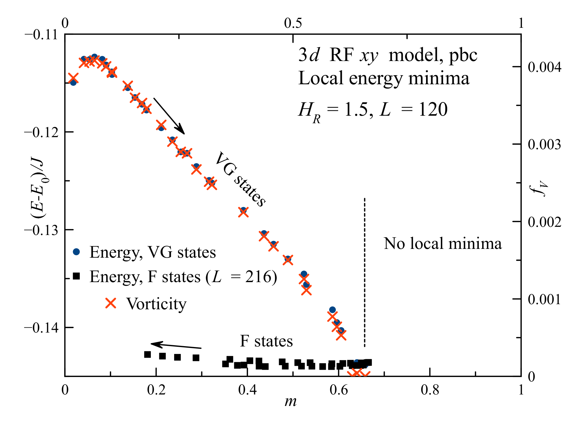
Fig. 15 obtained from the same computation as Fig. 13 shows that the energy of the vortex-glass state is higher than the energy of the ferromagnetic state everywhere except for $H_{R}>2.5$ where creation of vortices becomes energetically favorable. However, at these large values of $H_{R}$ the destruction of the ferromagnetic state begins, see Fig. 13. Thus the vortex-glass state is metastable in the most interesting region of small $H_{R}$. The energy of the ferromagnetic state follows Eq. (35) in the range $H_{R}\lesssim J$. The energy per spin in the vortex-glass state can be fitted to

$$E-E_{0}\approx-0.042J(H_{R}/J)^{2.4}\approx-21f_{V}J,$$ (71)

where Eq. (69) was used. Note that by forming vortices the system is lowering its energy with respect to the energy of the collinear state. At the same time, creating vortices in the ferromagnetic state costs energy.

We have studied the correlation between the energies of metastable states and their magnetizations and vorticities. For this purpose, for $H_{R}=1.5$ and $L=120$, we first allowed the system to relax towards states with a preset value of $m_{z}$ by applying a self-adjusting field $H$ as a Lagrange multiplier. Doing so, we moved from $m_{z}=0$ to $m_{z}=1$ starting from the random state at $m_{z}=0$ and using the state with the preceding value of $m_{z}$ as the initial condition for finding the state with the next value of $m_{z}$. In another computation, we moved from $m_{z}=1$ to $m_{z}=0$ starting from the collinear state at $m_{z}=1$. For each of these states with preset $m_{z}$, we set $H$ to zero so that the system falls into the nearest local energy minimum, using the larger-than-usual relaxation constant $\alpha=0.1$. The energies and vorticities of the found metastable states are plotted in Fig. 16 vs $m$. While increasing preset $m_{z}$, we obtain VG states the vorticity of which perfectly correlates with their energy. While decreasing preset $m_{z}$, we obtain vortex-free ferromagnetic states with lower energies. An interesting finding is that there are no local energy minima for $m\gtrsim 0.65$ in this plot, so that for all preset $m_{z}$ above this value the system typically slides into the deepest energy minimum with $m\approx 0.65$.

These results seem to be in contradiction with the theorem of Aisenman and Wehr Aizenman-Wehr-PRL ; Aizenman-Wehr-CMP stating that the system must have $m=0$ in the ground state. One possibility to reconcile our findings with that theorem is this. Starting from a vortex-free state, such as the states with $m\approx 0.65$, one can argue that there can be very rare configurations of the random field that would energetically favor the formation of vortices. The vorticity in these states is very small and locally they are very close to the vortex-free states. However, even a very small but finite vorticity could destroy spin correlations at large distances and render $m=0$. Such states are not found if one starts with the collinear initial condition because they require surmounting energy barriers. On the contrary, starting from random initial conditions one ends up in the states with a much larger vorticity and higher energy.

This argument is quite plausible in $2d$, where vortices are point objects. However, it is less transparent in $3d$, where there are vortex loops and vortex lines traversing the entire system. Configurations of the random field that favor long vortex lines should be statistically very rare and there must be many more short vortex loops. However, the concentration of such vortex loops should be very small so that they would not disturb the magnetic order at large distances as the vortex lines do. Thus it is not clear whether a very diluted gas of vortex loops in an infinite sample destroys the long-range order. If it does it would be more along the lines of the Bragg glass theory.

V.8 Approach to saturation, hysteresis and memory

Fig. 17, which shows approach to saturation for large $H$, is in accord with Eq. (42).

Figure 17: Approaching saturation in the $3d$ RF $xy$ model. Dashed line is Eq. (42).

Figure 18: Hysteresis curves for $3d$ RF $xy$ model for $H_{R}=3$. Irreversibility is clearly related to vorticity.

Figure 19: Hysteresis curves for $3d$ RF $xy$ model for $H_{R}=1.5$. The straight dashed line labeled “Theory” is based on Eq. (52). Dense and rarified points are results for different realizations of the random field. They overlap because of a sufficient self-averaging in the system.

Figure 20: Walls of spins opposite to the field, pinned by the random field.

Figure 21: Walls of spins raptured by vortices (black points)

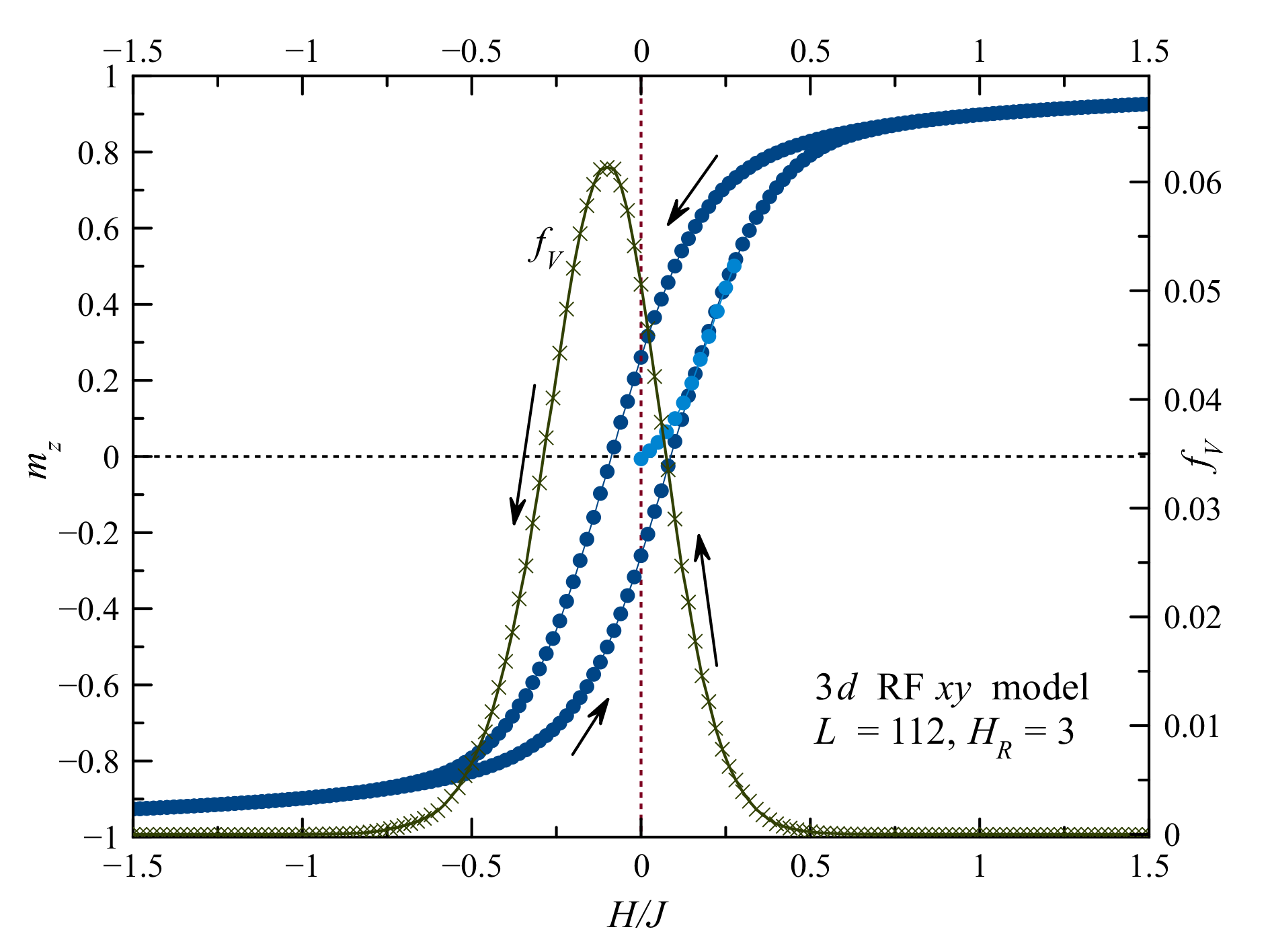
For a strong random field, such as $H_{R}=3$ in Fig. 18, hysteresis curves have a standard form. The irreversibility is related to the energy barriers at the atomic scale that changes the systems’ vorticity. The relation between vorticity and hysteresis is clearly seen in the Fig. 18. In the course of the reversal the magnetization $m$ decreases down to zero and then grows in magnitude again (not shown).

Fig. 19 shows hysteresis curves of a random-field $xy$ magnet for $H_{R}=1.5$ and $L=216$. The initial magnetization curve that begins with $m_{z}=0$ at $H=0$ has a rather small slope, in a striking disagreement with large zero-field susceptibility that follows from the Green-function method, Eq. (52). This high rigidity of the vortex-glass state is due to the pinning of vortices that Imry-Ma scenario does not account for.

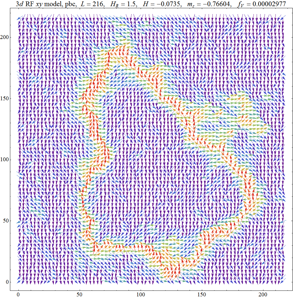
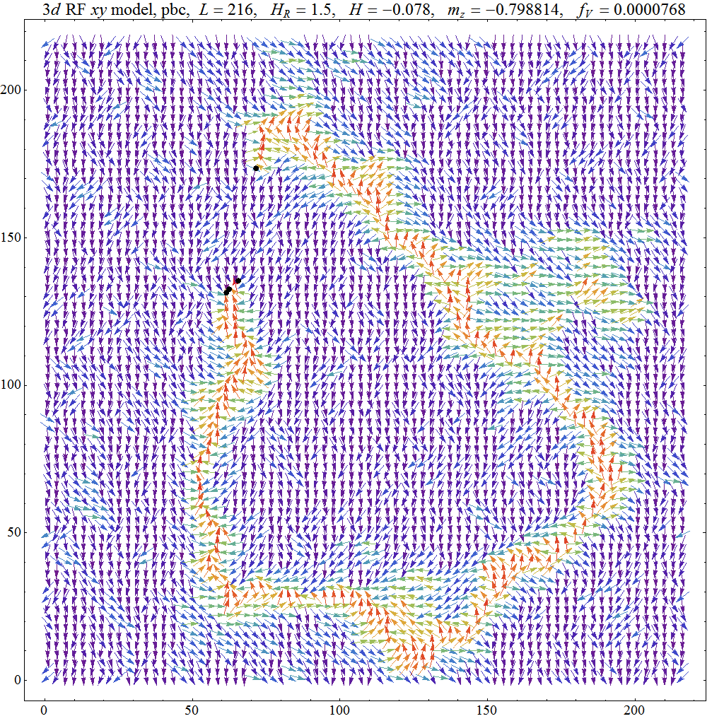
There is a large $m$ at $H=0$ along the $H$-down branch in Fig. 19 that does not depend strongly on the system size, which is in accord with Fig. 7. While the dependence of $m_{z}$ on $H$ along the hysteresis curve is rather steep at small fields, it is nearly smooth and has only small Barkhausen jumps (not seen in the figure), with the slope in the ball park of that given by Eq. (52). The magnetization of the sample does not rotate as a whole from positive to negative values of $m_{z}$. Instead, on average, the deviations of spins to the right and to the left from the positive $z$ direction in different regions of space increase smoothly as $H$ grows negative. In the process of spin reversal the regions with right and left spin deviations occupy rather large volumes separated by transient regions where spins are still directed in the positive $z$ direction. Such transient regions form walls of topological origin, see the cross-section of the sample in Fig. (20). They are pinned by the random field.

As the magnetization reversal proceeds along the hysteresis curve, the walls rapture, with the raptured area bounded by the vortex loop, as shown in Fig. 21. The loops then grow and eat the walls away, completing the reversal. This happens at $H=-H_{V}\approx 0.075$ in Fig. 19, where $m_{z}$ has a shoulder and vorticity has a peak. Such a behavior is typical for the $xy$ random magnet of size large compared to the ferromagnetic correlation length. Systems of smaller sizes typically switch their magnetization via rotation as a whole that leads to a jump from positive to negative values at a coercive field. This behavior is similar to that of a single-domain magnetic particle.

For $H>-H_{V}$, the upper hysteresis branch is quasi-reversible: Removing the field leads to partial restoration a large magnetization of the ferromagnetic state in $H=0$, which can interpreted as a memory effect. The simulated relaxation curves are shown in Fig. 22. The recovery happens because the ferromagnetic state with spin walls exhibits elasticity. As the field is reversed, it stores energy and tends to return to the initial state when the stress due to the opposite field is removed. This behavior is a good evidence of the stability of the ferromagnetic state. The incomplete restoration of the magnetization in this experiment should be due to energy barriers not related to vortices.

Figure 22: Magnetization recovery from the quasi-reversible branch of the hysteresis curve ($H>-H_{V}$ in Fig. 19), computed after setting $H=0$. The red curve corresponding to the initial value $m_{z}=-0.8$ does not go into the positive region because this initial state is beyond the quasi-reversible branch and has a large vorticity.

Figure 23: Energies of vortex-free ferromagnetic states (local energy minima) obtained by magnetization recovery of the type shown in Fig. 22. The rightmost state is obtained by relaxation from any state with $m\gtrsim 0.7$.

Figure 24: Energies of the states created by the external field $H$ vs $m_{z}$ (with the energy due to $H$ subtracted). The lowest-energy state corresponds to $m_{z}=0$ for $H_{R}\gtrsim 2.6$ and to $m_{z}>0$ for $H_{R}\lesssim 2.6$.

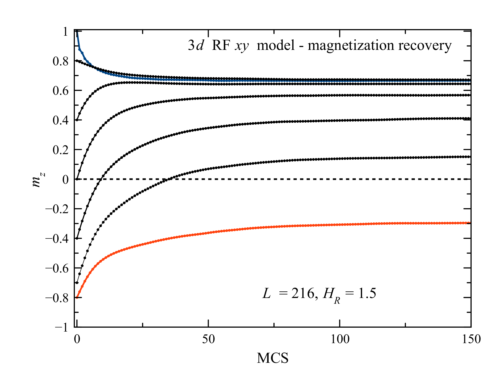
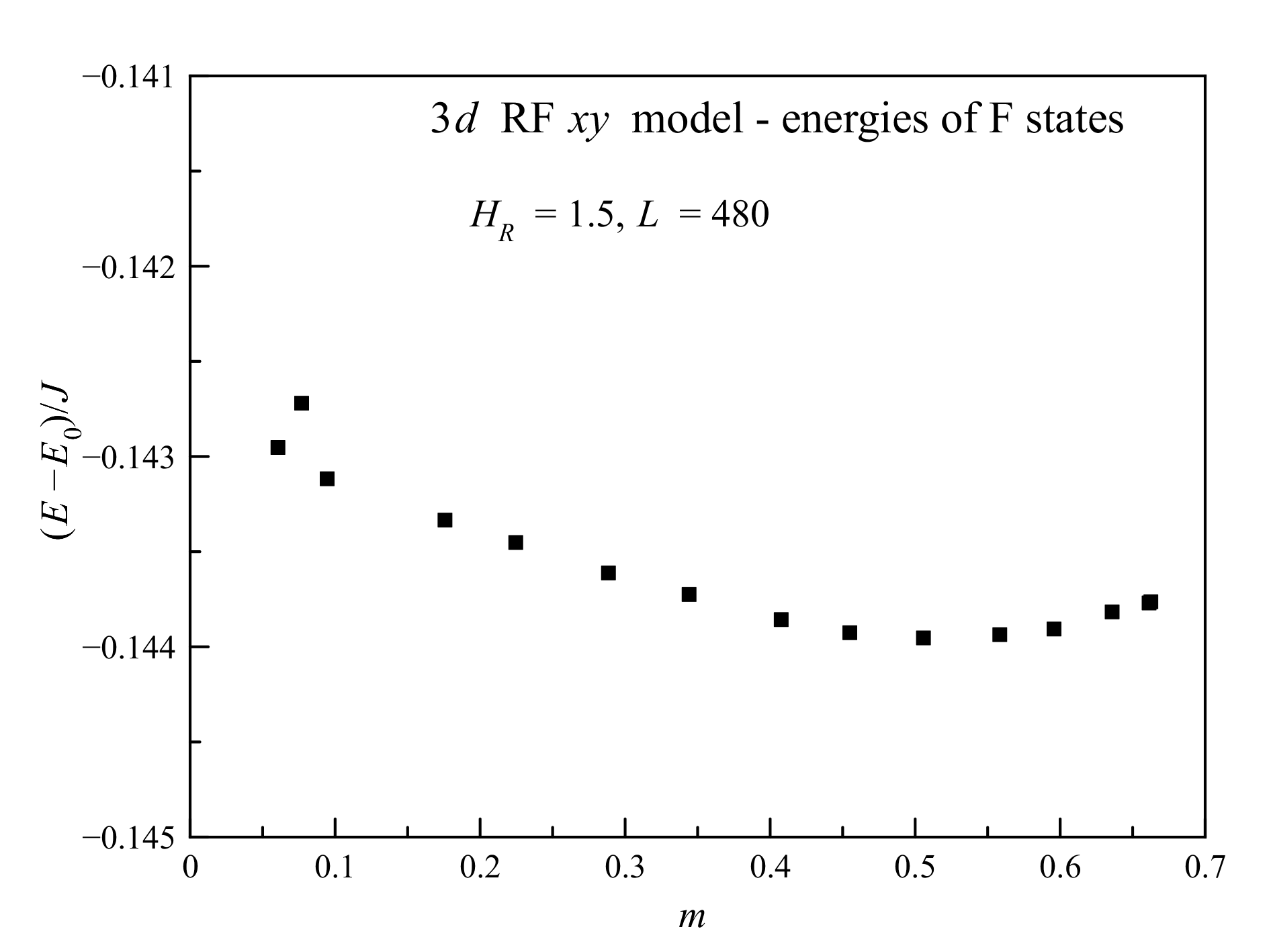
The magnetization-recovery experiment provides an access to more ferromagnetic states than just relaxation from a collinear state. Because of small barriers there is a big number of metastable ferromagnetic states that differ by energy and magnetization $m$, shown in Fig. 23. States with smaller $m$ occur due to relaxation from states with smaller $m_{z}$ in the upper hysteresis branch in Fig. 19. This is also seen in Fig. 22. The rightmost state in Fig. 23 is obtained by relaxation from any state with $m\gtrsim 0.7$ because there are no local energy minima in this range. There is a significant interval of $m$ values in the ferromagnetic states in Fig. 23, all having very close energies, in contrast with much larger energy differences between vortex-glass states in Fig. 16. One can clearly see that the lowest-energy state is at $m\approx 0.5$, a value that varies a bit depending on the random field realization. The energy values in Fig. 23 are comparable to those of the ferromagnetic states for $L=216$ in Fig. 16 and the states in Fig. 10.

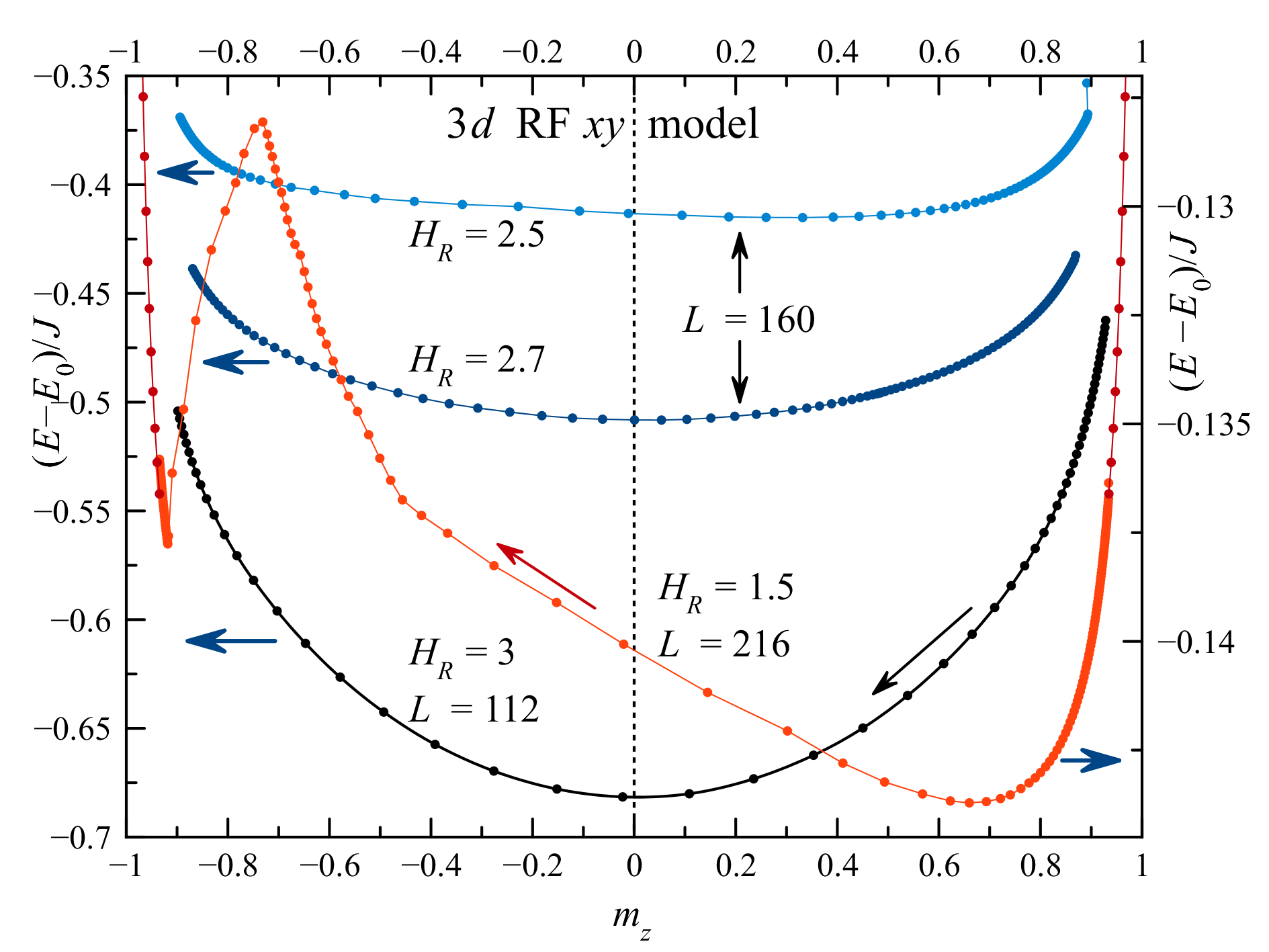
Another method of accessing the energies of the states vs their magnetization is to plot the energy obtained in the computation of the hysteresis (with the energy due to the external magnetic field $H$ subtracted) vs $m_{z}$. In this way one can access not only local energy minima, as in Fig. 23 but also the energies of all unstable states supported by the external field. Fig. 24 shows the computed energies for different values of $H_{R}$. A striking feature is the transition between the energy minimum at $m=0$ to an energy munimum at $m>0$ on $H_{R}$ that occurs at $H_{R}\approx 2.6$. One can see that for $H_{R}=1.5$ the results are very close to those for the local energy minima in Fig. 23 but also contain unstable states with $m\gtrsim 0.7$. Suppression of ferromagnetic states at large $H_{R}$ was already seen in Fig. 13. The energy maximum at $m_{z}\approx-0.8$ corresponds to the shoulder at this $m_{z}$ in Fig. 19. On decreasing $H_{R}$, its increasing part is due to the energy input into compressed spin walls while its decreasing part and it is due to rapture of spin walls by vortex loops.

V.9 Ordering by decreasing rotating field

Figure 25: Magnetization vs decreasing magnitude of a rotating field $\mathbf{H}$

Figure 26: Components of the magnetization vector $\mathbf{m}$ in the rotating-field experiment

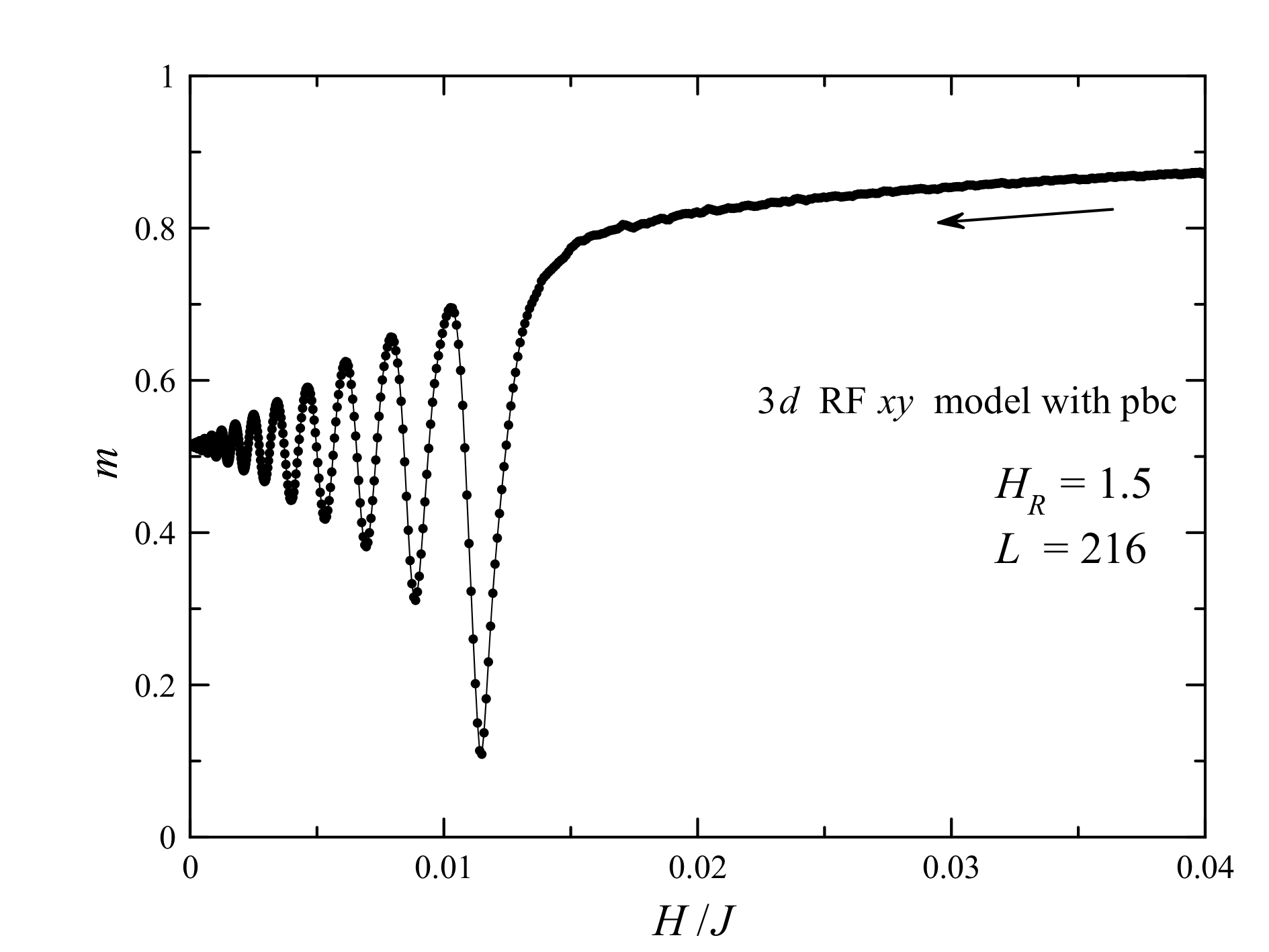
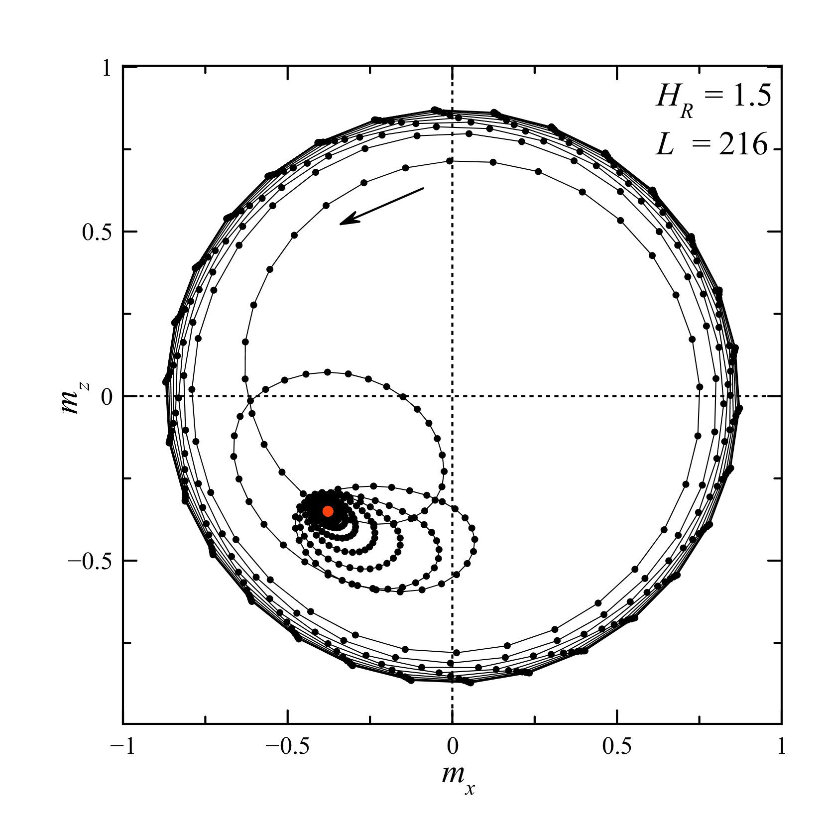
Another type of numeric experiment showing ferromagnetic ordering is relaxation in the presence of a rotating external field $\mathbf{H}$ with the magnitude slowly decreasing to zero. This is a version of the method of stimulated annealing that helps the system to overcome barriers preventing it from relaxing to states with a lower energy. If there were states with a small or zero magnetization having a lower energy that in our other numerical experiments, these states were likely to be reached by this method.

Numerical results shown in Figs. 25 and 26 show that also in the decreasing rotating field experiment ferromagnetically ordered states are reached. For the field magnitude $H$ large enough, the direction of $\mathbf{m}$ follows that of $\mathbf{H}$, while both $H$ and $m$ are decreasing. As $H$ goes below 0.015 (see Fig. 25), direction of $\mathbf{m}$ decouples from that of $\mathbf{H}$ and, after oscillations around an energy minimum corresponding to a significant value of $m$, the system reaches this energy minimum. In the above numerical experiment, the final magnetization value is $m=0.5148$. It turns out that our method leads to the energy values very close to those of Fig. 23. Thus, no states with a smaller $m$ and lower energy have been found, that again proves robustness of the ferromagnetically ordered state.

In another type of numerical experiment, a field slowly oscillating parallel to a fixed direction with the amplitude slowly decreasing to zero had been applied. Here one could obtain states with a small magnetization. However, the energy of such states was higher than the energy of the F state because of the vorticity generated by rapturing spin walls, see Sec. V.8.

V.10 Correlation functions

Figure 27: Correlation functions of the $3d$ RF $xy$ model in the vortex glass state obtained starting from random initial conditions. Natural (top) and scaled (bottom) presentations. $R_{V}$ is given by Eq. (72).

Figure 28: Correlation functions of the $3d$ RF $xy$ model in the ferromagnetic state obtained starting from collinear initial conditions.

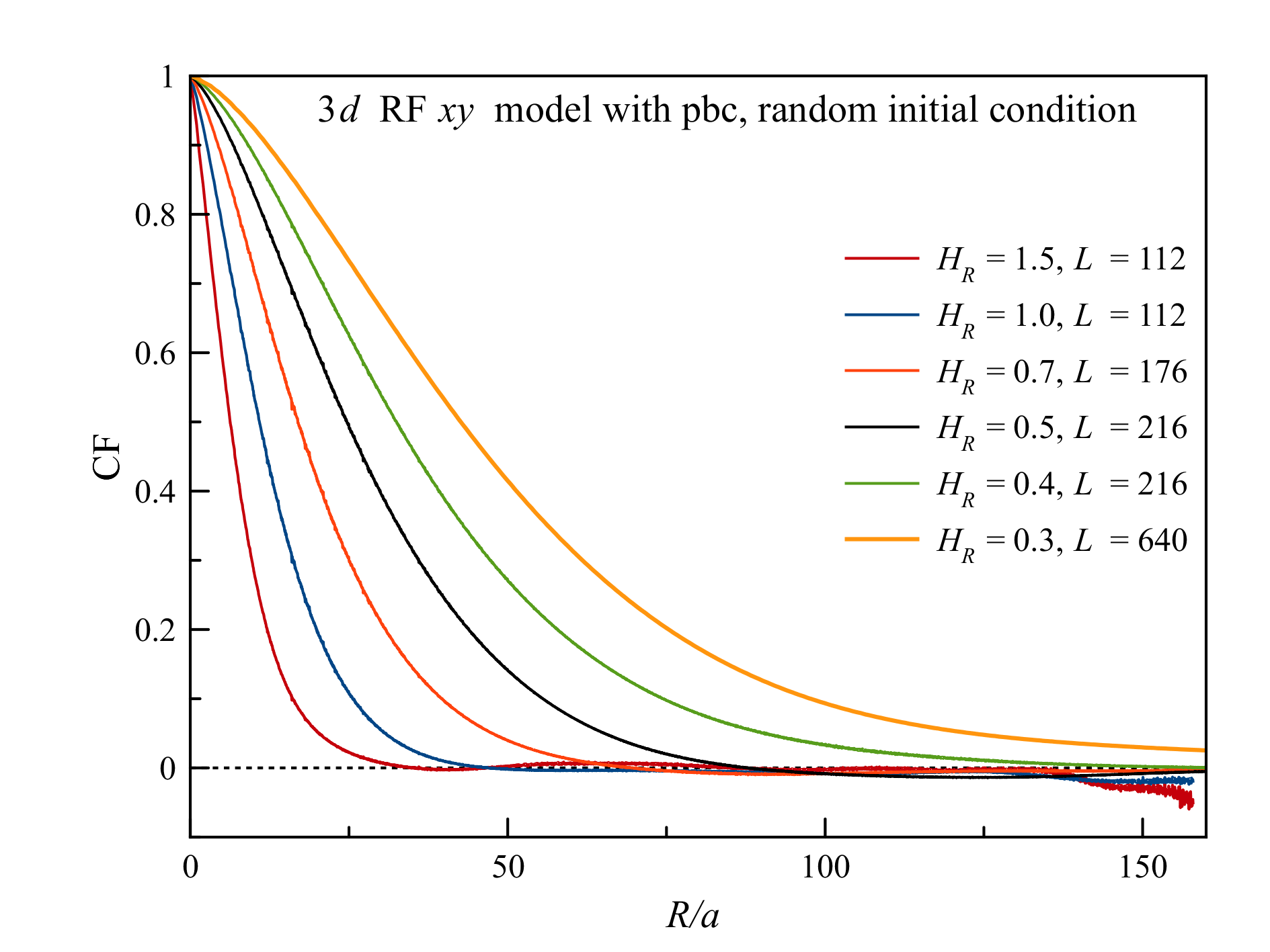
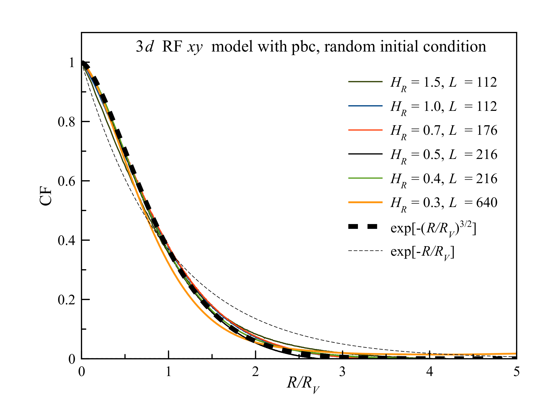
We have computed correlation functions in the energy minima of our system that we have found by our relaxation algorithm. After computing CFs we averaged them over directions of $\mathbf{R}\equiv{\bf r}_{1}-{\bf r}_{2}$.

In the vortex-glass state obtained from random initial conditions, correlation functions shown in Fig. 27 decay to zero but their form and correlation radius is different from Eqs. (26) and (23). The results can be fitted by the stretched exponential

$$\langle{\bf s}({\bf r}_{1})\cdot{\bf s}({\bf r}_{2})\rangle=s^{2}e^{-(|{\bf r}_{1}-{\bf r}_{2}|/R_{V})^{3/2}},\quad R_{V}\simeq 14\left(Js/H_{R}\right)^{1.2}.$$ (72)

Note that the dependence of $R_{V}$ on $H_{R}$ is much weaker than $R_{f}\propto 1/H_{R}^{2}$ of Eq. (23) and thus $R_{V}\ll R_{f}$ at small $H_{R}$. Using the vorticity dependence of Eq. (69), one can express the VG correlation length $R_{V}$ as

$$R_{V}\simeq 0.6/f_{V}^{1/2},$$ (73)

c.f. Eq. (70). This dependence is in agreement with the $2d$ nature of vortices discussed below Eq. (70).

If the initial state is collinear and $H_{R}$ is not too large, the correlation functions have plateaus at large distances. At $R\lesssim R_{f}$ they exactly follow Eq. (26). The results for our largest size $L=800$ are presented in Fig. 28. For $H_{R}=1$ and 1.5 there is enough self-averaging and we show correlation functions obtained for only one random-field realization. They have well-defined plateaus with small fluctuations. For $H_{R}=0.7$, correlation functions obtained with one random-field realization are too bumpy and averaging over realizations is needed. The bumps at $R=800$ and $\sqrt{2}\times 800$ are artifacts of periodic boundary conditions. The length of the plateaus show that the large magnetization in the ferromagnetic state is not a fluctuational magnetization.

The perfect plateau for $H_{R}=2.5$ shows that the appreciable vorticity $f_{V}=0.01766$ in this state does not yet disrupt ferromagnetic order at long distances. This should be the consequence of vortices forming small closed loops such as in Fig. 12(top). Meanwhile, one can expect that even a small concentration of vortex lines that go through the whole sample, as is the case in the vortex-glass state, see Fig. 12(bottom), will destroy the long-range order.

VI The Imry-Ma argument and vortices

Surprising robustness of the ferromagnetic state found in our different calculation requires an explanation. According to the Imry-Ma scenario, starting from collinear state, spins would relax towards directions of the random field averaged over correlated regions of linear size $R_{f}$, so that the magnetization would go to zero if $R_{f}$ is small compared to the size of the system. In our computations we indeed observe a fast initial disordering but then the magnetization stops to decrease at an appreciable value, Figs. 2 and 3. What could be the factor that prevents it from relaxing to zero?

Figure 29: (Top) Domains of positive and negative $h_{x}(\mathbf{r})$ in a $xy$ plane. (Bottom) Singularities at the crossings of domain boundaries for $h_{x}(\mathbf{r})$ and $h_{y}(\mathbf{r})$ in a $xy$ plane.

Figure 30: Formation of vortices and antivortices at the crossings of domain boundaries for $h_{x}(\mathbf{r})$ and $h_{y}(\mathbf{r})$.

The answer to this question seems to be that the magnetization cannot smoothly follow the average random field without the formation of vortices in $2d$ and vortex loops in $3d$. The latter cost energy that prevents relaxation towards a completely disordered state. Thus ferromagnetically ordered state is topologically protected.

This can be demonstrated by considering the average of the random field over the correlated region around each point $\mathbf{r}$, the so-called moving average, for instance,

$$\mathbf{\bar{h}}(\mathbf{r})=\frac{1}{V_{f}}\intop_{|\mathbf{r}^{\prime}|\leq R_{f}}d^{d}\mathbf{r}^{\prime}\mathbf{h}(\mathbf{r}^{\prime}+\mathbf{r}),$$ (74)

where $V_{f}$ is the correlated volume, $V_{f}=\left(4\pi/3\right)R_{f}^{3}$ in $3d$. This is exactly a mathematical implementation of the original Imry-Ma argument. The averaged random field $\mathbf{\bar{h}}(\mathbf{r})$ describes a disorder correlated at length $R_{f}$. Since its components $\bar{h}_{x}(\mathbf{r})$ and $\bar{h}_{y}(\mathbf{r})$ are sums of many random variables, they have a Gaussian distribution at any point $\mathbf{r}$ and are statistically independent. Spin field in the Imry-Ma state, aligned with $\mathbf{\bar{h}}(\mathbf{r})$, should be of the form

$$\mathbf{s}_{\mathrm{IM}}(\mathbf{r})=\frac{\mathbf{\bar{h}}(\mathbf{r})}{\left|\mathbf{\bar{h}}(\mathbf{r})\right|}.$$ (75)

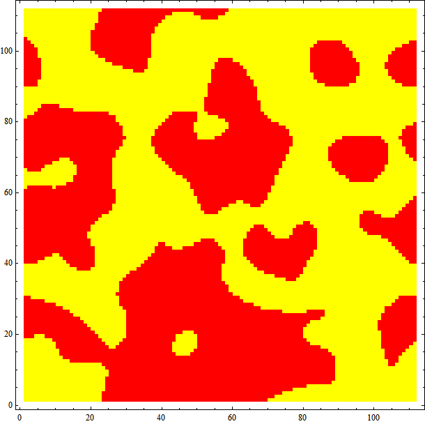
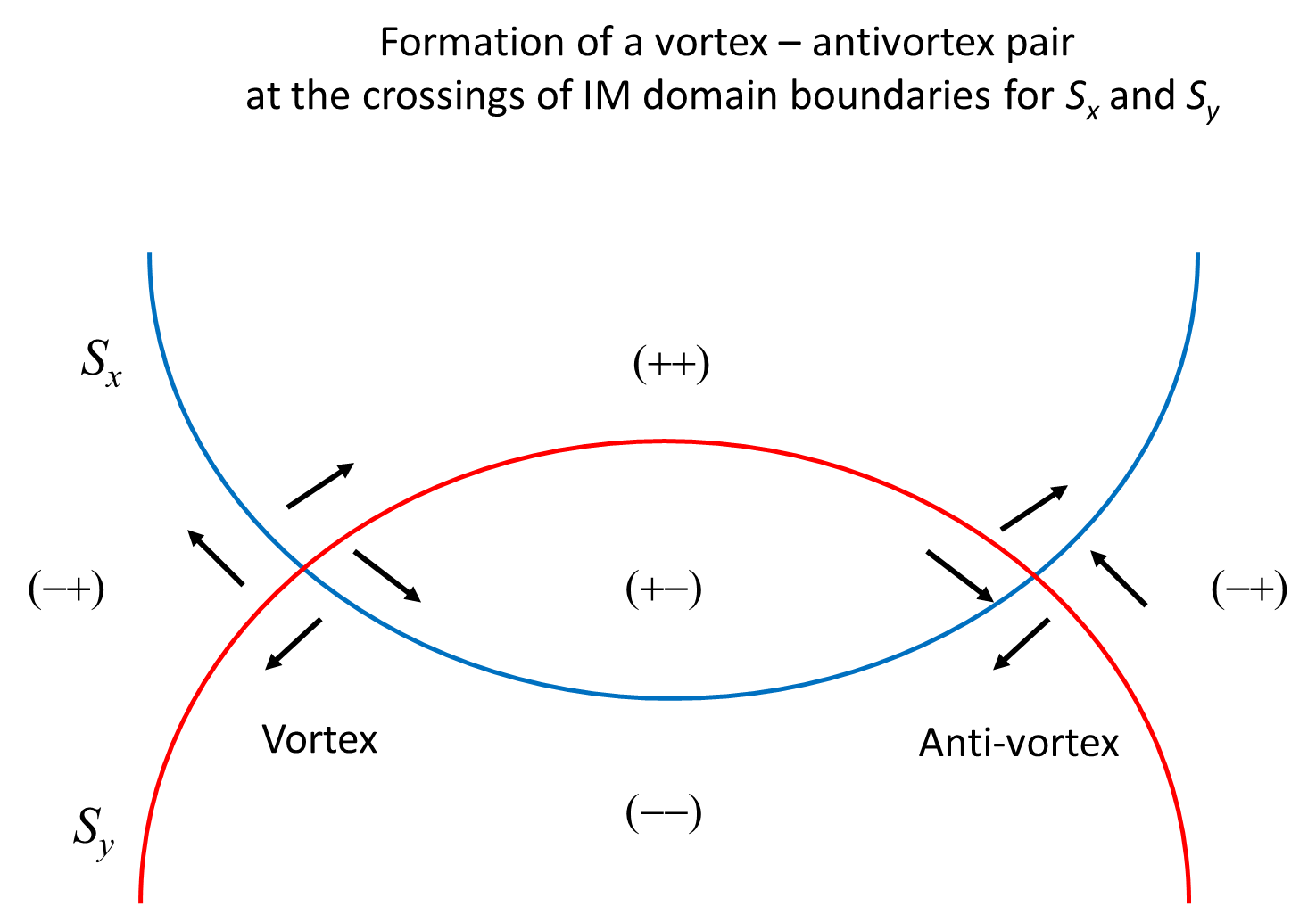
Now, it can be shown that such defined spin field has singularities. This happens when $\left|\mathbf{\bar{h}}(\mathbf{r})\right|=0$, that is, both components of $\mathbf{\bar{h}}(\mathbf{r})$ turn to zero. Regions of positive and negative $s_{x}(\mathbf{r})$ in a $xy$ plane, generated by Eq. (75) are shown on Fig. 29. The areas of positive and negative $s_{x}(\mathbf{r})$ are on average the same and the boundaries between domains are random lines shown in Fig. 29(top). Domain boundaries for $s_{y}(\mathbf{r})$ are also random lines statistically independent from the former. Thus domain boundaries for $s_{x}(\mathbf{r})$ and $s_{y}(\mathbf{r})$ will cross at some points, as shown in Fig. 29(bottom). At these points vortices or antivortices will be generated because of the denominator in Eq. (75), as illustrated in Fig. 30. In $3d$ there will be vortex loops that cost much more energy than a vortex in $2d$.

Let us now estimate the energy gain in the IM state with vortices. There is about one vortex per IM domain with size $R_{f}$, having the energy

$$E_{V}\sim Js^{2}\left(\frac{R_{f}}{a}\right)\ln\left(\frac{R_{f}}{a}\right).$$ (76)

The corresponding exchange energy per spin is

$$E_{\mathrm{ex}-V}\sim Js^{2}\left(\frac{a}{R_{f}}\right)^{2}\ln\left(\frac{R_{f}}{a}\right)$$ (77)

that should replace the second term in Eq. (11). Minimization with respect to $R_{f}$ in that expression gives

$$R_{f}\sim a\left(\frac{Js}{h}\right)^{2}\ln^{2}\left(\frac{Js}{h}\right)$$ (78)

that is longer than the IM correlation radius because of the large lorarithm. The corresponding energy gain

$$E-E_{0}\sim-Js^{2}\left(\frac{h}{Js}\right)^{4}\left[\ln\left(\frac{Js}{h}\right)\right]^{-3}\sim\frac{\Delta E_{IM}}{\ln^{3}(Js/h)}$$ (79)

is the IM energy gain divided by a large logarithmic term.

On the other hand, the ferromagnetic state we have found numerically can be understood as an incompletely disordered IM state, in which the energy gain is $\Delta E_{IM}$ reduced by a numerical factor of order one rather than by a large logarithmic term. The energy of this ferromagnetic state should be lower than that of the IM state with vortices, in accordance with our numerical results (see, e.g., Figs. 15 and 16). The rapid relaxation out of the collinear state followed by a plateau in Figs. 2 and 3 can be explained as follows. Spins are readily relaxing in the direction of the net RF in the regions of linear size $R_{f}$ until their further rotation toward the totally disordered IM state requires creation of vortices. As the latter costs energy, relaxation stops at this point.

Of course, there is a non-zero probability that the random field at the location of the vortex is vortex-like and almost parallel to the spin field. In this case the energy gain from the vortex will be significantly higher. However, since the Imry-Ma state in which the spin field follows the direction of the average local random field is unique for every choice of the correlated volume $V_{f}$, so should be the positions of the vortices. The fraction of the lucky vortices mentioned above is determined by the probability of the corresponding lucky configuration of the random field, which is small. Consequently, it cannot affect the above argument .

VII Discussion

We have studied states of local energy minima of the random-field $xy$ model focusing on weak random fields. The minimal random-field value $h\equiv H_{R}$ in our work is defined by $h/J=0.3$, see Fig. 27. This should be considered weak for the following reason. In the cubic lattice each spin has six nearest neighbors that are nearly collinear for small $h$, the exchange field is $J_{0}\equiv 6J$. Thus, physically it makes more sense to consider the dimensionless parameter $h/J_{0}$ that in our computations has the minimal value $h/J_{0}=0.05$ being manifestly small. In terms of $J_{0}$ formulas of the LIM theory do not contain large numbers. For instance, $R_{f}$ in Eq. (23) can be rewritten as $R_{f}/a=(4\pi/9)(J_{0}s/h)^{2}$.

Computations have been performed on lattices up to $1000\times 1000\times 1000$ spins. Our main finding is that completely disordered ($m\cong 0$) states are dominated by vortices and have higher energy than vortex-free ferromagnetically ordered states. There are unsurpassable energy barriers between different states even in the case of a weak random field because switching between different spin configurations involves large groups of correlated spins. This makes the magnetic states depend strongly on the initial conditions. At first glance this may appear conceptually similar to the behavior of a conventional ferromagnet with pinning of domain walls. Prepared with random orientations of spins, it would freeze in a state with small magnetic domains and high energy due to many domain walls. In a similar fashion, the random-field magnet freezes in a high-energy state due to many vortices pinned by the random field. When prepared with collinear spins, the conventional ferromagnet would remain in a magnetized state because pinning prevents domain walls from proliferating into the sample and achieving the ground state with zero total magnetization. Similarly, the random-field magnet prepared with collinear spins relaxes to a state with non-zero magnetic moment.

There is an essential difference between the two systems though. While the conventional ferromagnet tends to relax toward an $m=0$ state via diffusion of domain walls out of local energy minima, the random-field magnet in our computations does not have this tendency to relax to the zero-magnetization state out of the magnetized state. In fact the energies of zero-magnetization states found in our various types of computations are always higher than the energies of magnetized states. One possibility is that the zero-magnetization state is not the ground state. Another possibility is that there are energy barriers to relaxation out of the magnetized state that involve collective behavior of large volumes of spins and they are actually greater for a weaker random field. This would be very different from shallow local energy barriers for the diffusion of domain walls in conventional ferromagnets.

The bottom line of our analysis is that the Imry-Ma state in which the system breaks into finite-size domains providing zero total magnetic moment is impossible without formation of vortex loops. They become very long and possess very large energy when the random field becomes very small. This makes the barriers associated with the formation of the zero-magnetization state unsurpassable at any temperature even in the limit of weak random field. The above argument is based upon $h$-dependence of $R_{f}$ and it stands as long as $R_{f}$ is small compared to the size of the system. One can ask how close the vortex-glass state is to the Imry-Ma state. To address this question, for $H_{R}=1.5$ we have created an Imry-Ma state of Eq. (75) and let it relax. As the result, the vorticity decreased from $f_{V}\approx 0.008$ in the Imry-Ma state to $f_{V}\approx 0.0006$ in the vortex-glass state. This means that the system tries to annihilate vortices to reduce its energy but it cannot do it completely because some vortices are pinned. Similar conclusion regarding dislocations in two-dimensional pinned flux lattices has been reached in Ref. Fisher-PRL99, .

On the other hand, it must be stressed that the ground state of the system was not systematically searched for, and, moreover, it is of little relevance in glassy systems. A single vortex loop going across the whole sample will totally destroy magnetic order while its excess energy, as well as its vorticity, will be vanishingly small. It cannot be excluded that such type of states has the lowest possible energy. However, these states are exotic and they were not studied here. Consequently, we cannot rule out the existence a completely disordered vortex-free ground state in our computations. However, finding such a state may require a special initial condition or a more sophisticated numerical argorithm anticipating the result.

It is generally believed, see, e.g., Refs. Fisher-PRL1997, ; Nat-review, , that in the presence of quenched randomness the elastic interactions, like the ones in the atomic or vortex lattices, or exchange in spin lattices, provide the elastic-glass ground state that is characterized by the power law decay of correlations at large distances. We have not found such a behavior for the random-field $xy$ spin model in three dimensions. The relation between that model and randomly pinned flux lattices in superconductors has been discussed in some detail in Ref. Gingras-Huse-PRB1996, . The role of topological defects in flux lattices is played by dislocations as compared to vortices in spin models. Large areas of defect-free flux lattices have been observed in experiment, see, e.g., Ref. Klein-Nature2001, . When analyzing such experiments, one should remember, however, that for weak disorder the correlation length in $3d$ can be very large, making it difficult to distinguish large defect-free slightly disordered domains from the Bragg glass. While it is possible that some of the conclusions of this paper apply to pinned flux lattices the latter requires a separate study because the two models have different symmetry and different kinds of interaction with the random field.

VIII Acknowledgements

The authors acknowledge useful discussions with Joseph Imry, Thomas Nattermann, and Valerii Vinokur. This work has been supported by the U.S. Department of Energy through Grant No. DE-FG02-93ER45487.

References

- (1) A. I. Larkin, Sov. Phys. JETP 31, 784 (1970).
- (2) K. B. Efetov and A. I. Larkin, Sov. Phys. JETP 72, 2350 (1977).
- (3) E. M. Chudnovsky, W. M. Saslow and R. A. Serota, Phys. Rev. B 33, 251 (1986).
- (4) Y. Imry and S.-k. Ma, Phys. Rev. Lett. 35, 1399 (1975).
- (5) M. Aizenman and J. Wehr, Phys. Rev. Lett. 62, 2503 (1989).
- (6) M. Aizenman and J. Wehr, Commun. Math. Phys. 130, 489 (1990).
- (7) J. D. Patterson, G. R. grusalski, and D. J. Sellmyer, Phys. Rev. B 18, 1377 (1978).
- (8) R. Pelcovits, E. Pytte, and J. Rudnick, Phys. Rev. Lett. 40, 476 (1978)
- (9) A. Aharony and E. Pytte, Phys. Rev. Lett. 45, 1583 (1980).
- (10) S. Fishman and A. Aharony, J. Phys. C: Solid State Phys. 12, L729 (1979).
- (11) D. S. Fisher, Phys.Rev. B 31,7233 (1985).
- (12) G. Blatter, M. V. Feigel’man, V. B. Geshkenbein, A.I. Larkin, and V. M. Vinokur, Rev. Mod. Phys. 66, 1125 (1994).
- (13) K. Binder and A. P. Young, Rev. Mod. Phys. 58, 801 (1986).
- (14) E. M. Chudnovsky, Phys. Rev. B 43, 7831 (1991).
- (15) E. M. Chudnovsky, Phys. Rev. Lett. 103, 137001 (2009).
- (16) J. L. Cardy and S. Ostlund, Phys. Rev. B 25, 6899 (1982).
- (17) J. Villain and J. F. Fernandez, Z. Phys. B - Condens. Matter 54, 139 (1984).
- (18) T. Nattermann, Phys. Rev. Lett. 64, 2454 (1990).
- (19) J. Kierfield, T. Nattermann, and T. Hwa, Phys. Rev. B 55, 626 (1997).
- (20) S. E. Korshunov, Phys. Rev. B 48, 3969 (1993).
- (21) T. Giamarchi and P. Le Doussal, Phys. Rev. Lett. 72, 1530 (1994).
- (22) T. Giamarchi and P. Le Doussal, Phys. Rev. B 52, 1242 (1995).
- (23) P. Le Doussal amd K. J. Wiese, Phys. Rev. Lett. 96, 197202 (2006).
- (24) P. Le Doussal, Phys. Rev. Lett. 96, 235702 (2006).
- (25) A. A. Middleton, P. Le Doussal, and K. J. Wiese, Phys. Rev. Lett. 98, 155701 (2007).
- (26) S. Bogner, T. Emig, A. Taha, and C. Zeng, Phys. Rev. B 69, 104420 (2004).
- (27) H. Orland and Y. Shapir, Europhys. Lett. 30, 203 (1995).
- (28) T. Garel, G. Lori, and H. Orland, Phys. Rev. B 53, R2941 (1996).
- (29) R. Dickman and E. M. Chudnovsky, Phys. Rev. B 44, 4397 (1991).
- (30) B. Dieny and B. Barbara, Phys. Rev. B 41, 11549 (1990).
- (31) M. J. P. Gingras and D. A. Huse, Phys. Rev. B 53, 15193 (1996).
- (32) T. Nattermann and S. Scheidl, Adv. of Phys. 49, 607 (2000).
- (33) C. Zeng, A. A. Middleton, and Y. Shapir, Phys. Rev. Lett. 77, 3204 (1996).
- (34) H. Rieger and U. Blasum, Phys. Rev. B 55, R7394 (1997).
- (35) M. Itakura, Phys. Rev. B 68, 100405(R) (2003).
- (36) M. Itakura and C. Arakawa, Prog. Theor. Phys. Suppl. No. 157, 136 (2005).
- (37) D. Fisher, Phys. Rev. Lett. 78, 1964 (1997).
- (38) R. Fisch, Phys. Rev. B 52, 12512 (1995); ibid 55, 8211 (1997); ibid 57, 269 (1998); ibid 62, 361 (2000); ibid 76, 214435 (2007); ibid 79, 214429 (2009).
- (39) A. Perret, Z. Ristivojevic, P. Le Doussal, G. Schehr, and K. J. Wiese, Phys. Rev. Lett. 109, 157205 (2012).
- (40) S. Adler, Phys. Rev. D 23, 2901 (1981).
- (41) Kun Chen and D. P. Landau, Phys. Rev. B 49, 3266 (1994).
- (42) J. M. Ziman, Models of Disorder (Cambridge University Press, Cambridge, England, 1979).
- (43) C. Zeng, P. L. Leath, and D. S. Fisher, Phys. Rev. Lett. 82, 1935 (1999).
- (44) T. Klein, I. Joumard, S. Blanchard, J. Marcus, R. Cubitt, T. Giamarchi, and P. Le Doussal, Nature 413, 404 (2001).