Knowledge-Aided STAP Using Low Rank and Geometry Properties

Abstract

This paper presents knowledge-aided space-time adaptive processing (KA-STAP) algorithms that exploit the low-rank dominant clutter and the array geometry properties (LRGP) for airborne radar applications. The core idea is to exploit the fact that the clutter subspace is only determined by the space-time steering vectors, redwhere the Gram-Schmidt orthogonalization approach is employed to compute the clutter subspace. Specifically, for a side-looking uniformly spaced linear array, the algorithm firstly selects a group of linearly independent space-time steering vectors using LRGP that can represent the clutter subspace. By performing the Gram-Schmidt orthogonalization procedure, the orthogonal bases of the clutter subspace are obtained, followed by two approaches to compute the STAP filter weights. To overcome the performance degradation caused by the non-ideal effects, a KA-STAP algorithm that combines the covariance matrix taper (CMT) is proposed. For practical applications, a reduced-dimension version of the proposed KA-STAP algorithm is also developed. The simulation results illustrate the effectiveness of our proposed algorithms, and show that the proposed algorithms converge rapidly and provide a SINR improvement over existing methods when using a very small number of snapshots.

I Introduction

Space-time adaptive processing (STAP) is considered to be an efficient tool for detection of slow targets by airborne radar systems in strong clutter environments [1, 2, 3, 4]. However, due to the very high degrees of freedom (DoFs), the full-rank STAP has a slow convergence and requires about twice the DoFs of the independent and identically distributed (IID) training snapshots to yield an average performance loss of roughly $3$dB [1]. In real scenarios, it is hard to obtain so many IID training snapshots, especially in heterogeneous environments. Therefore, it is desirable to develop STAP techniques that can provide high performance in small training support situations.

Reduced-dimension and reduced-rank methods have been considered to counteract the slow convergence of the full-rank STAP [1, 2, 3, 4, 5, 6, 7, 8, 9, 26, 28, 27]. These methods can reduce the number of training snapshots to twice the reduced dimension, or twice the clutter rank blueif we assume that the degrees of freedom of the reduced dimension correspond to the rank of the clutter. The parametric adaptive matched filter (PAMF) based on a multichannel autoregressive model [29] provides another alternative solution to the slow convergence of the full-rank STAP. Furthermore, the sparsity of the received data and filter weights has been exploited to improve the convergence of a generalized sidelobe canceler architecture in [30]. However, it still fundamental for radar systems to improve the convergence performance of STAP algorithms or reduce their required sample support in heterogeneous environments because the number of required snapshots is large relative to those needed in IID scenarios.

Recently developed knowledge-aided (KA) STAP algorithms have received a growing interest and become a key concept for the next generation of adaptive radar systems [32, 33, 34, 35, 36, 37, 38, 42, 43, 44, 45, 39, 40, 41]. The core idea of KA-STAP is to incorporate prior knowledge, provided by digital elevation maps, land cover databases, road maps, Global Positioning System (GPS), previous scanning data and other known features, to compute estimates of the clutter covariance matrix (CCM) with high accuracy [32, 33]. Among the previously developed KA-STAP algorithms, there is a class of approaches that exploit the prior knowledge of the clutter ridge to form the STAP filter weights in [42, 43, 44] and [45]. The authors in [42] introduced a knowledge-aided parametric covariance estimation (KAPE) scheme by blending both prior knowledge and data observations within a parameterized model to capture instantaneous characteristics of the cell under test (CUT). A modified sample matrix inversion (SMI) procedure to estimate the CCM using a least-squares (LS) approach has been described in [43] to overcome the range-dependent clutter non-stationarity in conformal array configurations. However, both approaches require the pseudo-inverse calculation to estimate the CCM and this often requires a computationally costly singular value decomposition (SVD) [42]. redAlthough two weighting approaches with lower computations are discussed in [42], they are suboptimal approaches to the LSE by the SVD and the performance of these approaches relative to the LSE by the SVD depends on bluethe radar system parameters, especially the array characteristics [42]. Moreover, the latter approach has not considered the situation when the prior knowledge has uncertainties. Under the assumption of the known clutter ridge in the angle-Doppler plane, the authors in [44] imposed the sparse regularization to estimate the clutter covariance excluding the clutter ridge. Although this kind of method can obtain a high-resolution even using only one snapshot, it requires the designer to know the exact positions of the clutter ridge resulting in being sensitive to the prior knowledge. Furthermore, the computational complexity caused by sparse recovery is expensive. A data independent STAP method based on prolate spheroidal wave functions (PSWF) has been considered in MIMO radar by incorporating the clutter ridge [45], where the computational complexity is significantly reduced compared with the approaches in [42] and [43]. However, it is highly dependent on the ideal clutter subspace and is not robust against clutter subspace mismatches.

In this paper, we propose KA-STAP algorithms using prior knowledge of the clutter ridge that avoid the pseudo-inverse calculation, require a low computational complexity, and mitigate the impact of uncertainties of the prior knowledge. redSpecifically, for a side-looking uniformly spaced linear array (ULA), the proposed method selects a group of linearly independent space-time steering vectors that can represent the ideal clutter subspace using prior knowledge of the dominant low-rank clutter and the array geometry properties (LRGP). The orthogonal bases of the clutter ideal subspace are computed by a Gram-Schmidt orthogonalization procedure on the selected space-time steering vectors. Two robust approaches to compute the STAP filter weights are then presented based on the estimated clutter subspace. To overcome the performance degradation caused by the redinternal clutter motion (ICM), we employ a covariance matrix taper (CMT) to the estimated CCM. The array calibration methods discussed in [42] can be applied to our proposed algorithm to mitigate the blueimpact of non-ideal factors, such as channel mismatching. Moreover, a reduced-dimension version of the proposed KA-STAP algorithm is devised for practical applications. Finally, simulation results demonstrate the effectiveness of our proposed algorithms.

The main contributions of our paper are:

(i) A KA-STAP algorithm using blueprior knowledge of the LRGP is proposed for airborne radar applications.

(ii) A KA-STAP combining CMT is introduced to counteract the performance degradation caused by ICM redand prior knowledge uncertainty, and a reduced-dimension version is also presented for practical applications. redFurthermore, the proposed algorithm provides evidence for the KAPE approach to directly use the received data and the calibrated space-time steering vectors (only the spatial taper without the temporal taper) to compute the assumed clutter amplitude.

(iii) A detailed comparison is presented to show the computational complexity of the proposed and existing algorithms.

(iv) A study and comparative analysis of our proposed algorithms including the impact of inaccurate prior knowledge and non-ideal effects on the SINR performance, the convergence speed and the detection performance with other STAP algorithms is carried out.

The work is organized as follows. Section II introduces the signal model in airborne radar applications. Section III details the approach of the proposed KA-STAP algorithms and also discusses the computational complexity. The simulated airborne radar data are used to evaluate the performance of the proposed algorithms in Section IV. Section V provides the summary and conclusions.

II Signal Model

The system under consideration is a side-looking pulsed Doppler radar with a redULA consisting of $M$ elements on the airborne radar platform, as shown in Fig.1. The platform is at altitude $h_{p}$ and moving with constant velocity $v_{p}$. The radar transmits a coherent burst of pulses at a constant pulse repetition frequency (PRF) $f_{r}=1/T_{r}$ , where $T_{r}$ is the pulse repetition interval (PRI). The transmitter carrier frequency is $f_{c}=c/\lambda_{c}$, where $c$ is the propagation velocity and $\lambda_{c}$ is the wavelength. The number of pulses in a coherent processing interval (CPI) is $N$. The received signal from the iso-range of interest is represented by a space-time $NM\times 1$ data vector ${\bf x}$.

redThe received space-time clutter plus noise return from a single range bin can be represented by [4]

$${\bf x}=\sum^{N_{a}}_{m=1}\sum^{N_{c}}_{n=1}\sigma_{m,n}{red}{{\bf v}(f_{s,m,n},f_{d,m,n})\odot{\boldsymbol{\alpha}}(m,n)}+{\bf n},$$ (1)

where ${\bf n}$ is the Gaussian white thermal noise vector with the noise power $\sigma^{2}_{n}$ on each channel and pulse; $N_{a}$ is the number of range ambiguities; $N_{c}$ is the number of independent clutter patches over the iso-range of interest; $f_{s,m,n}$ and $f_{d,m,n}$ are the redspatial and Doppler frequencies of the $mn$th clutter patch, respectively; red$\sigma_{m,n}$ is the complex amplitude for the $mn$th clutter patch; ${\boldsymbol{\alpha}}(m,n)={\boldsymbol{\alpha}}_{d}(m,n)\otimes{\boldsymbol{\alpha}}_{s}(m,n)$ is the space-time random taper vector characterizing the voltage fluctuation caused by bluenon-ideal factors, such as ICM and channel mismatch (where ${\boldsymbol{\alpha}}_{d}(m,n)$ and ${\boldsymbol{\alpha}}_{s}(m,n)$ are the temporal and spatial random tapers); and ${\bf v}(f_{s,m,n},f_{d,m,n})$ is the $NM\times 1$ space-time steering vector for a clutter patch with red$f_{s,m,n}$ and $f_{d,m,n}$.

Figure 1: Airborne radar geometry with a ULA antenna.

The space-time steering vector is given as the Kronecker product of the temporal and spatial steering vectors, ${\bf v}(f_{s,m,n},f_{d,m,n})={\bf v}_{t}(f_{d,m,n})\otimes{\bf v}_{s}(f_{s,m,n})$, which are given by [1]

$${\bf v}_{t}(f_{d,m,n})=[1,\cdots,\exp(j2\pi(N-1)f_{d,m,n})]^{T},$$ (2)

$${\bf v}_{s}(f_{s,m,n})=[1,\cdots,\exp(j2\pi(M-1)f_{s,m,n})]^{T},$$ (3)

where $()^{T}$ denotes the transposition operation, $f_{s,m,n}=\frac{d_{a}}{\lambda_{c}}\cos\theta_{m,n}\sin\phi_{m,n}$, $f_{d,m,n}=\frac{2v_{p}T_{r}}{\lambda_{c}}\cos\theta_{m,n}\sin\phi_{m,n}$, and $d_{a}$ is the inter-sensor spacing of the ULA. If we stack all clutter patches’ amplitudes into a vector

$${\boldsymbol{\sigma}}=[\sigma_{1,1},\cdots,\sigma_{1,N_{c}},\cdots,\sigma_{N_{a},1},\cdots,\sigma_{N_{a},N_{c}}]^{T},$$ (4)

redand assume there are no non-ideal factors, then the clutter plus noise received data denoted by (1) can be reddescribed as

$${\bf x}={\bf x}_{c}+{\bf n}={\bf V}{\boldsymbol{\sigma}}+{\bf n},$$ (5)

where ${\bf V}$ denotes the clutter space-time steering matrix, given by

$$\begin{split}{\bf V}=&[{\bf v}(\phi_{1,1},\theta_{1,1},f_{1,1}),\cdots,\\ &{\bf v}(\phi_{1,N_{c}},\theta_{1,N_{c}},f_{1,N_{c}}),\cdots,\\ &{\bf v}(\phi_{N_{a},1},\theta_{N_{a},1},f_{N_{a},1}),\cdots,\\ &{\bf v}(\phi_{N_{a},N_{c}},\theta_{N_{a},N_{c}},f_{N_{a},N_{c}})].\end{split}$$ (6)

Thus, the CCM based on (5) can be expressed as

$${\bf R}_{c}={\bf V}{\boldsymbol{\Sigma}}{\bf V}^{H},$$ (7)

where ${\boldsymbol{\Sigma}}=E[{\boldsymbol{\sigma}}{\boldsymbol{\sigma}}^{H}]$. Under the condition that the clutter patches are independent from each other, ${\boldsymbol{\Sigma}}={\rm diag}({\bf a})$, ${\bf a}=[a_{1,1},a_{1,2},\cdots,a_{N_{a},N_{c}}]^{T}$ and $a_{m,n}=E[|{\sigma}_{m,n}|^{2}]$ ($m=1,\cdots,N_{a}$, $n=1,\cdots,N_{c}$) for the statistics of the clutter patches. Here, $E[\cdot]$ denotes the expectation operator, ${\rm diag}({\bf a})$ stands for a diagonal matrix with the main diagonal taken from the elements of the vector ${\bf a}$ and $()^{H}$ represents the conjugate transpose of a matrix.

The optimal filter weight vector on maximizing the output SINR for the Gaussian distribution clutter which is given by the full-rank STAP processor can be written as [4]

$${\bf w}_{\rm opt}=\mu{\bf R}^{-1}{\bf s},$$ (8)

where $\mu$ is a constant which does not affect the SINR performance, ${\bf s}$ is the $NM\times 1$ space-time steering vector in the target direction, and ${\bf R}=E[{\bf x}{\bf x}^{H}]={\bf R}_{c}+\sigma^{2}_{n}{\bf I}$ is the clutter plus noise covariance matrix (${\bf I}$ is the identity matrix).

III KA-STAP Algorithms Using LRGP

In this section, we firstly review the method that estimates the CCM using a LS technique in [42, 43] and point out the existing problems of this method. Then, we detail the design and the computational complexity of the proposed KA-STAP algorithms using LRGP.

III-A CCM estimated by LS

In practice, prior knowledge of certain characteristics of the radar system and the aerospace platform, such as platform heading, speed and altitude, array normal direction, and antenna phase steering, etc., can be obtained from the Inertial Navigation Unit (INU) and the GPS data [42, 39]. In other words, we can obtain the values of the number of range ambiguities $N_{a}$, the platform velocity $v_{p}$, and the elevation angle $\theta$. Thus, we can develop KA-STAP algorithms based on redthese prior knowledge, e.g., the methods described in [42, 43, 44] and [45]. redIn reality, the clutter consists of returns over a continuous geographical region, which we divide into a discrete set of clutter patches for analytical and computational convenience. The rest of the discussion is on the issues associated with choosing the number of clutter patches $N_{c}$. A possible approach is to assume a value of $N_{c}$ and discretize the whole azimuth angle evenly into $N_{c}$ patches for each range bin [42, 43]. redIn addition, it usually ignores range ambiguities, i.e., $N_{a}=1$, where the justification can be seen in [42]. Then, the parameter ${\boldsymbol{\sigma}}$ redin (5) can be estimated using the observation data by solving the LS problem as follows [42, 43],

$$\hat{{\boldsymbol{\sigma}}}={\rm arg}\min_{{\boldsymbol{\sigma}}}\|{\bf x}-{\bf V}{\boldsymbol{\sigma}}\|^{2},$$ (9)

where red$\hat{{\boldsymbol{\sigma}}}=[\hat{{\sigma}}_{1},\hat{{\sigma}}_{2},\cdots,\hat{{\sigma}}_{N_{c}}]^{T}$. Herein, the solution for the above problem based on an LS technique is given by

$$\hat{{\boldsymbol{\sigma}}}=\big{[}{\bf V}^{H}{\bf V}\big{]}^{-1}{\bf V}^{H}{\bf x}.$$ (10)

Because ${\boldsymbol{\sigma}}$ depends only on the clutter distribution, it does not vary significantly with the range under homogeneous clutter environments. Furthermore, to avoid the effect of the target signal at CUT, the near range bins of the CUT are used to estimate ${\boldsymbol{\sigma}}$ [43], which is given by

$$\hat{{\sigma}}^{2}_{m,n}=\frac{1}{L}\sum^{L}_{l=1}|\hat{{\sigma}}_{m,n;l}|^{2},$$ (11)

where $2L$ is the total number of the secondary data. Then, the estimated CCM by the LS method (we call it least-squares estimator (LSE) in the following) is

$$\hat{\bf R}_{c}={\bf V}\hat{\boldsymbol{\Sigma}}{\bf V}^{H}.$$ (12)

redThen the clutter plus noise covariance matrix is estimated as

$$\hat{\bf R}=\hat{\bf R}_{c}+\hat{\sigma}^{2}_{n}{\bf I},$$ (13)

where $\hat{\sigma}^{2}_{n}$ is the estimated noise power level which can be collected by the radar receiver when the radar transmitter operates in a passive mode [2]. Finally, the STAP filter weights can be computed according to (8) using red$\hat{\bf R}$ instead of ${\bf R}$.

However, there are several aspects that should be noted. First, the above approach requires the designer to redchoose the suitable azimuth angle $\phi$ and the suitable number $N_{c}$ of the clutter patches, which are difficult to obtain in practice. The redselection of $N_{c}$ and $\phi$ will affect the space-time steering vectors of the clutter patches, which affects the estimation accuracy of the estimated CCM. Specifically, if the assumed number of clutter patches $N_{c}>NM$, then $\big{[}{\bf V}^{H}{\bf V}\big{]}^{-1}$ does not exist. redSecond, the computational complexity of the terms $\big{[}{\bf V}^{H}{\bf V}\big{]}^{-1}$ is very high, i.e., $O((N_{c})^{3})+O(N_{c}(NM)^{2})$, which should be avoided in practice. redTwo weighting approaches with lower computations are discussed in [42]. blueHowever, the solutions obtained by the weighting approaches are suboptimal approximations to the LSE obtained by the SVD. The performance of these approaches relative to the LSE computed by the SVD depends on the radar system parameters, especially the array characteristics [42]. blueIn the presence of non-ideal factors in the clutter component and despite the inclusion of the estimated angle-independent channel mismatch in the space-time steering vectors ${\bf V}$ and the use of the modified ${\bf V}$ to solve the problem (9), the techniques do not consider the impact of the temporal random taper ${\boldsymbol{\alpha}}_{d}$. Nevertheless, the received data vector ${\bf x}$ is formed by all non-ideal factors. Thus, whether it is suitable to compute the parameter ${\boldsymbol{\sigma}}$ only considering the spatial random taper is worth being investigated, as will be discussed in Section III.C.

III-B Proposed KA-STAP Algorithm

To overcome the rank-deficiency and the inverse of the matrix ${\bf V}^{H}{\bf V}$, in the following, we will detail the proposed KA-STAP algorithm to estimate the CCM using prior knowledge of LRGP. redIn this subsection, we only consider the ideal case of the received data, i.e., the signal model in (5).

From (5), we know that the clutter return is a linear combination of returns from all clutter patches. Thus, we have

$${\rm span}({\bf R}_{c})={\rm span}({\bf V})={\rm span}({\bf V}{\bf V}^{H}).$$ (14)

Proof: The first equation can be obtained from (7). With regard to the second equation, let us denote the SVD of the matrix ${\bf V}$ by red${\bf V}={\bf U}{\bf C}{\bf D}^{H}$. Then, we have

$$\begin{split}&{\bf U}^{H}{\bf V}{\bf D}\big{(}{\bf U}^{H}{\bf V}{\bf D}\big{)}^{H}={\bf C}{\bf C}^{H}=\tilde{\bf C}\\ \Rightarrow&{\bf U}^{H}\big{(}{\bf V}{\bf V}^{H}\big{)}{\bf U}=\tilde{\bf C},\end{split}$$ (15)

where $\tilde{\bf C}={\bf C}{\bf C}^{H}$ is a real-valued diagonal matrix. Thus, ${\bf U}$ is the orthogonal basis of the matrix ${\bf V}{\bf V}^{H}$, i.e., ${\rm span}({\bf V})={\rm span}({\bf V}{\bf V}^{H})$.

Note that the orthogonal basis of the clutter subspace ${\bf U}$ can be calculated by ${\bf V}$, or ${\bf V}{\bf V}^{H}$, herein we will not need to compute that via the CCM. From (14), it also results that the clutter subspace is independent from the power of the clutter patches and is only determined by the clutter space-time steering vectors. Moreover, from the above subsection, it is seen that the clutter space-time steering vectors can be obtained using the prior knowledge from the INU and GPS data. Therefore, it is easier to compute the orthogonal bases of the clutter subspace ${\bf U}$ by ${\bf V}$, or ${\bf V}{\bf V}^{H}$ than that by the CCM due to the unknown power of the clutter patches. The other problem to calculate the clutter subspace arising is that one should know the clutter rank first. Fortunately, some rules for estimating the clutter rank was discussed in previous literature, such as [1, 2, 46] and [47]. Specially, for a side-looking ULA, the estimated clutter rank is redapproximated by Brennan’s rule as

$${\rm rank}({\bf R}_{c})\approx N_{r}={red}{\lceil M+\beta(N-1)\rceil},$$ (16)

where $\beta=2v_{p}T_{r}/d_{a}$ and the brackets $\lceil\rceil$ indicate rounding to the rednearest largest integer. In [47], this rule has been extended to the case with arbitrary arrays. Usually, $N_{r}\ll NM$ and the STAP algorithms can be performed in a low dimensional space so that the computational complexity and the convergence can be significantly improved [45]. After the clutter rank is determined, there are several approaches to compute the orthogonal bases of the clutter subspace.

First, we can use the Lanczos algorithm [48] applied to ${\bf V}{\bf V}^{H}$ to compute the clutter subspace eigenvectors. The computational complexity of that using the Lanczos algorithm is on the order of $O((NM)^{2}N_{r}+N^{2}_{r}NM)\ll O(N^{3}_{c}+N^{2}_{c}NM)+O(N_{c}(NM)^{2})$. Moreover, the computational complexity can be significantly reduced for the case of ULA and constant PRF by exploiting the Toepliz-block-Toeplitz structure of ${\bf V}{\bf V}^{H}$ [48].

Second, an alternative low-complexity approach is to perform the Gram-Schmidt orthogonalization procedure on the space-time steering vectors ${\bf V}$, redwhere the implementation steps of the Gram-Schmidt orthogonalization are listed in Table I and interested readers are referred to [49] for further details. Note that this procedure is at the computational cost of $O(\frac{(N_{c}+1)N_{c}NM}{2}+N^{2}_{r}NM)\ll O(N^{3}_{c}+N^{2}_{c}NM)+O(N_{c}(NM)^{2})$. It should be also noted that the approach of the Gram-Schmidt orthogonalization can be applied to arbitrary arrays if we can obtain the prior knowledge of the array geometry, some radar system parameters and some information of the platform.

redIn particular, for the case of side-looking ULA, we can further reduce the computational complexity to compute the clutter subspace eigenvectors. Since the dimension of the columns of ${\bf V}$ should satisfy $N_{c}\gg N_{r}$, if we carry out the Gram-Schmidt orthogonalization procedure on the columns of ${\bf V}$ one by one, this will result in unnecessary computations due to the linear correlation among the columns. Thus, it is desirable to directly find a group of vectors that are linear independent or nearly linear independent (i.e., most of the vectors are linearly independent and only very few vectors are linearly correlated). redFortunately, for a ULA we have the following proposition.

Proposition 1: For the case of side-looking ULA and constant PRF, the clutter subspace belongs to the subspace computed by a group of space-time steering vectors $\{\bar{\bf v}_{p}\}^{N_{r}}_{p=0}$, which are given by

$$\bar{\bf v}_{p}(n,m)=\exp(j2\pi f_{s}(\beta n+m)),$$ (17)

where

$$f_{s}=\frac{p}{N_{r}},p=0,1,\cdots,N_{r}-1.$$ (18)

Proof: Let us stack the above space-time steering vectors into a $N_{r}\times NM$ matrix $\tilde{\bf V}$, which is shown as

$$\tilde{\bf V}=\left[\begin{array}[]{rccl}1&1&\cdots&1\\ z_{0,0}&z_{0,1}&\cdots&z_{N,M}\\ \vdots&\vdots&\vdots&\vdots\\ z^{N_{r}-1}_{0,0}&z^{N_{r}-1}_{0,1}&\cdots&z^{N_{r}-1}_{N,M}\end{array}\right],$$ (23)

where

$$z_{n,m}=\exp(j2\pi\frac{\beta n+m}{N_{r}}).$$ (24)

Note that $\tilde{\bf V}$ is a Vandermonde matrix of dimension $N_{r}\times NM$. redFor $z_{n,m}$, $n=0,\cdots,N-1$ and $m=0,\cdots,M-1$, the number of linearly independent columns of $\tilde{\bf V}$ is determined by the number of distinct values of $\beta n+m$. If $\beta$ is an integer, the number of distinct values of $\beta n+m$ is $N_{r}=\beta(N-1)+M$. If $\beta$ is a rational value (not an integer), the number of distinct values of $\beta n+m$ is larger than $N_{r}=\left\lceil M+\beta(N-1)\right\rceil$. Therefore, $\tilde{\bf V}$ has full rank, which is equal to [1]

$${\rm rank}(\tilde{\bf V})=\min(N_{r},NM)=N_{r}.$$ (25)

The dimension of the clutter subspace is also $N_{r}$. Herein, the clutter subspace shares the same subspace with $\tilde{\bf V}$. We can then compute the clutter subspace by taking the Gram-Schmidt orthogonalization procedure on the rows of $\tilde{\bf V}$. Moreover, it should be noted that the computational complexity of the second approach is on the order of red$O(\frac{(N_{r}+1)N_{r}NM}{2}+N^{2}_{r}NM)\ll O(\frac{(N_{c}+1)N_{c}NM}{2}+N^{2}_{r}NM)\ll O(N^{3}_{c}+N^{2}_{c}NM)+O(N_{c}(NM)^{2}$, which exhibits a much lower complexity compared with the LSE resulting in a very useful tool for practical applications. It also avoids the procedure to determine the values of the number of clutter patches $N_{c}$ and the azimuth angle $\phi$.

After computing the orthogonal basis of the clutter subspace, we try to design the STAP filter weights by two different kinds of methods. One is to use the minimum norm eigen-canceler (MNE) derived in [5] to form the filter weights. Specifically, the MNE method is a linearly constrained beamformer with a minimum norm weight vector appearing orthogonal to the clutter subspace, which is described by [5]

$$\begin{split}&\quad\min_{\bf w}\quad{\bf w}^{H}{\bf w},\\ {\rm subject\,\,to}\quad&{\bf U}^{H}{\bf w}=0\quad{\rm and}\quad{\bf w}^{H}{\bf s}=1,\end{split}$$ (26)

The solution to the above optimization problem in (26) is provided by [5]

$$\hat{\bf w}=\frac{\big{(}{\bf I}-{\bf U}{\bf U}^{H}\big{)}{\bf s}}{{\bf s}^{H}\big{(}{\bf I}-{\bf U}{\bf U}^{H}\big{)}{\bf s}}.$$ (27)

The other method tries to design the filter weights using both the orthogonal bases of the computed clutter subspace and the observation data. Let us first calculate the root-eigenvalues by projecting the data on the clutter subspace ${\bf U}$, formulated as

$$\hat{\boldsymbol{\gamma}}={\bf U}^{H}{\bf x},$$ (28)

Then, the clutter plus noise covariance matrix $\hat{\bf R}$ can be estimated by

$$\hat{\bf R}={\bf U}\hat{\boldsymbol{\Gamma}}{\bf U}^{H}+\hat{\sigma}^{2}_{n}{\bf I},$$ (29)

where $\hat{\boldsymbol{\Gamma}}={\rm diag}(\hat{\boldsymbol{\gamma}}\odot\hat{\boldsymbol{\gamma}}^{\ast})$ and $\odot$ denotes the Hadamard product. Finally, the STAP filter weights can be computed by

$$\hat{\bf w}=\mu{\bf U}\big{(}\hat{\boldsymbol{\Gamma}}^{-1}+\frac{1}{\hat{\sigma}^{2}_{n}}{\bf I}\big{)}{\bf U}^{H}{\bf s},$$ (30)

where we use the fact that $\hat{\bf R}^{-1}={\bf U}\big{(}\hat{\boldsymbol{\Gamma}}^{-1}+\frac{1}{\hat{\sigma}^{2}_{n}}{\bf I}\big{)}{\bf U}^{H}$. The whole procedure of the proposed KA-STAP algorithm is summarized in Table I.

TABLE I: The Proposed KA-STAP Algorithm

Initialization:

$\beta=2v_{p}T_{r}/d_{a}$, $N$, $M$, red$\hat{\sigma^{2}_{n}}$.

Select a group of space-time steering vectors

$\{\bar{\bf v}_{p}\}^{N_{r}}_{p=0}$,

where $\bar{\bf v}_{p}(n,m)=\exp(j2\pi f_{s}(\beta n+m))$,

$N_{r}=M+\beta(N-1)$, and $f_{s}=\frac{p}{N_{r}},p=0,1,\cdots,N_{r}-1$,

red Compute calibrated space-time steering vectors

red Estimate $\hat{\boldsymbol{\alpha}}_{s}$ using the methods in [42],

red where columns of $\hat{\boldsymbol{\Xi}}_{s}$ are all equivalent to ${\bf 1}_{N}\otimes\hat{\boldsymbol{\alpha}}_{s}$,

red ${\bf V}_{s}={\bf V}\odot\hat{\boldsymbol{\Xi}}_{s}$,

red (In RD version, $\bar{\bf V}_{s}={\bf S}^{H}_{D}{\bf V}_{s}$),

redCompute ${\bf U}_{s}$

red ${\bf u}_{s,0}=\bar{\bf v}_{s,0}/\|\bar{\bf v}_{s,0}\|$,

red $\tilde{\bf u}_{s,p}=\bar{\bf v}_{s,p}-\sum^{p-1}_{i=0}({\bf u}^{H}_{s,i}\bar{\bf v}_{s,p}){\bf u}_{s,i}$,

red ${\bf u}_{s,p}=\tilde{\bf u}_{s,p}/\|\tilde{\bf u}_{s,p}\|,p=1,\cdots,N_{r}-1$,

red ${\bf U}_{s}=[{\bf u}_{s,0},\cdots,{\bf u}_{s,N_{r}-1}]$.

red (In RD version, $\bar{\bf U}_{s}$ instead of ${\bf U}_{s}$),

For each snapshot $l=1,\cdots,L$

red $\hat{\boldsymbol{\gamma}}_{l,s}={\bf U}^{H}_{s}{\bf x}_{l}$,

redCompute $\hat{\bf R}_{c}$

red $\hat{\boldsymbol{\Gamma}}={\rm diag}(\frac{1}{L}\sum^{L}_{l=1}\hat{\boldsymbol{\gamma}}_{l,s}\odot\hat{\boldsymbol{\gamma}}^{\ast}_{l,s})$,

red $\hat{\bf R}_{s}=\hat{\bf U}_{s}\hat{\boldsymbol{\Gamma}}_{s}\hat{\bf U}^{H}_{s}$,

red Estimate $\hat{\bf T}_{d}$,

red $\hat{\bf R}_{c}=\hat{\bf R}_{s}\odot\hat{\bf T}_{d}$,

red (In RD version, $\bar{\bf U}_{s}$ instead of ${\bf U}_{s}$, $\hat{\bar{\bf T}}_{d}$ instead of $\hat{\bf T}_{d}$)

redCompute ${\bf U}$

red Adopt the Lanczos algorithm to $\hat{\bf R}_{c}$ to compute ${\bf U}$,

red (In RD version, $\hat{\bar{\bf R}}_{c}$ instead of $\hat{\bf R}_{c}$),

Filter weights computation

$\hat{\bf w}=\frac{\big{(}{\bf I}-{\bf U}{\bf U}^{H}\big{)}{\bf s}}{{\bf s}^{H}\big{(}{\bf I}-{\bf U}{\bf U}^{H}\big{)}{\bf s}}$,

Or:

$\hat{\bf w}=\mu{\bf U}\big{(}\hat{\boldsymbol{\Gamma}}^{-1}+\frac{1}{\hat{\sigma}^{2}_{n}}{\bf I}\big{)}{\bf U}^{H}{\bf s}$.

red (In RD version, $\bar{\bf U}$ instead of ${\bf U}$)

III-C Proposed KA-STAP Employing CMT

In practice, there are many non-ideal effects, such as the internal clutter motion (ICM) and bluethe channel mismatch [3], which result in mismatch between the actual clutter subspace and that computed by our proposed algorithm. In this case, the performance of our proposed algorithm will significantly degrade. redIn the following, we will detail the proposed KA-STAP employing CMT.

redFor the angle-dependent channel mismatch under normal circumstances, the transmit and receive antenna patterns bluepoint in the same direction and have a significant maximum in the look direction. blueThe energy from the sidelobes is generally several orders of magnitude lower than that from the mainbeam. This will lead to clutter subspace leakage mainly coming from the main beam [3]. Thus, the angle-dependent channel mismatch can be approximated by spatial random tapers only related to the main beam. Since the main beam is usually fixed in a CPI, then this random tapers can be seen as angle-independent. For the angle-independent channel mismatch, we assume the spatial taper ${\boldsymbol{\alpha}}_{s}$ is a random vector but stable over a CPI due to the narrowband case considered in the paper. Herein, when in presence of channel mismatch, the clutter plus noise bluereceived data vector is given by [3]

$${\bf x}=({\bf V}\odot{\boldsymbol{\Xi}}_{s}){\boldsymbol{\sigma}}+{\bf n},$$ (31)

where bluethe columns of ${\boldsymbol{\Xi}}_{s}$ are all equivalent to ${\bf 1}_{N}\otimes{\boldsymbol{\alpha}}_{s}$ and ${\bf 1}_{N}$ denotes the all $1$ vector with dimension $N$. When considering ICM, the received data can be represented as [3]

$${\bf x}=({\bf V}_{s}{\boldsymbol{\sigma}})\odot({\boldsymbol{\alpha}}_{d}\otimes{\bf 1}_{M})+{\bf n},$$ (32)

where ${\bf V}_{s}={\bf V}\odot{\boldsymbol{\Xi}}_{s}$ and ${\boldsymbol{\alpha}}_{d}$ is the temporal taper accounting for the ICM. Then, the clutter plus noise covariance matrix is

$${\bf R}={\bf R}_{s}\odot{\bf T}_{d}+\sigma^{2}_{n}{\bf I},$$ (33)

where

$${\bf R}_{s}={\bf V}_{s}{\boldsymbol{\Sigma}}{\bf V}^{H}_{s},$$ (34)

$${\bf T}_{d}=E[{\boldsymbol{\alpha}}_{d}{\boldsymbol{\alpha}}^{H}_{d}]\otimes{\bf 1}_{M,M},$$ (35)

where ${\bf T}_{d}$ denotes the space-time CMT accounting for the ICM and ${\bf 1}_{M,M}$ is the $M\times M$ all $1$ matrix. In order to obtain the clutter plus noise covariance matrix, we should estimate ${\bf R}_{s}$ and ${\bf T}_{d}$ in (33).

redRegarding the estimation of ${\bf R}_{s}$, we can firstly use the array calibration methods discussed in [42] to redestimate the spatial taper (denoted as $\hat{\boldsymbol{\alpha}}_{s}$), which will not be discussed here due to space limitations. The reader is bluereferred to the literature [42] for further details. redThen, substituting $\hat{\boldsymbol{\alpha}}_{s}$ into ${\bf V}_{s}$, we obtain the blueestimate $\hat{\bf V}_{s}$. On the other hand, since the elements of ${\boldsymbol{\alpha}}_{d}$ do not equate blueto zeros, we assume $\bar{\boldsymbol{\alpha}}_{d}=[\frac{1}{\alpha_{d,1}},\cdots,\frac{1}{\alpha_{d,N}}]^{T}$. If we multiply both side of (32) by $\bar{\boldsymbol{\alpha}}_{d}\otimes{\bf 1}_{M}$ and use the estimate $\hat{\bf V}_{s}$ instead of ${\bf V}_{s}$, then it becomes

$${\bf x}_{s}={\bf x}\odot({\boldsymbol{\alpha}}_{d}\otimes{\bf 1}_{M})\approx\hat{\bf V}_{s}{\boldsymbol{\sigma}}+{\bf n}_{s},$$ (36)

where ${\bf n}_{s}={\bf n}\odot({\boldsymbol{\alpha}}_{d}\otimes{\bf 1}_{M})$. In this situation, similarly as the analysis in Section III.B, we can blueemploy the Gram-Schmidt orthogonalization procedure to compute bluea matrix with eigenvectors of $\hat{\bf V}_{s}$, which is denoted as $\hat{\bf U}_{s}$. Then the root-eigenvalues ${\boldsymbol{\gamma}}_{s}$ can be calculated by

$$\hat{\boldsymbol{\gamma}}_{s}=\hat{\bf U}_{s}{\bf x}_{s}.$$ (37)

blueWe can then estimate ${\bf R}_{s}$ as

$$\hat{\bf R}_{s}=\hat{\bf U}_{s}\hat{\boldsymbol{\Gamma}}_{s}\hat{\bf U}^{H}_{s},$$ (38)

where

$$\begin{split}\hat{\boldsymbol{\Gamma}}_{s}&={\rm diag}(\hat{\boldsymbol{\gamma}}_{s}\odot\hat{\boldsymbol{\gamma}}^{\ast}_{s})\\ &={\rm diag}((\hat{\bf U}_{s}{\bf x}_{s})\odot(\hat{\bf U}_{s}{\bf x}_{s})^{\ast})\\ &={\rm diag}((\hat{\bf U}_{s}\odot\hat{\bf U}^{\ast}_{s})({\bf x}_{s}\odot{\bf x}^{\ast}_{s}))\\ &={\rm diag}((\hat{\bf U}_{s}\odot\hat{\bf U}^{\ast}_{s})({\bf x}\odot{\bf x}^{\ast}))\\ &={\rm diag}((\hat{\bf U}_{s}{\bf x})\odot(\hat{\bf U}_{s}{\bf x})^{\ast})\end{split}$$ (39)

Here, it uses the fact that the amplitude of the temporal taper caused by the ICM is one. This fact can be seen the ICM models bluereported in [1, 3], which will be also detailed afterwards. From (39), we observe that $\hat{\bf R}_{s}$ can be estimated using the received data ${\bf x}$ directly without ${\boldsymbol{\alpha}}_{d}$. It also provides evidence for the KAPE approach to directly use the received data and the calibrated space-time steering vectors (only the spatial taper without the temporal taper) to compute the parameter ${\boldsymbol{\sigma}}$.

redRegarding the estimation of ${\bf T}_{d}$, it can be obtained via a rough knowledge of the interference environment (e.g., forest versus desert, bandwidth, etc.)[6]. One common model, referred to as the Billingsley model, is suitable for a land scenario. The only parameters required to specify the clutter Doppler power spectrum are essentially the operating wavelength and wind speed. The operating wavelength is usually known, while the wind speed should be estimated. Another common model, presented by J. Ward in [1], is suitable for a water scenario. The temporal autocorrelation of the fluctuations is Gaussian in shape with the form:

$$\zeta(m)=\exp\big{\{}-\frac{8\pi^{2}\sigma^{2}_{v}T^{2}_{r}}{\lambda^{2}_{c}}m^{2}\big{\}},$$ (40)

where $\sigma_{v}$ is the variance of the clutter spectral spread in $m^{2}/s^{2}$. In the following simulations, we consider the CMT model of the latter one.

redAfter computing the estimates $\hat{\bf R}_{s}$ and $\hat{\bf T}_{d}$, we can compute the CCM as $\hat{\bf R}_{c}=\hat{\bf R}_{s}\odot\hat{\bf T}_{d}$. Since $\hat{\bf R}_{c}$ is still of low rank, we adopt the Lanczos algorithm to compute the clutter subspace ${\bf U}$, where the computational complexity is on the order of $O((NM)^{2}N^{\prime}_{r})$ ($N^{\prime}_{r}$ is the clutter rank of $\hat{\bf R}_{c}$). Finally, the STAP filter weights are computed according to (27) or (30). The whole procedure can be seen in Table I.

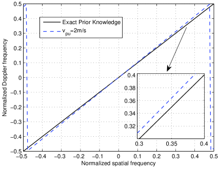
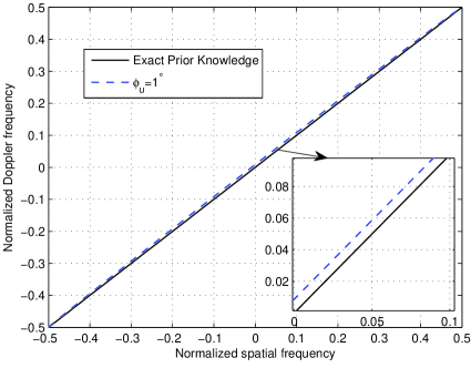
redPrior knowledge uncertainty impact. In the proposed algorithms, the prior knowledge uncertainty, such as velocity misalignment and yaw angle misalignment, will have a great impact on the performance. However, the scheme that employs the CMT will mitigate this impact. To illustrate this, we take a typical airborne radar system for example. The parameters of the radar system are listed at the beginning of Section IV. Consider a far field scenario, the elevation angle will be close to zero resulting in $\cos\theta\approx 1$. Let $v_{pu}$ and $\phi_{u}$ denote the velocity deviation and the yaw angle deviation, respectively. Then, for a discretized azimuth angle $\phi$, the spatial frequency $f_{s}$ and Doppler frequency $f_{d}$ can be represented as

$$f_{s}=\frac{d_{a}}{\lambda_{c}}\sin\phi,$$ (41)

$$f_{d}=\frac{2(v_{p}+v_{pu})T_{r}}{\lambda_{c}}\sin(\phi+\phi_{u}).$$ (42)

From (41) and (42), we see that the prior knowledge uncertainty will affect the position and shape of the clutter ridge, which leads to the mismatch between the exact and the assumed space-time steering vectors. Fig.2 provides a more direct way to illustrate the impact of prior knowledge uncertainty to the clutter ridge in the spatio-temporal plane. By employing a CMT, the clutter spectra will become wider along the clutter ridge in the figure including the exact clutter ridge. From this point of view, the impact of prior knowledge uncertainty is mitigated. Because the methods in [43, 44] and [45] do not consider any strategies to mitigate the impact of prior knowledge uncertainty, the performance will depend highly on the accuracy of the prior knowledge. The KAPE approach in [42] also adopts the CMT and can mitigate the impact of prior knowledge uncertainty in a sense. But the differences between the proposed algorithm and the KAPE approach lie in three aspects. First, the KAPE approach estimates the CCM using the LS or some approximate approaches. While the proposed algorithm estimates the CCM using the Gram-Schmidt orthogonalization procedure (that is not an approximate approach) by exploiting that the clutter subspace is only determined by the space-time steering vectors. Furthermore, for a side-looking ULA radar, the proposed algorithm directly selects a group of linearly independent space-time steering vectors using the LRGP and then takes the Gram-Schmidt orthogonalization procedure to compute the clutter subspace. Second, the proposed algorithm shows evidence bluethat is feasible to directly use the received data vector and the calibrated space-time steering vectors (only the spatial taper without the temporal taper) to compute the parameter ${\boldsymbol{\sigma}}$. Third, the proposed algorithm with an RD version in the following section is presented to further reduce the complexity.

Figure 2: Impact of prior knowledge uncertainty to the clutter ridge in the spatio-temporal plane with (a) velocity deviation $v_{pu}=2$m/s and (b) $\phi_{u}=1^{\circ}$.

III-D Proposed Reduced-Dimension (RD) KA-STAP Algorithms

From the above discussions, one aspect to be noted is that it is impractical to use all the DoFs available at the ULA for reasons of computational complexity when $NM$ is too large. In such situations, a common approach is to break the full DoFs problem into a number of smaller problems via the application of an $MN\times D$ (with $D\ll MN$) transformation matrix ${\bf S}_{D}$ to the data [1]. Our proposed KA-STAP algorithms can be easily extended to this kind of approach. By applying the reduced-dimension transformation matrix ${\bf S}_{D}$ to the data and the space-time steering vectors, we obtain

$$\bar{\bf x}={\bf S}^{H}_{D}{\bf x},\quad\quad\bar{\bf V}={\bf S}^{H}_{D}{\bf V},$$ (43)

where $\bar{}$ denotes the results after the transformation. Then, the reduced-dimension CCM $\bar{\bf R}_{c}$ becomes

$$\bar{\bf R}_{c}={\bf S}^{H}_{D}{\bf R}_{c}{\bf S}_{D}=\bar{\bf V}{\boldsymbol{\Sigma}}\bar{\bf V}=\bar{\bf U}\bar{\boldsymbol{\Gamma}}\bar{\bf U}^{H}.$$ (44)

In a manner similar to that of the proposed full-DoF KA-STAP algorithm described in Section III.B, we compute the orthogonal bases of the clutter subspace ${\bar{\bf U}}$, estimate the CCM $\hat{\bar{\bf R}}_{c}={\bar{\bf U}}\hat{\bar{\boldsymbol{\Gamma}}}{\bar{\bf U}}^{H}$, and then calculate the STAP filter weights according to (27) or (30). When employing a CMT to the ideal clutter covariance matrix, the final RD clutter covariance matrix can be estimated as

$$\hat{\bar{\bf R}}_{c}={red}{\hat{\bar{\bf R}}_{s}\odot\hat{\bar{\bf T}}_{d}=(\hat{\bar{\bf U}}_{s}\hat{\bar{\boldsymbol{\Gamma}}}_{s}\hat{\bar{\bf U}}^{H}_{s})\odot\hat{\bar{\bf T}}_{d},}$$ (45)

redwhere $\hat{\bar{\bf U}}_{s}$ is computed by taking the Gram-Schmidt orthogonalization procedure to $\hat{\bar{\bf V}}_{s}={\bf S}^{H}_{D}\hat{\bf V}_{s}$, $\hat{\bar{\boldsymbol{\Gamma}}}_{s}$ is calculated via (39) using $\bar{\bf x}$ and $\hat{\bar{\bf U}}_{s}$ instead of ${\bf x}$ and $\hat{{\bf U}}_{s}$, and $\hat{\bar{\bf T}}_{d}$ denotes the estimated RD CMT. Again, the STAP filter weights can be computed according to (27) or (30). By inspecting (44) and (45), we find that the computational complexity of our proposed RD-KA-STAP algorithm is related to $D$ instead of $NM$ ($D\ll NM$), which leads to great computation savings.

In this paper, we focus on the reduced-dimension technique known as extended factored (EFA) algorithm or multibin element-space post-Doppler STAP algorithm[1]. The simulations with this technique will show the performance of our proposed RD-KA-STAP algorithm.

III-E Complexity Analysis

Here we illustrate the computational complexity of the proposed algorithms (shortened as LRGP KA-STAP and LRGP RD-KA-STAP) and other existing algorithms, namely, the sample matrix inversion algorithm (SMI), the EFA algorithm in [1], the joint-domain-localized (JDL) algorithm in [7], the CSMIECC algorithm in [43], and the KAPE algorithm in [42]. In Table II, $D$ denotes the size of the reduced dimension. We can see that the computational complexity of our proposed algorithms is significantly lower than the CSMIECC and the KAPE algorithms red($N_{r}\ll N_{c},NM$), which require the pseudo-inverse of the matrix ${\bf V}^{H}{\bf V}$. With regard to the SMI algorithm, our proposed algorithms also show a lower computational complexity because the number of snapshots used for training the filter weights of the SMI is in the order of $2NM$.

TABLE II: Computational Complexity of Algorithms

Algorithm	Estimate the CCM	Compute filter weights
SMI	$O\left(L(NM)^{2}\right)$	$O\left((NM)^{3}\right)$
EFA	$O\left(L(D)^{2}\right)+O\left(L\frac{N}{2}\log_{2}(N)\right)$	$O\left(D^{3}\right)$
JDL	$O\left(L(D)^{2}\right)+O\left(L\frac{NM}{2}\log_{2}(NM)\right)$	$O\left(D^{3}\right)$
CSMIECC	red$O\left(L(NM)^{2}\right)+O\left(N_{c}(NM)^{2}\right)+O\left(N^{3}_{c}+N^{2}_{c}NM\right)$	$O\left((NM)^{3}\right)$
KAPE	red$O\left(N_{c}(NM)^{2}\right)+O\left(N^{3}_{c}+N^{2}_{c}NM\right)$	$O\left((NM)^{3}\right)$
LRGP KA-STAP	red$O\left(\frac{(N_{r}+1)N_{r}NM}{2}+N^{2}_{r}NM\right)+O\left(N_{r}(NM)^{2}\right)$	red$O\left(N_{r}(NM)^{2}\right)$
LRGP RD-KA-STAP	red$O\left(\frac{(N_{r}+1)N_{r}D}{2}+N^{2}_{r}D\right)+O\left(N_{r}D^{2}\right)$	$O\left(D^{3}\right)$

Although the computational complexity of the EFA and JDL algorithms is lower than our proposed LRGP KA-STAP algorithm, two aspects should be noted. One is that the number of snapshots used for training filter weights is much larger than our proposed algorithms. The other is that the computational complexity of EFA and JDL is proportional to the number of Doppler frequencies of interest (we only list the computation complexity for one Doppler frequency). While our proposed algorithms only have to compute the CCM once for different Doppler frequencies of interest. Besides, the computational complexity of our proposed LRGP RD-KA-STAP is lower than the EFA since $L$ in EFA is in the order of $2D$, where $D$ is usually larger than $N_{r}$.

IV Performance Assessment

In this section, we assess the proposed KA-STAP algorithms by computing the output SINR performance and probability of detection performance using simulated radar data. The output SINR is defined by

$${\rm SINR}=\frac{\left|\hat{\bf w}^{H}{\bf s}\right|^{2}}{\left|\hat{\bf w}^{H}{\bf R}\hat{\bf w}\right|}.$$ (46)

redThroughout the simulations, unless otherwise stated, the simulated scenarios use the following parameters: side-looking ULA, uniform transmit pattern, $M=8$, $N=8$, $f_{c}=450$MHz, $f_{r}=300$Hz, $v_{p}=50$m/s, red$d_{a}=\lambda_{c}/2$, $\beta=1$, $N_{r}=\lceil M+\beta(N-1)\rceil=15$, $h_{p}=9000$m, signal-to-noise ratio (SNR) of $0$dB, the target located at $0^{\circ}$ azimuth with Doppler frequency $100$Hz, clutter-to-noise ratio (CNR) of $50$dB, and unitary thermal noise power. All presented results are averaged over $100$ independent Monte Carlo runs.

Figure 3: Impacts of ICM on SINR performance against Doppler frequency with $4$ snapshots and the target Doppler frequency space from $-150$ to $150$Hz. (a): $\sigma_{v}=0$; (b): $\sigma_{v}=0.05$; (c): $\sigma_{v}=0.1$; (d): $\sigma_{v}=0.5$.

IV-A Impact of ICM on the SINR Performance

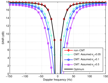
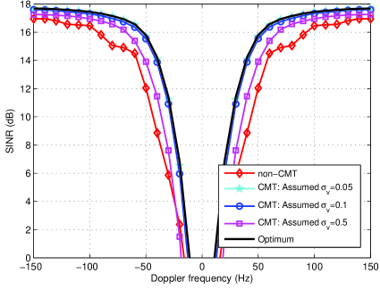
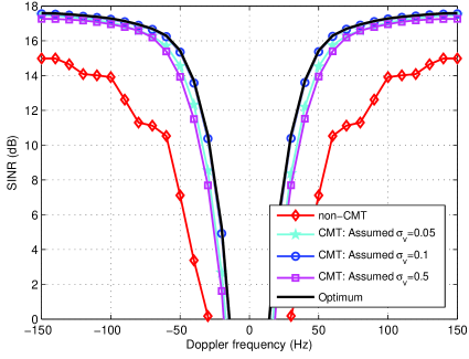
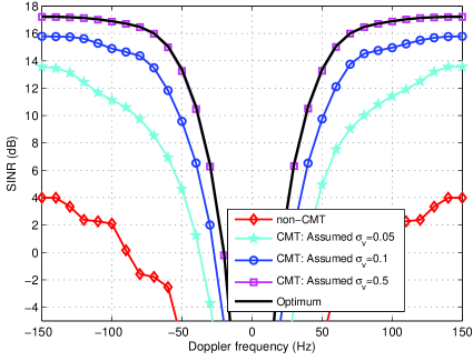
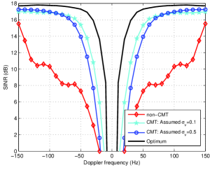
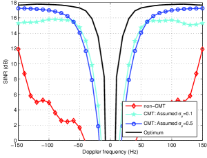
In this subsection, we evaluate the impact on the SINR performance with different ICM for our proposed algorithms. In the examples, we consider four different ICM cases with $\sigma_{v}=0$, $\sigma_{v}=0.05$, $\sigma_{v}=0.1$ and $\sigma_{v}=0.5$. The number of snapshots for training is $4$. In Fig. 3(a), (b), (c) and (d), we show the SINR performance against the target Doppler frequency of our proposed LRGP KA-STAP algorithm both with and without a CMT. From the figures, we observe the following conclusions. (i) When there is non-ICM, the proposed LRGP KA-STAP algorithm without a CMT can obtain the optimum performance since the computed clutter subspace is exact. However, it degrades the SINR performance with the increase of $\sigma_{v}$ resulting in extra sensitivity to the ICM. That is because the computed clutter subspace can not represent the true clutter subspace. (ii) Our proposed LRGP KA-STAP algorithm with a CMT illustrates a robust characteristic to the ICM. When the estimated parameter $\sigma_{v}$ of CMT is correct, we can achieve the optimum SINR performance. Furthermore, it is demonstrated the range of values of CMT mismatch in which the estimated spreading exhibit acceptable SINR performance, which can be useful in applications. This can be interpreted as that the computed clutter subspace via the application of the CMT to the ideal clutter subspace, spans a similar space to the true clutter subspace.

IV-B Impact of Inaccurate Prior Knowledge on the SINR Performance

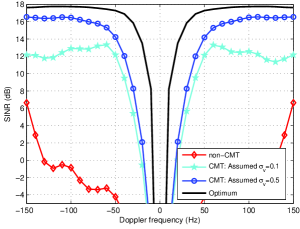
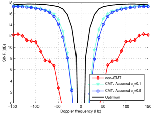
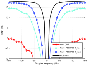
In this subsection, we focus on the impact of inaccurate prior knowledge on the SINR performance of our proposed algorithms. In the first example, we consider the impact of the velocity misalignment by showing the SINR performance against the target Doppler frequency, as shown in Fig.4. Consider three different cases: the velocity misalignments of prior knowledge are (a) $0.5$m/s; (b) $1$m/s; (c) $2$m/s, compared with true platform velocity. The potential Doppler frequency space from $-150$ to $150$Hz is examined and $4$ snapshots are used to train the filter weights. The plots show that the proposed LRGP KA-STAP algorithm without a CMT is sensitive to the velocity misalignment, while the LRGP KA-STAP algorithm with a CMT is robust to that. The reason for this is that the velocity misalignment of prior knowledge will lead to the mismatch between the computed clutter subspace and the true clutter subspace. Although the computed clutter subspace via the CMT can not avoid this situation, it can mitigate this impact. Because the velocity misalignment between the clutter patches and the platform can be seen as the Doppler spreading of the clutter patches. Moreover, the results also show that a slightly larger value of the estimated parameter $\sigma_{v}$ will result in an improved SINR performance for the velocity misalignment case.

The evaluation of the impact caused by the yaw angle misalignment is shown in Fig.5, where we also consider three different cases: the yaw angle misalignments of prior knowledge are (a) $0.2^{\circ}$; (b) $0.5^{\circ}$; (c) $1^{\circ}$. The curves also indicate that: (i) the proposed LRGP KA-STAP algorithm without a CMT is sensitive to the yaw angle misalignment, while the LRGP KA-STAP algorithm with a CMT is robust to that; (ii) a slightly larger value of the estimated parameter $\sigma_{v}$ will result in an improved SINR performance. The misalignment of the yaw angle will lead to a Doppler frequency mismatch between the radar platform and the clutter patches. While the CMT mainly aims at mitigating the performance degradation caused by the clutter Doppler spreading, the CMT will lead to an improved estimated clutter subspace and will exhibit robustness against the yaw angle misalignment.

Figure 4: Impacts of velocity misalignment of the prior knowledge on SINR performance against Doppler frequency with $4$ snapshots and the target Doppler frequency space from $-150$ to $150$Hz. (a): velocity misalignment $0.5$m/s; (b): velocity misalignment $1$m/s; (c): velocity misalignment $2$m/s.

Figure 5: Impacts of yaw angle misalignment of the prior knowledge on SINR performance against Doppler frequency with $4$ snapshots and the target Doppler frequency space from $-150$ to $150$Hz. (a): yaw angle misalignment $0.2^{\circ}$; (b): yaw angle misalignment $0.5^{\circ}$; (c): yaw angle misalignment $1^{\circ}$.

IV-C Comparison With Conventional STAP Algorithms

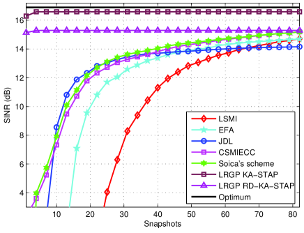
To provide further investigation about the performance of our proposed algorithms, we compare the SINR performance versus the snapshots of our proposed LRGP KA-STAP and LRGP RD-KA-STAP algorithms with the Loaded SMI (LSMI), the EFA algorithm ($3$ Doppler bins), the $3\times 3$ JDL algorithm, redStoica’s scheme in [36] (the prior knowledge covariance matrix is computed in the same way as the CSMIECC bluealgorithm), and the CSMIECC algorithm (the combination parameter is set to $0.6$) in [43], where the simulation results are shown in Fig. 6. Here, we consider a scenario of ICM with $\sigma_{v}=0.5$, and assume the diagonal loading factors for all algorithms are set to the level of the thermal noise power. The parameter $\sigma_{v}$ for our proposed algorithms is redassumed to $1$. The curves in the figure illustrate that our proposed algorithms have a very fast SINR convergence speed which only needs three snapshots for training, and offer significant better SINR steady-state performance compared with the LSMI, EFA, JDL, redStoica’s scheme and CSMIECC algorithms. This is because the proposed algorithms provide a much better estimation of the CCM by using prior knowledge of the data, the low clutter rank property, the geometry of the array and the interference environment. It should be noted that the SINR performance of the LRGP RD-KA-STAP algorithm is worse than that of LRGP KA-STAP with full-DOFs. This is due to the fact that the reduced DOFs will lead to lower computational complexity at the cost of performance degradation.

Figure 6: SINR performance against the number of snapshots considering ICM, where $\sigma_{v}=0.5$.

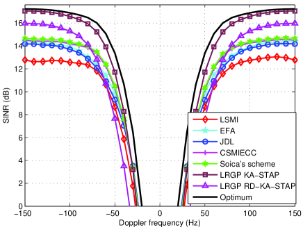
The results in Fig.7 illustrate the SINR performance versus the target Doppler frequency. The number of snapshots used for training in the LSMI, EFA, JDL, redStoica’s scheme and CSMIECC algorithms is set to $48$, while $4$ in our proposed algorithms. It is found that our proposed LRGP KA-STAP algorithm provides the best SINR performance among all algorithms, and forms the narrowest clutter null resulting in improved performance for the detection of slow targets. It is also shown that the performance of the proposed LRGP RD-KA-STAP algorithm is worse than that of LRGP KA-STAP with full-DOFs, but better than other algorithms in most Doppler bins. Note that although the LRGP RD-KA-STAP algorithm performs slightly worse than other algorithms in Doppler range of $-60$ to $60$Hz, it requires much smaller snapshots for training filter weights.

Figure 7: SINR performance versus the target Doppler frequency. The number of snapshots used for training in the LSMI, EFA, JDL and CSMIECC algorithms is set to $48$, while we only use $4$ snapshots for our proposed algorithms.

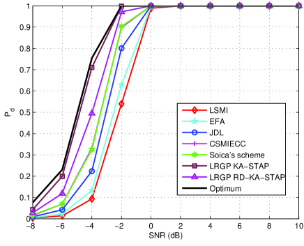
In the next example, as shown in Fig.8, we present the probability of detection performance versus the target SNR for all algorithms. The false alarm rate is set to $10^{-3}$ and for simulation purposes the threshold and probability of detection estimates are based on $10,000$ samples. We suppose the target is injected in the the boresight with Doppler frequency $100$Hz. We note that the proposed algorithms provide suboptimal detection performance using very short snapshots, but remarkably, obtain much higher detection rate than other algorithms at an SNR level from $-8$dB to $0$dB.

Figure 8: Probability of detection performance against the target SNR. Suppose the target is injected in the the boresight with Doppler frequency $100$Hz, and other parameters setting for all algorithms are the same as that in the second example.

V Conclusions

In this paper, novel KA-STAP algorithms have been proposed by using prior knowledge of LRGP to obtain an accurate estimation of the CCM with a very small number of snapshots. By exploiting the fact that the clutter subspace is only determined by the space-time steering vectors, we redhave developed a Gram-Schmidt orthogonalization approach to compute the clutter subspace. In particular, for a side-looking ULA, we have proposed a scheme to directly select a group of linearly independent space-time steering vectors to compute the orthogonal bases of the clutter subspace. Compared with the LSE algorithm, it has not only exhibited a low complexity, but also shown a simple way to compute the CCM. To overcome the performance degradation caused by the non-ideal effects redand the prior knowledge uncertainty, the proposed KA-STAP algorithm that combines the CMT has been presented and a reduced-dimension version has been devised for practical applications. blueThis has also provided evidence that is feasible to directly use the received data vector and the calibrated space-time steering vectors (only the spatial taper without the temporal taper) to compute the assumed clutter amplitude. The simulation results have shown that our proposed algorithms outperform other existing algorithms in terms of SINR steady-state performance, SINR convergence speed and detection performance for a very small number of snapshots, and also exhibit robustness against errors in prior knowledge.

References

- [1] J. Ward, “Space-time adaptive processing for airborne radar,” Technical Report 1015, MIT Lincoln laboratory, Lexington, MAvol, Dec. 1994.
- [2] R. Klemm, Principles of Space-Time Adaptive Processing. Institute of Electical Engineering, London, UK, 2006.
- [3] J. R. Guerci, Space-time adaptive processing for radar. Artech House, 2003.
- [4] W.L. Melvin, “A stap overview,” IEEE A&E Sys. Mag., vol.19, no.1, pp.19-35, 2004.
- [5] A. Haimovich and M. Berin, “Eigenanalysis-based space-time adaptive radar: performance analysis,” IEEE Trans. Aerosp. Electron. Syst., vol.33, no.4, pp.1170-1179, Oct. 1997.
- [6] J. R. Guerci, and J. S. Bergin, “Principal components, covariance matrix tapers, and the subspace leakage problem,” IEEE Trans. Aerosp. Electron. Syst., vol.38, no.1, pp.152-162, Jan. 2002.
- [7] H. Wang and L. Cai, “On adaptive spartial-temporal processingfor airborne surveillance radar systems,” IEEE Trans. Aerosp. Electron. Syst., vol.30, no.3, pp.660-670, 1994.
- [8] J. S. Goldstein and I. S. Reed, ”Theory of partially adaptive radar, ”IEEE Trans. Aerosp. Electron. Syst., vol.33, no.4, pp.1309–1325, Oct. 1997
- [9] J. S. Goldstein, I. S. Reed and P. A. Zulch, “Multistage Partially Adaptive STAP CFAR Detection Algorithm,” IEEE Trans. Aerosp. Electron. Syst., vol.35, no.2, pp.645-661, 1999.
- [10] R. C. de Lamare, M. Haardt and R. Sampaio-Neto, Blind Adaptive Constrained Reduced-Rank Parameter Estimation based on Constant Modulus Design for CDMA Interference Suppression, IEEE Transactions on Signal Processing, vol. 56., no. 6, June 2008.
- [11] P. Clarke, R. C. de Lamare, “Low-Complexity Reduced-Rank Linear Interference Suppression Based on Set-Membership Joint Iterative Optimization for DS-CDMA Systems ”, IEEE Transactions on Vehicular Technology, vol. 60 (9), 4324-4337, 2011.
- [12] N. Song, R. C. de Lamare, M. Haardt, and M. Wolf, Adaptive Widely Linear Reduced-Rank Interference Suppression based on the Multi-Stage Wiener Filter, IEEE Transactions on Signal Processing, vol. 60, no. 8, 2012.
- [13] R. C. de Lamare and Raimundo Sampaio-Neto, “Reduced-rank Interference Suppression for DS-CDMA based on Interpolated FIR Filters”, IEEE Communications Letters, vol. 9, no. 3, March 2005.
- [14] R. C. de Lamare and R. Sampaio-Neto, “Adaptive Reduced-Rank MMSE Filtering with Interpolated FIR Filters and Adaptive Interpolators”, IEEE Signal Processing Letters, vol. 12, no. 3, March, 2005.
- [15] R. C. de Lamare and R. Sampaio-Neto, “Adaptive Interference Suppression for DS-CDMA Systems based on Interpolated FIR Filters with Adaptive Interpolators in Multipath Channels”, IEEE Trans. Vehicular Technology, Vol. 56, no. 6, September 2007.
- [16] R. C. de Lamare and R. Sampaio-Neto, “Adaptive Reduced-Rank MMSE Parameter Estimation based on an Adaptive Diversity Combined Decimation and Interpolation Scheme,” Proc. IEEE International Conference on Acoustics, Speech and Signal Processing, April 15-20, 2007, vol. 3, pp. III-1317-III-1320.
- [17] R. C. de Lamare and R. Sampaio-Neto, “Reduced-Rank Adaptive Filtering Based on Joint Iterative Optimization of Adaptive Filters”, IEEE Signal Processing Letters, Vol. 14, no. 12, December 2007.
- [18] R. C. de Lamare, “Adaptive Reduced-Rank LCMV Beamforming Algorithms Based on Joint Iterative Optimisation of Filters”, Electronics Letters, vol. 44, no. 9, 2008.
- [19] R. C. de Lamare and R. Sampaio-Neto, “Reduced-Rank Space-Time Adaptive Interference Suppression With Joint Iterative Least Squares Algorithms for Spread-Spectrum Systems,” IEEE Transactions on Vehicular Technology, vol.59, no.3, March 2010, pp.1217-1228.
- [20] M. Yukawa, R. C. de Lamare and R Sampaio-Neto, ”Efficient acoustic echo cancellation with reduced-rank adaptive filtering based on selective decimation and adaptive interpolation”, IEEE Transactions on Audio, Speech, and Language Processing, 16 (4), 696-710, 2008.
- [21] R. C. de Lamare and R. Sampaio-Neto, “Adaptive Reduced-Rank Processing Based on Joint and Iterative Interpolation, Decimation, and Filtering,” IEEE Transactions on Signal Processing, vol. 57, no. 7, July 2009, pp. 2503 - 2514.
- [22] L. Wang, R. C. de Lamare, M. Yukawa, “Adaptive Reduced-Rank Constrained Constant Modulus Algorithms Based on Joint Iterative Optimization of Filters for Beamforming,” IEEE Transactions on Signal Processing, , vol. 58, no. 6, June 2010, pp. 2983-2997.
- [23] S. Li, R. C. de Lamare and R. Fa, “Reduced-Rank Linear Interference Supression for DS-UWB Systems Based on Switched Approximations of Adaptive Basis Functions”, IEEE Transactions on Vehicular Technology, vol. 60, no. 2, February 2011.
- [24] R.C. de Lamare and R. Sampaio-Neto, “Adaptive Reduced-Rank Equalization Algorithms Based on Alternating Optimization Design Techniques for MIMO Systems,” IEEE Trans. Vehicular Technology, vol. 60, no. 6, pp.2482-2494, July 2011.
- [25] R.C. de Lamare, R. Sampaio-Neto and M. Haardt, ”Blind Adaptive Constrained Constant-Modulus Reduced-Rank Interference Suppression Algorithms Based on Interpolation and Switched Decimation,” IEEE Trans. on Signal Processing, vol.59, no.2, pp.681-695, Feb. 2011.
- [26] R. C. de Lamare, L. Wang, and R. Fa, “Adaptive reduced-rank LCMV beamforming algorithms based on joint iterative optimization of filters: design and analysis,” Signal Process., vol. 90, pp. 640-652, Feb. 2010.
- [27] R. Fa and R. C. de Lamare, “Reduced-Rank STAP Algorithms using Joint Iterative Optimization of Filters,” IEEE Trans. Aerosp. Electron. Syst., vol.47, no.3, pp.1668-1684, Jul. 2011.
- [28] R. Fa, R. C. de Lamare and L. Wang, “Reduced-rank STAP schemes for airborne radar based on switched joint interpolation, decimation and filtering algorithm,” IEEE Trans. Signal Process., vol.58, no.8, pp.4182-4194, 2010.
- [29] J. R. Roman, M. Rangaswamy, D. W. Davis, Q. Zhang, B. Himed, and J. H. Michels, “Parametric adaptive matched filter for airborne radar applications,” IEEE Trans. Aerosp. Electron. Syst., vol.36, no.2, pp.677-692, 2000.
- [30] Z. Yang, R. C. de Lamare, and X. Li, “-regularized STAP algorithms with a generalized sidelobe canceler architecture for airborne radar”, IEEE Trans. Signal Process., vol. 60, no.2, pp.674-686, 2012.
- [31] Z. Yang, R. C. de Lamare, and X. Li, “Sparsity-aware space-time adaptive processing algorithms with -norm regularisation for airborne radar”, IEt Signal Processing, (5), 413-423, 2012.
- [32] J. R. Guerci and E. J. Baranoski, “Knowledge-Aided adaptive radar at DARPA: an overview,” IEEE Signal Process. Mag., vol.23, no.1, pp.41-50, 2006.
- [33] M. C. Wicks, M. Rangaswamy, R. Adve and T. B. Hale, “Space-time adaptive processing: a knowledge-based perspective for airborne radar,” IEEE Signal Process. Mag., vol.23, no.1, pp.51-65, 2006.
- [34] K. Gerlach and M. L. Picciolo, “Airborne/spacebased radar STAP using a structured covariance matrix,” IEEE Trans. Aerosp. Electron. Syst., vol.39, no.1, pp.269-281, 2003.
- [35] J. S. Bergin, C. M. Teixeira, P. M. Techau and J. R. Guerci, “Improved clutter mitigation performance using knowledge-aided space-time adaptive processing,” IEEE Trans. Aerosp. Electron. Syst., vol.42, no.3, pp.997-1009, 2006.
- [36] P. Stoica, J. Li, X. Zhu and J. R. Guerci, “On using a priori knowledge in space-time adaptive processing,” IEEE Trans. Signal Process., vol.56, no.6, pp.2598-2602, Jun. 2008.
- [37] X. Zhu, J. Li and P. Stoica, “Knowledge-aided space-time adaptive processing,” IEEE Trans. Aerosp. Electron. Syst., vol.47, no.2, pp.1325-1336, Apr. 2011.
- [38] R. Fa, R. C. de Lamare and V. H. Nascimento, “Knowledge-Aided STAP Algorithm Using Convex Combination of Inverse Covariance Matrices for Heterogeneous Clutter”, in Proc. IEEE Int. Conf. Acoust. Speech and Signal Process., pp.2742-2745, Sep. 2010
- [39] S. Bidon, O. Besson and J. Tourneret, “Knowledge-aided STAP in heterogeneous clutter using a hierarchical Bayesian algorithm”, IEEE Trans. Aerosp. Electron. Syst., vol.47, no.3, pp.1863-1879, Jul. 2011
- [40] B. Tang, J. Tang and Y. Peng, “Performance of knowledge aided space time adaptive processing,” IET Radar, Sonar and Navigation, vol.5, no.3, pp.331-340, 2011.
- [41] Y. Wu, J. Tang and Y. Peng, “On the essence of knowledge-aided clutter covariance estimate and its convergence”, IEEE Trans. Aerosp. Electron. Syst., vol.47, no.1, pp.569-585, Jan. 2011
- [42] W. L. Mevin and G. A. Showman, “An approach to knowledge-aided covariance estimation,” IEEE Trans. Aerosp. Electron. Syst., vol.42, no.3, pp.1021-1042, Jul. 2006.
- [43] W. Xie, K. Duan, F. Gao, Y. Wang and Z. Zhang, “Clutter suppression for airborne phased radar with conformal arrays by least squares estimation”, Signal Process., vol.91, no.7, pp.1665-1669, Jul. 2011
- [44] I. W. Selesnick, S. U. Pillai, K. Y. Li and B. Himed, “Angle-Doppler processing using sparse regularization”, in Proc. IEEE Int. Conf. Acoust. Speech and Signal Process., pp.2750-2753, 2010.
- [45] C. Chen, and P. P. Vaidyanathan, “MIMO radar space-time adaptive processing using prolate spheroidal wave functions”, IEEE Trans. Signal Process., vol.56, no.2, pp.623-635, Feb. 2008.
- [46] Q. Zhang, and W. B. Mikhael, “Estimation of the clutter rank in the case of subarraying for space-time adaptive processing”, Electronics Letters, vol.33 no.5, pp.419-420, Feb. 1997.
- [47] N. A. Goodman, and J. M. Stiles, “On clutter rank observed by arbitrary arrays”, IEEE Trans. Signal Process., vol.55, no.1, pp.178-186, Jan. 2007.
- [48] G. Xu, and T. Kailath, “Fast subspace decomposition”, IEEE Trans. Signal Process., vol.42, no.3, pp.539-551, Mar. 1994
- [49] R. A. Horn and C. R. Johnson, Matrix Analysis. Cambridge, U.K.: Cambridge Univ. Press, 1985.