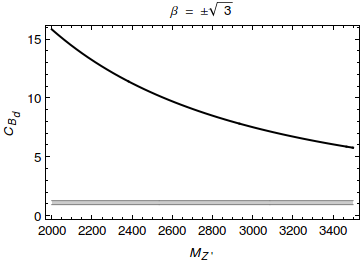
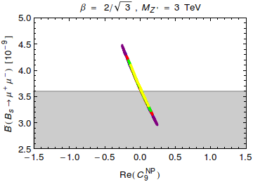
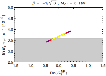
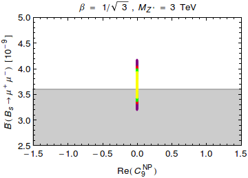
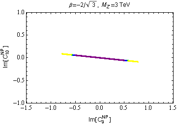
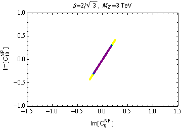
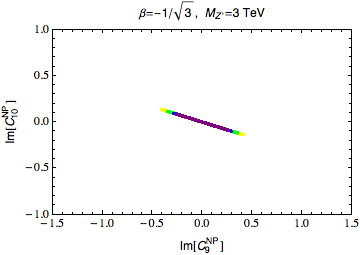
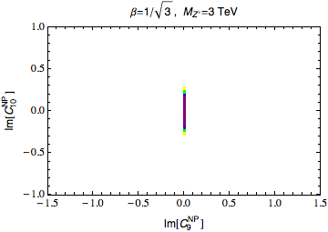
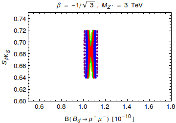
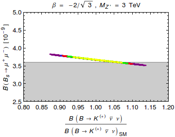
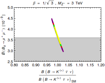
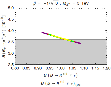
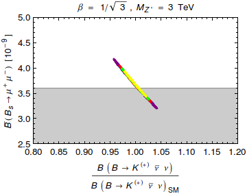
FLAVOUR(267104)-ERC-55

BARI-TH/13-681

331 models facing new bsμ+μbold-→𝑏𝑠superscript𝜇superscript𝜇b\to s\mu^{+}\mu^{-} data
Andrzej J. Burasa,b, Fulvia De Fazioc and Jennifer Girrbacha,b
aTUM Institute for Advanced Study, Lichtenbergstr. 2a, D-85747 Garching, Germany
bPhysik Department, Technische Universität München, James-Franck-Straße,
D-85747 Garching, Germany
cIstituto Nazionale di Fisica Nucleare, Sezione di Bari, Via Orabona 4, I-70126 Bari, Italy


Abstract

We investigate how the 331 models, based on the gauge group SU(3)C×SU(3)L×U(1)X𝑆𝑈subscript3𝐶𝑆𝑈subscript3𝐿𝑈subscript1𝑋SU(3)_{C}\times SU(3)_{L}\times U(1)_{X} face new data on Bs,dμ+μsubscript𝐵𝑠𝑑superscript𝜇superscript𝜇B_{s,d}\to\mu^{+}\mu^{-} and BdK(K)μ+μsubscript𝐵𝑑superscript𝐾𝐾superscript𝜇superscript𝜇B_{d}\to K^{*}(K)\mu^{+}\mu^{-} taking into account present constraints from ΔF=2Δ𝐹2\Delta F=2 observables, low energy precision measurements, LEP-II and the LHC data. In these models new sources of flavour and CP violation originate dominantly through flavour violating interactions of ordinary quarks and leptons with a new heavy Zsuperscript𝑍Z^{\prime} gauge boson. The strength of the relevant couplings is governed by four new parameters in the quark sector and the parameter β𝛽\beta which in these models determines the charges of new heavy fermions and gauge bosons. We study the implications of these models for β=±n/3𝛽plus-or-minus𝑛3\beta=\pm n/\sqrt{3} with n=1,2,3𝑛123n=1,2,3. The case β=3𝛽3\beta=-\sqrt{3} leading to Landau singularities for MZ4TeVsubscript𝑀superscript𝑍4TeVM_{Z^{\prime}}\approx 4\,{\rm TeV} can be ruled out when the present constraints on Zsuperscript𝑍Z^{\prime} couplings, in particular from LEP-II, are taken into account. For n=1,2𝑛12n=1,2 interesting results are found for MZ<4TeVsubscript𝑀superscript𝑍4TeVM_{Z^{\prime}}<4\,{\rm TeV} with largest NP effects for β<0𝛽0\beta<0 in BdKμ+μsubscript𝐵𝑑superscript𝐾superscript𝜇superscript𝜇B_{d}\to K^{*}\mu^{+}\mu^{-} and the ones in Bs,dμ+μsubscript𝐵𝑠𝑑superscript𝜇superscript𝜇B_{s,d}\to\mu^{+}\mu^{-} for β>0𝛽0\beta>0. As Re(C9NP)ResuperscriptsubscriptC9NP\rm{Re}(C_{9}^{\rm NP}) can reach the values 0.80.8-0.8 and 0.40.4-0.4 for n=2𝑛2n=2 and n=1𝑛1n=1, respectively the BdKμ+μsubscript𝐵𝑑superscript𝐾superscript𝜇superscript𝜇B_{d}\to K^{*}\mu^{+}\mu^{-} anomalies can be softened with the size depending on ΔMs/(ΔMs)SMΔsubscript𝑀𝑠subscriptΔsubscript𝑀𝑠SM\Delta M_{s}/(\Delta M_{s})_{\rm SM} and the CP-asymmetry Sψϕsubscript𝑆𝜓italic-ϕS_{\psi\phi}. A correlation between Re(C9NP)ResubscriptsuperscriptCNP9\rm{Re}(C^{\rm NP}_{9}) and ¯(Bsμ+μ)¯subscript𝐵𝑠superscript𝜇superscript𝜇\overline{\mathcal{B}}(B_{s}\to\mu^{+}\mu^{-}), identified for β<0𝛽0\beta<0, implies for negative Re(C9NP)ResubscriptsuperscriptCNP9\rm{Re}(C^{\rm NP}_{9}) uniquely suppression of ¯(Bsμ+μ)¯subscript𝐵𝑠superscript𝜇superscript𝜇\overline{\mathcal{B}}(B_{s}\to\mu^{+}\mu^{-}) relative to its SM value which is favoured by the data. In turn also Sψϕ<SψϕSMsubscript𝑆𝜓italic-ϕsuperscriptsubscript𝑆𝜓italic-ϕSMS_{\psi\phi}<S_{\psi\phi}^{\rm SM} is favoured with Sψϕsubscript𝑆𝜓italic-ϕS_{\psi\phi} having dominantly opposite sign to SψϕSMsuperscriptsubscript𝑆𝜓italic-ϕSMS_{\psi\phi}^{\rm SM} and closer to its central experimental value. Another triple correlation is the one between Re(C9NP)ResubscriptsuperscriptCNP9\rm{Re}(C^{\rm NP}_{9}), ¯(Bsμ+μ)¯subscript𝐵𝑠superscript𝜇superscript𝜇\overline{\mathcal{B}}(B_{s}\to\mu^{+}\mu^{-}) and (BdKμ+μ)subscript𝐵𝑑𝐾superscript𝜇superscript𝜇\mathcal{B}(B_{d}\to K\mu^{+}\mu^{-}). NP effects in bsνν¯𝑏𝑠𝜈¯𝜈b\to s\nu\bar{\nu} transitions, K+π+νν¯superscript𝐾superscript𝜋𝜈¯𝜈K^{+}\rightarrow\pi^{+}\nu\bar{\nu} and KLπ0νν¯subscript𝐾𝐿superscript𝜋0𝜈¯𝜈K_{L}\rightarrow\pi^{0}\nu\bar{\nu} turn out to be small. We find that the absence of BdKμ+μsubscript𝐵𝑑superscript𝐾superscript𝜇superscript𝜇B_{d}\to K^{*}\mu^{+}\mu^{-} anomalies in the future data and confirmation of the suppression of ¯(Bsμ+μ)¯subscript𝐵𝑠superscript𝜇superscript𝜇\overline{\mathcal{B}}(B_{s}\to\mu^{+}\mu^{-}) relative to its SM value would favour β=1/3𝛽13\beta=1/\sqrt{3} and MZ3TeVsubscript𝑀superscript𝑍3TeVM_{Z^{\prime}}\approx 3\,{\rm TeV}. Assuming lepton universality, we find an upper bound |C9NP|1.1(1.4)subscriptsuperscript𝐶NP91.11.4|C^{\rm NP}_{9}|\leq 1.1(1.4) from LEP-II data for all Zsuperscript𝑍Z^{\prime} models with only left-handed flavour violating couplings to quarks when NP contributions to ΔMsΔsubscript𝑀𝑠\Delta M_{s} at the level of 10%(15%)percent10percent1510\%(15\%) are allowed.

1 Introduction

The great expectations to find New Physics (NP) at the LHC did not materialize until now. In particular the order of magnitude enhancements of the branching ratio for Bsμ+μsubscript𝐵𝑠superscript𝜇superscript𝜇B_{s}\to\mu^{+}\mu^{-} decay over its Standard Model (SM) value, possible in supersymmetric models and models with tree-level heavy neutral scalar and pseudoscalar exchanges, are presently ruled out. This is also the case of 𝒪(1)𝒪1\mathcal{O}(1) values of the CP-asymmetry Sψϕsubscript𝑆𝜓italic-ϕS_{\psi\phi} which could also be accommodated in these models. A recent review can be found in [1].

While for the models in question these new flavour data are a big disappointment, for other models like the ones with constrained minimal flavour violation (CMFV), 331331331 models [2] and Littlest Higgs Model with T-parity [3] they brought a relief as in these models NP effects were naturally predicted to be small. On the other hand the most recent data from LHCb and CMS bring new challenges for the latter models:

  • The LHCb and CMS collaborations presented new results on Bs,dμ+μsubscript𝐵𝑠𝑑superscript𝜇superscript𝜇B_{s,d}\to\mu^{+}\mu^{-} [4, 5, 6]. While the branching ratio for Bsμ+μsubscript𝐵𝑠superscript𝜇superscript𝜇B_{s}\to\mu^{+}\mu^{-} as stated above turns out to be rather close to the SM prediction, although a bit lower than the latter, the central value for the one of Bdμ+μsubscript𝐵𝑑superscript𝜇superscript𝜇B_{d}\to\mu^{+}\mu^{-} is by a factor of 3.5 higher than its SM value.

  • LHCb collaboration reported new results on angular observables in BdKμ+μsubscript𝐵𝑑superscript𝐾superscript𝜇superscript𝜇B_{d}\to K^{*}\mu^{+}\mu^{-} that show departures from SM expectations [7, 8]. Moreover, new data on the observable FLsubscript𝐹𝐿F_{L}, consistent with LHCb value in [7] have been presented by CMS [9].

In particular the anomalies in BdKμ+μsubscript𝐵𝑑superscript𝐾superscript𝜇superscript𝜇B_{d}\to K^{*}\mu^{+}\mu^{-} triggered two sophisticated analyses [10, 11] with the goal to understand the data and to indicate what type of NP could be responsible for these departures from the SM. Subsequently several other analyses of these data have been presented in [12, 13, 14, 15, 16, 17] and very recently in [18].

The outcome of these efforts can be summarized briefly as follows. There seems to be a consensus among different groups that NP definitely affects the Wilson coefficient C9subscript𝐶9C_{9} [10, 11, 13, 17, 18] with the value of the shift in C9subscript𝐶9C_{9} depending on the analysis considered:

1.9C9NP0.5.1.9subscriptsuperscript𝐶NP90.5-1.9\leq C^{\rm NP}_{9}\leq-0.5. (1)

There is also a consensus that small negative NP contributions to the the Wilson coefficient C7γsubscript𝐶7𝛾C_{7\gamma} could together with C9NPsubscriptsuperscript𝐶NP9C^{\rm NP}_{9} provide the explanation of the data [10, 11]. On the other hand as seen in the analyses in [11, 13, 17], a particularly successful scenario is the one with participation of right-handed currents

C9NP<0,C9>0,C9C9NP.formulae-sequencesubscriptsuperscript𝐶NP90formulae-sequencesubscriptsuperscript𝐶90subscriptsuperscript𝐶9subscriptsuperscript𝐶NP9C^{\rm NP}_{9}<0,\qquad C^{\prime}_{9}>0,\qquad C^{\prime}_{9}\approx-C^{\rm NP}_{9}. (2)

However a very recent analysis in [18] challenges this solution favouring the one with NP contributions dominantly represented by C9NP1.5subscriptsuperscript𝐶NP91.5C^{\rm NP}_{9}\approx-1.5 with much smaller NP contributions to the remaining Wilson coefficients, in particular C9subscriptsuperscript𝐶9C^{\prime}_{9}.

For the models presented here sorting out these differences is important as in these models C9=0subscriptsuperscript𝐶90C^{\prime}_{9}=0 and as demonstrated in [2, 19] NP contributions to C7γsubscript𝐶7𝛾C_{7\gamma} are totally negligible. Thus C9NPsubscriptsuperscript𝐶NP9C^{\rm NP}_{9} remains the only coefficient which could help in explaining the BdKμ+μsubscript𝐵𝑑superscript𝐾superscript𝜇superscript𝜇B_{d}\to K^{*}\mu^{+}\mu^{-} anomalies. In our view this is certainly not excluded [10, 12, 13, 14, 15, 18], in particular if these anomalies would soften with time. It should be emphasized at this point that these analyses are subject to theoretical uncertainties, which have been discussed at length in [20, 21, 22, 23, 10, 24] and it remains to be seen whether the observed anomalies are only result of statistical fluctuations and/or underestimated error uncertainties.

Assuming that indeed NP is at work here, one of the physical mechanisms behind these deviations that seems to emerge from these studies is the presence of tree-level Zsuperscript𝑍Z^{\prime} exchanges. In [19] we have presented an anatomy of Zsuperscript𝑍Z^{\prime} contributions to flavour changing neutral current processes (FCNC) identifying various correlations between various observables characteristic for this NP scenario. Recently we have analyzed how this scenario faces the new data listed above [13] including the correlation with the values of CBq=ΔMq/(ΔMq)SMsubscript𝐶subscript𝐵𝑞Δsubscript𝑀𝑞subscriptΔsubscript𝑀𝑞SMC_{B_{q}}=\Delta M_{q}/(\Delta M_{q})_{\rm SM}, Sψϕsubscript𝑆𝜓italic-ϕS_{\psi\phi} and SψKSsubscript𝑆𝜓subscript𝐾𝑆S_{\psi K_{S}} which should be precisely determined in this decade.

The dominant role in [13] was played by the so-called LHS scenario in which the flavour violating couplings of Zsuperscript𝑍Z^{\prime} to quarks were purely left-handed. While, in agreement with [11] and recently with [17] it has been found that the presence of right-handed couplings leading to a non-vanishing C9superscriptsubscript𝐶9C_{9}^{\prime} gives a better description of the data than the LHS scenario, it is clear that in view of theoretical and experimental uncertainties the LHS scenario remains as a viable alternative.

The nice virtue of the LHS scenario is that for certain choices of the Zsuperscript𝑍Z^{\prime} couplings the model resembles the structure of CMFV or models with U(2)3𝑈superscript23U(2)^{3} flavour symmetry. Moreover as no new operators beyond those present in the SM are present, the non-perturbative uncertainties are the same as in the SM, still allowing for non-MFV contributions beyond those present in U(2)3𝑈superscript23U(2)^{3} models. In particular the stringent CMFV relation between ΔMs,dΔsubscript𝑀𝑠𝑑\Delta M_{s,d} and (Bs,dμ+μ)subscript𝐵𝑠𝑑superscript𝜇superscript𝜇\mathcal{B}(B_{s,d}\to\mu^{+}\mu^{-}) [25] valid in the simplest U(2)3𝑈superscript23U(2)^{3} models is violated in the LHS scenario as analyzed in detail in [13]. Another virtue of the LHS scenario is the paucity of its parameters that enter all flavour observables in a given meson system which should be contrasted with most NP scenarios outside the MFV framework. Indeed, if we concentrate on Bs0B¯s0superscriptsubscript𝐵𝑠0superscriptsubscript¯𝐵𝑠0B_{s}^{0}-\bar{B}_{s}^{0} mixing, bsμ+μ𝑏𝑠superscript𝜇superscript𝜇b\to s\mu^{+}\mu^{-} and bsνν¯𝑏𝑠𝜈¯𝜈b\to s\nu\bar{\nu} observables, for a given mass MZsubscript𝑀superscript𝑍M_{Z^{\prime}} there are only four new parameters to our disposal: the three couplings (our normalizations of couplings are given in Section 2)

ΔLsb(Z),ΔAμμ¯(Z),ΔVμμ¯(Z),superscriptsubscriptΔ𝐿𝑠𝑏superscript𝑍superscriptsubscriptΔ𝐴𝜇¯𝜇superscript𝑍superscriptsubscriptΔ𝑉𝜇¯𝜇superscript𝑍\Delta_{L}^{sb}(Z^{\prime}),\quad\Delta_{A}^{\mu\bar{\mu}}(Z^{\prime}),\quad\Delta_{V}^{\mu\bar{\mu}}(Z^{\prime}), (3)

of which the first one is generally complex and the other two real. The couplings ΔA,Vμμ¯(Z)superscriptsubscriptΔ𝐴𝑉𝜇¯𝜇superscript𝑍\Delta_{A,V}^{\mu\bar{\mu}}(Z^{\prime}) are defined in (19) and due to SU(2)L𝑆𝑈subscript2𝐿SU(2)_{L} symmetry implying in LHS ΔLνν¯(Z)=ΔLμμ¯(Z)superscriptsubscriptΔ𝐿𝜈¯𝜈superscript𝑍superscriptsubscriptΔ𝐿𝜇¯𝜇superscript𝑍\Delta_{L}^{\nu\bar{\nu}}(Z^{\prime})=\Delta_{L}^{\mu\bar{\mu}}(Z^{\prime}) one also has

ΔLνν¯(Z)=ΔVμμ¯(Z)ΔAμμ¯(Z)2.superscriptsubscriptΔ𝐿𝜈¯𝜈superscript𝑍superscriptsubscriptΔ𝑉𝜇¯𝜇superscript𝑍superscriptsubscriptΔ𝐴𝜇¯𝜇superscript𝑍2\Delta_{L}^{\nu\bar{\nu}}(Z^{\prime})=\frac{\Delta_{V}^{\mu\bar{\mu}}(Z^{\prime})-\Delta_{A}^{\mu\bar{\mu}}(Z^{\prime})}{2}. (4)

Extending these considerations to Bdsubscript𝐵𝑑B_{d} and K𝐾K meson systems brings in four additional parameters, the complex couplings:

ΔLdb(Z),ΔLsd(Z).superscriptsubscriptΔ𝐿𝑑𝑏superscript𝑍superscriptsubscriptΔ𝐿𝑠𝑑superscript𝑍\Delta_{L}^{db}(Z^{\prime}),\qquad\Delta_{L}^{sd}(Z^{\prime}). (5)

Thus in this general LHS scenario we deal with eight new parameters. Further reduction of parameters is only possible in a concrete dynamical model. In this context an interesting class of dynamical models representing LHS scenario are the 331 models based on the gauge group SU(3)C×SU(3)L×U(1)X𝑆𝑈subscript3𝐶𝑆𝑈subscript3𝐿𝑈subscript1𝑋SU(3)_{C}\times SU(3)_{L}\times U(1)_{X} [26, 27]. A detailed analysis of FCNC processes in one of these models has been presented by us in [2]. Selection of earlier analyses of various aspects of these models related to our paper can be found in [28, 29, 30, 31, 32, 33, 34, 35, 36, 37].

The nice feature of these models is a small number of free parameters which is lower than present in the general LHS scenario considered in [19, 13]. This allows to find certain correlations between different meson systems which is not possible in the general case. Indeed the strength of the relevant Zsuperscript𝑍Z^{\prime} couplings to down-quarks is governed by two mixing parameters, two CP-violating phases and the parameter β𝛽\beta which defines111 Up to the choice of the representation of the gauge group according to which the fermions should transform, as will be better clarified in the next section. a given 331 model and determines the charges of new heavy fermions and gauge bosons. Thus for a given MZsubscript𝑀superscript𝑍M_{Z^{\prime}} and β𝛽\beta there are only four free parameters to our disposal. In particular for a given β𝛽\beta, the couplings of Zsuperscript𝑍Z^{\prime} to leptons are fixed. As evident from the general analysis of LHS scenario in [13], knowing the latter couplings simplifies the analysis significantly, increasing simultaneously the predictive power of the theory.

In [2] the relevant couplings have been presented for arbitrary β𝛽\beta but the detailed FCNC analysis has been only performed for β=1/3𝛽13\beta=1/\sqrt{3}. While this model provides interesting results for Bs,dμ+μsubscript𝐵𝑠𝑑superscript𝜇superscript𝜇B_{s,d}\to\mu^{+}\mu^{-}, it fails in the case of anomalies in BdKμ+μsubscript𝐵𝑑superscript𝐾superscript𝜇superscript𝜇B_{d}\to K^{*}\mu^{+}\mu^{-} because in this model the coupling ΔVμμ¯(Z)superscriptsubscriptΔ𝑉𝜇¯𝜇superscript𝑍\Delta_{V}^{\mu\bar{\mu}}(Z^{\prime}) and consequently the Wilson coefficient C9NPsubscriptsuperscript𝐶NP9C^{\rm NP}_{9} turn out to be very small.

It has been pointed out recently in [14] that for β=3𝛽3\beta=-\sqrt{3} a very different picture arises. Indeed in this case ΔVμμ¯(Z)superscriptsubscriptΔ𝑉𝜇¯𝜇superscript𝑍\Delta_{V}^{\mu\bar{\mu}}(Z^{\prime}) is much larger than for β=1/3𝛽13\beta=1/\sqrt{3} so that the BdKμ+μsubscript𝐵𝑑superscript𝐾superscript𝜇superscript𝜇B_{d}\to K^{*}\mu^{+}\mu^{-} anomaly can be in principle successfully addressed. Simultaneously the coupling ΔAμμ¯(Z)superscriptsubscriptΔ𝐴𝜇¯𝜇superscript𝑍\Delta_{A}^{\mu\bar{\mu}}(Z^{\prime}) turns out to be small so that NP contributions to Bsμ+μsubscript𝐵𝑠superscript𝜇superscript𝜇B_{s}\to\mu^{+}\mu^{-} are small in agreement with the data. Moreover aligning the new mixing matrix VLsubscript𝑉𝐿V_{L} with the CKM matrix, the authors end up with a very simple model in which the only new parameter relevant for their analysis is MZsubscript𝑀superscript𝑍M_{Z^{\prime}} and the negative sign of C9NPsubscriptsuperscript𝐶NP9C^{\rm NP}_{9} required by the BdKμ+μsubscript𝐵𝑑superscript𝐾superscript𝜇superscript𝜇B_{d}\to K^{*}\mu^{+}\mu^{-} anomaly is uniquely predicted.

Unfortunately this model has several problems, in particular in the MFV limit considered in [14], which in our view eliminates it as a valid description of the present flavour data. As discussed in Appendix C these problems originate in the known fact that the 331 models with β=±3𝛽plus-or-minus3\beta=\pm\sqrt{3} imply a Landau singularity for sin2θW=0.25superscript2subscript𝜃𝑊0.25\sin^{2}\theta_{W}=0.25 and this value is reached through the renormalization group evolution of the SM couplings for MZsubscript𝑀superscript𝑍M_{Z^{\prime}} typically around 4TeV4TeV4\,{\rm TeV}, scales not much higher than the present lower bounds on MZsubscript𝑀superscript𝑍M_{Z^{\prime}}.

Yet, the observation of the authors of [14] that negative values of β𝛽\beta could provide solution to BdKμ+μsubscript𝐵𝑑superscript𝐾superscript𝜇superscript𝜇B_{d}\to K^{*}\mu^{+}\mu^{-} anomalies motivates us to generalize our phenomenological analysis of 331 model in [2] from β=1/3𝛽13\beta=1/\sqrt{3} to arbitrary values of β𝛽\beta, both positive and negative, for which the Landau singularity in question is avoided up to the very high scales, even as high as GUTs scales. This generalization is in fact straight forward as in [2] we have provided formulae for the Zsuperscript𝑍Z^{\prime} couplings to quarks and leptons for arbitrary β𝛽\beta222 See also [31]. and the expressions for various flavour observables as functions of β𝛽\beta can be directly obtained from the formulae of that paper. In this context we will concentrate our analysis on the cases β=±n/3𝛽plus-or-minus𝑛3\beta=\pm n/\sqrt{3} with n=1,2𝑛12n=1,2 choosing MZ=3TeVsubscript𝑀superscript𝑍3TeVM_{Z^{\prime}}=3\,{\rm TeV} in order to satisfy existing bounds from flavour conserving observables. A simple scaling law allows then to obtain predictions for other values of MZsubscript𝑀superscript𝑍M_{Z^{\prime}}.

However, in contrast to our numerical analysis in [2] which assumed certain fixed values of B^BsFBssubscript^𝐵subscript𝐵𝑠subscript𝐹subscript𝐵𝑠\sqrt{\hat{B}_{B_{s}}}F_{B_{s}} and B^BdFBdsubscript^𝐵subscript𝐵𝑑subscript𝐹subscript𝐵𝑑\sqrt{\hat{B}_{B_{d}}}F_{B_{d}} we will investigate in the spirit of our recent paper [13] how our results depend on

CBq=ΔMq(ΔMq)SM,Sψϕ,SψKSsubscript𝐶subscript𝐵𝑞Δsubscript𝑀𝑞subscriptΔsubscript𝑀𝑞SMsubscript𝑆𝜓italic-ϕsubscript𝑆𝜓subscript𝐾𝑆C_{B_{q}}=\frac{\Delta M_{q}}{(\Delta M_{q})_{\rm SM}},\qquad S_{\psi\phi},\qquad S_{\psi K_{S}} (6)

which should be precisely determined in this decade.

Our paper is organized as follows. In Section 2 we review very briefly the basic aspects of 331 models, recalling their free parameters and the general formulae for the couplings of Zsuperscript𝑍Z^{\prime} to quarks and leptons for arbitrary β𝛽\beta. We also present a table with the values of flavour diagonal couplings of Zsuperscript𝑍Z^{\prime} to quarks and leptons for n=1,2,3𝑛123n=1,2,3 which should facilitate other researchers to test precisely these models in processes not considered by us. In Section 3 we collect formulae for various Wilson coefficients and one-loop master functions in terms of the couplings of Section 2. This will allow us to identify certain properties and correlations between various observables that will be explicitly seen in our numerical analysis. As all relevant formulae for various branching ratios and other observables have been presented in [2] we recall in Section 4 only crucial observables and their status in the SM and experiment. The strategy for our analysis is presented in Section 5 and its execution in Section 6. In Section 7 we present predictions for low energy precision observables which could provide additional tests of the models considered and analyse also the bounds from LEP-II. We also comment on the bounds on MZsubscript𝑀superscript𝑍M_{Z^{\prime}} from the LHC. We summarize the main results of our paper in Section 8. Some useful information can also be found in three appendices.

2 The 331 models and their couplings

2.1 The 331 models

The name 331 encompasses a class of models based on the gauge group SU(3)C×SU(3)L×U(1)X𝑆𝑈subscript3𝐶𝑆𝑈subscript3𝐿𝑈subscript1𝑋SU(3)_{C}\times SU(3)_{L}\times U(1)_{X} [26, 27], that is at first spontaneously broken to the SM group SU(3)C×SU(2)L×U(1)Y𝑆𝑈subscript3𝐶𝑆𝑈subscript2𝐿𝑈subscript1𝑌SU(3)_{C}\times SU(2)_{L}\times U(1)_{Y} and then undergoes the spontaneous symmetry breaking to SU(3)C×U(1)Q𝑆𝑈subscript3𝐶𝑈subscript1𝑄SU(3)_{C}\times U(1)_{Q}. The extension of the gauge group with respect to SM leads to interesting consequences. The first one is that the requirement of anomaly cancellation together with that of asymptotic freedom of QCD implies that the number of generations must necessarily be equal to the number of colours, hence giving an explanation for the existence of three generations. Furthermore, quark generations should transform differently under the action of SU(3)L𝑆𝑈subscript3𝐿SU(3)_{L}. In particular, two quark generations should transform as triplets, one as an antitriplet. Choosing the latter to be the third generation, this different treatment could be at the origin of the large top quark mass. This choice imposes that the leptons should transform as antitriplets. However, one could choose a different scenario in which the role of triplets and antitriplets is exchanged, provided that the number of triplets equals that of antitriplets, in order to fulfil the anomaly cancellation requirement. Therefore, different versions of the model are obtained according to the way one fixes the fermion representations. The fermion representations for specific 331 models analyzed in our paper are described in detail in [2].

A fundamental relation holds among some of the generators of the group:

Q=T3+βT8+X,𝑄subscript𝑇3𝛽subscript𝑇8𝑋Q=T_{3}+\beta T_{8}+X, (7)

where Q𝑄Q indicates the electric charge, T3subscript𝑇3T_{3} and T8subscript𝑇8T_{8} are two of the SU(3)𝑆𝑈3SU(3) generators and X𝑋X is the generator of U(1)X𝑈subscript1𝑋U(1)_{X}. β𝛽\beta is a key parameter that defines a specific variant of the model. The 331 models comprise several new particles. There are new gauge bosons Y𝑌Y and V𝑉V and new heavy fermions, all with electric charges depending on β𝛽\beta. Also the Higgs system is extended.

As analyzed in detail in [31] and stated in that paper β𝛽\beta can be arbitrary. Yet due to the fact that in 331 models

MZ2=g2u2cW23[1(1+β2)sW2]subscriptsuperscript𝑀2superscript𝑍superscript𝑔2superscript𝑢2superscriptsubscript𝑐𝑊23delimited-[]11superscript𝛽2superscriptsubscript𝑠𝑊2M^{2}_{Z^{\prime}}=\frac{g^{2}u^{2}c_{W}^{2}}{3[1-(1+\beta^{2})s_{W}^{2}]}\,\, (8)

where u𝑢u is the vacuum expectation value related to the first symmetry breaking it is evident that only values of β𝛽\beta satisfying

[1(1+β2)sW2]>0delimited-[]11superscript𝛽2superscriptsubscript𝑠𝑊20[1-(1+\beta^{2})s_{W}^{2}]>0 (9)

are allowed. With the known value of sW2superscriptsubscript𝑠𝑊2s_{W}^{2} this means that

|β|3𝛽3|\beta|\leq\sqrt{3} (10)

and in fact the only explicit models analyzed in the literature are the ones with β=±1/3𝛽plus-or-minus13\beta=\pm 1/\sqrt{3} and β=±3𝛽plus-or-minus3\beta=\pm\sqrt{3}. But only for β=±1/3𝛽plus-or-minus13\beta=\pm 1/\sqrt{3} one can avoid the presence of exotic charges both in the fermion and gauge boson sectors. If one considers only

β=±n3,n=1,2,3formulae-sequence𝛽plus-or-minus𝑛3𝑛123\beta=\pm\frac{n}{\sqrt{3}},\qquad n=1,2,3 (11)

then for n=1𝑛1n=1 there are singly charged Y±superscript𝑌plus-or-minusY^{\pm} bosons and neutral ones V0(V¯0)superscript𝑉0superscript¯𝑉0V^{0}(\bar{V}^{0}), while for n=3𝑛3n=3 one finds instead two new singly charged bosons V±superscript𝑉plus-or-minusV^{\pm} and two doubly charged ones Y±±superscript𝑌plus-or-minusabsentplus-or-minusY^{\pm\pm}. For n=2𝑛2n=2 exotic charges ±1/2plus-or-minus12\pm 1/2 and ±3/2plus-or-minus32\pm 3/2 for gauge bosons are found. From Table 1 in [2] we also find that while for n=1𝑛1n=1 no exotic charges for heavy fermions are present, for n=2𝑛2n=2 heavy quarks carry exotic electric charges ±5/6plus-or-minus56\pm 5/6 and ±7/6plus-or-minus76\pm 7/6 while heavy leptons ±1/2plus-or-minus12\pm 1/2 and ±3/2plus-or-minus32\pm 3/2. Discovering such fermions at the LHC would be a spectacular event. We refer to [2] for further details. In principle β𝛽\beta could be a continuous variable satisfying (10) but in the present paper we will only consider the cases n=1,2,3𝑛123n=1,2,3.

Most importantly for our paper for all β𝛽\beta a new neutral gauge boson Zsuperscript𝑍Z^{\prime} is present. This represents a very appealing feature, since Zsuperscript𝑍Z^{\prime} mediates tree level flavour changing neutral currents (FCNC) in the quark sector and could be responsible for the recent anomalies as indicated by their recent extensive analyses.

As in the SM, quark mass eigenstates are defined upon rotation of flavour eigenstates through two unitary matrices ULsubscript𝑈𝐿U_{L} (for up-type quarks) and VLsubscript𝑉𝐿V_{L} (for down-type quarks). The relation

VCKM=ULVLsubscript𝑉CKMsuperscriptsubscript𝑈𝐿subscript𝑉𝐿V_{\rm CKM}=U_{L}^{\dagger}V_{L} (12)

holds in analogy with the SM case. However, while in the SM VCKMsubscript𝑉CKMV_{\text{CKM}} appears only in charged current interactions and the two rotation matrices never appear individually, this is not the case in this model and both ULsubscript𝑈𝐿U_{L} and VLsubscript𝑉𝐿V_{L} can generate tree-level FCNCs mediated by Zsuperscript𝑍Z^{\prime} in the up-quark and down-quark sector, respectively. But these two matrices have to satisfy the relation (12). A useful parametrization for VLsubscript𝑉𝐿V_{L} which we have used in [2] is

VL=(c~12c~13s~12c~23eiδ3c~12s~13s~23ei(δ1δ2)c~12c~23s~13eiδ1+s~12s~23ei(δ2+δ3)c~13s~12eiδ3c~12c~23+s~12s~13s~23ei(δ1δ2δ3)s~12s~13c~23ei(δ1δ3)c~12s~23eiδ2s~13eiδ1c~13s~23eiδ2c~13c~23).subscript𝑉𝐿subscript~𝑐12subscript~𝑐13subscript~𝑠12subscript~𝑐23superscript𝑒𝑖subscript𝛿3subscript~𝑐12subscript~𝑠13subscript~𝑠23superscript𝑒𝑖subscript𝛿1subscript𝛿2subscript~𝑐12subscript~𝑐23subscript~𝑠13superscript𝑒𝑖subscript𝛿1subscript~𝑠12subscript~𝑠23superscript𝑒𝑖subscript𝛿2subscript𝛿3subscript~𝑐13subscript~𝑠12superscript𝑒𝑖subscript𝛿3subscript~𝑐12subscript~𝑐23subscript~𝑠12subscript~𝑠13subscript~𝑠23superscript𝑒𝑖subscript𝛿1subscript𝛿2subscript𝛿3subscript~𝑠12subscript~𝑠13subscript~𝑐23superscript𝑒𝑖subscript𝛿1subscript𝛿3subscript~𝑐12subscript~𝑠23superscript𝑒𝑖subscript𝛿2subscript~𝑠13superscript𝑒𝑖subscript𝛿1subscript~𝑐13subscript~𝑠23superscript𝑒𝑖subscript𝛿2subscript~𝑐13subscript~𝑐23V_{L}=\left(\begin{array}[]{ccc}{\tilde{c}}_{12}{\tilde{c}}_{13}&{\tilde{s}}_{12}{\tilde{c}}_{23}e^{i\delta_{3}}-{\tilde{c}}_{12}{\tilde{s}}_{13}{\tilde{s}}_{23}e^{i(\delta_{1}-\delta_{2})}&{\tilde{c}}_{12}{\tilde{c}}_{23}{\tilde{s}}_{13}e^{i\delta_{1}}+{\tilde{s}}_{12}{\tilde{s}}_{23}e^{i(\delta_{2}+\delta_{3})}\\ -{\tilde{c}}_{13}{\tilde{s}}_{12}e^{-i\delta_{3}}&{\tilde{c}}_{12}{\tilde{c}}_{23}+{\tilde{s}}_{12}{\tilde{s}}_{13}{\tilde{s}}_{23}e^{i(\delta_{1}-\delta_{2}-\delta_{3})}&-{\tilde{s}}_{12}{\tilde{s}}_{13}{\tilde{c}}_{23}e^{i(\delta_{1}-\delta_{3})}-{\tilde{c}}_{12}{\tilde{s}}_{23}e^{i\delta_{2}}\\ -{\tilde{s}}_{13}e^{-i\delta_{1}}&-{\tilde{c}}_{13}{\tilde{s}}_{23}e^{-i\delta_{2}}&{\tilde{c}}_{13}{\tilde{c}}_{23}\end{array}\right)\,\,. (13)

This matrix implies through (12) new sources of flavour violation in the up-sector. However, when UL=𝟙subscript𝑈𝐿1U_{L}=\mathds{1} as used in [14] VL=VCKMsubscript𝑉𝐿subscript𝑉CKMV_{L}=V_{\rm CKM} and we deal with a particular simple CMFV model.

With this parametrization, the Zsuperscript𝑍Z^{\prime} couplings to quarks, for the three meson systems, K𝐾K, Bdsubscript𝐵𝑑B_{d} and Bssubscript𝐵𝑠B_{s}

ΔLsd(Z),ΔLbd(Z)ΔLbs(Z)subscriptsuperscriptΔ𝑠𝑑𝐿superscript𝑍subscriptsuperscriptΔ𝑏𝑑𝐿superscript𝑍subscriptsuperscriptΔ𝑏𝑠𝐿superscript𝑍\Delta^{sd}_{L}(Z^{\prime}),\qquad\Delta^{bd}_{L}(Z^{\prime})\qquad\Delta^{bs}_{L}(Z^{\prime}) (14)

depend only on four new parameters (explicit formulae are given in [2]):

s~13,s~23,δ1,δ2subscript~𝑠13subscript~𝑠23subscript𝛿1subscript𝛿2\tilde{s}_{13},\quad\tilde{s}_{23},\quad\delta_{1},\quad\delta_{2} (15)

with s~13subscript~𝑠13\tilde{s}_{13} and s~23subscript~𝑠23\tilde{s}_{23} being positive definite and δisubscript𝛿𝑖\delta_{i} in the range [0,2π]02𝜋[0,2\pi]. Therefore for fixed MZsubscript𝑀superscript𝑍M_{Z^{\prime}} and β𝛽\beta, the Zsuperscript𝑍Z^{\prime} contributions to all processes analyzed by us depend only on these parameters implying very strong correlations between NP effects to various observables. Indeed, as seen in (13) the Bdsubscript𝐵𝑑B_{d} system involves only the parameters s~13subscript~𝑠13{\tilde{s}}_{13} and δ1subscript𝛿1\delta_{1} while the Bssubscript𝐵𝑠B_{s} system depends on s~23subscript~𝑠23{\tilde{s}}_{23} and δ2subscript𝛿2\delta_{2}. Moreover, stringent correlations between observables in Bd,ssubscript𝐵𝑑𝑠B_{d,s} sectors and in the kaon sector are found since kaon physics depends on s~13subscript~𝑠13{\tilde{s}}_{13}, s~23subscript~𝑠23{\tilde{s}}_{23} and δ2δ1subscript𝛿2subscript𝛿1\delta_{2}-\delta_{1}. A very constraining feature of this models is that the diagonal couplings of Zsuperscript𝑍Z^{\prime} to quarks and leptons are fixed for a given β𝛽\beta, except for a weak dependence on MZsubscript𝑀superscript𝑍M_{Z^{\prime}} due to running of sin2θWsuperscript2subscript𝜃𝑊\sin^{2}\theta_{W} provided β𝛽\beta differs significantly from ±3plus-or-minus3\pm\sqrt{3}.

2.2 The couplings

We will now recall those couplings for arbitrary β𝛽\beta that are relevant for our paper. The expressions for other couplings and masses of new gauge bosons and fermions as well as expressions for their electric charges that depend on β𝛽\beta can be found in [2].

Central for our analysis is the function

f(β)=11(1+β2)sW2>0𝑓𝛽111superscript𝛽2superscriptsubscript𝑠𝑊20f(\beta)=\frac{1}{1-(1+\beta^{2})s_{W}^{2}}>0 (16)

where the positivity of this function results from the reality of MZsubscript𝑀superscript𝑍M_{Z^{\prime}} as stressed above.

The following properties should be noted:

  • For β3𝛽3\beta\approx\sqrt{3} there is a Landau singularity for sW2=0.25superscriptsubscript𝑠𝑊20.25s_{W}^{2}=0.25. As at MWsubscript𝑀𝑊M_{W} one has sW20.23superscriptsubscript𝑠𝑊20.23s_{W}^{2}\approx 0.23 (with exact number depending on its definition considered) and renormalization group evolution of weak couplings increases sW2superscriptsubscript𝑠𝑊2s_{W}^{2} with increasing scale, sW2(MZ)superscriptsubscript𝑠𝑊2subscript𝑀superscript𝑍s_{W}^{2}(M_{Z^{\prime}}) reaches 0.25 and the singularity in question for MZ4TeVsubscript𝑀superscript𝑍4TeVM_{Z^{\prime}}\approx 4\,{\rm TeV}.

  • For |β|30.20𝛽30.20|\beta|\leq\sqrt{3}-0.20 this problem does not arise even up to the GUTs scales.

While we will specifically consider only the cases β=±n/3𝛽plus-or-minus𝑛3\beta=\pm n/\sqrt{3} with n=1,2,3𝑛123n=1,2,3 we list here the formulae for the relevant couplings for arbitrary real β3𝛽3\beta\not=\sqrt{3} satisfying (10). The case β=3𝛽3\beta=\sqrt{3} is considered separately in Appendix A.

The important point which we would like to make here is that the couplings of Zsuperscript𝑍Z^{\prime} to quarks and leptons have to be evaluated at the scale μ𝜇\mu at which Zsuperscript𝑍Z^{\prime} is integrated out, that is at μ=𝒪(MZ)𝜇𝒪subscript𝑀superscript𝑍\mu=\mathcal{O}(M_{Z^{\prime}}) and not at MWsubscript𝑀𝑊M_{W}. For n=1𝑛1n=1 this difference is irrelevant. For n=2𝑛2n=2 it plays a role if acceptable precision is required and it is crucial for n=3𝑛3n=3. The values of couplings listed by us and in Appendix A correspond to μ=MZ𝜇subscript𝑀superscript𝑍\mu=M_{Z^{\prime}} with the latter specified below.

Denoting the elements of the matrix VLsubscript𝑉𝐿V_{L} in (13) by vijsubscript𝑣𝑖𝑗v_{ij}, the relevant couplings for quarks are then given as follows:

ΔLij(Z)superscriptsubscriptΔ𝐿𝑖𝑗superscript𝑍\displaystyle\Delta_{L}^{ij}(Z^{\prime}) =g3cWf(β)v3iv3j,absent𝑔3subscript𝑐𝑊𝑓𝛽superscriptsubscript𝑣3𝑖subscript𝑣3𝑗\displaystyle=\frac{g}{\sqrt{3}}c_{W}\sqrt{f(\beta)}v_{3i}^{*}v_{3j}\,, (17a)
ΔLji(Z)superscriptsubscriptΔ𝐿𝑗𝑖superscript𝑍\displaystyle\Delta_{L}^{ji}(Z^{\prime}) =[ΔLij(Z)],ΔLuu¯(Z)=ΔLdd¯(Z)formulae-sequenceabsentsuperscriptdelimited-[]superscriptsubscriptΔ𝐿𝑖𝑗superscript𝑍superscriptsubscriptΔ𝐿𝑢¯𝑢superscript𝑍superscriptsubscriptΔ𝐿𝑑¯𝑑superscript𝑍\displaystyle=\left[\Delta_{L}^{ij}(Z^{\prime})\right]^{\star}\,,\qquad\Delta_{L}^{u\bar{u}}(Z^{\prime})=\Delta_{L}^{d\bar{d}}(Z^{\prime}) (17b)
ΔLdd¯(Z)superscriptsubscriptΔ𝐿𝑑¯𝑑superscript𝑍\displaystyle\Delta_{L}^{d\bar{d}}(Z^{\prime}) =g23cWf(β)[1+(1+β3)sW2],absent𝑔23subscript𝑐𝑊𝑓𝛽delimited-[]11𝛽3superscriptsubscript𝑠𝑊2\displaystyle=\frac{g}{2\sqrt{3}c_{W}}\sqrt{f(\beta)}\left[-1+(1+\frac{\beta}{\sqrt{3}})s_{W}^{2}\right]\,, (17c)
ΔRuu¯(Z)superscriptsubscriptΔ𝑅𝑢¯𝑢superscript𝑍\displaystyle\Delta_{R}^{u\bar{u}}(Z^{\prime}) =g23cWf(β)43βsW2=2ΔRdd¯(Z),absent𝑔23subscript𝑐𝑊𝑓𝛽43𝛽superscriptsubscript𝑠𝑊22superscriptsubscriptΔ𝑅𝑑¯𝑑superscript𝑍\displaystyle=\frac{g}{2\sqrt{3}c_{W}}\sqrt{f(\beta)}\frac{4}{\sqrt{3}}\beta s_{W}^{2}=-2\Delta_{R}^{d\bar{d}}(Z^{\prime})\,, (17d)
ΔVdd¯(Z)superscriptsubscriptΔ𝑉𝑑¯𝑑superscript𝑍\displaystyle\Delta_{V}^{d\bar{d}}(Z^{\prime}) =g23cWf(β)[1+(1β3)sW2],absent𝑔23subscript𝑐𝑊𝑓𝛽delimited-[]11𝛽3superscriptsubscript𝑠𝑊2\displaystyle=\frac{g}{2\sqrt{3}c_{W}}\sqrt{f(\beta)}\left[-1+(1-\frac{\beta}{\sqrt{3}})s_{W}^{2}\right]\,, (17e)
ΔAdd¯(Z)superscriptsubscriptΔ𝐴𝑑¯𝑑superscript𝑍\displaystyle\Delta_{A}^{d\bar{d}}(Z^{\prime}) =g23cWf(β)[1(1+3β)sW2],absent𝑔23subscript𝑐𝑊𝑓𝛽delimited-[]113𝛽superscriptsubscript𝑠𝑊2\displaystyle=\frac{g}{2\sqrt{3}c_{W}}\sqrt{f(\beta)}\left[1-(1+\sqrt{3}\beta)s_{W}^{2}\right]\,, (17f)
ΔVuu¯(Z)superscriptsubscriptΔ𝑉𝑢¯𝑢superscript𝑍\displaystyle\Delta_{V}^{u\bar{u}}(Z^{\prime}) =g23cWf(β)[1+(1+53β)sW2],absent𝑔23subscript𝑐𝑊𝑓𝛽delimited-[]1153𝛽superscriptsubscript𝑠𝑊2\displaystyle=\frac{g}{2\sqrt{3}c_{W}}\sqrt{f(\beta)}\left[-1+(1+\frac{5}{\sqrt{3}}\beta)s_{W}^{2}\right]\,, (17g)
ΔAuu¯(Z)superscriptsubscriptΔ𝐴𝑢¯𝑢superscript𝑍\displaystyle\Delta_{A}^{u\bar{u}}(Z^{\prime}) =g23cWf(β)[1(13β)sW2].absent𝑔23subscript𝑐𝑊𝑓𝛽delimited-[]113𝛽superscriptsubscript𝑠𝑊2\displaystyle=\frac{g}{2\sqrt{3}c_{W}}\sqrt{f(\beta)}\left[1-(1-\sqrt{3}\beta)s_{W}^{2}\right]. (17h)

The diagonal couplings are valid for the first two generations of quarks neglecting the very small non-diagonal contributions in the matrices VLsubscript𝑉𝐿V_{L} and ULsubscript𝑈𝐿U_{L}. For the third generation there is an additional term which can be found in [2].

For leptons we have

ΔLνν¯(Z)superscriptsubscriptΔ𝐿𝜈¯𝜈superscript𝑍\displaystyle\Delta_{L}^{\nu\bar{\nu}}(Z^{\prime}) =g23cWf(β)[1(1+3β)sW2],absent𝑔23subscript𝑐𝑊𝑓𝛽delimited-[]113𝛽superscriptsubscript𝑠𝑊2\displaystyle=\frac{g}{2\sqrt{3}c_{W}}\sqrt{f(\beta)}\left[1-(1+\sqrt{3}\beta)s_{W}^{2}\right]\,, (18a)
ΔLμμ¯(Z)superscriptsubscriptΔ𝐿𝜇¯𝜇superscript𝑍\displaystyle\Delta_{L}^{\mu\bar{\mu}}(Z^{\prime}) =ΔLνν¯(Z),absentsuperscriptsubscriptΔ𝐿𝜈¯𝜈superscript𝑍\displaystyle=\Delta_{L}^{\nu\bar{\nu}}(Z^{\prime})\,, (18b)
ΔRμμ¯(Z)superscriptsubscriptΔ𝑅𝜇¯𝜇superscript𝑍\displaystyle\Delta_{R}^{\mu\bar{\mu}}(Z^{\prime}) =gβsW2cWf(β)absent𝑔𝛽superscriptsubscript𝑠𝑊2subscript𝑐𝑊𝑓𝛽\displaystyle=\frac{-g~{}\beta~{}s_{W}^{2}}{c_{W}}\sqrt{f(\beta)} (18c)
ΔVμμ¯(Z)superscriptsubscriptΔ𝑉𝜇¯𝜇superscript𝑍\displaystyle\Delta_{V}^{\mu\bar{\mu}}(Z^{\prime}) =g23cWf(β)[1(1+33β)sW2],absent𝑔23subscript𝑐𝑊𝑓𝛽delimited-[]1133𝛽superscriptsubscript𝑠𝑊2\displaystyle=\frac{g}{2\sqrt{3}c_{W}}\sqrt{f(\beta)}~{}\left[1-(1+3\sqrt{3}\beta)s_{W}^{2}\right]\,, (18d)
ΔAμμ¯(Z)superscriptsubscriptΔ𝐴𝜇¯𝜇superscript𝑍\displaystyle\Delta_{A}^{\mu\bar{\mu}}(Z^{\prime}) =g23cWf(β)[1+(13β)sW2]absent𝑔23subscript𝑐𝑊𝑓𝛽delimited-[]113𝛽superscriptsubscript𝑠𝑊2\displaystyle=\frac{g}{2\sqrt{3}c_{W}}\sqrt{f(\beta)}~{}\left[-1+(1-\sqrt{3}\beta)s_{W}^{2}\right] (18e)

where we have defined

ΔVμμ¯(Z)=ΔRμμ¯(Z)+ΔLμμ¯(Z),ΔAμμ¯(Z)=ΔRμμ¯(Z)ΔLμμ¯(Z).formulae-sequencesuperscriptsubscriptΔ𝑉𝜇¯𝜇superscript𝑍superscriptsubscriptΔ𝑅𝜇¯𝜇superscript𝑍superscriptsubscriptΔ𝐿𝜇¯𝜇superscript𝑍superscriptsubscriptΔ𝐴𝜇¯𝜇superscript𝑍superscriptsubscriptΔ𝑅𝜇¯𝜇superscript𝑍superscriptsubscriptΔ𝐿𝜇¯𝜇superscript𝑍\displaystyle\begin{split}&\Delta_{V}^{\mu\bar{\mu}}(Z^{\prime})=\Delta_{R}^{\mu\bar{\mu}}(Z^{\prime})+\Delta_{L}^{\mu\bar{\mu}}(Z^{\prime}),\\ &\Delta_{A}^{\mu\bar{\mu}}(Z^{\prime})=\Delta_{R}^{\mu\bar{\mu}}(Z^{\prime})-\Delta_{L}^{\mu\bar{\mu}}(Z^{\prime}).\end{split} (19)
Refer to caption
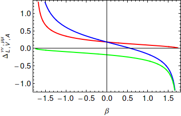
Figure 1: ΔLνν¯(Z)superscriptsubscriptΔ𝐿𝜈¯𝜈superscript𝑍\Delta_{L}^{\nu\bar{\nu}}(Z^{\prime}) (red), ΔVμμ¯(Z)superscriptsubscriptΔ𝑉𝜇¯𝜇superscript𝑍\Delta_{V}^{\mu\bar{\mu}}(Z^{\prime}) (blue) and ΔAμμ¯(Z)superscriptsubscriptΔ𝐴𝜇¯𝜇superscript𝑍\Delta_{A}^{\mu\bar{\mu}}(Z^{\prime}) (green) as functions of β𝛽\beta for sW2=0.249superscriptsubscript𝑠𝑊20.249s_{W}^{2}=0.249 and g=0.633𝑔0.633g=0.633. This plot applies to β3𝛽3\beta\not=\sqrt{3}.


In Fig. 1 we show ΔLνν¯(Z)superscriptsubscriptΔ𝐿𝜈¯𝜈superscript𝑍\Delta_{L}^{\nu\bar{\nu}}(Z^{\prime}), ΔVμμ¯(Z)superscriptsubscriptΔ𝑉𝜇¯𝜇superscript𝑍\Delta_{V}^{\mu\bar{\mu}}(Z^{\prime}) and ΔAμμ¯(Z)superscriptsubscriptΔ𝐴𝜇¯𝜇superscript𝑍\Delta_{A}^{\mu\bar{\mu}}(Z^{\prime}) as functions of β𝛽\beta for sW2=0.249superscriptsubscript𝑠𝑊20.249s_{W}^{2}=0.249 and g=0.633𝑔0.633g=0.633 corresponding to MZ=3TeVsubscript𝑀superscript𝑍3TeVM_{Z^{\prime}}=3\,{\rm TeV}. We observe the following features:

  • ΔLνν¯(Z)superscriptsubscriptΔ𝐿𝜈¯𝜈superscript𝑍\Delta_{L}^{\nu\bar{\nu}}(Z^{\prime}) and ΔAμμ¯(Z)superscriptsubscriptΔ𝐴𝜇¯𝜇superscript𝑍\Delta_{A}^{\mu\bar{\mu}}(Z^{\prime}) have definitive signs in the full range of β𝛽\beta: positive and negative, respectively.

  • ΔVμμ¯(Z)superscriptsubscriptΔ𝑉𝜇¯𝜇superscript𝑍\Delta_{V}^{\mu\bar{\mu}}(Z^{\prime}) can have both signs and for fixed |β|𝛽|\beta| its magnitude is larger for β<0𝛽0\beta<0. In fact the models with negative β𝛽\beta are then favoured by the BdKμ+μsubscript𝐵𝑑superscript𝐾superscript𝜇superscript𝜇B_{d}\to K^{*}\mu^{+}\mu^{-} anomalies. As noticed in [14] in this case in the limit of CMFV one automatically obtains C9NP<0subscriptsuperscript𝐶NP90C^{\rm NP}_{9}<0 as required by experiment. If there are new sources of flavour violation represented by the matrix VLsubscript𝑉𝐿V_{L} then the oasis in the space of new parameters has to be chosen for which in the case of negative β𝛽\beta one still has Re(C9NP)<0ResubscriptsuperscriptCNP90\rm{Re}(C^{\rm NP}_{9})<0. This will in turn have consequences for other processes as we will see below.

2.3 Various 331 models

It is instructive to list the values of the resulting couplings for the models with n=1,2,3𝑛123n=1,2,3 in (11). We do this for flavour diagonal couplings in Table 1 for sW2=0.249superscriptsubscript𝑠𝑊20.249s_{W}^{2}=0.249 and g=0.633𝑔0.633g=0.633 valid at MZ=3TeVsubscript𝑀superscript𝑍3TeVM_{Z^{\prime}}=3\,{\rm TeV} except for n=3𝑛3n=3, where we use MZ=2TeVsubscript𝑀superscript𝑍2TeVM_{Z^{\prime}}=2\,{\rm TeV} in order not to be too close to the Landau singularity. In Appendix A we give explicit formulae for these couplings in terms of sin2θWsuperscript2subscript𝜃𝑊\sin^{2}\theta_{W} as well as expressions for flavour violating couplings. Here and in Appendix A we give also Z𝑍Z-couplings.

β𝛽\beta in Zsuperscript𝑍Z^{\prime} couplings Z𝑍Z couplings
1/3131/\sqrt{3} 1/313-1/\sqrt{3} 2/3232/\sqrt{3} 2/323-2/\sqrt{3} 33\sqrt{3} 33-\sqrt{3}
ΔLuu¯superscriptsubscriptΔ𝐿𝑢¯𝑢\Delta_{L}^{u{\bar{u}}} -0.172 -0.215 -0.191 -0.299 -0.849 -1.672 0.257
ΔRuu¯superscriptsubscriptΔ𝑅𝑢¯𝑢\Delta_{R}^{u{\bar{u}}} 0.086 -0.086 0.216 -0.216 1.645 -1.645 -0.115
ΔVuu¯superscriptsubscriptΔ𝑉𝑢¯𝑢\Delta_{V}^{u{\bar{u}}} -0.087 -0.301 0.026 -0.515 0.796 -3.316 0.143
ΔAuu¯superscriptsubscriptΔ𝐴𝑢¯𝑢\Delta_{A}^{u{\bar{u}}} 0.258 0.130 0.407 0.082 2.494 0.027 -0.372
ΔLdd¯superscriptsubscriptΔ𝐿𝑑¯𝑑\Delta_{L}^{d{\bar{d}}} -0.172 -0.215 -0.191 -0.299 -0.849 -1.672 -0.315
ΔRdd¯superscriptsubscriptΔ𝑅𝑑¯𝑑\Delta_{R}^{d{\bar{d}}} -0.043 0.043 -0.108 0.108 -0.822 0.822 0.057
ΔVdd¯superscriptsubscriptΔ𝑉𝑑¯𝑑\Delta_{V}^{d{\bar{d}}} -0.215 -0.172 -0.299 -0.191 -1.672 -0.849 -0.257
ΔAdd¯superscriptsubscriptΔ𝐴𝑑¯𝑑\Delta_{A}^{d{\bar{d}}} 0.130 0.258 0.082 0.407 0.027 2.494 0.372
ΔLμμ¯superscriptsubscriptΔ𝐿𝜇¯𝜇\Delta_{L}^{\mu{\bar{\mu}}} 0.130 0.258 0.082 0.407 0.027 2.494 -0.199
ΔRμμ¯superscriptsubscriptΔ𝑅𝜇¯𝜇\Delta_{R}^{\mu{\bar{\mu}}} -0.128 0.128 -0.324 0.324 0.054 2.467 0.172
ΔVμμ¯superscriptsubscriptΔ𝑉𝜇¯𝜇\Delta_{V}^{\mu{\bar{\mu}}} 0.001 0.386 -0.242 0.731 0.080 4.961 -0.028
ΔAμμ¯superscriptsubscriptΔ𝐴𝜇¯𝜇\Delta_{A}^{\mu{\bar{\mu}}} -0.258 -0.130 -0.407 -0.082 0.027 -0.027 0.372
ΔLνν¯superscriptsubscriptΔ𝐿𝜈¯𝜈\Delta_{L}^{\nu{\bar{\nu}}} 0.130 0.258 0.082 0.407 0.027 2.494 0.372
Table 1: Diagonal Zsuperscript𝑍Z^{\prime} couplings to fermions for different β𝛽\beta and SM Z𝑍Z couplings to fermions (last column). We have used sin2θW=0.249superscript2subscript𝜃𝑊0.249\sin^{2}\theta_{W}=0.249 for β=±1/3𝛽plus-or-minus13\beta=\pm 1/\sqrt{3} and β=±2/3𝛽plus-or-minus23\beta=\pm 2/\sqrt{3}, sin2θW=0.246superscript2subscript𝜃𝑊0.246\sin^{2}\theta_{W}=0.246 for β=±3𝛽plus-or-minus3\beta=\pm\sqrt{3} and sin2θW=0.231superscript2subscript𝜃𝑊0.231\sin^{2}\theta_{W}=0.231 for Z𝑍Z-couplings.


3 Master formulae for one-loop functions and Wilson coefficients

3.1 New physics contributions

We collect here for completeness the corrections to SM one-loop functions and relevant Wilson coefficients as functions of the couplings listed in the previous section.

In the case of ΔF=2Δ𝐹2\Delta F=2 transitions governed by the function S𝑆S we have

ΔS(Bq)=[ΔLbq(Z)λt(q)]24r~MZ2gSM2,ΔS(K)=[ΔLsd(Z)λt(K)]24r~MZ2gSM2formulae-sequenceΔ𝑆subscript𝐵𝑞superscriptdelimited-[]superscriptsubscriptΔ𝐿𝑏𝑞superscript𝑍superscriptsubscript𝜆𝑡𝑞24~𝑟subscriptsuperscript𝑀2superscript𝑍superscriptsubscript𝑔SM2Δ𝑆𝐾superscriptdelimited-[]superscriptsubscriptΔ𝐿𝑠𝑑superscript𝑍superscriptsubscript𝜆𝑡𝐾24~𝑟subscriptsuperscript𝑀2superscript𝑍superscriptsubscript𝑔SM2\Delta S(B_{q})=\left[\frac{\Delta_{L}^{bq}(Z^{\prime})}{\lambda_{t}^{(q)}}\right]^{2}\frac{4\tilde{r}}{M^{2}_{Z^{\prime}}g_{\text{SM}}^{2}},\qquad\Delta S(K)=\left[\frac{\Delta_{L}^{sd}(Z^{\prime})}{\lambda_{t}^{(K)}}\right]^{2}\frac{4\tilde{r}}{M^{2}_{Z^{\prime}}g_{\text{SM}}^{2}} (20)

where

gSM2=4GF2α2πsin2θW,λi(K)=VisVid,λt(q)=VtbVtqformulae-sequencesuperscriptsubscript𝑔SM24subscript𝐺𝐹2𝛼2𝜋superscript2subscript𝜃𝑊formulae-sequencesubscriptsuperscript𝜆𝐾𝑖superscriptsubscript𝑉𝑖𝑠subscript𝑉𝑖𝑑superscriptsubscript𝜆𝑡𝑞superscriptsubscript𝑉𝑡𝑏subscript𝑉𝑡𝑞g_{\text{SM}}^{2}=4\frac{G_{F}}{\sqrt{2}}\frac{\alpha}{2\pi\sin^{2}\theta_{W}}\,,\qquad\lambda^{(K)}_{i}=V_{is}^{*}V_{id},\qquad\lambda_{t}^{(q)}=V_{tb}^{*}V_{tq} (21)

and r~~𝑟\tilde{r} is a QCD factor calculated in [2]. One finds r~=0.965~𝑟0.965\tilde{r}=0.965, r~=0.953~𝑟0.953\tilde{r}=0.953 and r~=0.925~𝑟0.925\tilde{r}=0.925 for MZ=2,3,10TeVsubscript𝑀superscript𝑍2310TeVM_{Z^{\prime}}=2,~{}3,~{}10\,{\rm TeV}, respectively. It should be remarked that gSM2superscriptsubscript𝑔SM2g_{\text{SM}}^{2} and sin2θWsuperscript2subscript𝜃𝑊\sin^{2}\theta_{W} appearing outside the Zsuperscript𝑍Z^{\prime} couplings, like in (26) and (27) below, should be evaluated at MZsubscript𝑀𝑍M_{Z} with input values given in Table 3 as they are just related to the overall normalization of Wilson coefficients and rescale relative to SM contributions.

For decays Bqμ+μsubscript𝐵𝑞superscript𝜇superscript𝜇B_{q}\to\mu^{+}\mu^{-} with q=d,s𝑞𝑑𝑠q=d,s governed by the function Y𝑌Y one has

ΔY(Bq)=[ΔAμμ¯(Z)MZ2gSM2]ΔLqb(Z)VtqVtbΔ𝑌subscript𝐵𝑞delimited-[]superscriptsubscriptΔ𝐴𝜇¯𝜇superscript𝑍superscriptsubscript𝑀superscript𝑍2subscriptsuperscript𝑔2SMsuperscriptsubscriptΔ𝐿𝑞𝑏superscript𝑍superscriptsubscript𝑉𝑡𝑞subscript𝑉𝑡𝑏\Delta Y(B_{q})=\left[\frac{\Delta_{A}^{\mu\bar{\mu}}(Z^{\prime})}{M_{Z^{\prime}}^{2}g^{2}_{\rm SM}}\right]\frac{\Delta_{L}^{qb}(Z^{\prime})}{V_{tq}^{\ast}V_{tb}} (22)

and for KLμ+μsubscript𝐾𝐿superscript𝜇superscript𝜇K_{L}\to\mu^{+}\mu^{-}

ΔY(K)=[ΔAμμ¯(Z)MZ2gSM2]ΔLsd(Z)VtsVtd.Δ𝑌𝐾delimited-[]superscriptsubscriptΔ𝐴𝜇¯𝜇superscript𝑍superscriptsubscript𝑀superscript𝑍2subscriptsuperscript𝑔2SMsuperscriptsubscriptΔ𝐿𝑠𝑑superscript𝑍superscriptsubscript𝑉𝑡𝑠subscript𝑉𝑡𝑑\Delta Y(K)=\left[\frac{\Delta_{A}^{\mu\bar{\mu}}(Z^{\prime})}{M_{Z^{\prime}}^{2}g^{2}_{\rm SM}}\right]\frac{\Delta_{L}^{sd}(Z^{\prime})}{V_{ts}^{\ast}V_{td}}. (23)

Similarly for bqνν¯𝑏𝑞𝜈¯𝜈b\to q\nu\bar{\nu} transitions governed by the function X𝑋X one finds

ΔX(Bq)=[ΔLνν(Z)gSM2MZ2]ΔLqb(Z)VtqVtbΔ𝑋subscript𝐵𝑞delimited-[]superscriptsubscriptΔ𝐿𝜈𝜈superscript𝑍subscriptsuperscript𝑔2SMsuperscriptsubscript𝑀superscript𝑍2superscriptsubscriptΔ𝐿𝑞𝑏superscript𝑍superscriptsubscript𝑉𝑡𝑞subscript𝑉𝑡𝑏\Delta X(B_{q})=\left[\frac{\Delta_{L}^{\nu\nu}(Z^{\prime})}{g^{2}_{\rm SM}M_{Z^{\prime}}^{2}}\right]\frac{\Delta_{L}^{qb}(Z^{\prime})}{V_{tq}^{\ast}V_{tb}} (24)

and for K+π+νν¯superscript𝐾superscript𝜋𝜈¯𝜈K^{+}\rightarrow\pi^{+}\nu\bar{\nu} and KLπ0νν¯subscript𝐾𝐿superscript𝜋0𝜈¯𝜈K_{L}\rightarrow\pi^{0}\nu\bar{\nu}

ΔX(K)=[ΔLνν¯(Z)gSM2MZ2]ΔLsd(Z)VtsVtd.Δ𝑋𝐾delimited-[]superscriptsubscriptΔ𝐿𝜈¯𝜈superscript𝑍subscriptsuperscript𝑔2SMsuperscriptsubscript𝑀superscript𝑍2superscriptsubscriptΔ𝐿𝑠𝑑superscript𝑍superscriptsubscript𝑉𝑡𝑠subscript𝑉𝑡𝑑\Delta X(K)=\left[\frac{\Delta_{L}^{\nu\bar{\nu}}(Z^{\prime})}{g^{2}_{\rm SM}M_{Z^{\prime}}^{2}}\right]\frac{\Delta_{L}^{sd}(Z^{\prime})}{V_{ts}^{*}V_{td}}. (25)

The corrections from NP to the Wilson coefficients C9subscript𝐶9C_{9} and C10subscript𝐶10C_{10} relevant for bsμ+μ𝑏𝑠superscript𝜇superscript𝜇b\to s\mu^{+}\mu^{-} transitions and used in the recent literature are given as follows333The coefficients CVsubscript𝐶𝑉C_{V} and CAsubscript𝐶𝐴C_{A} in [2] are obtained by multiplying C9subscript𝐶9C_{9} and C10subscript𝐶10C_{10} by sinθW2superscriptsubscript𝜃𝑊2\sin\theta_{W}^{2}, respectively.

sin2θWC9NPsuperscript2subscript𝜃𝑊subscriptsuperscript𝐶NP9\displaystyle\sin^{2}\theta_{W}C^{\rm NP}_{9} =1gSM2MZ2ΔLsb(Z)ΔVμμ¯(Z)VtsVtb,absent1superscriptsubscript𝑔SM2superscriptsubscript𝑀superscript𝑍2superscriptsubscriptΔ𝐿𝑠𝑏superscript𝑍superscriptsubscriptΔ𝑉𝜇¯𝜇superscript𝑍superscriptsubscript𝑉𝑡𝑠subscript𝑉𝑡𝑏\displaystyle=-\frac{1}{g_{\text{SM}}^{2}M_{Z^{\prime}}^{2}}\frac{\Delta_{L}^{sb}(Z^{\prime})\Delta_{V}^{\mu\bar{\mu}}(Z^{\prime})}{V_{ts}^{*}V_{tb}}, (26)
sin2θWC10NPsuperscript2subscript𝜃𝑊subscriptsuperscript𝐶NP10\displaystyle\sin^{2}\theta_{W}C^{\rm NP}_{10} =1gSM2MZ2ΔLsb(Z)ΔAμμ¯(Z)VtsVtb.absent1superscriptsubscript𝑔SM2superscriptsubscript𝑀superscript𝑍2superscriptsubscriptΔ𝐿𝑠𝑏superscript𝑍superscriptsubscriptΔ𝐴𝜇¯𝜇superscript𝑍superscriptsubscript𝑉𝑡𝑠subscript𝑉𝑡𝑏\displaystyle=-\frac{1}{g_{\text{SM}}^{2}M_{Z^{\prime}}^{2}}\frac{\Delta_{L}^{sb}(Z^{\prime})\Delta_{A}^{\mu\bar{\mu}}(Z^{\prime})}{V_{ts}^{*}V_{tb}}. (27)

3.2 Correlations

These formulae imply certain relations that are useful for the subsequent sections. First of all we have the ratio

R1=C9NPC10NP=Re(C9NP)Re(C10NP)=Im(C9NP)Im(C10NP)=ΔVμμ¯(Z)ΔAμμ¯(Z),subscript𝑅1subscriptsuperscript𝐶NP9subscriptsuperscript𝐶NP10ResubscriptsuperscriptCNP9ResubscriptsuperscriptCNP10ImsubscriptsuperscriptCNP9ImsubscriptsuperscriptCNP10superscriptsubscriptΔ𝑉𝜇¯𝜇superscript𝑍superscriptsubscriptΔ𝐴𝜇¯𝜇superscript𝑍R_{1}=\frac{C^{\rm NP}_{9}}{C^{\rm NP}_{10}}=\frac{\rm{Re}(C^{\rm NP}_{9})}{\rm{Re}(C^{\rm NP}_{10})}=\frac{\rm{Im}(C^{\rm NP}_{9})}{\rm{Im}(C^{\rm NP}_{10})}=\frac{\Delta_{V}^{\mu\bar{\mu}}(Z^{\prime})}{\Delta_{A}^{\mu\bar{\mu}}(Z^{\prime})}, (28)

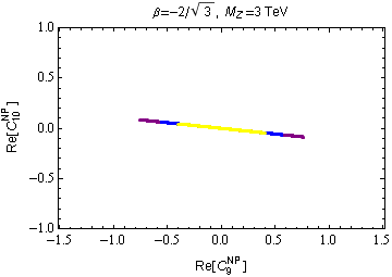
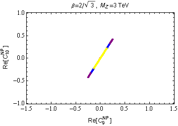
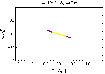
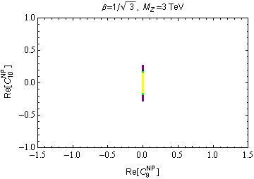
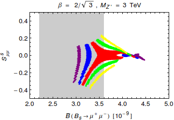
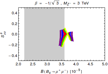
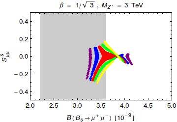
which involves only leptonic couplings and depends only on β𝛽\beta. This ratio is given in Table 2 for different values of β𝛽\beta and sW2=0.249superscriptsubscript𝑠𝑊20.249s_{W}^{2}=0.249 except for β=±3𝛽plus-or-minus3\beta=\pm\sqrt{3} where we use sW2=0.246superscriptsubscript𝑠𝑊20.246s_{W}^{2}=0.246. We observe that for β<0𝛽0\beta<0 these two coefficients are predicted to have opposite signs independently of the Zsuperscript𝑍Z^{\prime} couplings to quarks and as C10SMsubscriptsuperscript𝐶SM10C^{\rm SM}_{10} and C9SMsubscriptsuperscript𝐶SM9C^{\rm SM}_{9} have also opposite signs (see (53)). Re(C9NP)ResubscriptsuperscriptCNP9\rm{Re}(C^{\rm NP}_{9}) and NP contributions to ¯(Bsμ+μ)¯subscript𝐵𝑠superscript𝜇superscript𝜇\overline{\mathcal{B}}(B_{s}\to\mu^{+}\mu^{-}) are correlated with each other. This means that Re(C9NP)<0ResubscriptsuperscriptCNP90\rm{Re}(C^{\rm NP}_{9})<0 required by BdKμ+μsubscript𝐵𝑑superscript𝐾superscript𝜇superscript𝜇B_{d}\to K^{*}\mu^{+}\mu^{-} data implies for β<0𝛽0\beta<0 uniquely suppression of ¯(Bsμ+μ)¯subscript𝐵𝑠superscript𝜇superscript𝜇\overline{\mathcal{B}}(B_{s}\to\mu^{+}\mu^{-}) relative to its SM value which is favoured by the data. On the other hand for β=1/3𝛽13\beta=1/\sqrt{3} the ratio in (28) is tiny and for β>1/3𝛽13\beta>1/\sqrt{3} it is positive implying that NP contributions to ¯(Bsμ+μ)¯subscript𝐵𝑠superscript𝜇superscript𝜇\overline{\mathcal{B}}(B_{s}\to\mu^{+}\mu^{-}) and Re(C9NP)ResubscriptsuperscriptCNP9\rm{Re}(C^{\rm NP}_{9}) are anti-correlated with each other. Consequently in this case Re(C9NP)<0ResubscriptsuperscriptCNP90\rm{Re}(C^{\rm NP}_{9})<0 required by BdKμ+μsubscript𝐵𝑑superscript𝐾superscript𝜇superscript𝜇B_{d}\to K^{*}\mu^{+}\mu^{-} anomaly implies the enhancement of ¯(Bsμ+μ)¯subscript𝐵𝑠superscript𝜇superscript𝜇\overline{\mathcal{B}}(B_{s}\to\mu^{+}\mu^{-}) which is presently not supported by the data but this could change in the future. We will see all this explicitly in Section 6.

A complementary relation valid in any LHS model that this time does not depend on the lepton couplings is [13]

Im(C9NP)Re(C9NP)=Im(C10NP)Re(C10NP)=tan(δ2βs).ImsuperscriptsubscriptC9NPResuperscriptsubscriptC9NPImsuperscriptsubscriptC10NPResuperscriptsubscriptC10NPsubscript𝛿2subscript𝛽𝑠\frac{\rm{Im}(C_{9}^{\rm NP})}{\rm{Re}(C_{9}^{\rm NP})}=\frac{\rm{Im}(C_{10}^{\rm NP})}{\rm{Re}(C_{10}^{\rm NP})}=\tan(\delta_{2}-\beta_{s}). (29)

Two important points should be noticed here. These two ratios have to be equal to each other. Moreover they are the same in the two oases resulting from ΔF=2Δ𝐹2\Delta F=2 constraint.

Next the ratios

R2=ΔY(Bq)ΔX(Bq)=ΔY(K)ΔX(K)=ΔAμμ¯(Z)ΔLνν¯(Z)subscript𝑅2Δ𝑌subscript𝐵𝑞Δ𝑋subscript𝐵𝑞Δ𝑌𝐾Δ𝑋𝐾superscriptsubscriptΔ𝐴𝜇¯𝜇superscript𝑍superscriptsubscriptΔ𝐿𝜈¯𝜈superscript𝑍R_{2}=\frac{\Delta Y(B_{q})}{\Delta X(B_{q})}=\frac{\Delta Y(K)}{\Delta X(K)}=\frac{\Delta_{A}^{\mu\bar{\mu}}(Z^{\prime})}{\Delta_{L}^{\nu\bar{\nu}}(Z^{\prime})} (30)

express the relative importance of Zsuperscript𝑍Z^{\prime} contributions within a given meson system to decays with muons and neutrinos in the final state. While investigating the numbers for R2subscript𝑅2R_{2} in Table 2 we should recall that in the SM Y1.0𝑌1.0Y\approx 1.0 while X1.5𝑋1.5X\approx 1.5 which means that it is easier to make an impact on decays to muons. While from this ratio we cannot conclude whether a given branching ratio is enhanced or suppressed as the quark couplings cancel in this ratio, the message is clear:

  • For β>0𝛽0\beta>0 NP effects in decays to muons governed by axial-vector couplings are much larger than in decays to neutrinos, whereas the opposite is true for β<0𝛽0\beta<0. Therefore in the latter case which is chosen by the BdKμ+μsubscript𝐵𝑑superscript𝐾superscript𝜇superscript𝜇B_{d}\to K^{*}\mu^{+}\mu^{-} anomaly we can expect also measurable effects in decays to neutrinos.

  • Very importantly in all models, except β=3𝛽3\beta=\sqrt{3}, considered NP effects in Bsμ+μsubscript𝐵𝑠superscript𝜇superscript𝜇B_{s}\to\mu^{+}\mu^{-} are anti-correlated with the ones in bsνν¯𝑏𝑠𝜈¯𝜈b\to s\nu\bar{\nu} transitions.

β𝛽\beta 1/3131/\sqrt{3} 1/313-1/\sqrt{3} 2/3232/\sqrt{3} 2/323-2/\sqrt{3} 33\sqrt{3} 33-\sqrt{3}
R1subscript𝑅1R_{1} 0.0040.004-0.004 2.982.98-2.98 0.590.590.59 8.878.87-8.87 3.03.03.0 185.5185.5-185.5
R2subscript𝑅2R_{2} 1.991.99-1.99 0.500.50-0.50 4.944.94-4.94 0.200.20-0.20 1.01.01.0 0.010.01-0.01
R3subscript𝑅3R_{3} 0.610.610.61 1.221.221.22 0.390.390.39 1.931.931.93 0.130.130.13 11.811.811.8
R4subscript𝑅4R_{4} 0.670.670.67 0.670.670.67 0.420.420.42 0.420.420.42 0.0160.0160.016 0.0160.0160.016
R5subscript𝑅5R_{5} 0.500.500.50 1.001.001.00 0.250.250.25 1.251.251.25 0.0160.0160.016 1.491.491.49
R6subscript𝑅6R_{6} 1.001.00-1.00 0.500.50-0.50 1.251.25-1.25 0.250.25-0.25 0.0160.0160.016 0.0160.016-0.016
Table 2: Values of the ratios Risubscript𝑅𝑖R_{i} for different β𝛽\beta setting sin2θW=0.249superscript2subscript𝜃𝑊0.249\sin^{2}\theta_{W}=0.249 except for β=±3𝛽plus-or-minus3\beta=\pm\sqrt{3} where we use sW2=0.246superscriptsubscript𝑠𝑊20.246s_{W}^{2}=0.246.


Important are also the relations between the Zsuperscript𝑍Z^{\prime} contributions to ΔF=1Δ𝐹1\Delta F=1 (X𝑋X and Y𝑌Y functions) and ΔF=2Δ𝐹2\Delta F=2 (S𝑆S functions) observables. We have

ΔX(Bq)ΔS(Bq)=aqΔLνν¯(Z)2r~gSMMZ=aq0.085r~(3TeVMZ)R3Δ𝑋subscript𝐵𝑞Δ𝑆superscriptsubscript𝐵𝑞subscript𝑎𝑞superscriptsubscriptΔ𝐿𝜈¯𝜈superscript𝑍2~𝑟subscript𝑔SMsubscript𝑀superscript𝑍subscript𝑎𝑞0.085~𝑟3TeVsubscript𝑀superscript𝑍subscript𝑅3\frac{\Delta X(B_{q})}{\sqrt{\Delta S(B_{q})^{*}}}=a_{q}\frac{\Delta_{L}^{\nu\bar{\nu}}(Z^{\prime})}{2\sqrt{\tilde{r}}g_{\rm SM}M_{Z^{\prime}}}=-a_{q}\frac{0.085}{\sqrt{\tilde{r}}}\left(\frac{3\,{\rm TeV}}{M_{Z^{\prime}}}\right)R_{3} (31)

where

R3=[1(1+3β)sW2]1(1+β2)sW2,subscript𝑅3delimited-[]113𝛽superscriptsubscript𝑠𝑊211superscript𝛽2superscriptsubscript𝑠𝑊2R_{3}=\frac{\left[1-(1+\sqrt{3}\beta)s_{W}^{2}\right]}{\sqrt{1-(1+\beta^{2})s_{W}^{2}}}, (32)

ad=1subscript𝑎𝑑1a_{d}=1 and as=1subscript𝑎𝑠1a_{s}=-1.

We also have

ΔX(K)ΔS(K)=ΔX(Bs)ΔS(Bs).Δ𝑋𝐾Δ𝑆𝐾Δ𝑋subscript𝐵𝑠Δ𝑆superscriptsubscript𝐵𝑠\frac{\Delta X(K)}{\sqrt{\Delta S(K)}}=\frac{\Delta X(B_{s})}{\sqrt{\Delta S(B_{s})^{*}}}. (33)

As presently the constraints on 331 models are dominated by ΔF=2Δ𝐹2\Delta F=2 transitions we observe that for a given allowed size of ΔS(Bq)Δ𝑆subscript𝐵𝑞\Delta S(B_{q}), NP effects in the one-loop functions in question are proportional to 1/MZ1subscript𝑀superscript𝑍1/M_{Z^{\prime}} and this dependence is transfered to branching ratios in view of the fact that the dominant NP contributions are present there as interference between SM and NP contributions. That these effects are only suppressed like 1/MZ1subscript𝑀superscript𝑍1/M_{Z^{\prime}} and not like 1/MZ21subscriptsuperscript𝑀2superscript𝑍1/M^{2}_{Z^{\prime}} is the consequence of the increase with MZsubscript𝑀superscript𝑍M_{Z^{\prime}} of the allowed values of the couplings ΔLij(Z)superscriptsubscriptΔ𝐿𝑖𝑗superscript𝑍\Delta_{L}^{ij}(Z^{\prime}) extracted from ΔF=2Δ𝐹2\Delta F=2 observables, the point already stressed in [2]. In summary, denoting by Δ𝒪NP(MZ(i))Δsuperscript𝒪NPsuperscriptsubscript𝑀superscript𝑍𝑖\Delta\mathcal{O}^{\rm NP}(M_{Z^{\prime}}^{(i)}) NP contributions to a given ΔF=1Δ𝐹1\Delta F=1 observable in Bssubscript𝐵𝑠B_{s} and Bdsubscript𝐵𝑑B_{d} decays at two ((i=1,2)𝑖12(i=1,2) different values MZ(i)superscriptsubscript𝑀superscript𝑍𝑖M_{Z^{\prime}}^{(i)} we have a scaling law

Δ𝒪NP(MZ(1))=MZ(2)MZ(1)Δ𝒪NP(MZ(2)).Δsuperscript𝒪NPsuperscriptsubscript𝑀superscript𝑍1superscriptsubscript𝑀superscript𝑍2superscriptsubscript𝑀superscript𝑍1Δsuperscript𝒪NPsuperscriptsubscript𝑀superscript𝑍2\Delta\mathcal{O}^{\rm NP}(M_{Z^{\prime}}^{(1)})=\frac{M_{Z^{\prime}}^{(2)}}{M_{Z^{\prime}}^{(1)}}\Delta\mathcal{O}^{\rm NP}(M_{Z^{\prime}}^{(2)}). (34)

independently of β𝛽\beta and CBqsubscript𝐶subscript𝐵𝑞C_{B_{q}}. However the size of NP effect will depend on these two parameters as seen already in the case of β𝛽\beta in Table 2 and we will see this more explicitly in Section 6.

While this scaling law would apply in the case of the absence of correlations between Bqsubscript𝐵𝑞B_{q} and K𝐾K systems also to K𝐾K decays, in the 331 models the situation is different as we will now demonstrate. Indeed in these models there is a correlation between the Zsuperscript𝑍Z^{\prime} effects in ΔF=2Δ𝐹2\Delta F=2 master functions in different meson systems

ΔS(K)ΔS(Bd)ΔS(Bs)=MZ2gSM24r~[ΔLsd(Z)ΔLbd(Z)ΔLbs(Z)]2=3.68r~(MZ3TeV)2R4Δ𝑆𝐾Δ𝑆subscript𝐵𝑑Δ𝑆superscriptsubscript𝐵𝑠subscriptsuperscript𝑀2superscript𝑍subscriptsuperscript𝑔2SM4~𝑟superscriptdelimited-[]superscriptsubscriptΔ𝐿𝑠𝑑superscript𝑍superscriptsubscriptΔ𝐿𝑏𝑑superscript𝑍superscriptsubscriptΔ𝐿𝑏𝑠superscript𝑍23.68~𝑟superscriptsubscript𝑀superscript𝑍3TeV2subscript𝑅4\frac{\Delta S(K)}{\Delta S(B_{d})\Delta S(B_{s})^{*}}=\frac{M^{2}_{Z^{\prime}}g^{2}_{\rm SM}}{4\tilde{r}}\left[\frac{\Delta_{L}^{sd}(Z^{\prime})}{\Delta_{L}^{bd}(Z^{\prime})\Delta_{L}^{bs*}(Z^{\prime})}\right]^{2}=\frac{3.68}{\tilde{r}}\left(\frac{M_{Z^{\prime}}}{3\,{\rm TeV}}\right)^{2}R_{4} (35)

where

R4=1(1+β2)sW2.subscript𝑅411superscript𝛽2superscriptsubscript𝑠𝑊2R_{4}=1-(1+\beta^{2})s_{W}^{2}. (36)

Here and in following equations we set |Vtb|=1subscript𝑉𝑡𝑏1|V_{tb}|=1 and c~13=c~23=1subscript~𝑐13subscript~𝑐231\tilde{c}_{13}=\tilde{c}_{23}=1 if necessary. As the present data and lattice results imply |ΔS(Bq)|<0.25Δ𝑆subscript𝐵𝑞0.25|\Delta S(B_{q})|<0.25 and R4<0.7subscript𝑅40.7R_{4}<0.7 in all models, NP effects in εKsubscript𝜀𝐾\varepsilon_{K} are typically below 10%percent1010\%, which is welcome as with input parameters in Table 3 εKsubscript𝜀𝐾\varepsilon_{K} within the SM is in good agreement with the data.

Combining then relations (30), (31), (33) and (35) we find

ΔX(K)=0.16r~R5ΔS(Bd)ΔS(Bs),R5=R3R4formulae-sequenceΔ𝑋𝐾0.16~𝑟subscript𝑅5Δ𝑆subscript𝐵𝑑Δ𝑆superscriptsubscript𝐵𝑠subscript𝑅5subscript𝑅3subscript𝑅4\Delta X(K)=\frac{0.16}{\tilde{r}}R_{5}\sqrt{\Delta S(B_{d})\Delta S(B_{s})^{*}},\qquad R_{5}=R_{3}\sqrt{R_{4}} (37)
ΔY(K)=0.16r~R6ΔS(Bd)ΔS(Bs),R6=R2R3R4formulae-sequenceΔ𝑌𝐾0.16~𝑟subscript𝑅6Δ𝑆subscript𝐵𝑑Δ𝑆superscriptsubscript𝐵𝑠subscript𝑅6subscript𝑅2subscript𝑅3subscript𝑅4\Delta Y(K)=\frac{0.16}{\tilde{r}}R_{6}\sqrt{\Delta S(B_{d})\Delta S(B_{s})^{*}},\qquad R_{6}=R_{2}R_{3}\sqrt{R_{4}} (38)

with the values of R5subscript𝑅5R_{5} and R6subscript𝑅6R_{6} given in Table 2. We observe that ΔX(K)Δ𝑋𝐾\Delta X(K) and ΔY(K)Δ𝑌𝐾\Delta Y(K) do not depend on MZsubscript𝑀superscript𝑍M_{Z^{\prime}} when the parameters in VLsubscript𝑉𝐿V_{L} are constrained through Bs,d0B¯s,d0subscriptsuperscript𝐵0𝑠𝑑subscriptsuperscript¯𝐵0𝑠𝑑B^{0}_{s,d}-\bar{B}^{0}_{s,d} mixings. This fact has already been noticed in [2] but these explicit relations are new.

For the models considered in detail by us R5<1.3subscript𝑅51.3R_{5}<1.3 and as |ΔS(Bq)|<0.25Δ𝑆subscript𝐵𝑞0.25|\Delta S(B_{q})|<0.25 we find that |ΔX(K)|0.05Δ𝑋𝐾0.05|\Delta X(K)|\leq 0.05 which implies a correction to K+π+νν¯superscript𝐾superscript𝜋𝜈¯𝜈K^{+}\rightarrow\pi^{+}\nu\bar{\nu} and KLπ0νν¯subscript𝐾𝐿superscript𝜋0𝜈¯𝜈K_{L}\rightarrow\pi^{0}\nu\bar{\nu} of at most 10%percent1010\% at the level of the branching ratios.

As far as the Wilson coefficients C9NPsuperscriptsubscript𝐶9NPC_{9}^{\rm NP} and C10NPsuperscriptsubscript𝐶10NPC_{10}^{\rm NP} are concerned we have two important relations

(ΔS(Bq))=4r~gSM2MZ2sin4θW[C9NPΔVμμ¯(Z)]2=0.327[C9NPΔVμμ¯(Z)]2[MZ3TeV]2,superscriptΔ𝑆subscript𝐵𝑞4~𝑟subscriptsuperscript𝑔2SMsuperscriptsubscript𝑀superscript𝑍2superscript4subscript𝜃𝑊superscriptdelimited-[]superscriptsubscript𝐶9NPsuperscriptsubscriptΔ𝑉𝜇¯𝜇superscript𝑍20.327superscriptdelimited-[]superscriptsubscript𝐶9NPsuperscriptsubscriptΔ𝑉𝜇¯𝜇superscript𝑍2superscriptdelimited-[]subscript𝑀superscript𝑍3TeV2(\Delta S(B_{q}))^{*}=4\tilde{r}g^{2}_{\rm SM}M_{Z^{\prime}}^{2}\sin^{4}\theta_{W}\left[\frac{C_{9}^{\rm NP}}{\Delta_{V}^{\mu\bar{\mu}}(Z^{\prime})}\right]^{2}=0.327\left[\frac{C_{9}^{\rm NP}}{\Delta_{V}^{\mu\bar{\mu}}(Z^{\prime})}\right]^{2}\left[\frac{M_{Z^{\prime}}}{3\,{\rm TeV}}\right]^{2}, (39)
(ΔS(Bq))=4r~gSM2MZ2sin4θW[C10NPΔAμμ¯(Z)]2=0.327[C10NPΔAμμ¯(Z)]2[MZ3TeV]2,superscriptΔ𝑆subscript𝐵𝑞4~𝑟subscriptsuperscript𝑔2SMsuperscriptsubscript𝑀superscript𝑍2superscript4subscript𝜃𝑊superscriptdelimited-[]superscriptsubscript𝐶10NPsuperscriptsubscriptΔ𝐴𝜇¯𝜇superscript𝑍20.327superscriptdelimited-[]superscriptsubscript𝐶10NPsuperscriptsubscriptΔ𝐴𝜇¯𝜇superscript𝑍2superscriptdelimited-[]subscript𝑀superscript𝑍3TeV2(\Delta S(B_{q}))^{*}=4\tilde{r}g^{2}_{\rm SM}M_{Z^{\prime}}^{2}\sin^{4}\theta_{W}\left[\frac{C_{10}^{\rm NP}}{\Delta_{A}^{\mu\bar{\mu}}(Z^{\prime})}\right]^{2}=0.327\left[\frac{C_{10}^{\rm NP}}{\Delta_{A}^{\mu\bar{\mu}}(Z^{\prime})}\right]^{2}\left[\frac{M_{Z^{\prime}}}{3\,{\rm TeV}}\right]^{2}, (40)

which we have written in a form suitable for the analysis in Section 6. We recall that SSM=S0(xt)=2.31subscript𝑆SMsubscript𝑆0subscript𝑥𝑡2.31S_{\rm SM}=S_{0}(x_{t})=2.31. Both relations are valid for Bssubscript𝐵𝑠B_{s} and Bdsubscript𝐵𝑑B_{d} systems as indicated on the l.h.s of these equations and the Wilson coefficients on the r.h.s should be appropriately adjusted to the case considered.

The virtue of these relation is their independence of the new parameters in (15) so that for a given β𝛽\beta the size of C9NPsuperscriptsubscript𝐶9NPC_{9}^{\rm NP} and C10NPsuperscriptsubscript𝐶10NPC_{10}^{\rm NP} allowed by the ΔF=2Δ𝐹2\Delta F=2 constraints can be found. In particular in the case of a real C9NPsuperscriptsubscript𝐶9NPC_{9}^{\rm NP} and C10NPsuperscriptsubscript𝐶10NPC_{10}^{\rm NP}, corresponding to VL=VCKMsubscript𝑉𝐿subscript𝑉CKMV_{L}=V_{\rm CKM}, ΔS(Bq)Δ𝑆subscript𝐵𝑞\Delta S(B_{q}) and ΔMqΔsubscript𝑀𝑞\Delta M_{q} will be enhanced which is only allowed if the SM values of ΔMqΔsubscript𝑀𝑞\Delta M_{q} will turn out to be below the data. If this will not be the case the only solution is to misalign VLsubscript𝑉𝐿V_{L} and VCKMsubscript𝑉CKMV_{\rm CKM} which results in complex C9NPsuperscriptsubscript𝐶9NPC_{9}^{\rm NP} and C10NPsuperscriptsubscript𝐶10NPC_{10}^{\rm NP} and consequently novel CP-violating effects.

4 Crucial observables

4.1 𝚫𝑭=𝟐𝚫𝑭2\Delta F=2 observables

The 𝑩𝒔𝟎𝑩¯𝒔𝟎superscriptsubscript𝑩𝒔0superscriptsubscriptbold-¯𝑩𝒔0B_{s}^{0}-\bar{B}_{s}^{0} observables are fully described in 331 models by the function

𝑺(𝑩𝒔)=𝑺𝟎(𝒙𝒕)+𝚫𝑺(𝑩𝒔)|𝑺(𝑩𝒔)|𝒆𝒊𝟐𝝋𝑩𝒔,𝑺subscript𝑩𝒔subscript𝑺0subscript𝒙𝒕𝚫𝑺subscript𝑩𝒔𝑺subscript𝑩𝒔superscript𝒆𝒊2subscript𝝋subscript𝑩𝒔S(B_{s})=S_{0}(x_{t})+\Delta S(B_{s})\equiv|S(B_{s})|e^{-i2\varphi_{B_{s}}}, (41)

where 𝑺𝟎(𝒙𝒕)subscript𝑺0subscript𝒙𝒕S_{0}(x_{t}) is the real one-loop SM box function and the additional generally complex term has been given in (20).

The two observables of interest, 𝚫𝑴𝒔𝚫subscript𝑴𝒔\Delta M_{s} and 𝑺𝝍ϕsubscript𝑺𝝍bold-italic-ϕS_{\psi\phi} are then given by

𝚫𝑴𝒔=𝑮𝑭𝟐𝟔𝝅𝟐𝑴𝑾𝟐𝒎𝑩𝒔|𝑽𝒕𝒃𝑽𝒕𝒔|𝟐𝑭𝑩𝒔𝟐𝑩^𝑩𝒔𝜼𝑩|𝑺(𝑩𝒔)|𝚫subscript𝑴𝒔superscriptsubscript𝑮𝑭26superscript𝝅2superscriptsubscript𝑴𝑾2subscript𝒎subscript𝑩𝒔superscriptsubscriptsuperscript𝑽𝒕𝒃subscript𝑽𝒕𝒔2superscriptsubscript𝑭subscript𝑩𝒔2subscriptbold-^𝑩subscript𝑩𝒔subscript𝜼𝑩𝑺subscript𝑩𝒔\Delta M_{s}=\frac{G_{F}^{2}}{6\pi^{2}}M_{W}^{2}m_{B_{s}}|V^{*}_{tb}V_{ts}|^{2}F_{B_{s}}^{2}\hat{B}_{B_{s}}\eta_{B}|S(B_{s})|\, (42)

and

𝑺𝝍ϕ=𝐬𝐢𝐧(𝟐|𝜷𝒔|𝟐𝝋𝑩𝒔),𝑽𝒕𝒔=|𝑽𝒕𝒔|𝒆𝒊𝜷𝒔.formulae-sequencesubscript𝑺𝝍bold-italic-ϕ2subscript𝜷𝒔2subscript𝝋subscript𝑩𝒔subscript𝑽𝒕𝒔subscript𝑽𝒕𝒔superscript𝒆𝒊subscript𝜷𝒔S_{\psi\phi}=\sin(2|\beta_{s}|-2\varphi_{B_{s}})\,,\qquad V_{ts}=-|V_{ts}|e^{-i\beta_{s}}. (43)

with 𝜷𝒔𝟏similar-to-or-equalssubscript𝜷𝒔superscript1\beta_{s}\simeq-1^{\circ}\,.

In the case of 𝑩𝒅𝟎superscriptsubscript𝑩𝒅0B_{d}^{0} system the corresponding formulae are obtained from (41) and (42) by replacing 𝒔𝒔s by 𝒅𝒅d. Moreover (43) is replaced by

𝑺𝝍𝑲𝑺=𝐬𝐢𝐧(𝟐𝜷𝟐𝝋𝑩𝒅),𝑽𝒕𝒅=|𝑽𝒕𝒅|𝒆𝒊𝜷.formulae-sequencesubscript𝑺𝝍subscript𝑲𝑺2𝜷2subscript𝝋subscript𝑩𝒅subscript𝑽𝒕𝒅subscript𝑽𝒕𝒅superscript𝒆𝒊𝜷S_{\psi K_{S}}=\sin(2\beta-2\varphi_{B_{d}})\,,\qquad V_{td}=|V_{td}|e^{-i\beta}. (44)

With the input for |𝑽𝒖𝒃|subscript𝑽𝒖𝒃|V_{ub}| and |𝑽𝒄𝒃|subscript𝑽𝒄𝒃|V_{cb}| in Table 3 and 𝜸=𝟔𝟖𝜸superscript68\gamma=68^{\circ} there is a good agreement of the SM with data on 𝑺𝝍𝑲𝑺subscript𝑺𝝍subscript𝑲𝑺S_{\psi K_{S}} and 𝜺𝑲subscript𝜺𝑲\varepsilon_{K}.

In the SM one has444The central value of |Vts|subscript𝑉𝑡𝑠|V_{ts}| corresponds roughly to the central |Vcb|=0.0424subscript𝑉𝑐𝑏0.0424|V_{cb}|=0.0424 obtained from tree-level inclusive decays [38].

(𝚫𝑴𝒔)𝐒𝐌=18.8/𝐩𝐬[𝑩^𝑩𝒔𝑭𝑩𝒔𝟐𝟔𝟔𝐌𝐞𝐕]𝟐[𝑺𝟎(𝒙𝒕)2.31][|𝑽𝒕𝒔|0.0416]𝟐[𝜼𝑩0.55],subscript𝚫subscript𝑴𝒔𝐒𝐌bold-⋅18.8𝐩𝐬superscriptdelimited-[]subscriptbold-^𝑩subscript𝑩𝒔subscript𝑭subscript𝑩𝒔266𝐌𝐞𝐕2delimited-[]subscript𝑺0subscript𝒙𝒕2.31superscriptdelimited-[]subscript𝑽𝒕𝒔0.04162delimited-[]subscript𝜼𝑩0.55(\Delta M_{s})_{\rm SM}=18.8/{\rm ps}\cdot\left[\frac{\sqrt{\hat{B}_{B_{s}}}F_{B_{s}}}{266\,{\rm MeV}}\right]^{2}\left[\frac{S_{0}(x_{t})}{2.31}\right]\left[\frac{|V_{ts}|}{0.0416}\right]^{2}\left[\frac{\eta_{B}}{0.55}\right]\,, (45)
(𝚫𝑴𝒅)𝐒𝐌=0.54/𝐩𝐬[𝑩^𝑩𝒅𝑭𝑩𝒅𝟐𝟏𝟖𝐌𝐞𝐕]𝟐[𝑺𝟎(𝒙𝒕)2.31][|𝑽𝒕𝒅|8.8𝟏𝟎𝟑]𝟐[𝜼𝑩0.55].subscript𝚫subscript𝑴𝒅𝐒𝐌bold-⋅0.54𝐩𝐬superscriptdelimited-[]subscriptbold-^𝑩subscript𝑩𝒅subscript𝑭subscript𝑩𝒅218𝐌𝐞𝐕2delimited-[]subscript𝑺0subscript𝒙𝒕2.31superscriptdelimited-[]subscript𝑽𝒕𝒅bold-⋅8.8superscript1032delimited-[]subscript𝜼𝑩0.55(\Delta M_{d})_{\rm SM}=0.54/{\rm ps}\cdot\left[\frac{\sqrt{\hat{B}_{B_{d}}}F_{B_{d}}}{218\,{\rm MeV}}\right]^{2}\left[\frac{S_{0}(x_{t})}{2.31}\right]\left[\frac{|V_{td}|}{8.8\cdot 10^{-3}}\right]^{2}\left[\frac{\eta_{B}}{0.55}\right]\,. (46)

For the central values of the parameters in Table 3 there is a good agreement with the very accurate data [39]:

𝚫𝑴𝒔=17.69(𝟖)ps𝟏,𝚫𝑴𝒅=0.510(𝟒)ps𝟏,formulae-sequence𝚫subscript𝑴𝒔17.698superscriptps1𝚫subscript𝑴𝒅0.5104superscriptps1\Delta M_{s}=17.69(8)\,\text{ps}^{-1},\qquad\Delta M_{d}=0.510(4)\,\text{ps}^{-1}~{}, (47)

even if both central values are by 𝟓𝟔%5percent65-6\% above the data. With the most recent values from the Twisted Mass Collaboration [40]

𝑩^𝑩𝒔𝑭𝑩𝒔=𝟐𝟔𝟐(𝟏𝟎)𝐌𝐞𝐕,𝑩^𝑩𝒅𝑭𝑩𝒅=𝟐𝟏𝟔(𝟏𝟎)𝐌𝐞𝐕,formulae-sequencesubscriptbold-^𝑩subscript𝑩𝒔subscript𝑭subscript𝑩𝒔26210𝐌𝐞𝐕subscriptbold-^𝑩subscript𝑩𝒅subscript𝑭subscript𝑩𝒅21610𝐌𝐞𝐕\sqrt{\hat{B}_{B_{s}}}F_{B_{s}}=262(10)\,{\rm MeV},\qquad\sqrt{\hat{B}_{B_{d}}}F_{B_{d}}=216(10)\,{\rm MeV}, (48)

that are not yet included in the FLAG average, the central value of 𝚫𝑴𝒔𝚫subscript𝑴𝒔\Delta M_{s} would go down to 18.2/𝐩𝐬18.2𝐩𝐬18.2/{\rm ps}.

Concerning 𝑺𝝍ϕsubscript𝑺𝝍bold-italic-ϕS_{\psi\phi} and 𝑺𝝍𝑲𝑺subscript𝑺𝝍subscript𝑲𝑺S_{\psi K_{S}} we have

𝑺𝝍ϕ=(0.040.13+0.10),𝑺𝝍𝑲𝑺=0.679(𝟐𝟎)formulae-sequencesubscript𝑺𝝍bold-italic-ϕsubscriptsuperscript0.040.100.13subscript𝑺𝝍subscript𝑲𝑺0.67920S_{\psi\phi}=-\left(0.04^{+0.10}_{-0.13}\right),\qquad S_{\psi K_{S}}=0.679(20) (49)

with the second value known already for some time [39] and the first one being the most recent average from HFAG [39] close to the earlier result from the LHCb [41]. The first value is consistent with the SM expectation of 0.040.040.04. This is also the case of 𝑺𝝍𝑲𝑺subscript𝑺𝝍subscript𝑲𝑺S_{\psi K_{S}} for the values of |𝑽𝒖𝒃|subscript𝑽𝒖𝒃|V_{ub}| and |𝑽𝒄𝒃|subscript𝑽𝒄𝒃|V_{cb}| used by us.

4.2 𝒃𝒔𝝁+𝝁bold-→𝒃𝒔superscript𝝁superscript𝝁b\to s\mu^{+}\mu^{-} observables

The two Wilson coefficients that receive NP contributions in 331 models are 𝑪𝟗subscript𝑪9C_{9} and 𝑪𝟏𝟎subscript𝑪10C_{10}. We decompose them into the SM and NP contributions555These coefficients are defined as in [19] and the same definitions are used in [10, 11].:

𝑪𝟗=𝑪𝟗𝐒𝐌+𝑪𝟗𝐍𝐏,𝑪𝟏𝟎=𝑪𝟏𝟎𝐒𝐌+𝑪𝟏𝟎𝐍𝐏,formulae-sequencesubscript𝑪9superscriptsubscript𝑪9𝐒𝐌superscriptsubscript𝑪9𝐍𝐏subscript𝑪10superscriptsubscript𝑪10𝐒𝐌superscriptsubscript𝑪10𝐍𝐏C_{9}=C_{9}^{\rm SM}+C_{9}^{\rm NP},\qquad C_{10}=C_{10}^{\rm SM}+C_{10}^{\rm NP}, (50)

where NP contributions have been given in (26) and (27) and the SM contributions are given as follows

𝐬𝐢𝐧𝟐𝜽𝑾𝑪𝟗𝐒𝐌superscript2subscript𝜽𝑾subscriptsuperscript𝑪𝐒𝐌9\displaystyle\sin^{2}\theta_{W}C^{\rm SM}_{9} =𝐬𝐢𝐧𝟐𝜽𝑾𝑷𝟎𝐍𝐃𝐑+[𝜼𝐞𝐟𝐟𝒀𝟎(𝒙𝒕)𝟒𝐬𝐢𝐧𝟐𝜽𝑾𝒁𝟎(𝒙𝒕)],absentsuperscript2subscript𝜽𝑾superscriptsubscript𝑷0𝐍𝐃𝐑delimited-[]subscript𝜼𝐞𝐟𝐟subscript𝒀0subscript𝒙𝒕4superscript2subscript𝜽𝑾subscript𝒁0subscript𝒙𝒕\displaystyle=\sin^{2}\theta_{W}P_{0}^{\rm NDR}+[\eta_{\rm eff}Y_{0}(x_{t})-4\sin^{2}\theta_{W}Z_{0}(x_{t})], (51)
𝐬𝐢𝐧𝟐𝜽𝑾𝑪𝟏𝟎𝐒𝐌superscript2subscript𝜽𝑾subscriptsuperscript𝑪𝐒𝐌10\displaystyle\sin^{2}\theta_{W}C^{\rm SM}_{10} =𝜼𝐞𝐟𝐟𝒀𝟎(𝒙𝒕)absentsubscript𝜼𝐞𝐟𝐟subscript𝒀0subscript𝒙𝒕\displaystyle=-\eta_{\rm eff}Y_{0}(x_{t}) (52)

with all the entries given in [19, 13] except for 𝜼𝐞𝐟𝐟subscript𝜼𝐞𝐟𝐟\eta_{\rm eff} which is new and given below. We have then

𝑪𝟗𝐒𝐌4.1,𝑪𝟏𝟎𝐒𝐌4.1.formulae-sequencesubscriptsuperscript𝑪𝐒𝐌94.1subscriptsuperscript𝑪𝐒𝐌104.1C^{\rm SM}_{9}\approx 4.1,\qquad C^{\rm SM}_{10}\approx-4.1~{}. (53)

In the case of 𝑩𝒔𝝁+𝝁bold-→subscript𝑩𝒔superscript𝝁superscript𝝁B_{s}\to\mu^{+}\mu^{-} decay one has [42, 43, 44]

𝓑¯(𝑩𝒔𝝁+𝝁)𝓑¯(𝑩𝒔𝝁+𝝁)𝐒𝐌=[𝟏+𝓐𝚫𝚪𝝁𝝁𝒚𝒔𝟏+𝒚𝒔]|𝑷|𝟐,𝑷=𝑪𝟏𝟎𝑪𝟏𝟎𝐒𝐌|𝑷|𝒆𝒊𝝋𝑷,formulae-sequencebold-¯𝓑bold-→subscript𝑩𝒔superscript𝝁superscript𝝁bold-¯𝓑subscriptbold-→subscript𝑩𝒔superscript𝝁superscript𝝁𝐒𝐌delimited-[]1subscriptsuperscript𝓐𝝁𝝁𝚫𝚪subscript𝒚𝒔1subscript𝒚𝒔superscript𝑷2𝑷subscript𝑪10superscriptsubscript𝑪10𝐒𝐌𝑷superscript𝒆𝒊subscript𝝋𝑷\frac{\overline{\mathcal{B}}(B_{s}\to\mu^{+}\mu^{-})}{\overline{\mathcal{B}}(B_{s}\to\mu^{+}\mu^{-})_{\rm SM}}=\left[\frac{1+{\cal A}^{\mu\mu}_{\Delta\Gamma}\,y_{s}}{1+y_{s}}\right]|P|^{2},\qquad P=\frac{C_{10}}{C_{10}^{\rm SM}}\equiv|P|e^{i\varphi_{P}}, (54)

where

𝓑¯(𝑩𝒔𝝁+𝝁)SM=𝟏𝟏𝒚𝒔𝓑(𝑩𝒔𝝁+𝝁)SM,bold-¯𝓑subscriptbold-→subscript𝑩𝒔superscript𝝁superscript𝝁SM11subscript𝒚𝒔𝓑subscriptbold-→subscript𝑩𝒔superscript𝝁superscript𝝁SM\displaystyle\overline{\mathcal{B}}(B_{s}\to\mu^{+}\mu^{-})_{\text{SM}}=\frac{1}{1-y_{s}}\mathcal{B}(B_{s}\to\mu^{+}\mu^{-})_{\text{SM}}\,, (55)
𝓑(𝑩𝒔𝝁+𝝁)SM=𝝉𝑩𝒔𝑮𝑭𝟐𝝅(𝜶𝟒𝝅𝐬𝐢𝐧𝟐𝜽𝑾)𝟐𝑭𝑩𝒔𝟐𝒎𝝁𝟐𝒎𝑩𝒔𝟏𝟒𝒎𝝁𝟐𝒎𝑩𝒔𝟐|𝑽𝒕𝒃𝑽𝒕𝒔|𝟐𝜼eff𝟐𝒀𝟎(𝒙𝒕)𝟐,𝓑subscriptbold-→subscript𝑩𝒔superscript𝝁superscript𝝁SMsubscript𝝉subscript𝑩𝒔superscriptsubscript𝑮𝑭2𝝅superscript𝜶4𝝅superscript2subscript𝜽𝑾2superscriptsubscript𝑭subscript𝑩𝒔2superscriptsubscript𝒎𝝁2subscript𝒎subscript𝑩𝒔14superscriptsubscript𝒎𝝁2superscriptsubscript𝒎subscript𝑩𝒔2superscriptsuperscriptsubscript𝑽𝒕𝒃subscript𝑽𝒕𝒔2superscriptsubscript𝜼eff2subscript𝒀0superscriptsubscript𝒙𝒕2\displaystyle\mathcal{B}(B_{s}\to\mu^{+}\mu^{-})_{\text{SM}}=\tau_{B_{s}}\frac{G_{F}^{2}}{\pi}\left(\frac{\alpha}{4\pi\sin^{2}\theta_{W}}\right)^{2}F_{B_{s}}^{2}m_{\mu}^{2}m_{B_{s}}\sqrt{1-\frac{4m_{\mu}^{2}}{m_{B_{s}}^{2}}}\left|V_{tb}^{*}V_{ts}\right|^{2}\eta_{\text{eff}}^{2}Y_{0}(x_{t})^{2}\,, (56)
𝓐𝚫𝚪𝝁𝝁=𝐜𝐨𝐬(𝟐𝝋𝑷𝟐𝝋𝑩𝒔),𝒚𝒔𝝉𝑩𝒔𝚫𝚪𝒔𝟐=0.062±0.009formulae-sequencesubscriptsuperscript𝓐𝝁𝝁𝚫𝚪2subscript𝝋𝑷2subscript𝝋subscript𝑩𝒔subscript𝒚𝒔subscript𝝉subscript𝑩𝒔𝚫subscript𝚪𝒔2plus-or-minus0.0620.009\displaystyle{\cal A}^{\mu\mu}_{\Delta\Gamma}=\cos(2\varphi_{P}-2\varphi_{B_{s}}),\qquad y_{s}\equiv\tau_{B_{s}}\frac{\Delta\Gamma_{s}}{2}=0.062\pm 0.009 (57)

with the later value being the latest world average [39]. The bar indicates that 𝚫𝚪𝒔𝚫subscript𝚪𝒔\Delta\Gamma_{s} effects have been taken into account. In the SM and CMFV 𝓐𝚫𝚪𝝁𝝁=𝟏subscriptsuperscript𝓐𝝁𝝁𝚫𝚪1{\cal A}^{\mu\mu}_{\Delta\Gamma}=1 but in the 331 models it is slightly smaller and we take this effect into account. Generally as shown in [44] 𝓐𝚫𝚪𝝁𝝁subscriptsuperscript𝓐𝝁𝝁𝚫𝚪{\cal A}^{\mu\mu}_{\Delta\Gamma} can serve to test NP models as it can be determined in time-dependent measurements [42, 43]. Of interest is also the CP asymmetry

𝑺𝝁𝝁𝒔=𝐬𝐢𝐧(𝟐𝝋𝑷𝟐𝝋𝑩𝒔),subscriptsuperscript𝑺𝒔𝝁𝝁2subscript𝝋𝑷2subscript𝝋subscript𝑩𝒔S^{s}_{\mu\mu}=\sin(2\varphi_{P}-2\varphi_{B_{s}}), (58)

which has been studied in detail in [19, 44] in the context of 𝒁superscript𝒁bold-′Z^{\prime} models. In the case of 𝑩𝒅𝝁+𝝁bold-→subscript𝑩𝒅superscript𝝁superscript𝝁B_{d}\to\mu^{+}\mu^{-} decay the formulae given above apply with 𝒔𝒔s replaced by 𝒅𝒅d and 𝒚𝒅𝟎subscript𝒚𝒅0y_{d}\approx 0. Explicit formulae for 𝑩𝒅𝝁+𝝁bold-→subscript𝑩𝒅superscript𝝁superscript𝝁B_{d}\to\mu^{+}\mu^{-} can be found in [19].

Concerning the the status of the branching ratios for 𝑩𝒔,𝒅𝝁+𝝁bold-→subscript𝑩𝒔𝒅superscript𝝁superscript𝝁B_{s,d}\to\mu^{+}\mu^{-} decays we have

𝓑¯(𝑩𝒔𝝁+𝝁)𝐒𝐌=(3.65±0.23)𝟏𝟎𝟗,𝓑¯(𝑩𝒔𝝁+𝝁)=(2.9±0.7)×𝟏𝟎𝟗,formulae-sequencebold-¯𝓑subscriptbold-→subscript𝑩𝒔superscript𝝁superscript𝝁𝐒𝐌bold-⋅plus-or-minus3.650.23superscript109bold-¯𝓑bold-→subscript𝑩𝒔superscript𝝁superscript𝝁plus-or-minus2.90.7superscript109\overline{\mathcal{B}}(B_{s}\to\mu^{+}\mu^{-})_{\rm SM}=(3.65\pm 0.23)\cdot 10^{-9},\quad\overline{\mathcal{B}}(B_{s}\to\mu^{+}\mu^{-})=(2.9\pm 0.7)\times 10^{-9}, (59)
𝓑(𝑩𝒅𝝁+𝝁)𝐒𝐌=(1.06±0.09)×𝟏𝟎𝟏𝟎,𝓑(𝑩𝒅𝝁+𝝁)=(3.61.4+1.6)×𝟏𝟎𝟏𝟎.formulae-sequence𝓑subscriptbold-→subscript𝑩𝒅superscript𝝁superscript𝝁𝐒𝐌plus-or-minus1.060.09superscript1010𝓑bold-→subscript𝑩𝒅superscript𝝁superscript𝝁subscriptsuperscript3.61.61.4superscript1010\mathcal{B}(B_{d}\to\mu^{+}\mu^{-})_{\rm SM}=(1.06\pm 0.09)\times 10^{-10},\quad\mathcal{B}(B_{d}\to\mu^{+}\mu^{-})=\left(3.6^{+1.6}_{-1.4}\right)\times 10^{-10}. (60)

The SM values are based on [45] in which NLO corrections of electroweak origin [46] and QCD corrections up to NNLO [47] have been taken into account. These values are rather close to the ones presented previously by us [48, 44] but the inclusion of these new higher order corrections that were missing until now reduced significantly various scale uncertainties so that non-parametric uncertainties in both branching ratios are below 𝟐%percent22\%. The experimental data are the most recent averages of the results from LHCb and CMS [4, 5, 6].

The calculations performed in [46, 47] are very involved and in analogy to the QCD factors, like 𝜼𝑩subscript𝜼𝑩\eta_{B} and 𝜼𝟏𝟑subscript𝜼13\eta_{1-3} in 𝚫𝑭=𝟐𝚫𝑭2\Delta F=2 processes, we find it useful to include all QCD and electroweak corrections into 𝜼𝐞𝐟𝐟subscript𝜼𝐞𝐟𝐟\eta_{\rm eff} introduced in (52) that without these corrections would be equal to unity. Inspecting the analytic formulae in [45] one finds then

𝜼𝐞𝐟𝐟=0.9882±0.0024.subscript𝜼𝐞𝐟𝐟plus-or-minus0.98820.0024\eta_{\rm eff}=0.9882\pm 0.0024~{}. (61)

The small departure of 𝜼𝐞𝐟𝐟subscript𝜼𝐞𝐟𝐟\eta_{\rm eff} from unity was already anticipated in [49, 48] but only the calculations in [45, 46, 47] could put these expectations and conjectures on firm footing. Indeed, in order to end up with such a simple result it was crucial to perform such involved calculations as these small corrections are only valid for particular definitions of the top-quark mass and of other electroweak parameters involved. In particular one has to use in 𝒀𝟎(𝒙𝒕)subscript𝒀0subscript𝒙𝒕Y_{0}(x_{t}) the 𝐌𝐒¯bold-¯𝐌𝐒\overline{\rm MS}-renormalized top-quark mass 𝒎𝒕(𝒎𝒕)subscript𝒎𝒕subscript𝒎𝒕m_{t}(m_{t}) with respect to QCD but on-shell with respect to electroweak interactions. This means 𝒎𝒕(𝒎𝒕)=163.5𝐆𝐞𝐕subscript𝒎𝒕subscript𝒎𝒕163.5𝐆𝐞𝐕m_{t}(m_{t})=163.5\,{\rm GeV} as calculated in [45]. Moreover, in using (61) to calculate observables like branching ratios it is important to have the same normalization of effective Hamiltonian as in the latter paper. There this normalization is expressed in terms of 𝑮𝑭subscript𝑮𝑭G_{F} and 𝑴𝑾subscript𝑴𝑾M_{W} only. Needless to say one can also use directly the formulae in [45].

In the present paper we follow the normalization of effective Hamiltonian in [50] which uses 𝑮𝑭subscript𝑮𝑭G_{F}, 𝜶(𝑴𝒁)𝜶subscript𝑴𝒁\alpha(M_{Z}) and 𝐬𝐢𝐧𝟐𝜽𝑾superscript2subscript𝜽𝑾\sin^{2}\theta_{W} and in order to be consistent with the calculation in [45] our 𝜼𝐞𝐟𝐟=0.991subscript𝜼𝐞𝐟𝐟0.991\eta_{\rm eff}=0.991 with 𝒎𝒕(𝒎𝒕)subscript𝒎𝒕subscript𝒎𝒕m_{t}(m_{t}) unchanged. Interestingly also in the case of 𝑲+𝝅+𝝂𝝂¯bold-→superscript𝑲superscript𝝅𝝂bold-¯𝝂K^{+}\rightarrow\pi^{+}\nu\bar{\nu} and 𝑲𝑳𝝅𝟎𝝂𝝂¯bold-→subscript𝑲𝑳superscript𝝅0𝝂bold-¯𝝂K_{L}\rightarrow\pi^{0}\nu\bar{\nu} the analog of 𝜼𝐞𝐟𝐟subscript𝜼𝐞𝐟𝐟\eta_{\rm eff}, multiplying this time 𝑿𝟎(𝒙𝒕)subscript𝑿0subscript𝒙𝒕X_{0}(x_{t}), is found with the normalizations of effective Hamiltonian in [50] and definition of 𝒎𝒕subscript𝒎𝒕m_{t} as given above to be within 𝟏%percent11\% from unity [51].

In the case of 𝑩𝑲𝝁+𝝁bold-→𝑩superscript𝑲superscript𝝁superscript𝝁B\to K^{*}\mu^{+}\mu^{-} we will concentrate our discussion on the Wilson coefficient 𝑪𝟗𝐍𝐏superscriptsubscript𝑪9𝐍𝐏C_{9}^{\rm NP} which can be extracted from the angular observables, in particular 𝑭𝑳delimited-⟨⟩subscript𝑭𝑳\langle F_{L}\rangle, 𝑺𝟓delimited-⟨⟩subscript𝑺5\langle S_{5}\rangle and 𝑨𝟖delimited-⟨⟩subscript𝑨8\langle A_{8}\rangle, in which within the 331 models NP contributions enter exclusively through this coefficient. On the other hand 𝐈𝐦(𝐂𝟏𝟎𝐍𝐏)𝐈𝐦superscriptsubscript𝐂10𝐍𝐏\rm{Im}(C_{10}^{\rm NP}) governs the CP-asymmetry 𝑨𝟕delimited-⟨⟩subscript𝑨7\langle A_{7}\rangle. Useful approximate expressions for these angular observables at low 𝒒𝟐superscript𝒒2q^{2} in terms of 𝑪𝟗𝐍𝐏superscriptsubscript𝑪9𝐍𝐏C_{9}^{\rm NP}, 𝑪𝟏𝟎𝐍𝐏superscriptsubscript𝑪10𝐍𝐏C_{10}^{\rm NP} and other Wilson coefficients have been provided in [11]. Specified to 331 models they are given as follows

𝑭𝑳0.77+0.05𝐑𝐞𝐂𝟗𝐍𝐏,delimited-⟨⟩subscript𝑭𝑳0.770.05𝐑𝐞superscriptsubscript𝐂9𝐍𝐏\displaystyle\langle F_{L}\rangle\approx 0.77+0.05~{}\rm{Re}\,C_{9}^{\rm NP}, (62)
𝑺𝟒0.29,delimited-⟨⟩subscript𝑺40.29\displaystyle\langle S_{4}\rangle\approx 0.29, (63)
𝑺𝟓0.140.09𝐑𝐞𝐂𝟗𝐍𝐏.delimited-⟨⟩subscript𝑺50.140.09𝐑𝐞superscriptsubscript𝐂9𝐍𝐏\displaystyle\langle S_{5}\rangle\approx-0.14-0.09~{}\rm{Re}\,C_{9}^{\rm NP}. (64)
𝑨𝟕0.07𝐈𝐦𝐂𝟏𝟎𝐍𝐏,delimited-⟨⟩subscript𝑨70.07𝐈𝐦superscriptsubscript𝐂10𝐍𝐏\displaystyle\langle A_{7}\rangle\approx 0.07~{}\rm{Im}\,C_{10}^{\rm NP}, (65)
𝑨𝟖0.04𝐈𝐦𝐂𝟗𝐍𝐏,delimited-⟨⟩subscript𝑨80.04𝐈𝐦superscriptsubscript𝐂9𝐍𝐏\displaystyle\langle A_{8}\rangle\approx 0.04~{}\rm{Im}\,C_{9}^{\rm NP}, (66)
𝑨𝟗𝟎.delimited-⟨⟩subscript𝑨90\displaystyle\langle A_{9}\rangle\approx 0. (67)

Note that NP contributions to 𝑺𝟒delimited-⟨⟩subscript𝑺4\langle S_{4}\rangle and 𝑨𝟗delimited-⟨⟩subscript𝑨9\langle A_{9}\rangle vanish in 331 models due to the absence of right-handed currents in these models.

Eliminating 𝐑𝐞𝐂𝟗𝐍𝐏𝐑𝐞superscriptsubscript𝐂9𝐍𝐏\rm{Re}\,C_{9}^{\rm NP} from these expressions in favour of 𝑺𝟓delimited-⟨⟩subscript𝑺5\langle S_{5}\rangle one finds [13]

𝑭𝑳=0.690.56𝑺𝟓,delimited-⟨⟩subscript𝑭𝑳0.690.56delimited-⟨⟩subscript𝑺5\langle F_{L}\rangle=0.69-0.56\langle S_{5}\rangle, (68)

which shows analytically the point made in [10, 11] that NP effects in 𝑭𝑳subscript𝑭𝑳F_{L} and 𝑺𝟓subscript𝑺5S_{5} are anti-correlated as observed in the data.

Indeed, the recent 𝑩𝑲𝝁+𝝁bold-→𝑩superscript𝑲superscript𝝁superscript𝝁B\to K^{*}\mu^{+}\mu^{-} anomalies imply the following ranges for 𝑪𝟗𝐍𝐏superscriptsubscript𝑪9𝐍𝐏C_{9}^{\rm NP} [10, 11] respectively

𝑪𝟗𝐍𝐏=(1.6±0.3),𝑪𝟗𝐍𝐏=(0.8±0.3).formulae-sequencesuperscriptsubscript𝑪9𝐍𝐏plus-or-minus1.60.3superscriptsubscript𝑪9𝐍𝐏plus-or-minus0.80.3C_{9}^{\rm NP}=-(1.6\pm 0.3),\qquad C_{9}^{\rm NP}=-(0.8\pm 0.3)~{}. (69)

As 𝑪𝟗𝐒𝐌4.1superscriptsubscript𝑪9𝐒𝐌4.1C_{9}^{\rm SM}\approx 4.1 at 𝝁𝒃=4.8𝐆𝐞𝐕subscript𝝁𝒃4.8𝐆𝐞𝐕\mu_{b}=4.8\,{\rm GeV}, these are very significant suppressions of this coefficient. We note that 𝑪𝟗subscript𝑪9C_{9} remains real as in the SM but the data do not yet preclude a significant imaginary part for this coefficient. The details behind these two results that differ by a factor of two is discussed in [11]. In fact inspecting Figs. 3 and 4 of the latter paper one sees that if the constraints from 𝑨𝐅𝐁subscript𝑨𝐅𝐁A_{\rm FB} and 𝑩𝑲𝝁+𝝁bold-→𝑩𝑲superscript𝝁superscript𝝁B\to K\mu^{+}\mu^{-} were not taken into account 𝑪𝟗𝐍𝐏1.4superscriptsubscript𝑪9𝐍𝐏1.4C_{9}^{\rm NP}\approx-1.4 alone could explain the anomalies in the observables 𝑭𝑳subscript𝑭𝑳F_{L} and 𝑺𝟓subscript𝑺5S_{5}. But the inclusion of these constraints reduces the size of this coefficient. Yet values of 𝑪𝟗𝐍𝐏(1.21.0)superscriptsubscript𝑪9𝐍𝐏1.21.0C_{9}^{\rm NP}\approx-(1.2-1.0) seem to give reasonable agreement with all data and the slight reduction of departure of 𝑭𝑳subscript𝑭𝑳F_{L} and 𝑺𝟓subscript𝑺5S_{5} from their SM values in the future data would allow to explain the two anomalies with the help of 𝑪𝟗𝐍𝐏superscriptsubscript𝑪9𝐍𝐏C_{9}^{\rm NP} only as suggested originally in [10].

Similarly a very recent comprehensive Bayesian analysis of the authors of [52, 53] in [15] finds that although SM works well, if one wants to interpret the data in extensions of the SM then NP scenarios with dominant NP effect in 𝑪𝟗subscript𝑪9C_{9} are favoured although the inclusion of chirality-flipped operators in agreement with [11] would help to reproduce the data. This is also confirmed in [13, 17]. However, as we remarked at the beginning of our paper, a very recent analysis in [18] challenges the solution with significant right-handed currents and we are looking forward to the consensus on this point in the future. References to earlier papers on 𝑩𝑲𝝁+𝝁bold-→𝑩superscript𝑲superscript𝝁superscript𝝁B\to K^{*}\mu^{+}\mu^{-} by all these authors can be found in [10, 11, 53] and [1].

𝑮𝑭=1.16637(𝟏)×𝟏𝟎𝟓𝐆𝐞𝐕𝟐subscript𝑮𝑭1.166371superscript105superscript𝐆𝐞𝐕2G_{F}=1.16637(1)\times 10^{-5}\,{\rm GeV}^{-2} [54] 𝒎𝑩𝒅=𝒎𝑩+=5279.2(𝟐)𝐌𝐞𝐕subscript𝒎subscript𝑩𝒅subscript𝒎superscript𝑩5279.22𝐌𝐞𝐕m_{B_{d}}=m_{B^{+}}=5279.2(2)\,{\rm MeV} [55]
𝑴𝑾=80.385(𝟏𝟓)𝐆𝐞𝐕subscript𝑴𝑾80.38515𝐆𝐞𝐕M_{W}=80.385(15)\,{\rm GeV} [54] 𝒎𝑩𝒔=5366.8(𝟐)𝐌𝐞𝐕subscript𝒎subscript𝑩𝒔5366.82𝐌𝐞𝐕m_{B_{s}}=5366.8(2)\,{\rm MeV} [55]
𝐬𝐢𝐧𝟐𝜽𝑾=0.23116(𝟏𝟑)superscript2subscript𝜽𝑾0.2311613\sin^{2}\theta_{W}=0.23116(13) [54] 𝑭𝑩𝒅=(190.5±4.2)𝐌𝐞𝐕subscript𝑭subscript𝑩𝒅plus-or-minus190.54.2𝐌𝐞𝐕F_{B_{d}}=(190.5\pm 4.2)\,{\rm MeV} [56]
𝜶(𝑴𝒁)=𝟏/127.9𝜶subscript𝑴𝒁1127.9\alpha(M_{Z})=1/127.9 [54] 𝑭𝑩𝒔=(227.7±4.5)𝐌𝐞𝐕subscript𝑭subscript𝑩𝒔plus-or-minus227.74.5𝐌𝐞𝐕F_{B_{s}}=(227.7\pm 4.5)\,{\rm MeV} [56]
𝜶𝒔(𝑴𝒁)=0.1184(𝟕)subscript𝜶𝒔subscript𝑴𝒁0.11847\alpha_{s}(M_{Z})=0.1184(7) [54] 𝑭𝑩+=(𝟏𝟖𝟓±𝟑)𝐌𝐞𝐕subscript𝑭superscript𝑩plus-or-minus1853𝐌𝐞𝐕F_{B^{+}}=(185\pm 3)\,{\rm MeV} [57]
𝒎𝒖(𝟐𝐆𝐞𝐕)=(2.1±0.1)𝐌𝐞𝐕subscript𝒎𝒖2𝐆𝐞𝐕plus-or-minus2.10.1𝐌𝐞𝐕m_{u}(2\,{\rm GeV})=(2.1\pm 0.1)\,{\rm MeV} [58] 𝑩^𝑩𝒅=1.27(𝟏𝟎)subscriptbold-^𝑩subscript𝑩𝒅1.2710\hat{B}_{B_{d}}=1.27(10), 𝑩^𝑩𝒔=1.33(𝟔)subscriptbold-^𝑩subscript𝑩𝒔1.336\hat{B}_{B_{s}}=1.33(6) [56]
𝒎𝒅(𝟐𝐆𝐞𝐕)=(4.73±0.12)𝐌𝐞𝐕subscript𝒎𝒅2𝐆𝐞𝐕plus-or-minus4.730.12𝐌𝐞𝐕m_{d}(2\,{\rm GeV})=(4.73\pm 0.12)\,{\rm MeV} [58] 𝑩^𝑩𝒔/𝑩^𝑩𝒅=1.01(𝟐)subscriptbold-^𝑩subscript𝑩𝒔subscriptbold-^𝑩subscript𝑩𝒅1.012\hat{B}_{B_{s}}/\hat{B}_{B_{d}}=1.01(2) [40]
𝒎𝒔(𝟐𝐆𝐞𝐕)=(93.4±1.1)𝐌𝐞𝐕subscript𝒎𝒔2𝐆𝐞𝐕plus-or-minus93.41.1𝐌𝐞𝐕m_{s}(2\,{\rm GeV})=(93.4\pm 1.1)\,{\rm MeV} [58] 𝑭𝑩𝒅𝑩^𝑩𝒅=𝟐𝟏𝟔(𝟏𝟓)𝐌𝐞𝐕subscript𝑭subscript𝑩𝒅subscriptbold-^𝑩subscript𝑩𝒅21615𝐌𝐞𝐕F_{B_{d}}\sqrt{\hat{B}_{B_{d}}}=216(15)\,{\rm MeV} [56]
𝒎𝒄(𝒎𝒄)=(1.279±0.013)𝐆𝐞𝐕subscript𝒎𝒄subscript𝒎𝒄plus-or-minus1.2790.013𝐆𝐞𝐕m_{c}(m_{c})=(1.279\pm 0.013)\,{\rm GeV} [59] 𝑭𝑩𝒔𝑩^𝑩𝒔=𝟐𝟔𝟔(𝟏𝟖)𝐌𝐞𝐕subscript𝑭subscript𝑩𝒔subscriptbold-^𝑩subscript𝑩𝒔26618𝐌𝐞𝐕F_{B_{s}}\sqrt{\hat{B}_{B_{s}}}=266(18)\,{\rm MeV} [56]
𝒎𝒃(𝒎𝒃)=4.190.06+0.18𝐆𝐞𝐕subscript𝒎𝒃subscript𝒎𝒃subscriptsuperscript4.190.180.06𝐆𝐞𝐕m_{b}(m_{b})=4.19^{+0.18}_{-0.06}\,{\rm GeV} [54] 𝝃=1.268(𝟔𝟑)𝝃1.26863\xi=1.268(63) [56]
𝒎𝒕(𝒎𝒕)=163.5(𝟗)𝐆𝐞𝐕subscript𝒎𝒕subscript𝒎𝒕163.59𝐆𝐞𝐕m_{t}(m_{t})=163.5(9)\,{\rm GeV} [55] 𝜼𝑩=0.55(𝟏)subscript𝜼𝑩0.551\eta_{B}=0.55(1) [60]
𝑴𝒕=173.1(𝟗)𝐆𝐞𝐕subscript𝑴𝒕173.19𝐆𝐞𝐕M_{t}=173.1(9)\,{\rm GeV} [61] 𝚫𝑴𝒅=0.510(𝟒)ps𝟏𝚫subscript𝑴𝒅0.5104superscriptps1\Delta M_{d}=0.510(4)\,\text{ps}^{-1} [39]
𝒎𝑲=497.614(𝟐𝟒)𝐌𝐞𝐕subscript𝒎𝑲497.61424𝐌𝐞𝐕m_{K}=497.614(24)\,{\rm MeV} [54] 𝚫𝑴𝒔=17.69(𝟖)ps𝟏𝚫subscript𝑴𝒔17.698superscriptps1\Delta M_{s}=17.69(8)\,\text{ps}^{-1} [39]
𝑭𝑲=156.1(𝟏𝟏)𝐌𝐞𝐕subscript𝑭𝑲156.111𝐌𝐞𝐕F_{K}=156.1(11)\,{\rm MeV} [58] 𝑺𝝍𝑲𝑺=0.679(𝟐𝟎)subscript𝑺𝝍subscript𝑲𝑺0.67920S_{\psi K_{S}}=0.679(20) [54]
𝑩^𝑲=0.766(𝟏𝟎)subscriptbold-^𝑩𝑲0.76610\hat{B}_{K}=0.766(10) [56] 𝑺𝝍ϕ=(0.040.13+0.10)subscript𝑺𝝍bold-italic-ϕsubscriptsuperscript0.040.100.13S_{\psi\phi}=-(0.04^{+0.10}_{-0.13}) [39]
𝜿ϵ=0.94(𝟐)subscript𝜿bold-italic-ϵ0.942\kappa_{\epsilon}=0.94(2) [62, 63] 𝚫𝚪𝒔/𝚪𝒔=0.123(𝟏𝟕)𝚫subscript𝚪𝒔subscript𝚪𝒔0.12317\Delta\Gamma_{s}/\Gamma_{s}=0.123(17) [39]
𝜼𝒄𝒄=1.87(𝟕𝟔)subscript𝜼𝒄𝒄1.8776\eta_{cc}=1.87(76) [64] 𝝉𝑩𝒔=1.516(𝟏𝟏)pssubscript𝝉subscript𝑩𝒔1.51611ps\tau_{B_{s}}=1.516(11)\,\text{ps} [39]
𝜼𝒕𝒕=0.5765(𝟔𝟓)subscript𝜼𝒕𝒕0.576565\eta_{tt}=0.5765(65) [60] 𝝉𝑩𝒅=1.519(𝟕)pssubscript𝝉subscript𝑩𝒅1.5197ps\tau_{B_{d}}=1.519(7)\,\text{ps} [39]
𝜼𝒄𝒕=0.496(𝟒𝟕)subscript𝜼𝒄𝒕0.49647\eta_{ct}=0.496(47) [65] 𝝉𝑩±=1.641(𝟖)pssubscript𝝉superscript𝑩plus-or-minus1.6418ps\tau_{B^{\pm}}=1.641(8)\,\text{ps} [39]
𝚫𝑴𝑲=0.5292(𝟗)×𝟏𝟎𝟐ps𝟏𝚫subscript𝑴𝑲0.52929superscript102superscriptps1\Delta M_{K}=0.5292(9)\times 10^{-2}\,\text{ps}^{-1} [54] |𝑽𝒖𝒔|=0.2252(𝟗)subscript𝑽𝒖𝒔0.22529|V_{us}|=0.2252(9) [39]
|ϵ𝑲|=2.228(𝟏𝟏)×𝟏𝟎𝟑subscriptbold-italic-ϵ𝑲2.22811superscript103|\epsilon_{K}|=2.228(11)\times 10^{-3} [54] |𝑽𝒄𝒃|=(42.4(𝟗))×𝟏𝟎𝟑subscript𝑽𝒄𝒃42.49superscript103|V_{cb}|=(42.4(9))\times 10^{-3} [38]
𝓑(𝑩+𝝉+𝝂)=(0.96±0.26)×𝟏𝟎𝟒𝓑bold-→superscript𝑩superscript𝝉𝝂plus-or-minus0.960.26superscript104\mathcal{B}(B^{+}\to\tau^{+}\nu)=(0.96\pm 0.26)\times 10^{-4} [39] |𝑽𝒖𝒃|=(3.6±0.3)×𝟏𝟎𝟑subscript𝑽𝒖𝒃plus-or-minus3.60.3superscript103|V_{ub}|=(3.6\pm 0.3)\times 10^{-3} [55]
Table 3: Values of the experimental and theoretical quantities used as input parameters.


5 Strategy for numerical analysis

In our numerical analysis we will follow our recent strategy applied to general LHS models in [13] with the following significant simplification in the case of 331 models. The leptonic couplings of 𝒁superscript𝒁bold-′Z^{\prime} are fixed for a given 𝜷𝜷\beta and this allows us to avoid a rather involved numerical analysis that in [13] had as a goal finding the optimal values of these couplings. Even if 𝜷𝜷\beta is not fixed and varying it changes the leptonic couplings in question, the 𝚫𝑽𝝁𝝁¯superscriptsubscript𝚫𝑽𝝁bold-¯𝝁\Delta_{V}^{\mu\bar{\mu}}, 𝚫𝑨𝝁𝝁¯superscriptsubscript𝚫𝑨𝝁bold-¯𝝁\Delta_{A}^{\mu\bar{\mu}} and 𝚫𝑳𝝂𝝂¯superscriptsubscript𝚫𝑳𝝂bold-¯𝝂\Delta_{L}^{\nu\bar{\nu}} couplings are correlated with each other and finding one day their optimal values in 331 models will also select the optimal value of 𝜷𝜷\beta fixing the electric charges of new heavy gauge bosons and fermions. Of course also quark couplings will play a prominent role in this analysis, although even if they depend on 𝜷𝜷\beta, their correlation with leptonic couplings is washed out by the new parameters in (15).

Clearly NP contributions in any extension of the SM are constrained by 𝚫𝑭=𝟐𝚫𝑭2\Delta F=2 processes which presently are subject to theoretical and experimental uncertainties. However, it is to be expected that in the flavour precision era ahead of us, which will include both advances in experiment and theory, in particular lattice calculations, it will be possible to decide with high precision whether 𝚫𝑴𝒔𝚫subscript𝑴𝒔\Delta M_{s} and 𝚫𝑴𝒅𝚫subscript𝑴𝒅\Delta M_{d} within the SM agree or disagree with the data. For instance already the need for enhancements or suppressions of these observables would be an important information. Similar comments apply to 𝑺𝝍ϕsubscript𝑺𝝍bold-italic-ϕS_{\psi\phi} and 𝑺𝝍𝑲𝑺subscript𝑺𝝍subscript𝑲𝑺S_{\psi K_{S}} as well as to the branching ratios 𝓑(𝑩𝒔,𝒅𝝁+𝝁)𝓑bold-→subscript𝑩𝒔𝒅superscript𝝁superscript𝝁\mathcal{B}(B_{s,d}\to\mu^{+}\mu^{-}) and angular observables in 𝑩𝒅𝑲𝝁+𝝁bold-→subscript𝑩𝒅superscript𝑲superscript𝝁superscript𝝁B_{d}\to K^{*}\mu^{+}\mu^{-}. In particular correlations and anti-correlations between suppressions and enhancements allow to distinguish between various NP models as can be illustrated with the DNA charts proposed in [1].

In order to monitor this progress in the context of the 331 models we will consider similarly to [13] the following five bins for 𝑪𝑩𝒔subscript𝑪subscript𝑩𝒔C_{B_{s}} and 𝑪𝑩𝒅subscript𝑪subscript𝑩𝒅C_{B_{d}} in (6)

𝑪𝑩𝒔=0.90±0.01(yellow),0.96±0.01(green),1.00±0.01(red),𝑪𝑩𝒔=1.04±0.01(blue),1.10±0.01(purple)\displaystyle\begin{split}&C_{B_{s}}=0.90\pm 0.01~{}\text{(yellow)},\quad 0.96\pm 0.01~{}\text{(green)},\quad 1.00\pm 0.01~{}\text{(red)},\\ &C_{B_{s}}=1.04\pm 0.01~{}\text{(blue)},\quad 1.10\pm 0.01~{}\text{(purple)}\end{split} (70)

and similarly for 𝑪𝑩𝒅subscript𝑪subscript𝑩𝒅C_{B_{d}}. This strategy avoids variations over non-perturbative parameters like 𝑭𝑩𝒔𝑩^𝑩𝒔subscript𝑭subscript𝑩𝒔subscriptbold-^𝑩subscript𝑩𝒔F_{B_{s}}\sqrt{\hat{B}_{B_{s}}} and can be executed here because in 331 models these ratios have a very simple form

𝑪𝑩𝒔=|𝑺(𝑩𝒔)|𝑺𝟎(𝒙𝒕),𝑪𝑩𝒅=|𝑺(𝑩𝒅)|𝑺𝟎(𝒙𝒕)formulae-sequencesubscript𝑪subscript𝑩𝒔𝑺subscript𝑩𝒔subscript𝑺0subscript𝒙𝒕subscript𝑪subscript𝑩𝒅𝑺subscript𝑩𝒅subscript𝑺0subscript𝒙𝒕C_{B_{s}}=\frac{|S(B_{s})|}{S_{0}(x_{t})},\qquad C_{B_{d}}=\frac{|S(B_{d})|}{S_{0}(x_{t})} (71)

and thanks to the presence of a single operator do not involve any non-perturbative uncertainties. Of course in order to find out the experimental values of these ratios one has to handle these uncertainties but this is precisely what we want to monitor in the coming years. The most recent update from Utfit collaboration reads

𝑪𝑩𝒔=1.08±0.09,𝑪𝑩𝒅=1.10±0.17.formulae-sequencesubscript𝑪subscript𝑩𝒔plus-or-minus1.080.09subscript𝑪subscript𝑩𝒅plus-or-minus1.100.17C_{B_{s}}=1.08\pm 0.09,\qquad C_{B_{d}}=1.10\pm 0.17~{}. (72)

However, it should be stressed that such values are sensitive to the CKM input and in fact as seen in (45) and (46) with the central values of CKM parameters in Table 3 we would rather expect the central values of 𝑪𝑩𝒔subscript𝑪subscript𝑩𝒔C_{B_{s}} and 𝑪𝑩𝒅subscript𝑪subscript𝑩𝒅C_{B_{d}} to be below unity. In order to have full picture we will not use the values in (72) but rather investigate how the results depend on the bins in (LABEL:bins).

Concerning 𝑺𝝍ϕsubscript𝑺𝝍bold-italic-ϕS_{\psi\phi} and 𝑺𝝍𝑲𝑺subscript𝑺𝝍subscript𝑲𝑺S_{\psi K_{S}} we will vary them in the ranges

0.14𝑺𝝍ϕ0.09,0.639𝑺𝝍𝑲𝑺0.719formulae-sequence0.14subscript𝑺𝝍bold-italic-ϕ0.090.639subscript𝑺𝝍subscript𝑲𝑺0.719-0.14\leq S_{\psi\phi}\leq 0.09,\qquad 0.639\leq S_{\psi K_{S}}\leq 0.719 (73)

corresponding to 𝟏𝝈1𝝈1\sigma and 𝟐𝝈2𝝈2\sigma ranges around the central experimental values for 𝑺𝝍ϕsubscript𝑺𝝍bold-italic-ϕS_{\psi\phi} and 𝑺𝝍𝑲𝑺subscript𝑺𝝍subscript𝑲𝑺S_{\psi K_{S}}, respectively.

Finally, in order to be sure that the lower bounds from LEP-II and LHC on 𝑴𝒁subscript𝑴superscript𝒁bold-′M_{Z^{\prime}} are satisfied we will present the results for 𝜷=±𝟏/𝟑𝜷plus-or-minus13\beta=\pm 1/\sqrt{3} and 𝜷=±𝟐/𝟑𝜷plus-or-minus23\beta=\pm 2/\sqrt{3} for 𝑴𝒁=𝟑𝐓𝐞𝐕subscript𝑴superscript𝒁bold-′3𝐓𝐞𝐕M_{Z^{\prime}}=3\,{\rm TeV}. We will return to this issue in Section 7. The scaling law in (34) allows to translate our results for observables in 𝑩𝒔subscript𝑩𝒔B_{s} and 𝑩𝒅subscript𝑩𝒅B_{d} decays into results for other choices of 𝑴𝒁subscript𝑴superscript𝒁bold-′M_{Z^{\prime}}. As we have shown in (37) and (38) the 𝑴𝒁subscript𝑴superscript𝒁bold-′M_{Z^{\prime}} dependence cancels out in 𝚫𝑿(𝑲)𝚫𝑿𝑲\Delta X(K) and 𝚫𝒀(𝑲)𝚫𝒀𝑲\Delta Y(K).

6 Numerical analysis

6.1 CMFV case

It will be instructive to begin our numerical analysis with a particular case, considered in [14], in which

𝑽𝑳=𝑽CKM.subscript𝑽𝑳subscript𝑽CKMV_{L}=V_{\text{CKM}}. (74)

In this case the CP-asymmetries 𝑺𝝍ϕsubscript𝑺𝝍bold-italic-ϕS_{\psi\phi} and 𝑺𝝍𝑲𝑺subscript𝑺𝝍subscript𝑲𝑺S_{\psi K_{S}} equal the SM ones and the Wilson coefficients 𝑪𝟗𝐍𝐏superscriptsubscript𝑪9𝐍𝐏C_{9}^{\rm NP} and 𝑪𝟏𝟎𝐍𝐏superscriptsubscript𝑪10𝐍𝐏C_{10}^{\rm NP} remain real as in the SM. Moreover, having only two new variables to our disposal, 𝜷𝜷\beta and 𝑴𝒁subscript𝑴superscript𝒁bold-′M_{Z^{\prime}}, we find very concrete predictions and a number of correlations.

In presenting our results in this section we choose the following colour coding for 𝜷𝜷\beta:

𝜷=𝟐𝟑(red),𝜷=𝟏𝟑(blue),𝜷=𝟏𝟑(green),𝜷=𝟐𝟑(yellow).formulae-sequence𝜷23(red)formulae-sequence𝜷13(blue)formulae-sequence𝜷13(green)𝜷23(yellow)\beta=-\frac{2}{\sqrt{3}}~{}\text{(red)},\quad\beta=-\frac{1}{\sqrt{3}}~{}\text{(blue)},\quad\beta=\frac{1}{\sqrt{3}}~{}\text{(green)},\quad\beta=\frac{2}{\sqrt{3}}~{}\text{(yellow)}. (75)

The cases of 𝜷=±𝟑𝜷plus-or-minus3\beta=\pm\sqrt{3} will be considered separately.

In Fig. 2 we show 𝑪𝑩𝒔subscript𝑪subscript𝑩𝒔C_{B_{s}}, 𝑪𝑩𝒅subscript𝑪subscript𝑩𝒅C_{B_{d}}, 𝓑¯(𝑩𝒔𝝁+𝝁)bold-¯𝓑bold-→subscript𝑩𝒔superscript𝝁superscript𝝁\overline{\mathcal{B}}(B_{s}\to\mu^{+}\mu^{-}) and 𝓑(𝑩𝒅𝝁+𝝁)𝓑bold-→subscript𝑩𝒅superscript𝝁superscript𝝁{\mathcal{B}}(B_{d}\to\mu^{+}\mu^{-}) as functions of 𝑴𝒁subscript𝑴superscript𝒁bold-′M_{Z^{\prime}} for the four chosen values of 𝜷𝜷\beta. The values below 1.5𝐓𝐞𝐕1.5𝐓𝐞𝐕1.5\,{\rm TeV} are presented only for illustration as such low masses appear rather unrealistic on the basis of messages from the LHC. In Fig. 3 we show the correlations 𝑪𝑩𝒔subscript𝑪subscript𝑩𝒔C_{B_{s}} versus 𝑪𝟗𝐍𝐏superscriptsubscript𝑪9𝐍𝐏C_{9}^{\rm NP} and 𝓑¯(𝑩𝒔𝝁+𝝁)bold-¯𝓑bold-→subscript𝑩𝒔superscript𝝁superscript𝝁\overline{\mathcal{B}}(B_{s}\to\mu^{+}\mu^{-}) versus 𝑪𝟗𝐍𝐏superscriptsubscript𝑪9𝐍𝐏C_{9}^{\rm NP} for different values of 𝜷𝜷\beta, varying 𝑴𝒁subscript𝑴superscript𝒁bold-′M_{Z^{\prime}} in the range 𝟐𝟓𝐓𝐞𝐕25𝐓𝐞𝐕2-5\,\,{\rm TeV}.

We observe:

  • As already pointed out in [13] and known from CMFV scenario 𝑪𝑩𝒔subscript𝑪subscript𝑩𝒔C_{B_{s}} and 𝑪𝑩𝒅subscript𝑪subscript𝑩𝒅C_{B_{d}} are bound to be above unity but this enhancement for the values of 𝜷𝜷\beta in (75) is not as severe as in the 𝜷=𝟑𝜷3\beta=-\sqrt{3} case considered in [14]. It should be noted that the sign of 𝜷𝜷\beta does not matter in these plots and the red and blue lines shown there are equivalent to yellow and green lines, respectively.

  • The case of 𝜷=±𝟑𝜷plus-or-minus3\beta=\pm\sqrt{3} is shown separately in Fig. 4 for fixed 𝒔𝑾𝟐=0.246superscriptsubscript𝒔𝑾20.246s_{W}^{2}=0.246, corresponding to 𝑴𝒁=𝟐𝐓𝐞𝐕subscript𝑴superscript𝒁bold-′2𝐓𝐞𝐕M_{Z^{\prime}}=2\,{\rm TeV} only as an illustration. Only values of 𝑴𝒁subscript𝑴superscript𝒁bold-′M_{Z^{\prime}} away from singularity are shown and to bring 𝑪𝑩𝒔subscript𝑪subscript𝑩𝒔C_{B_{s}} and 𝑪𝑩𝒅subscript𝑪subscript𝑩𝒅C_{B_{d}} down to the acceptable values 𝑴𝒁subscript𝑴superscript𝒁bold-′M_{Z^{\prime}} has to be increased well above 𝑴𝒁=𝟒𝐓𝐞𝐕subscript𝑴superscript𝒁bold-′4𝐓𝐞𝐕M_{Z^{\prime}}=4\,{\rm TeV} at which Landau singularity is present, that is beyond the range of validity of this model. The authors of [14] working with 𝒔𝑾𝟐=0.231superscriptsubscript𝒔𝑾20.231s_{W}^{2}=0.231 could not see these large enhancements of 𝑪𝑩𝒔subscript𝑪subscript𝑩𝒔C_{B_{s}} and 𝑪𝑩𝒅subscript𝑪subscript𝑩𝒅C_{B_{d}} . One can also check that for 𝜷=𝟑𝜷3\beta=-\sqrt{3} and 𝑴𝒁<3.5𝐓𝐞𝐕subscript𝑴superscript𝒁bold-′3.5𝐓𝐞𝐕M_{Z^{\prime}}<3.5\,{\rm TeV}, in order to stay away from the singularity, |𝑪𝟗𝐍𝐏|superscriptsubscript𝑪9𝐍𝐏|C_{9}^{\rm NP}| is much larger than indicated by the data. Clearly, as suggested in [66, 67] one could improve this situation by shifting the singularity above 𝟒𝐓𝐞𝐕4𝐓𝐞𝐕4\,{\rm TeV} through addition of other matter but then the model is a different one and one would have to investigate what impact this additional matter has for observables considered here.

  • As evident from our formulae for the 𝚫𝑨𝝁𝝁¯(𝒁)superscriptsubscript𝚫𝑨𝝁bold-¯𝝁superscript𝒁bold-′\Delta_{A}^{\mu\bar{\mu}}(Z^{\prime}) couplings in the case of CMFV the branching ratios 𝓑¯(𝑩𝒔𝝁+𝝁)bold-¯𝓑bold-→subscript𝑩𝒔superscript𝝁superscript𝝁\overline{\mathcal{B}}(B_{s}\to\mu^{+}\mu^{-}) and 𝓑(𝑩𝒅𝝁+𝝁)𝓑bold-→subscript𝑩𝒅superscript𝝁superscript𝝁{\mathcal{B}}(B_{d}\to\mu^{+}\mu^{-}) can only be suppressed with respect to the SM. This is welcome in the case of 𝓑¯(𝑩𝒔𝝁+𝝁)bold-¯𝓑bold-→subscript𝑩𝒔superscript𝝁superscript𝝁\overline{\mathcal{B}}(B_{s}\to\mu^{+}\mu^{-}) but not for 𝓑(𝑩𝒅𝝁+𝝁)𝓑bold-→subscript𝑩𝒅superscript𝝁superscript𝝁{\mathcal{B}}(B_{d}\to\mu^{+}\mu^{-}) where the present data would favour an enhancement. But even in the case of 𝓑¯(𝑩𝒔𝝁+𝝁)bold-¯𝓑bold-→subscript𝑩𝒔superscript𝝁superscript𝝁\overline{\mathcal{B}}(B_{s}\to\mu^{+}\mu^{-}) not all values of 𝑴𝒁subscript𝑴superscript𝒁bold-′M_{Z^{\prime}} are consistent with the 𝟏𝝈1𝝈1\sigma experimental range for 𝓑¯(𝑩𝒔𝝁+𝝁)bold-¯𝓑bold-→subscript𝑩𝒔superscript𝝁superscript𝝁\overline{\mathcal{B}}(B_{s}\to\mu^{+}\mu^{-}). In fact for the case 𝜷=𝟐/𝟑𝜷23\beta=2/\sqrt{3} (yellow) values 𝑴𝒁𝟐𝐓𝐞𝐕subscript𝑴superscript𝒁bold-′2𝐓𝐞𝐕M_{Z^{\prime}}\leq 2\,\,{\rm TeV} are outside this range.

  • The requirement of 𝑪𝟗𝐍𝐏<𝟎superscriptsubscript𝑪9𝐍𝐏0C_{9}^{\rm NP}<0 excludes in the CMFV case 𝜷>𝟎𝜷0\beta>0. The case of 𝜷=𝟐/𝟑𝜷23\beta=-2/\sqrt{3} is clearly favoured as then the coupling 𝚫𝑽𝝁𝝁¯(𝒁)superscriptsubscript𝚫𝑽𝝁bold-¯𝝁superscript𝒁bold-′\Delta_{V}^{\mu\bar{\mu}}(Z^{\prime}) is largest and values 𝑪𝑩𝒔1.2subscript𝑪subscript𝑩𝒔1.2C_{B_{s}}\approx 1.2 would be sufficient to soften significantly the 𝑩𝒅𝑲𝝁+𝝁bold-→subscript𝑩𝒅superscript𝑲superscript𝝁superscript𝝁B_{d}\to K^{*}\mu^{+}\mu^{-} anomaly. For 𝜷=𝟐/𝟑𝜷23\beta=-2/\sqrt{3} and 𝑴𝒁𝟐𝐓𝐞𝐕subscript𝑴superscript𝒁bold-′2𝐓𝐞𝐕M_{Z^{\prime}}\geq 2\,\,{\rm TeV} NP effects in 𝓑¯(𝑩𝒔𝝁+𝝁)bold-¯𝓑bold-→subscript𝑩𝒔superscript𝝁superscript𝝁\overline{\mathcal{B}}(B_{s}\to\mu^{+}\mu^{-}) and 𝓑(𝑩𝒅𝝁+𝝁)𝓑bold-→subscript𝑩𝒅superscript𝝁superscript𝝁{\mathcal{B}}(B_{d}\to\mu^{+}\mu^{-}) are small, in the ballpark of 𝟓𝟏𝟎%5percent105-10\% of the SM values.

Refer to caption
Refer to caption
Refer to caption
Refer to caption
Figure 2: 𝑪𝑩𝒔subscript𝑪subscript𝑩𝒔C_{B_{s}}, 𝑪𝑩𝒅subscript𝑪subscript𝑩𝒅C_{B_{d}}, 𝓑¯(𝑩𝒔𝝁+𝝁)bold-¯𝓑bold-→subscript𝑩𝒔superscript𝝁superscript𝝁\overline{\mathcal{B}}(B_{s}\to\mu^{+}\mu^{-}) and 𝓑(𝑩𝒅𝝁+𝝁)𝓑bold-→subscript𝑩𝒅superscript𝝁superscript𝝁{\mathcal{B}}(B_{d}\to\mu^{+}\mu^{-}) in the CMFV limit as functions of 𝑴𝒁subscript𝑴superscript𝒁bold-′M_{Z^{\prime}} for the four chosen values of 𝜷𝜷\beta with the colour coding given in (75). The gray regions show the UTfit range from Eq. (72) and the experimental range 𝓑¯(𝑩𝒔𝝁+𝝁)=(2.9±0.7)𝟏𝟎𝟗bold-¯𝓑bold-→subscript𝑩𝒔superscript𝝁superscript𝝁bold-⋅plus-or-minus2.90.7superscript109\overline{\mathcal{B}}(B_{s}\to\mu^{+}\mu^{-})=(2.9\pm 0.7)\cdot 10^{-9}. The region for 𝑩𝒅𝝁𝝁bold-→subscript𝑩𝒅superscript𝝁superscript𝝁B_{d}\to\mu^{-}\mu^{-} is outside the range of the plot.


Refer to caption
Refer to caption
Figure 3: Correlations 𝑪𝑩𝒔subscript𝑪subscript𝑩𝒔C_{B_{s}} versus 𝑪𝟗𝐍𝐏superscriptsubscript𝑪9𝐍𝐏C_{9}^{\rm NP} and 𝓑¯(𝑩𝒔𝝁+𝝁)bold-¯𝓑bold-→subscript𝑩𝒔superscript𝝁superscript𝝁\overline{\mathcal{B}}(B_{s}\to\mu^{+}\mu^{-}) versus 𝑪𝟗𝐍𝐏superscriptsubscript𝑪9𝐍𝐏C_{9}^{\rm NP} in the CMFV limit for different values of 𝜷𝜷\beta, varying 𝑴𝒁subscript𝑴superscript𝒁bold-′M_{Z^{\prime}} in the range 𝟐𝟓𝐓𝐞𝐕25𝐓𝐞𝐕2-5\,\,{\rm TeV}. Colour coding in (75). The gray regions show the UTfit range from Eq. (72) and the experimental range 𝓑¯(𝑩𝒔𝝁+𝝁)=(2.9±0.7)𝟏𝟎𝟗bold-¯𝓑bold-→subscript𝑩𝒔superscript𝝁superscript𝝁bold-⋅plus-or-minus2.90.7superscript109\overline{\mathcal{B}}(B_{s}\to\mu^{+}\mu^{-})=(2.9\pm 0.7)\cdot 10^{-9}.


Refer to caption
Refer to caption
Figure 4: 𝑪𝑩𝒔subscript𝑪subscript𝑩𝒔C_{B_{s}} and 𝑪𝑩𝒅subscript𝑪subscript𝑩𝒅C_{B_{d}} as functions of 𝑴𝒁subscript𝑴superscript𝒁bold-′M_{Z^{\prime}} for 𝜷=±𝟑𝜷plus-or-minus3\beta=\pm\sqrt{3} in the CMFV limit. The gray regions show the UTfit range from Eq. (72).


To summarize, in this scenario for quark couplings the case 𝜷=𝟐/𝟑𝜷23\beta=-2/\sqrt{3} is performing best as due to large value of 𝚫𝑽𝝁𝝁¯(𝒁)superscriptsubscript𝚫𝑽𝝁bold-¯𝝁superscript𝒁bold-′\Delta_{V}^{\mu\bar{\mu}}(Z^{\prime}) it allows to obtain 𝑪𝟗𝐍𝐏1.0superscriptsubscript𝑪9𝐍𝐏1.0C_{9}^{\rm NP}\approx-1.0 for 𝑪𝑩𝒔1.2subscript𝑪subscript𝑩𝒔1.2C_{B_{s}}\approx 1.2. Yet a value 𝑪𝑩𝒔1.2subscript𝑪subscript𝑩𝒔1.2C_{B_{s}}\approx 1.2 could be problematic when the data improve. For 𝜷=𝟏/𝟑𝜷13\beta=-1/\sqrt{3} which does not introduce exotic charges the required values of 𝑪𝑩𝒔subscript𝑪subscript𝑩𝒔C_{B_{s}} to get sufficiently negative 𝑪𝟗𝐍𝐏superscriptsubscript𝑪9𝐍𝐏C_{9}^{\rm NP} are even larger and the positive values of 𝜷𝜷\beta are excluded by the required sign of the latter coefficient.

Thus on the whole the idea of the authors of [14] to consider negative values of 𝜷𝜷\beta was a good one but their choice 𝜷=𝟑𝜷3\beta=-\sqrt{3} is excluded on the basis of the constraints on 𝑪𝑩𝒔subscript𝑪subscript𝑩𝒔C_{B_{s}} and 𝑪𝑩𝒅subscript𝑪subscript𝑩𝒅C_{B_{d}} when the correct values of 𝐬𝐢𝐧𝜽𝑾𝟐superscriptsubscript𝜽𝑾2\sin\theta_{W}^{2} at 𝑴𝒁subscript𝑴superscript𝒁bold-′M_{Z^{\prime}} are used. Moreover LEP-II data on leptonic 𝒁superscript𝒁bold-′Z^{\prime} couplings exclude this case as we will see in the next section.

It should finally be noted that NP physics effects in Figs. 2 and 3 appear to be significantly larger than found by us in [2]. One reason for this are different values of 𝜷𝜷\beta considered here but the primary reason is that the constraints from 𝚫𝑴𝒔𝚫subscript𝑴𝒔\Delta M_{s} and 𝚫𝑴𝒅𝚫subscript𝑴𝒅\Delta M_{d} require the matrix 𝑽𝑳subscript𝑽𝑳V_{L} to be even more hierarchical than 𝑽𝐂𝐊𝐌subscript𝑽𝐂𝐊𝐌V_{\rm CKM} and 𝑽𝑳=𝑽𝐂𝐊𝐌subscript𝑽𝑳subscript𝑽𝐂𝐊𝐌V_{L}=V_{\rm CKM} in 331 models appears to be problematic as we have just seen. The case 𝑽𝑳𝑽𝐂𝐊𝐌subscript𝑽𝑳subscript𝑽𝐂𝐊𝐌V_{L}\not=V_{\rm CKM} is much more successful as we will demonstrate now.

6.2 Non-CMFV case (𝑩𝒔subscript𝑩𝒔B_{s}-system)

6.2.1 Preliminaries

Assuming next that the matrix 𝑽𝑳subscript𝑽𝑳V_{L} in (13) differs from the CKM matrix one has to find first the ranges of parameters (oases) for which a given 331 model agrees with the 𝚫𝑭=𝟐𝚫𝑭2\Delta F=2 data. The outcome of this search, for a given 𝑪𝑩𝒔subscript𝑪subscript𝑩𝒔C_{B_{s}} (or 𝑪𝑩𝒅subscript𝑪subscript𝑩𝒅C_{B_{d}} below), are two oases in the space (𝒔~𝟐𝟑,𝜹𝟐)subscriptbold-~𝒔23subscript𝜹2(\tilde{s}_{23},\delta_{2}) for 𝑩𝒔subscript𝑩𝒔B_{s}-system and in the space (𝒔~𝟏𝟑,𝜹𝟏)subscriptbold-~𝒔13subscript𝜹1(\tilde{s}_{13},\delta_{1}) for the 𝑩𝒅subscript𝑩𝒅B_{d}-system. We will not show these oases as they have structure similar to the ones shown in [2, 19]. We only recall that the two oases differ by a 𝟏𝟖𝟎superscript180180^{\circ} shift in the phases 𝜹𝟏,𝟐subscript𝜹12\delta_{1,2} which implies flips of signs of NP contributions to various 𝚫𝑭=𝟏𝚫𝑭1\Delta F=1 observables. As the 𝚫𝑭=𝟐𝚫𝑭2\Delta F=2 observables do not change under this shift of phases, the correlation of a given 𝚫𝑭=𝟐𝚫𝑭2\Delta F=2 observable like 𝑺𝝍ϕsubscript𝑺𝝍bold-italic-ϕS_{\psi\phi} and 𝚫𝑭=𝟏𝚫𝑭1\Delta F=1 observable like 𝓑¯(𝑩𝒔𝝁+𝝁)bold-¯𝓑bold-→subscript𝑩𝒔superscript𝝁superscript𝝁\overline{\mathcal{B}}(B_{s}\to\mu^{+}\mu^{-}) in one oasis is changed to the anti-correlation in another oasis and vice versa. Measuring these two observables one can then determine the favoured oasis and subsequently make predictions for other observables.

We will next investigate what happens for the four different values of 𝜷𝜷\beta considered by us and how the correlations between observables depend on the value of 𝑪𝑩𝒔subscript𝑪subscript𝑩𝒔C_{B_{s}} using the colour coding in (LABEL:bins). We recall that all results for 𝜷=±𝟏/𝟑𝜷plus-or-minus13\beta=\pm 1/\sqrt{3} and 𝜷=±𝟐/𝟑𝜷plus-or-minus23\beta=\pm 2/\sqrt{3} are obtained for 𝑴𝒁=𝟑𝐓𝐞𝐕subscript𝑴superscript𝒁bold-′3𝐓𝐞𝐕M_{Z^{\prime}}=3\,{\rm TeV} in order to be sure that the LHC lower bound on 𝑴𝒁subscript𝑴superscript𝒁bold-′M_{Z^{\prime}} is satisfied, although as we will discuss in the next section, for 𝜷=±𝟏/𝟑𝜷plus-or-minus13\beta=\pm 1/\sqrt{3} also values 𝑴𝒁2.5𝐓𝐞𝐕subscript𝑴superscript𝒁bold-′2.5𝐓𝐞𝐕M_{Z^{\prime}}\approx 2.5\,{\rm TeV} are consistent with these bounds. The results for 𝚫𝑭=𝟏𝚫𝑭1\Delta F=1 observables for 𝑴𝒁𝟑𝐓𝐞𝐕subscript𝑴superscript𝒁bold-′3𝐓𝐞𝐕M_{Z^{\prime}}\not=3\,{\rm TeV} can be obtained by using the scaling law in (34). Then NP effects in 𝜷=±𝟏/𝟑𝜷plus-or-minus13\beta=\pm 1/\sqrt{3} could still be by a factor 1.21.21.2 larger than shown in the plots below.

Concerning the case of 𝜷=𝟑𝜷3\beta=-\sqrt{3}, the problem with too a large 𝑪𝑩𝒔subscript𝑪subscript𝑩𝒔C_{B_{s}} can now be avoided by properly choosing 𝑽𝑳subscript𝑽𝑳V_{L} but the other problems of this scenario, mentioned at the beginning of our paper and listed in Appendix C, cannot be avoided in this manner and we will not discuss this case any more.

6.2.2 Results
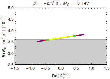
Refer to caption
Refer to caption
Refer to caption
Refer to caption
Figure 5: Correlation 𝓑¯(𝑩𝒔𝝁+𝝁)bold-¯𝓑bold-→subscript𝑩𝒔superscript𝝁superscript𝝁\overline{\mathcal{B}}(B_{s}\to\mu^{+}\mu^{-}) versus 𝐑𝐞(𝐂𝟗NP)𝐑𝐞superscriptsubscript𝐂9NP\rm{Re}(C_{9}^{\text{NP}}) for 𝜷=±𝟏/𝟑𝜷plus-or-minus13\beta=\pm 1/\sqrt{3} and 𝜷=±𝟐/𝟑𝜷plus-or-minus23\beta=\pm 2/\sqrt{3} setting 𝑴𝒁=𝟑𝐓𝐞𝐕subscript𝑴superscript𝒁bold-′3𝐓𝐞𝐕M_{Z^{\prime}}=3\,{\rm TeV} and different values of 𝑪𝑩𝒔subscript𝑪subscript𝑩𝒔C_{B_{s}} with their colour coding in (LABEL:bins). The gray regions show the experimental range 𝓑¯(𝑩𝒔𝝁+𝝁)=(2.9±0.7)𝟏𝟎𝟗bold-¯𝓑bold-→subscript𝑩𝒔superscript𝝁superscript𝝁bold-⋅plus-or-minus2.90.7superscript109\overline{\mathcal{B}}(B_{s}\to\mu^{+}\mu^{-})=(2.9\pm 0.7)\cdot 10^{-9}.


Refer to caption
Refer to caption
Refer to caption
Refer to caption
Figure 6: Correlations 𝑺𝝍ϕsubscript𝑺𝝍bold-italic-ϕS_{\psi\phi} versus 𝓑¯(𝑩𝒔𝝁+𝝁)bold-¯𝓑bold-→subscript𝑩𝒔superscript𝝁superscript𝝁\overline{\mathcal{B}}(B_{s}\to\mu^{+}\mu^{-}) for 𝜷=±𝟏/𝟑𝜷plus-or-minus13\beta=\pm 1/\sqrt{3} and 𝜷=±𝟐/𝟑𝜷plus-or-minus23\beta=\pm 2/\sqrt{3} setting 𝑴𝒁=𝟑𝐓𝐞𝐕subscript𝑴superscript𝒁bold-′3𝐓𝐞𝐕M_{Z^{\prime}}=3\,{\rm TeV} and different values of 𝑪𝑩𝒔subscript𝑪subscript𝑩𝒔C_{B_{s}} with their colour coding in (LABEL:bins). The gray regions show the experimental range for 𝓑¯(𝑩𝒔𝝁+𝝁)bold-¯𝓑bold-→subscript𝑩𝒔superscript𝝁superscript𝝁\overline{\mathcal{B}}(B_{s}\to\mu^{+}\mu^{-}) and 𝑺𝝍ϕsubscript𝑺𝝍bold-italic-ϕS_{\psi\phi}.


Refer to caption
Refer to caption
Refer to caption
Refer to caption
Figure 7: Correlations 𝑺𝝍ϕsubscript𝑺𝝍bold-italic-ϕS_{\psi\phi} versus 𝐑𝐞(𝐂𝟗NP)𝐑𝐞superscriptsubscript𝐂9NP\rm{Re}(C_{9}^{\text{NP}}) for 𝜷=±𝟏/𝟑𝜷plus-or-minus13\beta=\pm 1/\sqrt{3} and 𝜷=±𝟐/𝟑𝜷plus-or-minus23\beta=\pm 2/\sqrt{3} setting 𝑴𝒁=𝟑𝐓𝐞𝐕subscript𝑴superscript𝒁bold-′3𝐓𝐞𝐕M_{Z^{\prime}}=3\,{\rm TeV} and different values of 𝑪𝑩𝒔subscript𝑪subscript𝑩𝒔C_{B_{s}} with their colour coding in (LABEL:bins).


Refer to caption
Refer to caption
Refer to caption
Refer to caption
Figure 8: Correlations 𝐈𝐦(𝐂𝟗NP)𝐈𝐦superscriptsubscript𝐂9NP\rm{Im}(C_{9}^{\text{NP}}) versus 𝐑𝐞(𝐂𝟗NP)𝐑𝐞superscriptsubscript𝐂9NP\rm{Re}(C_{9}^{\text{NP}}) for 𝜷=±𝟏/𝟑𝜷plus-or-minus13\beta=\pm 1/\sqrt{3} and 𝜷=±𝟐/𝟑𝜷plus-or-minus23\beta=\pm 2/\sqrt{3} setting 𝑴𝒁=𝟑𝐓𝐞𝐕subscript𝑴superscript𝒁bold-′3𝐓𝐞𝐕M_{Z^{\prime}}=3\,{\rm TeV} and different values of 𝑪𝑩𝒔subscript𝑪subscript𝑩𝒔C_{B_{s}} with their colour coding in (LABEL:bins).


Refer to caption
Refer to caption
Refer to caption
Refer to caption
Figure 9: 𝐈𝐦(𝐂𝟏𝟎𝐍𝐏)𝐈𝐦superscriptsubscript𝐂10𝐍𝐏\rm{Im}(C_{10}^{\rm NP}) versus 𝐑𝐞(𝐂𝟏𝟎𝐍𝐏)𝐑𝐞superscriptsubscript𝐂10𝐍𝐏\rm{Re}(C_{10}^{\rm NP}) for 𝜷=±𝟏/𝟑𝜷plus-or-minus13\beta=\pm 1/\sqrt{3} and 𝜷=±𝟐/𝟑𝜷plus-or-minus23\beta=\pm 2/\sqrt{3} setting 𝑴𝒁=𝟑𝐓𝐞𝐕subscript𝑴superscript𝒁bold-′3𝐓𝐞𝐕M_{Z^{\prime}}=3\,{\rm TeV} and different values of 𝑪𝑩𝒔subscript𝑪subscript𝑩𝒔C_{B_{s}} with their colour coding in (LABEL:bins).


Refer to caption
Refer to caption
Refer to caption
Refer to caption
Figure 10: 𝐑𝐞(𝐂𝟏𝟎𝐍𝐏)𝐑𝐞superscriptsubscript𝐂10𝐍𝐏\rm{Re}(C_{10}^{\rm NP}) versus 𝐑𝐞(𝐂𝟗𝐍𝐏)𝐑𝐞superscriptsubscript𝐂9𝐍𝐏\rm{Re}(C_{9}^{\rm NP}) for 𝜷=±𝟏/𝟑𝜷plus-or-minus13\beta=\pm 1/\sqrt{3} and 𝜷=±𝟐/𝟑𝜷plus-or-minus23\beta=\pm 2/\sqrt{3} setting 𝑴𝒁=𝟑𝐓𝐞𝐕subscript𝑴superscript𝒁bold-′3𝐓𝐞𝐕M_{Z^{\prime}}=3\,{\rm TeV} and different values of 𝑪𝑩𝒔subscript𝑪subscript𝑩𝒔C_{B_{s}} with their colour coding in (LABEL:bins).


Refer to caption
Refer to caption
Refer to caption
Refer to caption
Figure 11: 𝐈𝐦(𝐂𝟏𝟎𝐍𝐏)𝐈𝐦superscriptsubscript𝐂10𝐍𝐏\rm{Im}(C_{10}^{\rm NP}) versus 𝐈𝐦(𝐂𝟗𝐍𝐏)𝐈𝐦superscriptsubscript𝐂9𝐍𝐏\rm{Im}(C_{9}^{\rm NP}) for 𝜷=±𝟏/𝟑𝜷plus-or-minus13\beta=\pm 1/\sqrt{3} and 𝜷=±𝟐/𝟑𝜷plus-or-minus23\beta=\pm 2/\sqrt{3} setting 𝑴𝒁=𝟑𝐓𝐞𝐕subscript𝑴superscript𝒁bold-′3𝐓𝐞𝐕M_{Z^{\prime}}=3\,{\rm TeV} and different values of 𝑪𝑩𝒔subscript𝑪subscript𝑩𝒔C_{B_{s}} with their colour coding in (LABEL:bins).


Refer to caption
Refer to caption
Refer to caption
Refer to caption
Figure 12: 𝑺𝝁𝝁𝒔superscriptsubscript𝑺𝝁𝝁𝒔S_{\mu\mu}^{s} versus 𝓑¯(𝑩𝒔𝝁+𝝁)bold-¯𝓑bold-→subscript𝑩𝒔superscript𝝁superscript𝝁\overline{\mathcal{B}}(B_{s}\to\mu^{+}\mu^{-}) for 𝜷=±𝟏/𝟑𝜷plus-or-minus13\beta=\pm 1/\sqrt{3} and 𝜷=±𝟐/𝟑𝜷plus-or-minus23\beta=\pm 2/\sqrt{3} setting 𝑴𝒁=𝟑𝐓𝐞𝐕subscript𝑴superscript𝒁bold-′3𝐓𝐞𝐕M_{Z^{\prime}}=3\,{\rm TeV} and different values of 𝑪𝑩𝒔subscript𝑪subscript𝑩𝒔C_{B_{s}} with their colour coding in (LABEL:bins). The gray regions show the experimental range for 𝓑¯(𝑩𝒔𝝁+𝝁)bold-¯𝓑bold-→subscript𝑩𝒔superscript𝝁superscript𝝁\overline{\mathcal{B}}(B_{s}\to\mu^{+}\mu^{-}).


In Fig. 5 we show 𝓑¯(𝑩𝒔𝝁+𝝁)bold-¯𝓑bold-→subscript𝑩𝒔superscript𝝁superscript𝝁\overline{\mathcal{B}}(B_{s}\to\mu^{+}\mu^{-}) versus 𝐑𝐞(𝐂𝟗NP)𝐑𝐞superscriptsubscript𝐂9NP\rm{Re}(C_{9}^{\text{NP}}) for the four models considered. These four plots exhibit the structure identified through the ratio 𝑹𝟏subscript𝑹1R_{1} in (28) for which numerical values have been given in Table 2. In particular we observe the following features666We do not show the SM point in the plots as it corresponds to the point where various curves cross each other and in any case for coefficients that vanish in the SM it is obvious where the SM point is placed in the plot.:

  • For a given 𝑪𝑩𝒔𝟏subscript𝑪subscript𝑩𝒔1C_{B_{s}}\not=1, one can always find an oasis in which 𝐑𝐞(𝐂𝟗NP)𝐑𝐞superscriptsubscript𝐂9NP\rm{Re}(C_{9}^{\text{NP}}) is negative softening significantly the 𝑩𝒅𝑲𝝁+𝝁bold-→subscript𝑩𝒅superscript𝑲superscript𝝁superscript𝝁B_{d}\to K^{*}\mu^{+}\mu^{-} anomalies. However while for 𝜷=𝟐/𝟑𝜷23\beta=-2/\sqrt{3} and 𝜷=𝟏/𝟑𝜷13\beta=-1/\sqrt{3} the values 𝐑𝐞(𝐂𝟗NP)=0.8𝐑𝐞superscriptsubscript𝐂9NP0.8\rm{Re}(C_{9}^{\text{NP}})=-0.8 and 𝐑𝐞(𝐂𝟗NP)=0.4𝐑𝐞superscriptsubscript𝐂9NP0.4\rm{Re}(C_{9}^{\text{NP}})=-0.4 can be reached respectively, this is not possible for models with 𝜷>𝟎𝜷0\beta>0.

  • For 𝜷<𝟎𝜷0\beta<0 the branching ratio 𝓑¯(𝑩𝒔𝝁+𝝁)bold-¯𝓑bold-→subscript𝑩𝒔superscript𝝁superscript𝝁\overline{\mathcal{B}}(B_{s}\to\mu^{+}\mu^{-}) remains SM-like although in accordance with the relation (28) it is suppressed relative to its SM value for negative 𝐑𝐞(𝐂𝟗NP)𝐑𝐞superscriptsubscript𝐂9NP\rm{Re}(C_{9}^{\text{NP}}). For the largest values of 𝑪𝑩𝒔subscript𝑪subscript𝑩𝒔C_{B_{s}} (purple and blue lines) this suppression can reach for most negative values of 𝐑𝐞(𝐂𝟗NP)𝐑𝐞superscriptsubscript𝐂9NP\rm{Re}(C_{9}^{\text{NP}}) 𝟒%percent44\% and 𝟕%percent77\% for 𝜷=𝟐/𝟑𝜷23\beta=-2/\sqrt{3} and 𝜷=𝟏/𝟑𝜷13\beta=-1/\sqrt{3}, respectively. The slope of the strict correlation between these two observables depends on 𝜷𝜷\beta. This correlation is presently supported by the data for both observables even if the effects in 𝓑¯(𝑩𝒔𝝁+𝝁)bold-¯𝓑bold-→subscript𝑩𝒔superscript𝝁superscript𝝁\overline{\mathcal{B}}(B_{s}\to\mu^{+}\mu^{-}) are small.

  • Looking at these four plots simultaneously we note that going from negative to positive values of 𝜷𝜷\beta the correlation line moves counter clock-wise with the center of the clock placed at the SM value. This of course means that with increasing beta the correlation 𝓑¯(𝑩𝒔𝝁+𝝁)bold-¯𝓑bold-→subscript𝑩𝒔superscript𝝁superscript𝝁\overline{\mathcal{B}}(B_{s}\to\mu^{+}\mu^{-}) versus 𝐑𝐞(𝐂𝟗NP)𝐑𝐞superscriptsubscript𝐂9NP\rm{Re}(C_{9}^{\text{NP}}) observed for 𝜷<𝟎𝜷0\beta<0 changes into anti-correlation for 𝜷>𝟎𝜷0\beta>0, which is rather pronounced in the case of 𝜷=𝟐/𝟑𝜷23\beta=2/\sqrt{3}. Consequently the suppression of 𝓑¯(𝑩𝒔𝝁+𝝁)bold-¯𝓑bold-→subscript𝑩𝒔superscript𝝁superscript𝝁\overline{\mathcal{B}}(B_{s}\to\mu^{+}\mu^{-}) implies positive values of 𝐑𝐞(𝐂𝟗NP)𝐑𝐞superscriptsubscript𝐂9NP\rm{Re}(C_{9}^{\text{NP}}) which is not what we want to understand 𝑩𝒅𝑲𝝁+𝝁bold-→subscript𝑩𝒅superscript𝑲superscript𝝁superscript𝝁B_{d}\to K^{*}\mu^{+}\mu^{-} data. We also note that for 𝜷>𝟎𝜷0\beta>0 𝐑𝐞(𝐂𝟗NP)𝐑𝐞superscriptsubscript𝐂9NP\rm{Re}(C_{9}^{\text{NP}}) remains small but the effects in 𝓑¯(𝑩𝒔𝝁+𝝁)bold-¯𝓑bold-→subscript𝑩𝒔superscript𝝁superscript𝝁\overline{\mathcal{B}}(B_{s}\to\mu^{+}\mu^{-}) can be larger than for 𝜷<𝟎𝜷0\beta<0. These scenarios would be the favorite ones if the 𝑩𝒅𝑲𝝁+𝝁bold-→subscript𝑩𝒅superscript𝑲superscript𝝁superscript𝝁B_{d}\to K^{*}\mu^{+}\mu^{-} anomalies decreased or disappeared in the future while the experimental branching ratio 𝓑¯(𝑩𝒔𝝁+𝝁)bold-¯𝓑bold-→subscript𝑩𝒔superscript𝝁superscript𝝁\overline{\mathcal{B}}(B_{s}\to\mu^{+}\mu^{-}) turned out to be indeed by 𝟐𝟎%percent2020\% suppressed below its SM value as present central experimental and SM values seem to indicate. In this case the model with 𝜷=𝟏/𝟑𝜷13\beta=1/\sqrt{3} would be the winner.

This pattern of effects for negative and positive values of 𝜷𝜷\beta is also seen in Figs. 6 and 7 where we show the correlations between 𝑺𝝍ϕsubscript𝑺𝝍bold-italic-ϕS_{\psi\phi} versus 𝓑¯(𝑩𝒔𝝁+𝝁)bold-¯𝓑bold-→subscript𝑩𝒔superscript𝝁superscript𝝁\overline{\mathcal{B}}(B_{s}\to\mu^{+}\mu^{-}) and 𝑺𝝍ϕsubscript𝑺𝝍bold-italic-ϕS_{\psi\phi} versus 𝐑𝐞(𝐂𝟗NP)𝐑𝐞superscriptsubscript𝐂9NP\rm{Re}(C_{9}^{\text{NP}}), respectively. In particular we find that for models with 𝜷<𝟎𝜷0\beta<0 for most negative values of 𝐑𝐞(𝐂𝟗NP)𝐑𝐞superscriptsubscript𝐂9NP\rm{Re}(C_{9}^{\text{NP}}) and smallest values of 𝓑¯(𝑩𝒔𝝁+𝝁)bold-¯𝓑bold-→subscript𝑩𝒔superscript𝝁superscript𝝁\overline{\mathcal{B}}(B_{s}\to\mu^{+}\mu^{-}) the negative values of 𝑺𝝍ϕsubscript𝑺𝝍bold-italic-ϕS_{\psi\phi} are favoured. But as the values of 𝑺𝝍ϕsubscript𝑺𝝍bold-italic-ϕS_{\psi\phi} are rather sensitive for a given value of 𝑪𝑩𝒔subscript𝑪subscript𝑩𝒔C_{B_{s}} to the value of 𝓑¯(𝑩𝒔𝝁+𝝁)bold-¯𝓑bold-→subscript𝑩𝒔superscript𝝁superscript𝝁\overline{\mathcal{B}}(B_{s}\to\mu^{+}\mu^{-}), away from the lower bound on this branching ratio also positive values of 𝑺𝝍ϕsubscript𝑺𝝍bold-italic-ϕS_{\psi\phi} are allowed. This is in particular the case for largest values of 𝑪𝑩𝒔subscript𝑪subscript𝑩𝒔C_{B_{s}}.

Bearing this ambiguity in mind, we identify therefore for a given 𝑪𝑩𝒔subscript𝑪subscript𝑩𝒔C_{B_{s}} a triple correlation between 𝐑𝐞(𝐂𝟗NP)𝐑𝐞superscriptsubscript𝐂9NP\rm{Re}(C_{9}^{\text{NP}}), 𝓑¯(𝑩𝒔𝝁+𝝁)bold-¯𝓑bold-→subscript𝑩𝒔superscript𝝁superscript𝝁\overline{\mathcal{B}}(B_{s}\to\mu^{+}\mu^{-}) and 𝑺𝝍ϕsubscript𝑺𝝍bold-italic-ϕS_{\psi\phi} that is an important test of this model. Interestingly the requirement of a most negative 𝐑𝐞(𝐂𝟗NP)𝐑𝐞superscriptsubscript𝐂9NP\rm{Re}(C_{9}^{\text{NP}}) shifts automatically the other two observables closer to the data.

While the departure of 𝑺𝝍ϕsubscript𝑺𝝍bold-italic-ϕS_{\psi\phi} from its SM value is already a clear signal of new sources of CP-violation in 𝚫𝑭=𝟐𝚫𝑭2\Delta F=2 transitions, non-vanishing imaginary parts of 𝑪𝟗subscript𝑪9C_{9} and 𝑪𝟏𝟎subscript𝑪10C_{10} are signals of such new effects in 𝚫𝑭=𝟏𝚫𝑭1\Delta F=1 transitions. In Figs. 8 and 9 we show the correlations 𝐈𝐦(𝐂𝟗NP)𝐈𝐦superscriptsubscript𝐂9NP\rm{Im}(C_{9}^{\text{NP}}) versus 𝐑𝐞(𝐂𝟗NP)𝐑𝐞superscriptsubscript𝐂9NP\rm{Re}(C_{9}^{\text{NP}}) and 𝐈𝐦(𝐂𝟏𝟎NP)𝐈𝐦superscriptsubscript𝐂10NP\rm{Im}(C_{10}^{\text{NP}}) versus 𝐑𝐞(𝐂𝟏𝟎NP)𝐑𝐞superscriptsubscript𝐂10NP\rm{Re}(C_{10}^{\text{NP}}), respectively. The fact that the pattern in both figures for a given 𝜷𝜷\beta is the same, even if the size of NP effects differs, is related to the relation (29).

We again observe that for 𝜷<𝟎𝜷0\beta<0 NP effects are mainly seen in 𝐈𝐦(𝐂𝟗𝐍𝐏)𝐈𝐦superscriptsubscript𝐂9𝐍𝐏\rm{Im}(C_{9}^{\rm NP}) while for 𝜷>𝟎𝜷0\beta>0 in 𝐈𝐦(𝐂𝟏𝟎𝐍𝐏)𝐈𝐦superscriptsubscript𝐂10𝐍𝐏\rm{Im}(C_{10}^{\rm NP}). In particular for 𝜷=𝟏/𝟑𝜷13\beta=1/\sqrt{3} NP effects in 𝑪𝟗subscript𝑪9C_{9} practically vanish which is a good test of this model. Dependently on the values of 𝑪𝑩𝒔subscript𝑪subscript𝑩𝒔C_{B_{s}} and |𝜷|𝜷|\beta|, the CP-asymmetry 𝑨𝟖delimited-⟨⟩subscript𝑨8\langle A_{8}\rangle could reach (𝟐𝟑)%percent23(2-3)\% and the asymmetry 𝑨𝟕delimited-⟨⟩subscript𝑨7\langle A_{7}\rangle even (𝟑𝟒)%percent34(3-4)\% for 𝜷<𝟎𝜷0\beta<0 and 𝜷>𝟎𝜷0\beta>0, respectively.

Finally in Figs. 10 and 11 we show the correlations 𝐑𝐞(𝐂𝟏𝟎𝐍𝐏)𝐑𝐞superscriptsubscript𝐂10𝐍𝐏\rm{Re}(C_{10}^{\rm NP}) versus 𝐑𝐞(𝐂𝟗𝐍𝐏)𝐑𝐞superscriptsubscript𝐂9𝐍𝐏\rm{Re}(C_{9}^{\rm NP}) and 𝐈𝐦(𝐂𝟏𝟎𝐍𝐏)𝐈𝐦superscriptsubscript𝐂10𝐍𝐏\rm{Im}(C_{10}^{\rm NP}) versus 𝐈𝐦(𝐂𝟗𝐍𝐏)𝐈𝐦superscriptsubscript𝐂9𝐍𝐏\rm{Im}(C_{9}^{\rm NP}) for the four 331 models considered by us. These results follow from (28).

New sources of CP-violation can also be tested in 𝑩𝒔𝝁+𝝁bold-→subscript𝑩𝒔superscript𝝁superscript𝝁B_{s}\to\mu^{+}\mu^{-} through the asymmetry 𝑺𝝁𝝁subscript𝑺𝝁𝝁S_{\mu\mu} defined in (58) and studied in detail in [19, 44] in the context of general 𝒁superscript𝒁bold-′Z^{\prime} models. In Fig. 12 we show the correlation of 𝑺𝝁𝝁𝒔superscriptsubscript𝑺𝝁𝝁𝒔S_{\mu\mu}^{s} versus 𝓑¯(𝑩𝒔𝝁+𝝁)bold-¯𝓑bold-→subscript𝑩𝒔superscript𝝁superscript𝝁\overline{\mathcal{B}}(B_{s}\to\mu^{+}\mu^{-}) in 331 model considered. As expected the effects in the models with 𝜷>𝟎𝜷0\beta>0 are larger than for 𝜷<𝟎𝜷0\beta<0. Similar to the case of 𝑺𝝍ϕsubscript𝑺𝝍bold-italic-ϕS_{\psi\phi} the required suppression of 𝓑¯(𝑩𝒔𝝁+𝝁)bold-¯𝓑bold-→subscript𝑩𝒔superscript𝝁superscript𝝁\overline{\mathcal{B}}(B_{s}\to\mu^{+}\mu^{-}) favours negative values of 𝑺𝝁𝝁𝒔subscriptsuperscript𝑺𝒔𝝁𝝁S^{s}_{\mu\mu} in all models.

As stressed in [11] the Wilson coefficient 𝑪𝟗𝐍𝐏superscriptsubscript𝑪9𝐍𝐏C_{9}^{\rm NP} by itself has difficulty in removing completely the anomalies in 𝑩𝒅𝑲𝝁+𝝁bold-→subscript𝑩𝒅superscript𝑲superscript𝝁superscript𝝁B_{d}\to K^{*}\mu^{+}\mu^{-} due to the constraint from 𝑩𝒅𝑲𝝁+𝝁bold-→subscript𝑩𝒅𝑲superscript𝝁superscript𝝁B_{d}\to K\mu^{+}\mu^{-}. We have seen that even without this constraint the values of 𝐑𝐞𝐂𝟗𝐍𝐏𝐑𝐞superscriptsubscript𝐂9𝐍𝐏\rm{Re}~{}C_{9}^{\rm NP} have to be larger than 0.80.8-0.8 but this could turn out to be sufficient to reproduce the data when they improve. Still it is of interest to have a closer look at 𝑩𝒅𝑲𝝁+𝝁bold-→subscript𝑩𝒅𝑲superscript𝝁superscript𝝁B_{d}\to K\mu^{+}\mu^{-} within the four 331 models analysed by us.

To this end the approximate formula for the branching ratio confined to large 𝒒𝟐superscript𝒒2q^{2} region by the authors of [11] is very useful. Lattice calculations of the relevant form factors are making significant progress here [68, 69] and the importance of this decay will increase in the future. Neglecting the interference between NP contributions the formula of [11] reduces in 331 models to

𝟏𝟎𝟕×𝓑(𝑩𝒅𝑲𝝁+𝝁)[14.2,𝟐𝟐]=1.11+0.27𝐑𝐞(𝐂𝟗NP)(𝟏𝟏𝐑𝟏),superscript107𝓑subscriptbold-→subscript𝑩𝒅𝑲superscript𝝁superscript𝝁14.2221.110.27𝐑𝐞superscriptsubscript𝐂9NP11subscript𝐑110^{7}\times\mathcal{B}(B_{d}\to K\mu^{+}\mu^{-})_{[14.2,22]}=1.11+0.27~{}\rm{Re}(C_{9}^{\text{NP}})\left(1-\frac{1}{R_{1}}\right), (76)

where we have used (28) to express 𝐑𝐞(𝐂𝟏𝟎NP)𝐑𝐞superscriptsubscript𝐂10NP\rm{Re}(C_{10}^{\text{NP}}) in terms of 𝐑𝐞(𝐂𝟗NP)𝐑𝐞superscriptsubscript𝐂9NP\rm{Re}(C_{9}^{\text{NP}}). The error on the first SM term is estimated to be 𝟏𝟎%percent1010\% [68, 69]. This should be compared with the LHCb result

𝟏𝟎𝟕×𝓑(𝑩𝒅𝑲𝝁+𝝁)[14.2,𝟐𝟐]=1.04±0.12(𝐋𝐇𝐂𝐛).superscript107𝓑subscriptbold-→subscript𝑩𝒅𝑲superscript𝝁superscript𝝁14.222plus-or-minus1.040.12𝐋𝐇𝐂𝐛10^{7}\times\mathcal{B}(B_{d}\to K\mu^{+}\mu^{-})_{[14.2,22]}=1.04\pm 0.12\qquad{(\rm LHCb).} (77)

Using (76) we show in Fig. 13 the correlation between 𝓑(𝑩𝒅𝑲𝝁+𝝁)[14.2,𝟐𝟐]𝓑subscriptbold-→subscript𝑩𝒅𝑲superscript𝝁superscript𝝁14.222\mathcal{B}(B_{d}\to K\mu^{+}\mu^{-})_{[14.2,22]} and 𝐑𝐞(𝐂𝟗NP)𝐑𝐞superscriptsubscript𝐂9NP\rm{Re}(C_{9}^{\text{NP}}) for the four 331 models in question.

Refer to caption
Refer to caption
Refer to caption
Refer to caption
Figure 13: Correlation 𝓑(𝑩𝒅𝑲𝝁+𝝁)[14.2,𝟐𝟐]𝓑subscriptbold-→subscript𝑩𝒅𝑲superscript𝝁superscript𝝁14.222\mathcal{B}(B_{d}\to K\mu^{+}\mu^{-})_{[14.2,22]} versus 𝐑𝐞(𝐂𝟗𝐍𝐏)𝐑𝐞superscriptsubscript𝐂9𝐍𝐏\rm{Re}(C_{9}^{\rm NP}) for 𝜷=±𝟏/𝟑𝜷plus-or-minus13\beta=\pm 1/\sqrt{3} and 𝜷=±𝟐/𝟑𝜷plus-or-minus23\beta=\pm 2/\sqrt{3} setting 𝑴𝒁=𝟑𝐓𝐞𝐕subscript𝑴superscript𝒁bold-′3𝐓𝐞𝐕M_{Z^{\prime}}=3\,{\rm TeV}, 𝓑¯(𝑩𝒔𝝁+𝝁)𝓑¯(𝑩𝒔𝝁+𝝁)SMbold-¯𝓑bold-→subscript𝑩𝒔superscript𝝁superscript𝝁bold-¯𝓑subscriptbold-→subscript𝑩𝒔superscript𝝁superscript𝝁SM\overline{\mathcal{B}}(B_{s}\to\mu^{+}\mu^{-})\leq\overline{\mathcal{B}}(B_{s}\to\mu^{+}\mu^{-})_{\text{SM}} (black) and 𝓑¯(𝑩𝒔𝝁+𝝁)𝓑¯(𝑩𝒔𝝁+𝝁)SMbold-¯𝓑bold-→subscript𝑩𝒔superscript𝝁superscript𝝁bold-¯𝓑subscriptbold-→subscript𝑩𝒔superscript𝝁superscript𝝁SM\overline{\mathcal{B}}(B_{s}\to\mu^{+}\mu^{-})\geq\overline{\mathcal{B}}(B_{s}\to\mu^{+}\mu^{-})_{\text{SM}} (yellow) . The gray regions show the experimental range for 𝓑(𝑩𝒅𝑲𝝁+𝝁)[14.2,𝟐𝟐]𝓑subscriptbold-→subscript𝑩𝒅𝑲superscript𝝁superscript𝝁14.222\mathcal{B}(B_{d}\to K\mu^{+}\mu^{-})_{[14.2,22]} in (77).


We observe that the pattern of the correlations is similar to the ones in Fig 5 which originates in the fact that 𝓑(𝑩𝒅𝑲𝝁+𝝁)[14.2,𝟐𝟐]𝓑subscriptbold-→subscript𝑩𝒅𝑲superscript𝝁superscript𝝁14.222\mathcal{B}(B_{d}\to K\mu^{+}\mu^{-})_{[14.2,22]} is strongly correlated with 𝓑¯(𝑩𝒔𝝁+𝝁)bold-¯𝓑bold-→subscript𝑩𝒔superscript𝝁superscript𝝁\overline{\mathcal{B}}(B_{s}\to\mu^{+}\mu^{-}) within LHS models as already shown in [13] for a general LHS model. Moreover, as 𝑹𝟏subscript𝑹1R_{1} is fixed in a given model and its values have been collected in Table 2 the straight lines in Fig 5 can be easily understood.

There are two messages from this exercise:

  • Our results for 𝐑𝐞(𝐂𝟗𝐍𝐏)𝐑𝐞superscriptsubscript𝐂9𝐍𝐏\rm{Re}(C_{9}^{\rm NP}) are fully in accordance with the present data on 𝓑(𝑩𝒅𝑲𝝁+𝝁)[14.2,𝟐𝟐]𝓑subscriptbold-→subscript𝑩𝒅𝑲superscript𝝁superscript𝝁14.222\mathcal{B}(B_{d}\to K\mu^{+}\mu^{-})_{[14.2,22]}.

  • On the basis of Figs. 5 and 13 there is a triple correlation between 𝓑(𝑩𝒅𝑲𝝁+𝝁)[14.2,𝟐𝟐]𝓑subscriptbold-→subscript𝑩𝒅𝑲superscript𝝁superscript𝝁14.222\mathcal{B}(B_{d}\to K\mu^{+}\mu^{-})_{[14.2,22]}, 𝐑𝐞(𝐂𝟗𝐍𝐏)𝐑𝐞superscriptsubscript𝐂9𝐍𝐏\rm{Re}(C_{9}^{\rm NP}) and 𝓑¯(𝑩𝒔𝝁+𝝁)bold-¯𝓑bold-→subscript𝑩𝒔superscript𝝁superscript𝝁\overline{\mathcal{B}}(B_{s}\to\mu^{+}\mu^{-}) which constitutes an important test for the models in question. We indicate this correlation in Fig. 13 by showing when the latter branching ratio is suppressed (black) or enhanced (yellow) with respect to its SM value in accordance with the colour coding in DNA-charts of [1].

6.3 Non-CMFV case (𝑩𝒅subscript𝑩𝒅B_{d}-system)

We have seen in the case of the MFV limit that 𝓑(𝑩𝒅𝝁+𝝁)𝓑bold-→subscript𝑩𝒅superscript𝝁superscript𝝁{\mathcal{B}}(B_{d}\to\mu^{+}\mu^{-}) is predicted to be suppressed relative to its SM value when 𝐑𝐞(𝐂𝟗NP)𝐑𝐞superscriptsubscript𝐂9NP\rm{Re}(C_{9}^{\text{NP}}) is negative. This moves the theory away from the central value of the experimental branching ratio. However, in the non-MFV case we can choose the particular oasis in the space (𝒔~𝟏𝟑,𝜹𝟏)subscriptbold-~𝒔13subscript𝜹1(\tilde{s}_{13},\delta_{1}) in which 𝓑(𝑩𝒅𝝁+𝝁)𝓑bold-→subscript𝑩𝒅superscript𝝁superscript𝝁{\mathcal{B}}(B_{d}\to\mu^{+}\mu^{-}) is enhanced.

In the left upper panel of Fig. 14 we show 𝓑(𝑩𝒅𝝁+𝝁)𝓑bold-→subscript𝑩𝒅superscript𝝁superscript𝝁{\mathcal{B}}(B_{d}\to\mu^{+}\mu^{-}) versus 𝑺𝝍𝑲𝑺subscript𝑺𝝍subscript𝑲𝑺S_{\psi K_{S}} again for 𝜷=𝟐/𝟑𝜷23\beta=-2/\sqrt{3} and different bins of 𝑪𝑩𝒅subscript𝑪subscript𝑩𝒅C_{B_{d}}. We observe that the values of 𝓑(𝑩𝒅𝝁+𝝁)𝓑bold-→subscript𝑩𝒅superscript𝝁superscript𝝁{\mathcal{B}}(B_{d}\to\mu^{+}\mu^{-}) are SM-like and as already expected from the values of 𝚫𝑨𝝁𝝁¯superscriptsubscript𝚫𝑨𝝁bold-¯𝝁\Delta_{A}^{\mu\bar{\mu}} the central experimental value of this branching ratio cannot be reproduced in this model.

More interesting results are found for 𝜷>𝟎𝜷0\beta>0. In the right upper panel of Fig. 14 we show 𝓑(𝑩𝒅𝝁+𝝁)𝓑bold-→subscript𝑩𝒅superscript𝝁superscript𝝁{\mathcal{B}}(B_{d}\to\mu^{+}\mu^{-}) versus 𝑺𝝍𝑲𝑺subscript𝑺𝝍subscript𝑲𝑺S_{\psi K_{S}} for 𝜷=𝟐/𝟑𝜷23\beta=2/\sqrt{3}. We observe that now enhancement of 𝓑(𝑩𝒅𝝁+𝝁)𝓑bold-→subscript𝑩𝒅superscript𝝁superscript𝝁{\mathcal{B}}(B_{d}\to\mu^{+}\mu^{-}) can reach 𝟐𝟎%percent2020\% over its SM value but still far away from the central experimental value. For 𝜷=𝟏/𝟑𝜷13\beta=-1/\sqrt{3} and 𝜷=𝟏/𝟑𝜷13\beta=1/\sqrt{3} NP effects turn out to be larger and smaller relative to 𝜷=𝟐/𝟑𝜷minus-or-plus23\beta=\mp 2/\sqrt{3} respectively, as one could deduce from the values of the axial-vector couplings.
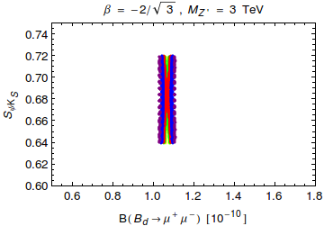
Refer to caption
Refer to caption
Refer to caption
Refer to caption
Figure 14: Correlation 𝓑(𝑩𝒅𝝁+𝝁)𝓑bold-→subscript𝑩𝒅superscript𝝁superscript𝝁{\mathcal{B}}(B_{d}\to\mu^{+}\mu^{-}) versus 𝑺𝝍𝑲𝑺subscript𝑺𝝍subscript𝑲𝑺S_{\psi K_{S}} for 𝜷=±𝟏/𝟑𝜷plus-or-minus13\beta=\pm 1/\sqrt{3} and 𝜷=±𝟐/𝟑𝜷plus-or-minus23\beta=\pm 2/\sqrt{3} setting 𝑴𝒁=𝟑𝐓𝐞𝐕subscript𝑴superscript𝒁bold-′3𝐓𝐞𝐕M_{Z^{\prime}}=3\,{\rm TeV} and different values of 𝑪𝑩𝒔subscript𝑪subscript𝑩𝒔C_{B_{s}} with their colour coding in (LABEL:bins).


Next in Fig. 15 we show 𝓑(𝑩𝒅𝝁+𝝁)𝓑bold-→subscript𝑩𝒅superscript𝝁superscript𝝁{\mathcal{B}}(B_{d}\to\mu^{+}\mu^{-}) versus 𝓑¯(𝑩𝒔𝝁+𝝁)bold-¯𝓑bold-→subscript𝑩𝒔superscript𝝁superscript𝝁\overline{\mathcal{B}}(B_{s}\to\mu^{+}\mu^{-}) for the four models considered with the colour coding for 𝜷𝜷\beta given in (75). We also show the CMFV line. As the uncertainty in the latter line should be reduced to a few percent in this decade, this plot could turn out to be useful for testing and distinguishing the four 331 models.
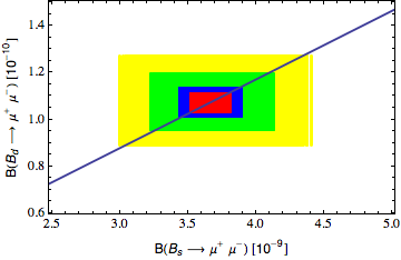
Refer to caption
Figure 15: Correlation 𝓑(𝑩𝒅𝝁+𝝁)𝓑bold-→subscript𝑩𝒅superscript𝝁superscript𝝁{\mathcal{B}}(B_{d}\to\mu^{+}\mu^{-}) versus 𝓑¯(𝑩𝒔𝝁+𝝁)bold-¯𝓑bold-→subscript𝑩𝒔superscript𝝁superscript𝝁\overline{\mathcal{B}}(B_{s}\to\mu^{+}\mu^{-}) for the four models considered in the paper. The colour coding for 𝜷𝜷\beta is given in (75). The straight line represents CMFV.


6.4 Non-CMFV case for 𝒃𝒔𝝂𝝂¯bold-→𝒃𝒔𝝂bold-¯𝝂b\to s\nu\bar{\nu}, 𝑲+𝝅+𝝂𝝂¯bold-→superscript𝑲superscript𝝅𝝂bold-¯𝝂K^{+}\rightarrow\pi^{+}\nu\bar{\nu} and 𝑲𝑳𝝅𝟎𝝂𝝂¯bold-→subscript𝑲𝑳superscript𝝅0𝝂bold-¯𝝂K_{L}\rightarrow\pi^{0}\nu\bar{\nu}

6.4.1 Preliminaries

Finally, we turn our discussion to decays with neutrinos in the final state. We recall that for given 𝜷𝜷\beta, 𝑪𝑩𝒅subscript𝑪subscript𝑩𝒅C_{B_{d}}, 𝑪𝑩𝒔subscript𝑪subscript𝑩𝒔C_{B_{s}} and the chosen oases in 𝑩𝒅subscript𝑩𝒅B_{d} and 𝑩𝒔subscript𝑩𝒔B_{s} systems the corresponding oasis including its size is fixed so that definite predictions for 𝒃𝒔𝝂𝝂¯bold-→𝒃𝒔𝝂bold-¯𝝂b\to s\nu\bar{\nu} transition, 𝑲+𝝅+𝝂𝝂¯bold-→superscript𝑲superscript𝝅𝝂bold-¯𝝂K^{+}\rightarrow\pi^{+}\nu\bar{\nu} and 𝑲𝑳𝝅𝟎𝝂𝝂¯bold-→subscript𝑲𝑳superscript𝝅0𝝂bold-¯𝝂K_{L}\rightarrow\pi^{0}\nu\bar{\nu} can be made.

The inspection of the correlations presented in Section 4 teaches us about the following facts:

  • NP effects in 𝜺𝑲subscript𝜺𝑲\varepsilon_{K} are small but this is not a problem as with our nominal values of |𝑽𝒖𝒃|subscript𝑽𝒖𝒃|V_{ub}|, |𝑽𝒄𝒃|subscript𝑽𝒄𝒃|V_{cb}| and 𝜸𝜸\gamma SM value of 𝜺𝑲subscript𝜺𝑲\varepsilon_{K} agrees well with the data.

  • For 𝜷>𝟎𝜷0\beta>0 NP effects in these decays are found to be small but are larger in the cases with 𝜷<𝟎𝜷0\beta<0 where 𝒁superscript𝒁bold-′Z^{\prime} couplings to neutrinos are largest.

  • Similarly NP effects in 𝑲+𝝅+𝝂𝝂¯bold-→superscript𝑲superscript𝝅𝝂bold-¯𝝂K^{+}\rightarrow\pi^{+}\nu\bar{\nu} and 𝑲𝑳𝝅𝟎𝝂𝝂¯bold-→subscript𝑲𝑳superscript𝝅0𝝂bold-¯𝝂K_{L}\rightarrow\pi^{0}\nu\bar{\nu} are small as we have already expected on the basis of the relation (37).

6.4.2 The 𝒃𝒔𝝂𝝂¯bold-→𝒃𝒔𝝂bold-¯𝝂b\to s\nu\bar{\nu} transitions

Refer to caption
Refer to caption
Refer to caption
Refer to caption
Figure 16: 𝓑¯(𝑩𝒔𝝁+𝝁)bold-¯𝓑bold-→subscript𝑩𝒔superscript𝝁superscript𝝁\overline{\mathcal{B}}(B_{s}\to\mu^{+}\mu^{-}) versus the ratio in (78) for all four 𝜷=±𝟐𝟑,±𝟏𝟑𝜷plus-or-minus23plus-or-minus13\beta=\pm\frac{2}{\sqrt{3}},\pm\frac{1}{\sqrt{3}}.


In the absence of right-handed currents one finds [70]

𝑹𝝂𝝂¯=𝓑(𝑩𝑲𝝂𝝂¯)𝓑(𝑩𝑲𝝂𝝂¯)𝐒𝐌=𝓑(𝑩𝑲𝝂𝝂¯)𝓑(𝑩𝑲𝝂𝝂¯)𝐒𝐌=𝓑(𝑩𝑿𝒔𝝂𝝂¯)𝓑(𝑩𝑿𝒔𝝂𝝂¯)𝐒𝐌=|𝑿𝐋(𝑩𝒔)|𝟐|𝜼𝑿𝑿𝟎(𝒙𝒕)|𝟐,subscript𝑹𝝂bold-¯𝝂𝓑bold-→𝑩𝑲𝝂bold-¯𝝂𝓑subscriptbold-→𝑩𝑲𝝂bold-¯𝝂𝐒𝐌𝓑bold-→𝑩superscript𝑲𝝂bold-¯𝝂𝓑subscriptbold-→𝑩superscript𝑲𝝂bold-¯𝝂𝐒𝐌𝓑bold-→𝑩subscript𝑿𝒔𝝂bold-¯𝝂𝓑subscriptbold-→𝑩subscript𝑿𝒔𝝂bold-¯𝝂𝐒𝐌superscriptsubscript𝑿𝐋subscript𝑩𝒔2superscriptsubscript𝜼𝑿subscript𝑿0subscript𝒙𝒕2R_{\nu\bar{\nu}}=\frac{\mathcal{B}(B\to K\nu\bar{\nu})}{\mathcal{B}(B\to K\nu\bar{\nu})_{\rm SM}}=\frac{\mathcal{B}(B\to K^{*}\nu\bar{\nu})}{\mathcal{B}(B\to K^{*}\nu\bar{\nu})_{\rm SM}}=\frac{\mathcal{B}(B\to X_{s}\nu\bar{\nu})}{\mathcal{B}(B\to X_{s}\nu\bar{\nu})_{\rm SM}}=\frac{|X_{\rm L}(B_{s})|^{2}}{|\eta_{X}X_{0}(x_{t})|^{2}}~{}, (78)

with

𝑿𝐋(𝑩𝒔)=𝜼𝑿𝑿𝟎(𝒙𝒕)+𝚫𝑿(𝑩𝒔)subscript𝑿𝐋subscript𝑩𝒔subscript𝜼𝑿subscript𝑿0subscript𝒙𝒕𝚫𝑿subscript𝑩𝒔X_{\rm L}(B_{s})=\eta_{X}X_{0}(x_{t})+\Delta X(B_{s}) (79)

and 𝚫𝑿(𝑩𝒔)𝚫𝑿subscript𝑩𝒔\Delta X(B_{s}) given in (24). The QCD factor 𝜼𝑿=0.994subscript𝜼𝑿0.994\eta_{X}=0.994 [71]. In this case the NLO electroweak corrections are of the order of one per mil [51] when similarly to our discussion of 𝜼𝐞𝐟𝐟subscript𝜼𝐞𝐟𝐟\eta_{\rm eff} in the context of 𝑩𝒔,𝒅𝝁+𝝁bold-→subscript𝑩𝒔𝒅superscript𝝁superscript𝝁B_{s,d}\to\mu^{+}\mu^{-} decays one uses the normalization of effective Hamiltonian in [50] and the top quark mass is evaluated in the 𝐌𝐒¯bold-¯𝐌𝐒\overline{\rm MS} scheme for QCD and on-shell with respect to electroweak interactions. Thus accidentally 𝜼𝐞𝐟𝐟subscript𝜼𝐞𝐟𝐟\eta_{\rm eff} that includes both QCD and electroweak corrections turns out in this scheme to be practically the same for 𝑲𝝅𝝂𝝂¯bold-→𝑲𝝅𝝂bold-¯𝝂K\to\pi\nu\bar{\nu} and 𝑩𝒔,𝒅𝝁+𝝁bold-→subscript𝑩𝒔𝒅superscript𝝁superscript𝝁B_{s,d}\to\mu^{+}\mu^{-} decays.

The equality of these three ratios is an important test of any LHS scenario. The violation of them would imply the presence of right-handed couplings at work [72, 73, 70]. In the context of 𝒁superscript𝒁bold-′Z^{\prime} models this is clearly seen in Fig. 20 of [19].

The 𝑺𝑼(𝟐)𝑳𝑺𝑼subscript2𝑳SU(2)_{L} relation in (4) satisfied in any LHS model, therefore also in the 331 models presented by us, implies a correlation between 𝑹𝝂𝝂¯subscript𝑹𝝂bold-¯𝝂R_{\nu\bar{\nu}}, 𝓑¯(𝑩𝒔𝝁+𝝁)bold-¯𝓑bold-→subscript𝑩𝒔superscript𝝁superscript𝝁\overline{\mathcal{B}}(B_{s}\to\mu^{+}\mu^{-}) and 𝑪𝟗𝐍𝐏superscriptsubscript𝑪9𝐍𝐏C_{9}^{\rm NP} as shown for a general LHS model in Fig. 9 of [13].

In Fig. 16 we show one of these ratios versus 𝓑¯(𝑩𝒔𝝁+𝝁)bold-¯𝓑bold-→subscript𝑩𝒔superscript𝝁superscript𝝁\overline{\mathcal{B}}(B_{s}\to\mu^{+}\mu^{-}) for the models considered. We observe that in all models considered we have an anti-correlation between these two observables. But the predicted NP effects in all models are rather small. The same conclusion has been reached for general LHS models in [11, 13].
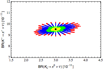
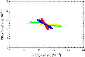
Refer to caption
Refer to caption
Figure 17: Correlations between rare 𝑲𝑲K decays for different values of 𝜷𝜷\beta using the colour coding in (75).


6.4.3 𝑲+𝝅+𝝂𝝂¯bold-→superscript𝑲superscript𝝅𝝂bold-¯𝝂K^{+}\rightarrow\pi^{+}\nu\bar{\nu}, 𝑲𝑳𝝅𝟎𝝂𝝂¯bold-→subscript𝑲𝑳superscript𝝅0𝝂bold-¯𝝂K_{L}\rightarrow\pi^{0}\nu\bar{\nu} and 𝑲𝑳𝝁+𝝁bold-→subscript𝑲𝑳superscript𝝁superscript𝝁K_{L}\to\mu^{+}\mu^{-} decays

The formulae for these decays have been given in [19] and will not be repeated here. In Fig. 17 we show the correlation between 𝓑(𝑲+𝝅+𝝂𝝂¯)𝓑bold-→superscript𝑲superscript𝝅𝝂bold-¯𝝂\mathcal{B}(K^{+}\rightarrow\pi^{+}\nu\bar{\nu}) and 𝓑(𝑲𝑳𝝅𝟎𝝂𝝂¯)𝓑bold-→subscript𝑲𝑳superscript𝝅0𝝂bold-¯𝝂\mathcal{B}(K_{L}\rightarrow\pi^{0}\nu\bar{\nu}) and the one between 𝓑(𝑲+𝝅+𝝂𝝂¯)𝓑bold-→superscript𝑲superscript𝝅𝝂bold-¯𝝂\mathcal{B}(K^{+}\rightarrow\pi^{+}\nu\bar{\nu}) and 𝓑(𝑲𝑳𝝁+𝝁)𝓑bold-→subscript𝑲𝑳superscript𝝁superscript𝝁\mathcal{B}(K_{L}\to\mu^{+}\mu^{-}) for the four models considered. The effects are rather small. What is interesting are the SM values in the middle of both plots that are enhanced over the usual values quoted as a consequence of inclusive value of |𝑽𝒄𝒃|subscript𝑽𝒄𝒃|V_{cb}| used by us.

7 Low and high energy constraints

7.1 Low energy precision observables

Low energy precision observables provide additional bounds on the parameters of the models considered, in particular on the allowed range of 𝑴𝒁subscript𝑴superscript𝒁bold-′M_{Z^{\prime}} as investigated recently in the context of 𝜷=𝟑𝜷3\beta=-\sqrt{3} model in [14]. We want to add that in concrete models studied here the signs of deviations from SM predictions for these observables are fixed providing additional tests beyond the lower bounds on 𝑴𝒁subscript𝑴superscript𝒁bold-′M_{Z^{\prime}}. In what follows we will present the predictions for three such observables, considered also in [14], separately in each model from which the lower bounds on 𝑴𝒁subscript𝑴superscript𝒁bold-′M_{Z^{\prime}} follow.

We begin with the effect due to a 𝒁superscript𝒁bold-′Z^{\prime} gauge boson on the weak charge of a nucleus consisting of 𝒁𝒁Z protons and 𝑵𝑵N neutrons calculated in [74]. In translating this result into our notation one should note that the vector and axial-vector couplings 𝒇𝑽,𝑨subscript𝒇𝑽𝑨f_{V,A} defined in [74] are not equal to our couplings 𝚫𝑽,𝑨(𝒁)subscript𝚫𝑽𝑨superscript𝒁bold-′\Delta_{V,A}(Z^{\prime}) but are related through

𝒇𝑽=𝚫𝑽(𝒁)𝟐,𝒇𝑨=𝚫𝑨(𝒁)𝟐.formulae-sequencesubscript𝒇𝑽subscript𝚫𝑽superscript𝒁bold-′2subscript𝒇𝑨subscript𝚫𝑨superscript𝒁bold-′2f_{V}=\frac{\Delta_{V}(Z^{\prime})}{2},\qquad f_{A}=-\frac{\Delta_{A}(Z^{\prime})}{2}. (80)

We find then (𝚫𝑨𝒆𝒆¯(𝒁)=𝚫𝑨𝝁𝝁¯(𝒁)superscriptsubscript𝚫𝑨𝒆bold-¯𝒆superscript𝒁bold-′superscriptsubscript𝚫𝑨𝝁bold-¯𝝁superscript𝒁bold-′\Delta_{A}^{e\bar{e}}(Z^{\prime})=\Delta_{A}^{\mu\bar{\mu}}(Z^{\prime}))

𝚫𝑸𝑾(𝒁,𝑵)=𝟏𝟐𝑮𝑭𝚫𝑨𝒆𝒆¯(𝒁)𝑴𝒁𝟐[(𝟐𝒁+𝑵)𝚫𝑽𝒖𝒖¯(𝒁)+(𝒁+𝟐𝑵)𝚫𝑽𝒅𝒅¯(𝒁)]𝚫subscript𝑸𝑾𝒁𝑵12subscript𝑮𝑭superscriptsubscript𝚫𝑨𝒆bold-¯𝒆superscript𝒁bold-′superscriptsubscript𝑴superscript𝒁bold-′2delimited-[]2𝒁𝑵superscriptsubscript𝚫𝑽𝒖bold-¯𝒖superscript𝒁bold-′𝒁2𝑵superscriptsubscript𝚫𝑽𝒅bold-¯𝒅superscript𝒁bold-′\Delta Q_{W}(Z,N)=\frac{1}{\sqrt{2}G_{F}}\frac{\Delta_{A}^{e\bar{e}}(Z^{\prime})}{M_{Z^{\prime}}^{2}}\left[(2Z+N)\Delta_{V}^{u\bar{u}}(Z^{\prime})+(Z+2N)\Delta_{V}^{d\bar{d}}(Z^{\prime})\right] (81)

which has an additional overall factor of 𝟏/𝟒14-1/4 relative to the corresponding expression in [14] where 𝒇𝑽,𝑨=𝚫𝑽,𝑨subscript𝒇𝑽𝑨subscript𝚫𝑽𝑨f_{V,A}=\Delta_{V,A} have been used777The authors of [14] confirm our findings.. We have then

𝚫𝑸𝑾(𝒁,𝑵)=(0.67) 10𝟐[𝟑𝐓𝐞𝐕𝑴𝒁]𝟐𝚫𝑨𝒆𝒆¯(𝒁)[(𝟐𝒁+𝑵)𝚫𝑽𝒖𝒖¯(𝒁)+(𝒁+𝟐𝑵)𝚫𝑽𝒅𝒅¯(𝒁)].𝚫subscript𝑸𝑾𝒁𝑵0.67superscript102superscriptdelimited-[]3𝐓𝐞𝐕subscript𝑴superscript𝒁bold-′2superscriptsubscript𝚫𝑨𝒆bold-¯𝒆superscript𝒁bold-′delimited-[]2𝒁𝑵superscriptsubscript𝚫𝑽𝒖bold-¯𝒖superscript𝒁bold-′𝒁2𝑵superscriptsubscript𝚫𝑽𝒅bold-¯𝒅superscript𝒁bold-′\Delta Q_{W}(Z,N)=(0.67)\,10^{-2}\,\left[\frac{3\,{\rm TeV}}{M_{Z^{\prime}}}\right]^{2}\Delta_{A}^{e\bar{e}}(Z^{\prime})\left[(2Z+N)\Delta_{V}^{u\bar{u}}(Z^{\prime})+(Z+2N)\Delta_{V}^{d\bar{d}}(Z^{\prime})\right]. (82)

Similarly for the effective shift in the weak charge of electron that can be studied in Møller scattering we find

𝚫𝑸𝑾𝒆=(0.67) 10𝟐[𝟑𝐓𝐞𝐕𝑴𝒁]𝟐𝚫𝑨𝒆𝒆¯(𝒁)𝚫𝑽𝒆𝒆¯(𝒁).𝚫subscriptsuperscript𝑸𝒆𝑾0.67superscript102superscriptdelimited-[]3𝐓𝐞𝐕subscript𝑴superscript𝒁bold-′2superscriptsubscript𝚫𝑨𝒆bold-¯𝒆superscript𝒁bold-′superscriptsubscript𝚫𝑽𝒆bold-¯𝒆superscript𝒁bold-′\Delta Q^{e}_{W}=(0.67)\,10^{-2}\,\left[\frac{3\,{\rm TeV}}{M_{Z^{\prime}}}\right]^{2}\Delta_{A}^{e\bar{e}}(Z^{\prime})\Delta_{V}^{e\bar{e}}(Z^{\prime}). (83)

For the violation of the first row CKM unitarity expressed through

𝚫~𝐂𝐊𝐌𝟏𝒒=𝒅,𝒔,𝒃|𝑽𝒖𝒒|𝟐subscriptbold-~𝚫𝐂𝐊𝐌1subscript𝒒𝒅𝒔𝒃superscriptsubscript𝑽𝒖𝒒2\tilde{\Delta}_{\rm CKM}\equiv 1-\sum_{q=d,s,b}|V_{uq}|^{2} (84)

one has for 𝑴𝒁𝑴𝑾much-greater-thansubscript𝑴superscript𝒁bold-′subscript𝑴𝑾M_{Z^{\prime}}\gg M_{W} [75, 12, 13, 14]

𝚫~𝐂𝐊𝐌=𝟑𝟒𝝅𝟐𝑴𝑾𝟐𝑴𝒁𝟐𝐥𝐧𝑴𝒁𝟐𝑴𝑾𝟐𝚫𝑳𝝁𝝁¯(𝒁)[𝚫𝑳𝝁𝝁¯(𝒁)𝚫𝑳𝒅𝒅¯(𝒁)].subscriptbold-~𝚫𝐂𝐊𝐌34superscript𝝅2superscriptsubscript𝑴𝑾2superscriptsubscript𝑴superscript𝒁bold-′2superscriptsubscript𝑴superscript𝒁bold-′2superscriptsubscript𝑴𝑾2superscriptsubscript𝚫𝑳𝝁bold-¯𝝁superscript𝒁bold-′delimited-[]superscriptsubscript𝚫𝑳𝝁bold-¯𝝁superscript𝒁bold-′superscriptsubscript𝚫𝑳𝒅bold-¯𝒅superscript𝒁bold-′\tilde{\Delta}_{\rm CKM}=\frac{3}{4\pi^{2}}\frac{M_{W}^{2}}{M_{Z^{\prime}}^{2}}\ln\frac{M_{Z^{\prime}}^{2}}{M_{W}^{2}}\Delta_{L}^{\mu\bar{\mu}}(Z^{\prime})\left[\Delta_{L}^{\mu\bar{\mu}}(Z^{\prime})-\Delta_{L}^{d\bar{d}}(Z^{\prime})\right]. (85)

In Table 4 we show predictions for these shifts in four models considered by us and in each case the lower bound on 𝑴𝒁subscript𝑴superscript𝒁bold-′M_{Z^{\prime}} that follows from present experimental bounds. In the first case we use, as in [14], Cesium nucleus with 𝒁=𝟓𝟓𝒁55Z=55 and 𝑵=𝟕𝟖𝑵78N=78. We observe that the 𝟗𝟎%percent9090\% CL experimental bounds [55, 75, 76]

|𝚫𝑸𝑾𝐂𝐬|0.6,|𝚫𝑸𝑾𝐞|0.016,|𝚫~𝐂𝐊𝐌|0.001formulae-sequence𝚫superscriptsubscript𝑸𝑾𝐂𝐬0.6formulae-sequence𝚫superscriptsubscript𝑸𝑾𝐞0.016subscriptbold-~𝚫𝐂𝐊𝐌0.001|\Delta Q_{W}^{\rm Cs}|\leq 0.6,\qquad|\Delta Q_{W}^{\rm e}|\leq 0.016,\qquad|\tilde{\Delta}_{\rm CKM}|\leq 0.001 (86)

are well satisfied and the lower bounds on 𝑴𝒁subscript𝑴superscript𝒁bold-′M_{Z^{\prime}} are significantly below the values used by us. We indicated by dashes lower bounds on 𝑴𝒁subscript𝑴superscript𝒁bold-′M_{Z^{\prime}} below 𝟏𝐓𝐞𝐕1𝐓𝐞𝐕1\,{\rm TeV}. In order to obtain these bounds we neglected running of 𝐬𝐢𝐧𝟐𝜽𝑾superscript2subscript𝜽𝑾\sin^{2}\theta_{W} from 𝟑𝐓𝐞𝐕3𝐓𝐞𝐕3\,{\rm TeV} down to these bounds. Including it would further weaken these bound but this effect is minor.

𝜷𝜷\beta 𝟏/𝟑131/\sqrt{3} 𝟏/𝟑13-1/\sqrt{3} 𝟐/𝟑232/\sqrt{3} 𝟐/𝟑23-2/\sqrt{3}
𝚫𝑸𝑾𝐂𝐬𝚫superscriptsubscript𝑸𝑾𝐂𝐬\Delta Q_{W}^{\rm Cs} 0.1060.1060.106 0.0800.0800.080 0.1580.1580.158 0.0750.0750.075
𝐌𝐢𝐧(𝑴𝒁)[𝐓𝐞𝐕]𝐌𝐢𝐧subscript𝑴superscript𝒁bold-′delimited-[]𝐓𝐞𝐕{\rm Min}(M_{Z^{\prime}})[\,{\rm TeV}] 1.261.261.26 1.101.101.10 1.541.541.54 1.061.061.06
𝟏𝟎𝟑×𝚫𝑸𝑾𝒆superscript103𝚫superscriptsubscript𝑸𝑾𝒆10^{3}\times\Delta Q_{W}^{e} 0.0020.002-0.002 0.3340.334-0.334 0.6560.6560.656 0.4020.402-0.402
𝐌𝐢𝐧(𝑴𝒁)[𝐓𝐞𝐕]𝐌𝐢𝐧subscript𝑴superscript𝒁bold-′delimited-[]𝐓𝐞𝐕{\rm Min}(M_{Z^{\prime}})[\,{\rm TeV}] - - - -
𝟏𝟎𝟒×𝚫~𝐂𝐊𝐌superscript104subscriptbold-~𝚫𝐂𝐊𝐌10^{4}\times\tilde{\Delta}_{\rm CKM} 0.1540.1540.154 0.4820.4820.482 0.0880.0880.088 1.131.131.13
𝐌𝐢𝐧(𝑴𝒁)[𝐓𝐞𝐕]𝐌𝐢𝐧subscript𝑴superscript𝒁bold-′delimited-[]𝐓𝐞𝐕{\rm Min}(M_{Z^{\prime}})[\,{\rm TeV}] - - - 1.011.011.01
Table 4: Prediction for various observables for different 𝜷𝜷\beta setting 𝑴𝒁=𝟑𝐓𝐞𝐕subscript𝑴superscript𝒁bold-′3𝐓𝐞𝐕M_{Z^{\prime}}=3\,{\rm TeV}. Only lower bounds on 𝑴𝒁subscript𝑴superscript𝒁bold-′M_{Z^{\prime}} above 𝟏𝐓𝐞𝐕1𝐓𝐞𝐕1\,{\rm TeV} resulting from present constraints on these observables are shown.


7.2 LEP-II constraints

Recently the final analysis of LEP-II data by the LEP electroweak working group appeared in [77] which allows us to check whether the values for 𝑴𝒁subscript𝑴superscript𝒁bold-′M_{Z^{\prime}} for the six 331 models considered by us are consistent with these data. The data relevant for us correspond to the range of center of mass energy 𝟏𝟖𝟗𝐆𝐞𝐕𝒔𝟐𝟎𝟕𝐆𝐞𝐕189𝐆𝐞𝐕𝒔207𝐆𝐞𝐕189\,{\rm GeV}\leq\sqrt{s}\leq 207\,{\rm GeV}. In our numerical calculations we will set 𝒔=𝟐𝟎𝟎𝐆𝐞𝐕𝒔200𝐆𝐞𝐕\sqrt{s}=200\,{\rm GeV}.

The fundamental for this analysis is the formula (3.8) in this paper [78]888We prefer not to use e+ee+esuperscript𝑒superscript𝑒superscript𝑒superscript𝑒e^{+}e^{-}\to e^{+}e^{-} due to other contributions like Babha scattering.

𝓛𝐞𝐟𝐟=𝟒𝝅𝚲±𝟐𝒊,𝒋=𝑳,𝑹𝜼𝒊𝒋𝒆¯𝒊𝜸𝝁𝒆𝒊𝒇¯𝒋𝜸𝝁𝒇𝒋,(𝒇𝒆).subscript𝓛𝐞𝐟𝐟4𝝅superscriptsubscript𝚲plus-or-minus2subscriptformulae-sequence𝒊𝒋𝑳𝑹subscript𝜼𝒊𝒋subscriptbold-¯𝒆𝒊subscript𝜸𝝁subscript𝒆𝒊subscriptbold-¯𝒇𝒋superscript𝜸𝝁subscript𝒇𝒋𝒇𝒆\mathcal{L}_{\rm eff}=\frac{4\pi}{\Lambda_{\pm}^{2}}\sum_{i,j=L,R}\eta_{ij}\bar{e}_{i}\gamma_{\mu}e_{i}\bar{f}_{j}\gamma^{\mu}f_{j},\qquad(f\not=e). (87)

In this formula 𝜼𝒊𝒋=±𝟏subscript𝜼𝒊𝒋plus-or-minus1\eta_{ij}=\pm 1 or 𝜼𝒊𝒋=𝟎subscript𝜼𝒊𝒋0\eta_{ij}=0. The different signs of 𝜼𝒊𝒋subscript𝜼𝒊𝒋\eta_{ij} allow to distinguish between constructive (+)(+) and destructive ()(-) interference between the SM and NP contribution. 𝚲±subscript𝚲plus-or-minus\Lambda_{\pm} is the scale of the contact interaction which can be related to 𝑴𝒁subscript𝑴superscript𝒁bold-′M_{Z^{\prime}} after proper rescaling of 𝜼𝒊𝒋subscript𝜼𝒊𝒋\eta_{ij}. The lower bounds on 𝚲±subscript𝚲plus-or-minus\Lambda_{\pm} presented in table 3.15 of [77] apply to certain choices of 𝜼𝒊𝒋subscript𝜼𝒊𝒋\eta_{ij} that are defined in table 3.14 of that paper.

In the models considered by us there is the overall minus sign due to 𝒁superscript𝒁bold-′Z^{\prime} propagator relative to the SM contribution which we include in the definition of 𝜼𝒊𝒋subscript𝜼𝒊𝒋\eta_{ij} so that with

𝜼𝒊𝒋𝒆𝒇(𝒁)=𝚫𝒊𝐞𝐞¯(𝒁)𝚫𝒋𝒇𝒇¯(𝒁),superscriptsubscript𝜼𝒊𝒋𝒆𝒇superscript𝒁bold-′subscriptsuperscript𝚫𝐞bold-¯𝐞𝒊superscript𝒁bold-′subscriptsuperscript𝚫𝒇bold-¯𝒇𝒋superscript𝒁bold-′\eta_{ij}^{ef}(Z^{\prime})=-\Delta^{\mathrm{e}\bar{\mathrm{e}}}_{i}(Z^{\prime})\Delta^{f\bar{f}}_{j}(Z^{\prime}), (88)

we obtain the relation

𝑴𝒁=𝚲±𝟒𝝅|𝚫𝒊𝐞𝐞¯(𝒁)𝚫𝒋𝒇𝒇¯(𝒁)|.subscript𝑴superscript𝒁bold-′subscript𝚲plus-or-minus4𝝅subscriptsuperscript𝚫𝐞bold-¯𝐞𝒊superscript𝒁bold-′subscriptsuperscript𝚫𝒇bold-¯𝒇𝒋superscript𝒁bold-′M_{Z^{\prime}}=\frac{\Lambda_{\pm}}{\sqrt{4\pi}}\sqrt{|\Delta^{\mathrm{e}\bar{\mathrm{e}}}_{i}(Z^{\prime})\Delta^{f\bar{f}}_{j}(Z^{\prime})|}. (89)

As we know the signs of 𝜼𝒊𝒋subscript𝜼𝒊𝒋\eta_{ij} in each model we know in each case whether the bound on 𝚲+subscript𝚲\Lambda_{+} or 𝚲subscript𝚲\Lambda_{-} should be used. In Tables 57 we list the values of the couplings 𝜼𝒊𝒋subscript𝜼𝒊𝒋\eta_{ij} for the six models considered by us together with the corresponding values for 𝜼𝒊𝒋(𝒁)subscript𝜼𝒊𝒋𝒁\eta_{ij}(Z) for which the minus sign in (88) should be omitted as the energies involved at LEP-II 𝒔>𝑴𝒁𝒔subscript𝑴𝒁\sqrt{s}>M_{Z}.

The case of 𝜷=𝟑𝜷3\beta=-\sqrt{3} is easy to test in the case of 𝒆+𝒆𝝁+𝝁bold-→superscript𝒆superscript𝒆superscript𝝁superscript𝝁e^{+}e^{-}\to\mu^{+}\mu^{-} as in this case we deal with the model 𝑽𝑽𝑽superscript𝑽VV^{-} of [77]. We find then the lower bound for 𝑴𝒁subscript𝑴superscript𝒁bold-′M_{Z^{\prime}} of 𝟏𝟏𝐓𝐞𝐕11𝐓𝐞𝐕11\,{\rm TeV}, well above the validity of this model. We would like to emphasize that this bound is quoted here only as an illustration. As discussed in Appendix C the coupling 𝜶𝑿subscript𝜶𝑿\alpha_{X} at scales above 𝟏𝐓𝐞𝐕1𝐓𝐞𝐕1\,{\rm TeV} is too large to trust perturbation theory and calculating only tree diagrams misrepresents the real situation. Whether a non-perturbative dynamics would cure this model remains to be seen.

Before turning to explicit four models analyzed by us let us note that in the 𝑳𝑳𝑳superscript𝑳LL^{-}, 𝑹𝑹𝑹superscript𝑹RR^{-} and 𝑽𝑽𝑽superscript𝑽VV^{-} models for couplings in [77], which correspond to 𝚫𝑹𝒍𝒍¯(𝒁)=𝟎superscriptsubscript𝚫𝑹𝒍bold-¯𝒍superscript𝒁bold-′0\Delta_{R}^{l\bar{l}}(Z^{\prime})=0, 𝚫𝑳𝒍𝒍¯(𝒁)=𝟎superscriptsubscript𝚫𝑳𝒍bold-¯𝒍superscript𝒁bold-′0\Delta_{L}^{l\bar{l}}(Z^{\prime})=0 and 𝚫𝑳𝒍𝒍¯(𝒁)=𝚫𝑹𝒍𝒍¯(𝒁)superscriptsubscript𝚫𝑳𝒍bold-¯𝒍superscript𝒁bold-′superscriptsubscript𝚫𝑹𝒍bold-¯𝒍superscript𝒁bold-′\Delta_{L}^{l\bar{l}}(Z^{\prime})=\Delta_{R}^{l\bar{l}}(Z^{\prime}) , respectively, the combination of (89) and (39) allows to derive upper bounds on |𝑪𝟗𝐍𝐏|superscriptsubscript𝑪9𝐍𝐏|C_{9}^{\rm NP}| that go beyond the 331 models and apply to LHS scenario for 𝒁superscript𝒁bold-′Z^{\prime} generally. Indeed for the case 𝒆+𝒆𝝁+𝝁bold-→superscript𝒆superscript𝒆superscript𝝁superscript𝝁e^{+}e^{-}\to\mu^{+}\mu^{-} we obtain from (89) the bound

𝑴𝒁𝚫𝑽𝝁𝝁¯𝒂𝚲𝟒𝝅𝑲subscript𝑴superscript𝒁bold-′superscriptsubscript𝚫𝑽𝝁bold-¯𝝁𝒂subscript𝚲4𝝅𝑲\frac{M_{Z^{\prime}}}{\Delta_{V}^{\mu\bar{\mu}}}\geq a\frac{\Lambda_{-}}{\sqrt{4\pi}}\equiv K (90)

with a=1 for 𝑳𝑳𝑳superscript𝑳LL^{-} and 𝑹𝑹𝑹superscript𝑹RR^{-} and 𝒂=𝟏/𝟐𝒂12a=1/2 for 𝑽𝑽𝑽superscript𝑽VV^{-}. From table 3.15 in [77] we find then

𝑲=2.77𝐓𝐞𝐕(𝐋𝐋),𝑲=2.62𝐓𝐞𝐕(𝐑𝐑),𝑲=2.30𝐓𝐞𝐕(𝐕𝐕).formulae-sequence𝑲2.77𝐓𝐞𝐕superscript𝐋𝐋formulae-sequence𝑲2.62𝐓𝐞𝐕superscript𝐑𝐑𝑲2.30𝐓𝐞𝐕superscript𝐕𝐕K=2.77\,{\rm TeV}~{}({\rm LL^{-}}),\qquad K=2.62\,{\rm TeV}~{}({\rm RR^{-}}),\qquad K=2.30\,{\rm TeV}~{}({\rm VV^{-}}). (91)

Therefore (39) can be rewritten as an upper bound on |𝑪𝟗𝐍𝐏|superscriptsubscript𝑪9𝐍𝐏|C_{9}^{\rm NP}| as follows:

|𝑪𝟗𝐍𝐏|2.52𝐓𝐞𝐕𝑲|𝚫𝑺|0.231.superscriptsubscript𝑪9𝐍𝐏2.52𝐓𝐞𝐕𝑲𝚫𝑺0.231|C_{9}^{\rm NP}|\leq\frac{2.52\,{\rm TeV}}{K}\sqrt{\frac{|\Delta S|}{0.231}}. (92)

The last factor becomes unity for a 𝟏𝟎%percent1010\% contribution from NP to 𝚫𝑴𝒔𝚫subscript𝑴𝒔\Delta M_{s} and consequently in this case the maximal by LEP-II allowed values for |𝑪𝟗𝐍𝐏|superscriptsubscript𝑪9𝐍𝐏|C_{9}^{\rm NP}| read: 0.910.910.91, 0.960.960.96 and 1.101.101.10, for 𝑳𝑳𝑳superscript𝑳LL^{-}, 𝑹𝑹𝑹superscript𝑹RR^{-} and 𝑽𝑽𝑽superscript𝑽VV^{-}, respectively. The latter case is the one considered in [10] and also has similar structure to 𝜷=𝟑𝜷3\beta=-\sqrt{3} model without specification of actual values of the muon couplings.

We conclude that for a 𝟏𝟎%percent1010\% shift in 𝑺𝑺S it is impossible in these models to obtain 𝑪𝟗𝐍𝐏=1.5superscriptsubscript𝑪9𝐍𝐏1.5C_{9}^{\rm NP}=-1.5 as found in [10]. Only for effects 𝑺𝑺S in the ballpark of 𝟐𝟎%percent2020\% could such large negative values of 𝑪𝟗𝐍𝐏superscriptsubscript𝑪9𝐍𝐏C_{9}^{\rm NP} be obtained. While these results look similar to the ones shown in Fig. 3, they are more general as they do not assume CMFV and 331 models at work and moreover take into account LEP-II data. Needless to say these LEP-II bounds can be significantly weakened by breaking lepton universality in 𝒁superscript𝒁bold-′Z^{\prime} couplings and suppressing 𝒁superscript𝒁bold-′Z^{\prime} couplings to electrons relative to the muon ones.

As far as the bound on |𝑪𝟏𝟎𝐍𝐏|superscriptsubscript𝑪10𝐍𝐏|C_{10}^{\rm NP}| is concerned the bounds obtained for 𝑳𝑳𝑳superscript𝑳LL^{-} and 𝑹𝑹𝑹superscript𝑹RR^{-} apply also to this coefficient with 𝚫𝑽subscript𝚫𝑽\Delta_{V} replaced by 𝚫𝑨subscript𝚫𝑨\Delta_{A}. For 𝑽𝑽𝑽superscript𝑽VV^{-} this coefficient vanishes. But for the case 𝑨𝑨𝑨superscript𝑨AA^{-} in [77] that corresponds to 𝚫𝑳𝒍𝒍¯(𝒁)=𝚫𝑹𝒍𝒍¯(𝒁)superscriptsubscript𝚫𝑳𝒍bold-¯𝒍superscript𝒁bold-′superscriptsubscript𝚫𝑹𝒍bold-¯𝒍superscript𝒁bold-′\Delta_{L}^{l\bar{l}}(Z^{\prime})=-\Delta_{R}^{l\bar{l}}(Z^{\prime}), we find the analogue of the ratio 𝑲𝑲K to be 1.89𝐓𝐞𝐕1.89𝐓𝐞𝐕1.89\,{\rm TeV} and slightly weaker bound than for |𝑪𝟗𝐍𝐏|superscriptsubscript𝑪9𝐍𝐏|C_{9}^{\rm NP}| in the 𝑽𝑽𝑽superscript𝑽VV^{-} case. Thus LEP-II bounds on |𝑪𝟏𝟎𝐍𝐏|superscriptsubscript𝑪10𝐍𝐏|C_{10}^{\rm NP}| are weaker than the bounds presently available from 𝑩𝒔𝝁+𝝁bold-→subscript𝑩𝒔superscript𝝁superscript𝝁B_{s}\to\mu^{+}\mu^{-}.

For the remaining models considered by us a complication arises due to the fact that the values of 𝜼𝒊𝒋subscript𝜼𝒊𝒋\eta_{ij} in the simple models studied in [77] and listed in table 3.14 of that paper do not correspond to our models in which generally all combinations of 𝑳𝑳L and 𝑹𝑹R contribute.

However, even without new global fits in these models, which would be beyond the scope of our paper we have checked by using the Tables 57, the formulae in Appendix B and the table 3.15 of [77] that the four models considered in detail by us satisfy all LEP-II bounds. In fact our findings are as follows:

  • For the cases 𝒏=𝟏,𝟏,𝟐𝒏112n=-1,1,2 the lower bounds on 𝑴𝒁subscript𝑴superscript𝒁bold-′M_{Z^{\prime}} are significantly below 𝟐𝐓𝐞𝐕2𝐓𝐞𝐕2\,{\rm TeV}, typically close to 𝟏𝐓𝐞𝐕1𝐓𝐞𝐕1\,{\rm TeV}.

  • For 𝜷=𝟐𝟑𝜷23\beta=-2\sqrt{3} the lower bound on 𝑴𝒁subscript𝑴superscript𝒁bold-′M_{Z^{\prime}} is below 𝟐𝐓𝐞𝐕2𝐓𝐞𝐕2\,{\rm TeV} but its precise value would require a more sophisticated analysis. In any case it appears that the LHC bound of approximately 𝟑𝐓𝐞𝐕3𝐓𝐞𝐕3\,{\rm TeV} in this model is stronger that LEP-II bounds.

Concerning the LHC bounds on 𝑴𝒁subscript𝑴superscript𝒁bold-′M_{Z^{\prime}} from ATLAS and in particular CMS [79], the authors of [14] using MAdGraph5 and CTEQ611 parton distribution functions derived for the 𝜷=𝟑𝜷3\beta=-\sqrt{3} model a 𝟗𝟓%percent9595\% CL bound of 𝑴𝒁>3.9𝐓𝐞𝐕subscript𝑴superscript𝒁bold-′3.9𝐓𝐞𝐕M_{Z^{\prime}}>3.9\,{\rm TeV}. As these bounds are based on the Drell-Yan process and are dominated by 𝒁superscript𝒁bold-′Z^{\prime} couplings to up-quarks and muons that in 331 models equal to those of electrons, the values of 𝜼𝒊𝒋subscript𝜼𝒊𝒋\eta_{ij} in Table 7 can give us a hint what happens in the models considered by us.

As the relevant 𝜼𝒊𝒋subscript𝜼𝒊𝒋\eta_{ij} in the models considered in detail by us are much lower than the ones in the 𝜷=𝟑𝜷3\beta=-\sqrt{3} model, the lower bounds on 𝑴𝒁subscript𝑴superscript𝒁bold-′M_{Z^{\prime}} in these models must be significantly lower than 3.9𝐓𝐞𝐕3.9𝐓𝐞𝐕3.9\,{\rm TeV}. On the other hand the couplings in the 𝜷=±𝟐/𝟑𝜷plus-or-minus23\beta=\pm 2/\sqrt{3} models are comparable, even if slightly larger than the ones of 𝒁𝒁Z boson. Therefore, we expect that lower bound on 𝑴𝒁subscript𝑴superscript𝒁bold-′M_{Z^{\prime}} could be slightly larger than the one reported by CMS (𝑴𝒁>2.9𝐓𝐞𝐕subscript𝑴superscript𝒁bold-′2.9𝐓𝐞𝐕M_{Z^{\prime}}>2.9\,{\rm TeV}) and our choice of 𝑴𝒁=3.0𝐓𝐞𝐕subscript𝑴superscript𝒁bold-′3.0𝐓𝐞𝐕M_{Z^{\prime}}=3.0\,{\rm TeV} could be consistent with LHC bounds. Yet in order to find it out a dedicated analysis would be necessary999Recently the bound MZ3.2TeVsubscript𝑀superscript𝑍3.2TeVM_{Z^{\prime}}\geq 3.2\,{\rm TeV} in this model resulting from the LHC has been derived in [80].. As far as the LHC bounds for 𝜷=±𝟏/𝟑𝜷plus-or-minus13\beta=\pm 1/\sqrt{3} are concerned the analysis in [81] indicates that in these models one could still have 𝑴𝒁2.5𝐓𝐞𝐕subscript𝑴superscript𝒁bold-′2.5𝐓𝐞𝐕M_{Z^{\prime}}\approx 2.5\,{\rm TeV}. This would allow to enhance NP effects in all 𝚫𝑭=𝟏𝚫𝑭1\Delta F=1 observables in these models by roughly a factor of 1.21.21.2 A complementary lower bound 𝑴𝒁𝟏𝐓𝐞𝐕subscript𝑴superscript𝒁bold-′1𝐓𝐞𝐕M_{Z^{\prime}}\geq 1\,{\rm TeV} for 331 models with 𝜷=𝟏/𝟑𝜷13\beta=-1/\sqrt{3} was derived in [82] using dark matter data.

As we have provided all information on the couplings necessary to perform such an analysis in the 𝜷=±𝟐/𝟑𝜷plus-or-minus23\beta=\pm 2/\sqrt{3} and 𝜷=±𝟏/𝟑𝜷plus-or-minus13\beta=\pm 1/\sqrt{3} models, collider experimentalists and phenomenologists having the relevant codes could derive precise lower bounds on 𝑴𝒁subscript𝑴superscript𝒁bold-′M_{Z^{\prime}} in the models in question. If these bounds turn out in the future to be stronger or weaker than 𝑴𝒁=3.0𝐓𝐞𝐕subscript𝑴superscript𝒁bold-′3.0𝐓𝐞𝐕M_{Z^{\prime}}=3.0\,{\rm TeV} our scaling law in (34) will allow us to translate all results presented in our paper into the new ones.

𝜷𝜷\beta 𝟏/𝟑131/\sqrt{3} 𝟏/𝟑13-1/\sqrt{3} 𝟐/𝟑232/\sqrt{3} 𝟐/𝟑23-2/\sqrt{3} 𝟑3\sqrt{3} 𝟑3-\sqrt{3} 𝒁𝒁Z couplings
LL 0.1680.168-0.168 0.6660.666-0.666 0.0680.068-0.068 1.651.65-1.65 0.010.01-0.01 62.062.0-62.0 0.3960.3960.396
RR 0.1650.165-0.165 0.1650.165-0.165 1.051.05-1.05 1.051.05-1.05 0.030.03-0.03 60.560.5-60.5 0.2960.2960.296
LR 0.1660.1660.166 0.3310.331-0.331 0.2670.2670.267 1.321.32-1.32 0.020.02-0.02 61.261.2-61.2 0.3420.342-0.342
RL 0.1660.1660.166 0.3310.331-0.331 0.2670.2670.267 1.321.32-1.32 0.020.02-0.02 61.261.2-61.2 0.3420.342-0.342
Table 5: Values of 𝟏𝟎×𝜼𝒊𝒋10subscript𝜼𝒊𝒋10\times\eta_{ij} for different 𝜷𝜷\beta relevant for 𝒆+𝒆+bold-→superscript𝒆superscript𝒆superscriptbold-ℓsuperscriptbold-ℓe^{+}e^{-}\to\ell^{+}\ell^{-} using 𝐬𝐢𝐧𝟐𝜽𝑾=0.249superscript2subscript𝜽𝑾0.249\sin^{2}\theta_{W}=0.249 for 𝜷=±𝟏/𝟑𝜷plus-or-minus13\beta=\pm 1/\sqrt{3} and 𝜷=±𝟐/𝟑𝜷plus-or-minus23\beta=\pm 2/\sqrt{3} and 𝐬𝐢𝐧𝟐𝜽𝑾=0.246superscript2subscript𝜽𝑾0.246\sin^{2}\theta_{W}=0.246 for 𝜷=𝟑𝜷3\beta=\sqrt{3}. 𝐬𝐢𝐧𝟐𝜽𝑾=0.231superscript2subscript𝜽𝑾0.231\sin^{2}\theta_{W}=0.231 for 𝒁𝒁Z-couplings.


𝜷𝜷\beta 𝟏/𝟑131/\sqrt{3} 𝟏/𝟑13-1/\sqrt{3} 𝟐/𝟑232/\sqrt{3} 𝟐/𝟑23-2/\sqrt{3} 𝟑3\sqrt{3} 𝟑3-\sqrt{3} 𝒁𝒁Z couplings
LL 0.2230.2230.223 0.5550.5550.555 0.1570.1570.157 1.221.221.22 0.230.230.23 41.641.6-41.6 0.6260.6260.626
RR 0.0550.055-0.055 0.0550.055-0.055 0.3510.351-0.351 0.3510.351-0.351 0.440.440.44 20.220.2-20.2 0.0980.0980.098
LR 0.0550.0550.055 0.1100.110-0.110 0.0890.0890.089 0.4400.440-0.440 0.220.220.22 20.520.5-20.5 0.1130.113-0.113
RL 0.2210.221-0.221 0.2760.2760.276 0.6180.618-0.618 0.9690.9690.969 0.450.450.45 41.141.141.1 0.5420.542-0.542
Table 6: Values of 𝟏𝟎×𝜼𝒊𝒋10subscript𝜼𝒊𝒋10\times\eta_{ij} for different 𝜷𝜷\beta relevant for 𝒆+𝒆𝒅𝒅¯bold-→superscript𝒆superscript𝒆𝒅bold-¯𝒅e^{+}e^{-}\to d\bar{d} using 𝐬𝐢𝐧𝟐𝜽𝑾=0.249superscript2subscript𝜽𝑾0.249\sin^{2}\theta_{W}=0.249 for 𝜷=±𝟏/𝟑𝜷plus-or-minus13\beta=\pm 1/\sqrt{3} and 𝜷=±𝟐/𝟑𝜷plus-or-minus23\beta=\pm 2/\sqrt{3} and 𝐬𝐢𝐧𝟐𝜽𝑾=0.246superscript2subscript𝜽𝑾0.246\sin^{2}\theta_{W}=0.246 for 𝜷=𝟑𝜷3\beta=\sqrt{3}. 𝐬𝐢𝐧𝟐𝜽𝑾=0.231superscript2subscript𝜽𝑾0.231\sin^{2}\theta_{W}=0.231 for 𝒁𝒁Z-couplings.


𝜷𝜷\beta 𝟏/𝟑131/\sqrt{3} 𝟏/𝟑13-1/\sqrt{3} 𝟐/𝟑232/\sqrt{3} 𝟐/𝟑23-2/\sqrt{3} 𝟑3\sqrt{3} 𝟑3-\sqrt{3} 𝒁𝒁Z couplings
LL 0.2230.2230.223 0.5550.5550.555 0.1570.1570.157 1.221.221.22 0.230.230.23 41.641.6-41.6 0.5110.511-0.511
RR 0.1100.1100.110 0.1100.1100.110 0.7020.7020.702 0.7020.7020.702 0.880.88-0.88 40.540.540.5 0.1980.198-0.198
LR 0.1110.111-0.111 0.2210.2210.221 0.1780.178-0.178 0.860.860.86 0.440.44-0.44 41.041.041.0 0.2290.2290.229
RL 0.2210.221-0.221 0.2760.2760.276 0.6180.618-0.618 0.9690.9690.969 0.450.450.45 41.141.141.1 0.4420.4420.442
Table 7: Values of 𝟏𝟎×𝜼𝒊𝒋10subscript𝜼𝒊𝒋10\times\eta_{ij} for different 𝜷𝜷\beta relevant for 𝒆+𝒆𝒖𝒖¯bold-→superscript𝒆superscript𝒆𝒖bold-¯𝒖e^{+}e^{-}\to u\bar{u} using 𝐬𝐢𝐧𝟐𝜽𝑾=0.249superscript2subscript𝜽𝑾0.249\sin^{2}\theta_{W}=0.249 for 𝜷=±𝟏/𝟑𝜷plus-or-minus13\beta=\pm 1/\sqrt{3} and 𝜷=±𝟐/𝟑𝜷plus-or-minus23\beta=\pm 2/\sqrt{3} and 𝐬𝐢𝐧𝟐𝜽𝑾=0.246superscript2subscript𝜽𝑾0.246\sin^{2}\theta_{W}=0.246 for 𝜷=𝟑𝜷3\beta=\sqrt{3}. 𝐬𝐢𝐧𝟐𝜽𝑾=0.231superscript2subscript𝜽𝑾0.231\sin^{2}\theta_{W}=0.231 for 𝒁𝒁Z-couplings.


8 Summary and conclusions

We have generalized our phenomenological analysis of flavour observables in the particular 331 model with 𝜷=𝟏/𝟑𝜷13\beta=1/\sqrt{3} presented in [2] to the cases 𝜷=𝟏/𝟑𝜷13\beta=-1/\sqrt{3}, 𝜷=±𝟐/𝟑𝜷plus-or-minus23\beta=\pm 2/\sqrt{3} and 𝜷=±𝟑𝜷plus-or-minus3\beta=\pm\sqrt{3} and confronted these models with the most recent data on 𝑩𝒔,𝒅𝝁+𝝁bold-→subscript𝑩𝒔𝒅superscript𝝁superscript𝝁B_{s,d}\to\mu^{+}\mu^{-} and 𝑩𝒅𝑲𝝁+𝝁bold-→subscript𝑩𝒅superscript𝑲superscript𝝁superscript𝝁B_{d}\to K^{*}\mu^{+}\mu^{-}. We have also presented predictions of these models for 𝒃𝒔𝝂𝝂¯bold-→𝒃𝒔𝝂bold-¯𝝂b\to s\nu\bar{\nu} transitions and decays 𝑲+𝝅+𝝂𝝂¯bold-→superscript𝑲superscript𝝅𝝂bold-¯𝝂K^{+}\rightarrow\pi^{+}\nu\bar{\nu}, 𝑲𝑳𝝅𝟎𝝂𝝂¯bold-→subscript𝑲𝑳superscript𝝅0𝝂bold-¯𝝂K_{L}\rightarrow\pi^{0}\nu\bar{\nu} and 𝑲𝑳𝝁+𝝁bold-→subscript𝑲𝑳superscript𝝁superscript𝝁K_{L}\to\mu^{+}\mu^{-}.

Our three most important messages from this analysis are as follows:

  • The 331 models analyzed by us do not account for the 𝑩𝒅𝑲𝝁+𝝁bold-→subscript𝑩𝒅superscript𝑲superscript𝝁superscript𝝁B_{d}\to K^{*}\mu^{+}\mu^{-} anomalies if the latter require 𝐑𝐞(𝐂𝟗𝐍𝐏)1.3𝐑𝐞superscriptsubscript𝐂9𝐍𝐏1.3\rm{Re}(C_{9}^{\rm NP})\leq-1.3 as indicated by the model independent analysis in [10]. On the other hand, these models could be in accordance with the outcome of the analyses in [11, 13, 17, 15] provided the required size of 𝑪𝟗superscriptsubscript𝑪9bold-′C_{9}^{\prime} in some of these papers will decrease with time (see also [18] where the impact of a NP contribution to 𝑪𝟗superscriptsubscript𝑪9bold-′C_{9}^{\prime} on these anomalies is discussed).

  • Going beyond 331 models and assuming lepton universality we find an upper bound |𝑪𝟗𝐍𝐏|1.1(1.4)subscriptsuperscript𝑪𝐍𝐏91.11.4|C^{\rm NP}_{9}|\leq 1.1(1.4) from LEP-II data for all 𝒁superscript𝒁bold-′Z^{\prime} models within LHS scenario, when NP contributions to 𝚫𝑴𝒔𝚫subscript𝑴𝒔\Delta M_{s} at the level of 𝟏𝟎%(𝟏𝟓%)percent10percent1510\%(15\%) are allowed. We conclude therefore that it is unlikely that values like 𝐑𝐞(𝐂𝟗𝐍𝐏)=1.5𝐑𝐞subscriptsuperscript𝐂𝐍𝐏91.5\rm{Re}(C^{\rm NP}_{9})=-1.5 can be accommodated in 𝒁superscript𝒁bold-′Z^{\prime} models of LHS type when lepton universality is assumed. As the 331 models not analyzed by us belong to this class of models, this finding applies to them as well.

  • The central experimental value of 𝓑(𝑩𝒅𝝁+𝝁)𝓑bold-→subscript𝑩𝒅superscript𝝁superscript𝝁{\mathcal{B}}(B_{d}\to\mu^{+}\mu^{-}) from LHCb and CMS cannot be reproduced in the 331 models, although an enhancement by 𝟐𝟎%percent2020\% over its SM value is possible. A general LHS scenario can do much better as demonstrated in [13]. But then the universality in lepton couplings has to be broken to satisfy LEP-II constraints and the diagonal 𝒁superscript𝒁bold-′Z^{\prime} couplings to quarks must be smaller than in 331 models considered by us to avoid the bounds on 𝑴𝒁subscript𝑴superscript𝒁bold-′M_{Z^{\prime}} from LHC.

In more detail our findings are as follows:

  • Analyzing the models with 𝜷=±𝟏/𝟑𝜷plus-or-minus13\beta=\pm 1/\sqrt{3} and 𝜷=±𝟐/𝟑𝜷plus-or-minus23\beta=\pm 2/\sqrt{3} we find that for 𝜷>𝟎𝜷0\beta>0 measurable NP effects are allowed in 𝑩𝒔,𝒅𝝁+𝝁bold-→subscript𝑩𝒔𝒅superscript𝝁superscript𝝁B_{s,d}\to\mu^{+}\mu^{-}, sufficient to suppress 𝓑¯(𝑩𝒔𝝁+𝝁)bold-¯𝓑bold-→subscript𝑩𝒔superscript𝝁superscript𝝁\overline{\mathcal{B}}(B_{s}\to\mu^{+}\mu^{-}) down to its central experimental value. On the other hand as mentioned above 𝓑(𝑩𝒅𝝁+𝝁)𝓑bold-→subscript𝑩𝒅superscript𝝁superscript𝝁{\mathcal{B}}(B_{d}\to\mu^{+}\mu^{-}) even if reaching values 𝟐𝟎%percent2020\% above SM result, is still well below the experimental central value. Thus we expect that the experimental value of 𝓑(𝑩𝒅𝝁+𝝁)𝓑bold-→subscript𝑩𝒅superscript𝝁superscript𝝁{\mathcal{B}}(B_{d}\to\mu^{+}\mu^{-}) must go down if these models should stay alive. For 𝜷>𝟎𝜷0\beta>0, the 𝑩𝒅𝑲𝝁+𝝁bold-→subscript𝑩𝒅superscript𝑲superscript𝝁superscript𝝁B_{d}\to K^{*}\mu^{+}\mu^{-} anomaly cannot be explained and in fact the anti-correlation between 𝓑¯(𝑩𝒔𝝁+𝝁)bold-¯𝓑bold-→subscript𝑩𝒔superscript𝝁superscript𝝁\overline{\mathcal{B}}(B_{s}\to\mu^{+}\mu^{-}) and 𝐑𝐞(𝐂𝟗𝐍𝐏)𝐑𝐞superscriptsubscript𝐂9𝐍𝐏\rm{Re}(C_{9}^{\rm NP}) predicted in this case is not in accordance with the present data. On the other hand in the case of the absence of 𝑩𝒅𝑲𝝁+𝝁bold-→subscript𝑩𝒅superscript𝑲superscript𝝁superscript𝝁B_{d}\to K^{*}\mu^{+}\mu^{-} anomalies in the future data and confirmation of the suppression of 𝓑(𝑩𝒔𝝁+𝝁)𝓑bold-→subscript𝑩𝒔superscript𝝁superscript𝝁\mathcal{B}(B_{s}\to\mu^{+}\mu^{-}) relative to its SM value the model with 𝜷=𝟏/𝟑𝜷13\beta=1/\sqrt{3} and 𝑴𝒁𝟑𝐓𝐞𝐕subscript𝑴superscript𝒁bold-′3𝐓𝐞𝐕M_{Z^{\prime}}\approx 3\,{\rm TeV} would be favoured.

  • Presently, more interesting appear models with 𝜷<𝟎𝜷0\beta<0 where NP effects in 𝓑¯(𝑩𝒔𝝁+𝝁)bold-¯𝓑bold-→subscript𝑩𝒔superscript𝝁superscript𝝁\overline{\mathcal{B}}(B_{s}\to\mu^{+}\mu^{-}) and 𝐑𝐞(𝐂𝟗𝐍𝐏)𝐑𝐞superscriptsubscript𝐂9𝐍𝐏\rm{Re}(C_{9}^{\rm NP}) bring the theory closer to the data. Moreover we identified a triple correlation between 𝐑𝐞(𝐂𝟗𝐍𝐏)𝐑𝐞subscriptsuperscript𝐂𝐍𝐏9\rm{Re}(C^{\rm NP}_{9}), 𝓑¯(𝑩𝒔𝝁+𝝁)bold-¯𝓑bold-→subscript𝑩𝒔superscript𝝁superscript𝝁\overline{\mathcal{B}}(B_{s}\to\mu^{+}\mu^{-}) and 𝑺𝝍ϕsubscript𝑺𝝍bold-italic-ϕS_{\psi\phi} that for 𝐑𝐞(𝐂𝟗𝐍𝐏)<0.5𝐑𝐞subscriptsuperscript𝐂𝐍𝐏90.5\rm{Re}(C^{\rm NP}_{9})<-0.5 required by 𝑩𝒅𝑲𝝁+𝝁bold-→subscript𝑩𝒅superscript𝑲superscript𝝁superscript𝝁B_{d}\to K^{*}\mu^{+}\mu^{-} anomalies implies uniquely suppression of 𝓑¯(𝑩𝒔𝝁+𝝁)bold-¯𝓑bold-→subscript𝑩𝒔superscript𝝁superscript𝝁\overline{\mathcal{B}}(B_{s}\to\mu^{+}\mu^{-}) relative to its SM value which is favoured by the data. In turn also 𝑺𝝍ϕ<𝑺𝝍ϕ𝐒𝐌subscript𝑺𝝍bold-italic-ϕsuperscriptsubscript𝑺𝝍bold-italic-ϕ𝐒𝐌S_{\psi\phi}<S_{\psi\phi}^{\rm SM} is favoured with 𝑺𝝍ϕsubscript𝑺𝝍bold-italic-ϕS_{\psi\phi} having dominantly opposite sign to 𝑺𝝍ϕ𝐒𝐌superscriptsubscript𝑺𝝍bold-italic-ϕ𝐒𝐌S_{\psi\phi}^{\rm SM} and closer to its central experimental value. Figs. 5-7 show these correlations in explicit terms.

  • Another important triple correlation is the one between 𝐑𝐞(𝐂𝟗𝐍𝐏)𝐑𝐞subscriptsuperscript𝐂𝐍𝐏9\rm{Re}(C^{\rm NP}_{9}), 𝓑¯(𝑩𝒔𝝁+𝝁)bold-¯𝓑bold-→subscript𝑩𝒔superscript𝝁superscript𝝁\overline{\mathcal{B}}(B_{s}\to\mu^{+}\mu^{-}) and 𝑩𝒅𝑲𝝁+𝝁bold-→subscript𝑩𝒅𝑲superscript𝝁superscript𝝁B_{d}\to K\mu^{+}\mu^{-}. It can be found in Fig. 13.

  • Our study of 𝒃𝒔𝝂𝝂¯bold-→𝒃𝒔𝝂bold-¯𝝂b\to s\nu\bar{\nu} transitions, 𝑲+𝝅+𝝂𝝂¯bold-→superscript𝑲superscript𝝅𝝂bold-¯𝝂K^{+}\rightarrow\pi^{+}\nu\bar{\nu} and 𝑲𝑳𝝁+𝝁bold-→subscript𝑲𝑳superscript𝝁superscript𝝁K_{L}\to\mu^{+}\mu^{-} shows that NP effects in these decays in the models considered are typically below 𝟏𝟎%percent1010\% at the level of the branching ratios. NP effects in 𝑲𝑳𝝅𝟎𝝂𝝂¯bold-→subscript𝑲𝑳superscript𝝅0𝝂bold-¯𝝂K_{L}\rightarrow\pi^{0}\nu\bar{\nu} can reach 𝟐𝟎%percent2020\%.

  • We have demonstrated how the effects found by us are correlated with the departures of 𝑪𝑩𝒔subscript𝑪subscript𝑩𝒔C_{B_{s}} and 𝑪𝑩𝒅subscript𝑪subscript𝑩𝒅C_{B_{d}} from unity. As the latter departures depend sensitively on the precision of lattice non-perturbative calculations, the future of 331 models does not only depend on experimental progress but also on progress of latter calculations.

  • As a by-product we have presented bounds on 331 models from low energy precision experiments and provided enough information on the couplings of 𝒁superscript𝒁bold-′Z^{\prime} to quarks and leptons that a sophisticated analyses of LEP-II observables and of LHC constraints could be performed in the future.

  • Finally, the model with 𝜷=𝟑𝜷3\beta=-\sqrt{3} can be ruled out on the basis of the data for various observables, in particular the final results from LEP-II. But even if renormalization group effects in 𝐬𝐢𝐧𝟐𝜽𝑾superscript2subscript𝜽𝑾\sin^{2}\theta_{W} are not taken into account, the resulting lower bounds on 𝑴𝒁subscript𝑴superscript𝒁bold-′M_{Z^{\prime}} are higher than the upper bounds implied by the Landau singularity. On the other hand the model with 𝜷=𝟑𝜷3\beta=\sqrt{3} does not predict significant departures from the SM.

Whether the models with 𝜷=𝟏/𝟑𝜷13\beta=-1/\sqrt{3} and 𝜷=𝟐/𝟑𝜷23\beta=-2/\sqrt{3} or with 𝜷=𝟏/𝟑𝜷13\beta=1/\sqrt{3} and 𝜷=𝟐/𝟑𝜷23\beta=2/\sqrt{3} will be favoured by the data will depend on the future of the experimental results for 𝑩𝒔,𝒅𝝁+𝝁bold-→subscript𝑩𝒔𝒅superscript𝝁superscript𝝁B_{s,d}\to\mu^{+}\mu^{-}, 𝑩𝒅𝑲(𝑲)𝝁+𝝁bold-→subscript𝑩𝒅superscript𝑲𝑲superscript𝝁superscript𝝁B_{d}\to K^{*}(K)\mu^{+}\mu^{-} and future values of 𝑪𝑩𝒒subscript𝑪subscript𝑩𝒒C_{B_{q}}. The numerous plots presented in our paper should allow to monitor these developments. Most importantly, the values of 𝑴𝒁subscript𝑴superscript𝒁bold-′M_{Z^{\prime}} considered in our paper are sufficiently low that this new gauge boson could be discovered in the next run of the LHC and its properties could even be studied at a future ILC [80].

Acknowledgements

We thank in particular Francois Richard for informative discussions on the bounds on 𝒁superscript𝒁bold-′Z^{\prime} couplings from LEP-II data, Christoph Bobeth, Martin Gorbahn and Mikolaj Misiak for discussions related to 𝑩𝒔𝝁+𝝁bold-→subscript𝑩𝒔superscript𝝁superscript𝝁B_{s}\to\mu^{+}\mu^{-} and David Straub in connection with the decay 𝑩𝒅𝑲(𝑲)𝝁𝝁bold-→subscript𝑩𝒅superscript𝑲𝑲superscript𝝁bold-⁺superscript𝝁bold-⁻B_{d}\to K^{*}(K)\mu^{⁺}\mu^{⁻}. Extensive E-mail exchanges with Ulrich Haisch in the context of the 𝜷=𝟑𝜷3\beta=-\sqrt{3} model were very enjoyable. Thanks go also to Quim Matias. This research was done and financed in the context of the ERC Advanced Grant project “FLAVOUR”(267104) and was partially supported by the DFG cluster of excellence “Origin and Structure of the Universe”.

Appendix A Expressions for couplings in various 331 models

In obtaining the results below we use for 𝜷=±𝟏/𝟑𝜷plus-or-minus13\beta=\pm 1/\sqrt{3} and 𝜷=±𝟐/𝟑𝜷plus-or-minus23\beta=\pm 2/\sqrt{3} the values 𝐬𝐢𝐧𝟐𝜽𝑾=0.249superscript2subscript𝜽𝑾0.249\sin^{2}\theta_{W}=0.249 and 𝒈=0.633𝒈0.633g=0.633 corresponding to 𝑴𝒁=𝟑𝐓𝐞𝐕subscript𝑴superscript𝒁bold-′3𝐓𝐞𝐕M_{Z^{\prime}}=3\,{\rm TeV}. We stress that for these models the dependence of the couplings on 𝑴𝒁subscript𝑴superscript𝒁bold-′M_{Z^{\prime}} for 𝟏𝐓𝐞𝐕𝑴𝒁𝟓𝐓𝐞𝐕1𝐓𝐞𝐕subscript𝑴superscript𝒁bold-′5𝐓𝐞𝐕1\,{\rm TeV}\leq M_{Z^{\prime}}\leq 5\,{\rm TeV}, unless they are very small, is basically negligible assuring the scaling law (34).

𝜷=±𝟏/𝟑𝜷plus-or-minus13\beta=\pm 1/\sqrt{3}

For both signs we have

𝚫𝑳𝒊𝒋(𝒁)=𝒈𝟑𝒄𝑾𝒇(𝟏/𝟑)𝒗𝟑𝒊𝒗𝟑𝒋=0.388𝒗𝟑𝒊𝒗𝟑𝒋superscriptsubscript𝚫𝑳𝒊𝒋superscript𝒁bold-′𝒈3subscript𝒄𝑾𝒇13superscriptsubscript𝒗3𝒊subscript𝒗3𝒋0.388superscriptsubscript𝒗3𝒊subscript𝒗3𝒋\Delta_{L}^{ij}(Z^{\prime})=\frac{g}{\sqrt{3}}c_{W}\sqrt{f(1/\sqrt{3})}v_{3i}^{*}v_{3j}=0.388~{}v_{3i}^{*}v_{3j} (93)

Next for 𝜷=𝟏/𝟑𝜷13\beta=1/\sqrt{3} we have

𝚫𝑽𝒅𝒅¯(𝒁)superscriptsubscript𝚫𝑽𝒅bold-¯𝒅superscript𝒁bold-′\displaystyle\Delta_{V}^{d\bar{d}}(Z^{\prime}) =𝒈𝟐𝟑𝒄𝑾𝒇(𝟏/𝟑)[𝟏+𝟐𝟑𝒔𝑾𝟐]=0.215,absent𝒈23subscript𝒄𝑾𝒇13delimited-[]123superscriptsubscript𝒔𝑾20.215\displaystyle=\frac{g}{2\sqrt{3}c_{W}}\sqrt{f(1/\sqrt{3})}~{}\left[-1+\frac{2}{3}s_{W}^{2}\right]=-0.215\,, (94a)
𝚫𝑨𝒅𝒅¯(𝒁)superscriptsubscript𝚫𝑨𝒅bold-¯𝒅superscript𝒁bold-′\displaystyle\Delta_{A}^{d\bar{d}}(Z^{\prime}) =𝒈𝟐𝟑𝒄𝑾𝒇(𝟏/𝟑)[𝟏𝟐𝒔𝑾𝟐]=0.130,absent𝒈23subscript𝒄𝑾𝒇13delimited-[]12superscriptsubscript𝒔𝑾20.130\displaystyle=\frac{g}{2\sqrt{3}c_{W}}\sqrt{f(1/\sqrt{3})}~{}\left[1-2s_{W}^{2}\right]=0.130\,, (94b)
𝚫𝑽𝒖𝒖¯(𝒁)superscriptsubscript𝚫𝑽𝒖bold-¯𝒖superscript𝒁bold-′\displaystyle\Delta_{V}^{u\bar{u}}(Z^{\prime}) =𝒈𝟐𝟑𝒄𝑾𝒇(𝟏/𝟑)[𝟏+𝟖𝟑𝒔𝑾𝟐]=0.087,absent𝒈23subscript𝒄𝑾𝒇13delimited-[]183superscriptsubscript𝒔𝑾20.087\displaystyle=\frac{g}{2\sqrt{3}c_{W}}\sqrt{f(1/\sqrt{3})}~{}\left[-1+\frac{8}{3}s_{W}^{2}\right]=-0.087\,, (94c)
𝚫𝑨𝒖𝒖¯(𝒁)superscriptsubscript𝚫𝑨𝒖bold-¯𝒖superscript𝒁bold-′\displaystyle\Delta_{A}^{u\bar{u}}(Z^{\prime}) =𝒈𝟐𝟑𝒄𝑾𝒇(𝟏/𝟑)[𝟏]=0.258,absent𝒈23subscript𝒄𝑾𝒇13delimited-[]10.258\displaystyle=\frac{g}{2\sqrt{3}c_{W}}\sqrt{f(1/\sqrt{3})}~{}\left[1\right]=0.258\,, (94d)
𝚫𝑳𝝂𝝂¯(𝒁)superscriptsubscript𝚫𝑳𝝂bold-¯𝝂superscript𝒁bold-′\displaystyle\Delta_{L}^{\nu\bar{\nu}}(Z^{\prime}) =𝒈𝟐𝟑𝒄𝑾𝒇(𝟏/𝟑)[𝟏𝟐𝒔𝑾𝟐]=0.130,absent𝒈23subscript𝒄𝑾𝒇13delimited-[]12superscriptsubscript𝒔𝑾20.130\displaystyle=\frac{g}{2\sqrt{3}c_{W}}\sqrt{f(1/\sqrt{3})}\left[1-2s_{W}^{2}\right]=0.130\,, (94e)
𝚫𝑽𝝁𝝁¯(𝒁)superscriptsubscript𝚫𝑽𝝁bold-¯𝝁superscript𝒁bold-′\displaystyle\Delta_{V}^{\mu\bar{\mu}}(Z^{\prime}) =𝒈𝟐𝟑𝒄𝑾𝒇(𝟏/𝟑)[𝟏𝟒𝒔𝑾𝟐]=0.001,absent𝒈23subscript𝒄𝑾𝒇13delimited-[]14superscriptsubscript𝒔𝑾20.001\displaystyle=\frac{g}{2\sqrt{3}c_{W}}\sqrt{f(1/\sqrt{3})}~{}\left[1-4s_{W}^{2}\right]=0.001\,, (94f)
𝚫𝑨𝝁𝝁¯(𝒁)superscriptsubscript𝚫𝑨𝝁bold-¯𝝁superscript𝒁bold-′\displaystyle\Delta_{A}^{\mu\bar{\mu}}(Z^{\prime}) =𝒈𝟐𝟑𝒄𝑾𝒇(𝟏/𝟑)[𝟏]=0.258absent𝒈23subscript𝒄𝑾𝒇13delimited-[]10.258\displaystyle=\frac{g}{2\sqrt{3}c_{W}}\sqrt{f(1/\sqrt{3})}~{}\left[-1\right]=-0.258 (94g)

and for 𝜷=𝟏/𝟑𝜷13\beta=-1/\sqrt{3}

𝚫𝑽𝒅𝒅¯(𝒁)superscriptsubscript𝚫𝑽𝒅bold-¯𝒅superscript𝒁bold-′\displaystyle\Delta_{V}^{d\bar{d}}(Z^{\prime}) =𝒈𝟐𝟑𝒄𝑾𝒇(𝟏/𝟑)[𝟏+𝟒𝟑𝒔𝑾𝟐]=0.172,absent𝒈23subscript𝒄𝑾𝒇13delimited-[]143superscriptsubscript𝒔𝑾20.172\displaystyle=\frac{g}{2\sqrt{3}c_{W}}\sqrt{f(1/\sqrt{3})}~{}\left[-1+\frac{4}{3}s_{W}^{2}\right]=-0.172\,, (95a)
𝚫𝑨𝒅𝒅¯(𝒁)superscriptsubscript𝚫𝑨𝒅bold-¯𝒅superscript𝒁bold-′\displaystyle\Delta_{A}^{d\bar{d}}(Z^{\prime}) =𝒈𝟐𝟑𝒄𝑾𝒇(𝟏/𝟑)[𝟏]=0.258,absent𝒈23subscript𝒄𝑾𝒇13delimited-[]10.258\displaystyle=\frac{g}{2\sqrt{3}c_{W}}\sqrt{f(1/\sqrt{3})}~{}\left[1\right]=0.258\,, (95b)
𝚫𝑽𝒖𝒖¯(𝒁)superscriptsubscript𝚫𝑽𝒖bold-¯𝒖superscript𝒁bold-′\displaystyle\Delta_{V}^{u\bar{u}}(Z^{\prime}) =𝒈𝟐𝟑𝒄𝑾𝒇(𝟏/𝟑)[𝟏𝟐𝟑𝒔𝑾𝟐]=0.301,absent𝒈23subscript𝒄𝑾𝒇13delimited-[]123superscriptsubscript𝒔𝑾20.301\displaystyle=\frac{g}{2\sqrt{3}c_{W}}\sqrt{f(1/\sqrt{3})}~{}\left[-1-\frac{2}{3}s_{W}^{2}\right]=-0.301\,, (95c)
𝚫𝑨𝒖𝒖¯(𝒁)superscriptsubscript𝚫𝑨𝒖bold-¯𝒖superscript𝒁bold-′\displaystyle\Delta_{A}^{u\bar{u}}(Z^{\prime}) =𝒈𝟐𝟑𝒄𝑾𝒇(𝟏/𝟑)[𝟏𝟐𝒔𝑾𝟐]=0.130,absent𝒈23subscript𝒄𝑾𝒇13delimited-[]12superscriptsubscript𝒔𝑾20.130\displaystyle=\frac{g}{2\sqrt{3}c_{W}}\sqrt{f(1/\sqrt{3})}~{}\left[1-2s_{W}^{2}\right]=0.130\,, (95d)
𝚫𝑳𝝂𝝂¯(𝒁)superscriptsubscript𝚫𝑳𝝂bold-¯𝝂superscript𝒁bold-′\displaystyle\Delta_{L}^{\nu\bar{\nu}}(Z^{\prime}) =𝒈𝟐𝟑𝒄𝑾𝒇(𝟏/𝟑)[𝟏]=0.258,absent𝒈23subscript𝒄𝑾𝒇13delimited-[]10.258\displaystyle=\frac{g}{2\sqrt{3}c_{W}}\sqrt{f(1/\sqrt{3})}\left[1\right]=0.258\,, (95e)
𝚫𝑽𝝁𝝁¯(𝒁)superscriptsubscript𝚫𝑽𝝁bold-¯𝝁superscript𝒁bold-′\displaystyle\Delta_{V}^{\mu\bar{\mu}}(Z^{\prime}) =𝒈𝟐𝟑𝒄𝑾𝒇(𝟏/𝟑)[𝟏+𝟐𝒔𝑾𝟐]=0.386,absent𝒈23subscript𝒄𝑾𝒇13delimited-[]12superscriptsubscript𝒔𝑾20.386\displaystyle=\frac{g}{2\sqrt{3}c_{W}}\sqrt{f(1/\sqrt{3})}~{}\left[1+2s_{W}^{2}\right]=0.386\,, (95f)
𝚫𝑨𝝁𝝁¯(𝒁)superscriptsubscript𝚫𝑨𝝁bold-¯𝝁superscript𝒁bold-′\displaystyle\Delta_{A}^{\mu\bar{\mu}}(Z^{\prime}) =𝒈𝟐𝟑𝒄𝑾𝒇(𝟏/𝟑)[𝟏+𝟐𝒔𝑾𝟐]=0.130absent𝒈23subscript𝒄𝑾𝒇13delimited-[]12superscriptsubscript𝒔𝑾20.130\displaystyle=\frac{g}{2\sqrt{3}c_{W}}\sqrt{f(1/\sqrt{3})}~{}\left[-1+2s_{W}^{2}\right]=-0.130 (95g)

𝜷=±𝟐/𝟑𝜷plus-or-minus23\beta=\pm 2/\sqrt{3}

For both signs we have

𝚫𝑳𝒊𝒋(𝒁)=𝒈𝟑𝒄𝑾𝒇(𝟐/𝟑)𝒗𝟑𝒊𝒗𝟑𝒋=0.489𝒗𝟑𝒊𝒗𝟑𝒋superscriptsubscript𝚫𝑳𝒊𝒋superscript𝒁bold-′𝒈3subscript𝒄𝑾𝒇23superscriptsubscript𝒗3𝒊subscript𝒗3𝒋0.489superscriptsubscript𝒗3𝒊subscript𝒗3𝒋\Delta_{L}^{ij}(Z^{\prime})=\frac{g}{\sqrt{3}}c_{W}\sqrt{f(2/\sqrt{3})}v_{3i}^{*}v_{3j}=0.489~{}v_{3i}^{*}v_{3j} (96)

Next for 𝜷=𝟐/𝟑𝜷23\beta=2/\sqrt{3} we have

𝚫𝑽𝒅𝒅¯(𝒁)superscriptsubscript𝚫𝑽𝒅bold-¯𝒅superscript𝒁bold-′\displaystyle\Delta_{V}^{d\bar{d}}(Z^{\prime}) =𝒈𝟐𝟑𝒄𝑾𝒇(𝟐/𝟑)[𝟏+𝟏𝟑𝒔𝑾𝟐]=0.299,absent𝒈23subscript𝒄𝑾𝒇23delimited-[]113superscriptsubscript𝒔𝑾20.299\displaystyle=\frac{g}{2\sqrt{3}c_{W}}\sqrt{f(2/\sqrt{3})}~{}\left[-1+\frac{1}{3}s_{W}^{2}\right]=-0.299\,, (97a)
𝚫𝑨𝒅𝒅¯(𝒁)superscriptsubscript𝚫𝑨𝒅bold-¯𝒅superscript𝒁bold-′\displaystyle\Delta_{A}^{d\bar{d}}(Z^{\prime}) =𝒈𝟐𝟑𝒄𝑾𝒇(𝟐/𝟑)[𝟏𝟑𝒔𝑾𝟐]=0.082,absent𝒈23subscript𝒄𝑾𝒇23delimited-[]13superscriptsubscript𝒔𝑾20.082\displaystyle=\frac{g}{2\sqrt{3}c_{W}}\sqrt{f(2/\sqrt{3})}~{}\left[1-3s_{W}^{2}\right]=0.082\,, (97b)
𝚫𝑽𝒖𝒖¯(𝒁)superscriptsubscript𝚫𝑽𝒖bold-¯𝒖superscript𝒁bold-′\displaystyle\Delta_{V}^{u\bar{u}}(Z^{\prime}) =𝒈𝟐𝟑𝒄𝑾𝒇(𝟐/𝟑)[𝟏+𝟏𝟑𝟑𝒔𝑾𝟐]=0.026,absent𝒈23subscript𝒄𝑾𝒇23delimited-[]1133superscriptsubscript𝒔𝑾20.026\displaystyle=\frac{g}{2\sqrt{3}c_{W}}\sqrt{f(2/\sqrt{3})}~{}\left[-1+\frac{13}{3}s_{W}^{2}\right]=0.026\,, (97c)
𝚫𝑨𝒖𝒖¯(𝒁)superscriptsubscript𝚫𝑨𝒖bold-¯𝒖superscript𝒁bold-′\displaystyle\Delta_{A}^{u\bar{u}}(Z^{\prime}) =𝒈𝟐𝟑𝒄𝑾𝒇(𝟐/𝟑)[𝟏+𝒔𝑾𝟐]=0.407,absent𝒈23subscript𝒄𝑾𝒇23delimited-[]1superscriptsubscript𝒔𝑾20.407\displaystyle=\frac{g}{2\sqrt{3}c_{W}}\sqrt{f(2/\sqrt{3})}~{}\left[1+s_{W}^{2}\right]=0.407\,, (97d)
𝚫𝑳𝝂𝝂¯(𝒁)superscriptsubscript𝚫𝑳𝝂bold-¯𝝂superscript𝒁bold-′\displaystyle\Delta_{L}^{\nu\bar{\nu}}(Z^{\prime}) =𝒈𝟐𝟑𝒄𝑾𝒇(𝟐/𝟑)[𝟏𝟑𝒔𝑾𝟐]=0.082,absent𝒈23subscript𝒄𝑾𝒇23delimited-[]13superscriptsubscript𝒔𝑾20.082\displaystyle=\frac{g}{2\sqrt{3}c_{W}}\sqrt{f(2/\sqrt{3})}\left[1-3s_{W}^{2}\right]=0.082\,, (97e)
𝚫𝑽𝝁𝝁¯(𝒁)superscriptsubscript𝚫𝑽𝝁bold-¯𝝁superscript𝒁bold-′\displaystyle\Delta_{V}^{\mu\bar{\mu}}(Z^{\prime}) =𝒈𝟐𝟑𝒄𝑾𝒇(𝟐/𝟑)[𝟏𝟕𝒔𝑾𝟐]=0.242,absent𝒈23subscript𝒄𝑾𝒇23delimited-[]17superscriptsubscript𝒔𝑾20.242\displaystyle=\frac{g}{2\sqrt{3}c_{W}}\sqrt{f(2/\sqrt{3})}~{}\left[1-7s_{W}^{2}\right]=-0.242\,, (97f)
𝚫𝑨𝝁𝝁¯(𝒁)superscriptsubscript𝚫𝑨𝝁bold-¯𝝁superscript𝒁bold-′\displaystyle\Delta_{A}^{\mu\bar{\mu}}(Z^{\prime}) =𝒈𝟐𝟑𝒄𝑾𝒇(𝟐/𝟑)[𝟏𝒔𝑾𝟐]=0.407absent𝒈23subscript𝒄𝑾𝒇23delimited-[]1superscriptsubscript𝒔𝑾20.407\displaystyle=\frac{g}{2\sqrt{3}c_{W}}\sqrt{f(2/\sqrt{3})}~{}\left[-1-s_{W}^{2}\right]=-0.407 (97g)

and for 𝜷=𝟐/𝟑𝜷23\beta=-2/\sqrt{3}

𝚫𝑽𝒅𝒅¯(𝒁)superscriptsubscript𝚫𝑽𝒅bold-¯𝒅superscript𝒁bold-′\displaystyle\Delta_{V}^{d\bar{d}}(Z^{\prime}) =𝒈𝟐𝟑𝒄𝑾𝒇(𝟐/𝟑)[𝟏+𝟓𝟑𝒔𝑾𝟐]=0.191,absent𝒈23subscript𝒄𝑾𝒇23delimited-[]153superscriptsubscript𝒔𝑾20.191\displaystyle=\frac{g}{2\sqrt{3}c_{W}}\sqrt{f(2/\sqrt{3})}~{}\left[-1+\frac{5}{3}s_{W}^{2}\right]=-0.191\,, (98a)
𝚫𝑨𝒅𝒅¯(𝒁)superscriptsubscript𝚫𝑨𝒅bold-¯𝒅superscript𝒁bold-′\displaystyle\Delta_{A}^{d\bar{d}}(Z^{\prime}) =𝒈𝟐𝟑𝒄𝑾𝒇(𝟐/𝟑)[𝟏+𝒔𝑾𝟐]=0.407,absent𝒈23subscript𝒄𝑾𝒇23delimited-[]1superscriptsubscript𝒔𝑾20.407\displaystyle=\frac{g}{2\sqrt{3}c_{W}}\sqrt{f(2/\sqrt{3})}~{}\left[1+s_{W}^{2}\right]=0.407\,, (98b)
𝚫𝑽𝒖𝒖¯(𝒁)superscriptsubscript𝚫𝑽𝒖bold-¯𝒖superscript𝒁bold-′\displaystyle\Delta_{V}^{u\bar{u}}(Z^{\prime}) =𝒈𝟐𝟑𝒄𝑾𝒇(𝟐/𝟑)[𝟏𝟕𝟑𝒔𝑾𝟐]=0.515,absent𝒈23subscript𝒄𝑾𝒇23delimited-[]173superscriptsubscript𝒔𝑾20.515\displaystyle=\frac{g}{2\sqrt{3}c_{W}}\sqrt{f(2/\sqrt{3})}~{}\left[-1-\frac{7}{3}s_{W}^{2}\right]=-0.515\,, (98c)
𝚫𝑨𝒖𝒖¯(𝒁)superscriptsubscript𝚫𝑨𝒖bold-¯𝒖superscript𝒁bold-′\displaystyle\Delta_{A}^{u\bar{u}}(Z^{\prime}) =𝒈𝟐𝟑𝒄𝑾𝒇(𝟐/𝟑)[𝟏𝟑𝒔𝑾𝟐]=0.082,absent𝒈23subscript𝒄𝑾𝒇23delimited-[]13superscriptsubscript𝒔𝑾20.082\displaystyle=\frac{g}{2\sqrt{3}c_{W}}\sqrt{f(2/\sqrt{3})}~{}\left[1-3s_{W}^{2}\right]=0.082\,, (98d)
𝚫𝑳𝝂𝝂¯(𝒁)superscriptsubscript𝚫𝑳𝝂bold-¯𝝂superscript𝒁bold-′\displaystyle\Delta_{L}^{\nu\bar{\nu}}(Z^{\prime}) =𝒈𝟐𝟑𝒄𝑾𝒇(𝟐/𝟑)[𝟏+𝒔𝑾𝟐]=0.407,absent𝒈23subscript𝒄𝑾𝒇23delimited-[]1superscriptsubscript𝒔𝑾20.407\displaystyle=\frac{g}{2\sqrt{3}c_{W}}\sqrt{f(2/\sqrt{3})}\left[1+s_{W}^{2}\right]=0.407\,, (98e)
𝚫𝑽𝝁𝝁¯(𝒁)superscriptsubscript𝚫𝑽𝝁bold-¯𝝁superscript𝒁bold-′\displaystyle\Delta_{V}^{\mu\bar{\mu}}(Z^{\prime}) =𝒈𝟐𝟑𝒄𝑾𝒇(𝟐/𝟑)[𝟏+𝟓𝒔𝑾𝟐]=0.731,absent𝒈23subscript𝒄𝑾𝒇23delimited-[]15superscriptsubscript𝒔𝑾20.731\displaystyle=\frac{g}{2\sqrt{3}c_{W}}\sqrt{f(2/\sqrt{3})}~{}\left[1+5s_{W}^{2}\right]=0.731\,, (98f)
𝚫𝑨𝝁𝝁¯(𝒁)superscriptsubscript𝚫𝑨𝝁bold-¯𝝁superscript𝒁bold-′\displaystyle\Delta_{A}^{\mu\bar{\mu}}(Z^{\prime}) =𝒈𝟐𝟑𝒄𝑾𝒇(𝟐/𝟑)[𝟏+𝟑𝒔𝑾𝟐]=0.082absent𝒈23subscript𝒄𝑾𝒇23delimited-[]13superscriptsubscript𝒔𝑾20.082\displaystyle=\frac{g}{2\sqrt{3}c_{W}}\sqrt{f(2/\sqrt{3})}~{}\left[-1+3s_{W}^{2}\right]=-0.082 (98g)

These results confirm the ones seen in Fig. 1. For completeness we also list the formulae for 𝜷=±𝟑𝜷plus-or-minus3\beta=\pm\sqrt{3} in order to demonstrate that for 𝜷=𝟑𝜷3\beta=\sqrt{3} the couplings are too small to provide relevant NP effects, while for 𝜷=𝟑𝜷3\beta=-\sqrt{3} they are too large to be consistent with the flavour data and LEP-II bounds for 𝑴𝒁<𝟒𝐓𝐞𝐕subscript𝑴superscript𝒁bold-′4𝐓𝐞𝐕M_{Z^{\prime}}<4\,{\rm TeV}, for which this model is valid because of the Landau singularities in question. In order to stay away from this singularity we give the values of couplings for 𝑴𝒁=𝟐𝐓𝐞𝐕subscript𝑴superscript𝒁bold-′2𝐓𝐞𝐕M_{Z^{\prime}}=2\,{\rm TeV}, that is for 𝐬𝐢𝐧𝟐𝜽𝑾=0.246superscript2subscript𝜽𝑾0.246\sin^{2}\theta_{W}=0.246 and 𝒈=0.636𝒈0.636g=0.636.

𝜷=±𝟑𝜷plus-or-minus3\beta=\pm\sqrt{3}

For both signs we have

𝚫𝑳𝒊𝒋(𝒁)=𝒈𝟑𝒄𝑾𝒇(𝟑)𝒗𝟑𝒊𝒗𝟑𝒋=2.52𝒗𝟑𝒊𝒗𝟑𝒋superscriptsubscript𝚫𝑳𝒊𝒋superscript𝒁bold-′𝒈3subscript𝒄𝑾𝒇3superscriptsubscript𝒗3𝒊subscript𝒗3𝒋2.52superscriptsubscript𝒗3𝒊subscript𝒗3𝒋\Delta_{L}^{ij}(Z^{\prime})=\frac{g}{\sqrt{3}}c_{W}\sqrt{f(\sqrt{3})}v_{3i}^{*}v_{3j}=~{}2.52\,v_{3i}^{*}v_{3j} (99)

In the case of 𝜷=𝟑𝜷3\beta=\sqrt{3} the formulae for leptonic couplings are modified [2]. We have then

𝚫𝑽𝒅𝒅¯(𝒁)superscriptsubscript𝚫𝑽𝒅bold-¯𝒅superscript𝒁bold-′\displaystyle\Delta_{V}^{d\bar{d}}(Z^{\prime}) =𝒈𝟐𝟑𝒄𝑾𝒇𝟑)[𝟏]=1.672,\displaystyle=\frac{g}{2\sqrt{3}c_{W}}\sqrt{f\sqrt{3})}~{}\left[-1\right]=-1.672\,, (100a)
𝚫𝑨𝒅𝒅¯(𝒁)superscriptsubscript𝚫𝑨𝒅bold-¯𝒅superscript𝒁bold-′\displaystyle\Delta_{A}^{d\bar{d}}(Z^{\prime}) =𝒈𝟐𝟑𝒄𝑾𝒇(𝟑)[𝟏𝟒𝒔𝑾𝟐]=0.027,absent𝒈23subscript𝒄𝑾𝒇3delimited-[]14superscriptsubscript𝒔𝑾20.027\displaystyle=\frac{g}{2\sqrt{3}c_{W}}\sqrt{f(\sqrt{3})}~{}\left[1-4s_{W}^{2}\right]=0.027\,, (100b)
𝚫𝑽𝒖𝒖¯(𝒁)superscriptsubscript𝚫𝑽𝒖bold-¯𝒖superscript𝒁bold-′\displaystyle\Delta_{V}^{u\bar{u}}(Z^{\prime}) =𝒈𝟐𝟑𝒄𝑾𝒇(𝟑)[𝟏+𝟔𝒔𝑾𝟐]=0.796,absent𝒈23subscript𝒄𝑾𝒇3delimited-[]16superscriptsubscript𝒔𝑾20.796\displaystyle=\frac{g}{2\sqrt{3}c_{W}}\sqrt{f(\sqrt{3})}~{}\left[-1+6s_{W}^{2}\right]=0.796\,, (100c)
𝚫𝑨𝒖𝒖¯(𝒁)superscriptsubscript𝚫𝑨𝒖bold-¯𝒖superscript𝒁bold-′\displaystyle\Delta_{A}^{u\bar{u}}(Z^{\prime}) =𝒈𝟐𝟑𝒄𝑾𝒇(𝟑)[𝟏+𝟐𝒔𝑾𝟐]=2.494,absent𝒈23subscript𝒄𝑾𝒇3delimited-[]12superscriptsubscript𝒔𝑾22.494\displaystyle=\frac{g}{2\sqrt{3}c_{W}}\sqrt{f(\sqrt{3})}~{}\left[1+2s_{W}^{2}\right]=2.494\,, (100d)
𝚫𝑳𝝂𝝂¯(𝒁)superscriptsubscript𝚫𝑳𝝂bold-¯𝝂superscript𝒁bold-′\displaystyle\Delta_{L}^{\nu\bar{\nu}}(Z^{\prime}) =𝒈𝟐𝟑𝒄𝑾𝒇(𝟑)[𝟏𝟒𝒔𝑾𝟐]=0.027,absent𝒈23subscript𝒄𝑾𝒇3delimited-[]14superscriptsubscript𝒔𝑾20.027\displaystyle=\frac{g}{2\sqrt{3}c_{W}}\sqrt{f(\sqrt{3})}\left[1-4s_{W}^{2}\right]=0.027\,, (100e)
𝚫𝑽𝝁𝝁¯(𝒁)superscriptsubscript𝚫𝑽𝝁bold-¯𝝁superscript𝒁bold-′\displaystyle\Delta_{V}^{\mu\bar{\mu}}(Z^{\prime}) =𝟑𝒈𝟐𝟑𝒄𝑾𝒇(𝟑)[𝟏𝟒𝒔𝑾𝟐]=0.080,absent3𝒈23subscript𝒄𝑾𝒇3delimited-[]14superscriptsubscript𝒔𝑾20.080\displaystyle=\frac{3g}{2\sqrt{3}c_{W}}\sqrt{f(\sqrt{3})}~{}\left[1-4s_{W}^{2}\right]=0.080\,, (100f)
𝚫𝑨𝝁𝝁¯(𝒁)superscriptsubscript𝚫𝑨𝝁bold-¯𝝁superscript𝒁bold-′\displaystyle\Delta_{A}^{\mu\bar{\mu}}(Z^{\prime}) =𝒈𝟐𝟑𝒄𝑾𝒇(𝟑)[𝟏𝟒𝒔𝑾𝟐]=0.027absent𝒈23subscript𝒄𝑾𝒇3delimited-[]14superscriptsubscript𝒔𝑾20.027\displaystyle=\frac{g}{2\sqrt{3}c_{W}}\sqrt{f(\sqrt{3})}~{}\left[1-4s_{W}^{2}\right]=0.027 (100g)

and for 𝜷=𝟑𝜷3\beta=-\sqrt{3}

𝚫𝑽𝒅𝒅¯(𝒁)superscriptsubscript𝚫𝑽𝒅bold-¯𝒅superscript𝒁bold-′\displaystyle\Delta_{V}^{d\bar{d}}(Z^{\prime}) =𝒈𝟐𝟑𝒄𝑾𝒇𝟑)[𝟏+𝟐𝒔𝑾𝟐]=0.849,\displaystyle=\frac{g}{2\sqrt{3}c_{W}}\sqrt{f\sqrt{3})}~{}\left[-1+2s_{W}^{2}\right]=-0.849\,, (101a)
𝚫𝑨𝒅𝒅¯(𝒁)superscriptsubscript𝚫𝑨𝒅bold-¯𝒅superscript𝒁bold-′\displaystyle\Delta_{A}^{d\bar{d}}(Z^{\prime}) =𝒈𝟐𝟑𝒄𝑾𝒇(𝟑)[𝟏+𝟐𝒔𝑾𝟐]=2.494,absent𝒈23subscript𝒄𝑾𝒇3delimited-[]12superscriptsubscript𝒔𝑾22.494\displaystyle=\frac{g}{2\sqrt{3}c_{W}}\sqrt{f(\sqrt{3})}~{}\left[1+2s_{W}^{2}\right]=2.494\,, (101b)
𝚫𝑽𝒖𝒖¯(𝒁)superscriptsubscript𝚫𝑽𝒖bold-¯𝒖superscript𝒁bold-′\displaystyle\Delta_{V}^{u\bar{u}}(Z^{\prime}) =𝒈𝟐𝟑𝒄𝑾𝒇(𝟑)[𝟏𝟒𝒔𝑾𝟐]=3.316,absent𝒈23subscript𝒄𝑾𝒇3delimited-[]14superscriptsubscript𝒔𝑾23.316\displaystyle=\frac{g}{2\sqrt{3}c_{W}}\sqrt{f(\sqrt{3})}~{}\left[-1-4s_{W}^{2}\right]=-3.316\,, (101c)
𝚫𝑨𝒖𝒖¯(𝒁)superscriptsubscript𝚫𝑨𝒖bold-¯𝒖superscript𝒁bold-′\displaystyle\Delta_{A}^{u\bar{u}}(Z^{\prime}) =𝒈𝟐𝟑𝒄𝑾𝒇(𝟑)[𝟏𝟒𝒔𝑾𝟐]=0.027,absent𝒈23subscript𝒄𝑾𝒇3delimited-[]14superscriptsubscript𝒔𝑾20.027\displaystyle=\frac{g}{2\sqrt{3}c_{W}}\sqrt{f(\sqrt{3})}~{}\left[1-4s_{W}^{2}\right]=0.027\,, (101d)
𝚫𝑳𝝂𝝂¯(𝒁)superscriptsubscript𝚫𝑳𝝂bold-¯𝝂superscript𝒁bold-′\displaystyle\Delta_{L}^{\nu\bar{\nu}}(Z^{\prime}) =𝒈𝟐𝟑𝒄𝑾𝒇(𝟑)[𝟏+𝟐𝒔𝑾𝟐]=2.49,absent𝒈23subscript𝒄𝑾𝒇3delimited-[]12superscriptsubscript𝒔𝑾22.49\displaystyle=\frac{g}{2\sqrt{3}c_{W}}\sqrt{f(\sqrt{3})}\left[1+2s_{W}^{2}\right]=2.49\,, (101e)
𝚫𝑽𝝁𝝁¯(𝒁)superscriptsubscript𝚫𝑽𝝁bold-¯𝝁superscript𝒁bold-′\displaystyle\Delta_{V}^{\mu\bar{\mu}}(Z^{\prime}) =𝒈𝟐𝟑𝒄𝑾𝒇(𝟑)[𝟏+𝟖𝒔𝑾𝟐]=4.96,absent𝒈23subscript𝒄𝑾𝒇3delimited-[]18superscriptsubscript𝒔𝑾24.96\displaystyle=\frac{g}{2\sqrt{3}c_{W}}\sqrt{f(\sqrt{3})}~{}\left[1+8s_{W}^{2}\right]=4.96\,, (101f)
𝚫𝑨𝝁𝝁¯(𝒁)superscriptsubscript𝚫𝑨𝝁bold-¯𝝁superscript𝒁bold-′\displaystyle\Delta_{A}^{\mu\bar{\mu}}(Z^{\prime}) =𝒈𝟐𝟑𝒄𝑾𝒇(𝟑)[𝟏+𝟒𝒔𝑾𝟐]=0.027absent𝒈23subscript𝒄𝑾𝒇3delimited-[]14superscriptsubscript𝒔𝑾20.027\displaystyle=\frac{g}{2\sqrt{3}c_{W}}\sqrt{f(\sqrt{3})}~{}\left[-1+4s_{W}^{2}\right]=-0.027 (101g)

SM couplings of 𝒁𝒁Z

For comparison we give the couplings of 𝒁𝒁Z boson that we evaluate with 𝒈=0.652𝒈0.652g=0.652 and 𝐬𝐢𝐧𝟐𝜽𝑾=0.23116superscript2subscript𝜽𝑾0.23116\sin^{2}\theta_{W}=0.23116 as valid at 𝑴𝒁subscript𝑴𝒁M_{Z}. The non-diagonal couplings vanish at tree-level and the diagonal ones are given as follows:

𝚫𝑽𝒅𝒅¯(𝒁)superscriptsubscript𝚫𝑽𝒅bold-¯𝒅𝒁\displaystyle\Delta_{V}^{d\bar{d}}(Z) =𝒈𝟐𝒄𝑾[𝟏+𝟒𝟑𝒔𝑾𝟐]=0.257,absent𝒈2subscript𝒄𝑾delimited-[]143superscriptsubscript𝒔𝑾20.257\displaystyle=\frac{g}{2c_{W}}~{}\left[-1+\frac{4}{3}s_{W}^{2}\right]=-0.257\,, (102a)
𝚫𝑨𝒅𝒅¯(𝒁)superscriptsubscript𝚫𝑨𝒅bold-¯𝒅𝒁\displaystyle\Delta_{A}^{d\bar{d}}(Z) =𝒈𝟐𝒄𝑾=0.372,absent𝒈2subscript𝒄𝑾0.372\displaystyle=\frac{g}{2c_{W}}=0.372\,, (102b)
𝚫𝑽𝒖𝒖¯(𝒁)superscriptsubscript𝚫𝑽𝒖bold-¯𝒖𝒁\displaystyle\Delta_{V}^{u\bar{u}}(Z) =𝒈𝟐𝒄𝑾[𝟏𝟖𝟑𝒔𝑾𝟐]=0.143,absent𝒈2subscript𝒄𝑾delimited-[]183superscriptsubscript𝒔𝑾20.143\displaystyle=\frac{g}{2c_{W}}~{}\left[1-\frac{8}{3}s_{W}^{2}\right]=0.143\,, (102c)
𝚫𝑨𝒖𝒖¯(𝒁)superscriptsubscript𝚫𝑨𝒖bold-¯𝒖𝒁\displaystyle\Delta_{A}^{u\bar{u}}(Z) =𝒈𝟐𝒄𝑾=0.372,absent𝒈2subscript𝒄𝑾0.372\displaystyle=-\frac{g}{2c_{W}}=-0.372\,, (102d)
𝚫𝑳𝝂𝝂¯(𝒁)superscriptsubscript𝚫𝑳𝝂bold-¯𝝂𝒁\displaystyle\Delta_{L}^{\nu\bar{\nu}}(Z) =𝒈𝟐𝒄𝑾=0.372,absent𝒈2subscript𝒄𝑾0.372\displaystyle=\frac{g}{2c_{W}}=0.372\,, (102e)
𝚫𝑽𝝁𝝁¯(𝒁)superscriptsubscript𝚫𝑽𝝁bold-¯𝝁𝒁\displaystyle\Delta_{V}^{\mu\bar{\mu}}(Z) =𝒈𝟐𝒄𝑾[𝟏𝟒𝒔𝑾𝟐]=0.028,absent𝒈2subscript𝒄𝑾delimited-[]14superscriptsubscript𝒔𝑾20.028\displaystyle=-\frac{g}{2c_{W}}~{}\left[1-4s_{W}^{2}\right]=-0.028\,, (102f)
𝚫𝑨𝝁𝝁¯(𝒁)superscriptsubscript𝚫𝑨𝝁bold-¯𝝁𝒁\displaystyle\Delta_{A}^{\mu\bar{\mu}}(Z) =𝒈𝟐𝒄𝑾=0.372absent𝒈2subscript𝒄𝑾0.372\displaystyle=\frac{g}{2c_{W}}=0.372 (102g)

Appendix B LEP-II constraints

We will list here formulae which we used to verify that the four 331 models investigated by us satisfy LEP-II constraints on 𝑴𝒁subscript𝑴superscript𝒁bold-′M_{Z^{\prime}}. To this end we generalized the usual SM expressions to include 𝒁superscript𝒁bold-′Z^{\prime} contribution. In this context we found the presentation in the book of Burgess and Moore [83] useful.

The cross section for 𝒆+𝐞𝒇𝒇¯bold-→superscript𝒆superscript𝐞𝒇bold-¯𝒇e^{+}\mathrm{e}^{-}\to f\bar{f} where 𝒇𝒇f is a lepton or quark is given in terms of helicity amplitudes 𝑨𝒊𝒋𝒆𝒇subscriptsuperscript𝑨𝒆𝒇𝒊𝒋A^{ef}_{ij} by

𝝈(𝒆+𝐞𝒇𝒇¯)=𝝅𝜶𝟐𝒔𝑵𝒄𝟑(|𝑨𝐋𝐋𝒆𝒇(𝒔)|𝟐+|𝑨𝐑𝐑𝒆𝒇(𝒔)|𝟐+|𝑨𝐋𝐑𝒆𝒇(𝒔)|𝟐+|𝑨𝐑𝐋𝒆𝒇(𝒔)|𝟐),𝝈bold-→superscript𝒆superscript𝐞𝒇bold-¯𝒇𝝅superscript𝜶2𝒔subscript𝑵𝒄3superscriptsubscriptsuperscript𝑨𝒆𝒇𝐋𝐋𝒔2superscriptsubscriptsuperscript𝑨𝒆𝒇𝐑𝐑𝒔2superscriptsubscriptsuperscript𝑨𝒆𝒇𝐋𝐑𝒔2superscriptsubscriptsuperscript𝑨𝒆𝒇𝐑𝐋𝒔2\sigma(e^{+}\mathrm{e}^{-}\to f\bar{f})=\frac{\pi\alpha^{2}sN_{c}}{3}\left(|A^{ef}_{\rm LL}(s)|^{2}+|A^{ef}_{\rm RR}(s)|^{2}+|A^{ef}_{\rm LR}(s)|^{2}+|A^{ef}_{\rm RL}(s)|^{2}\right), (103)

where 𝑵𝒄=𝟑(𝟏)subscript𝑵𝒄31N_{c}=3(1) for quarks (leptons).

For FB and LR asymmetries we have

𝓐𝐅𝐁(𝒆+𝐞𝒇𝒇¯)=𝟑𝟒(|𝑨𝐋𝐋𝒆𝒇(𝒔)|𝟐+|𝑨𝐑𝐑𝒆𝒇(𝒔)|𝟐|𝑨𝐋𝐑𝒆𝒇(𝒔)|𝟐|𝑨𝐑𝐋𝒆𝒇(𝒔)|𝟐)(|𝑨𝐋𝐋𝒆𝒇(𝒔)|𝟐+|𝑨𝐑𝐑𝒆𝒇(𝒔)|𝟐+|𝑨𝐋𝐑𝒆𝒇(𝒔)|𝟐+|𝑨𝐑𝐋𝒆𝒇(𝒔)|𝟐)subscript𝓐𝐅𝐁bold-→superscript𝒆superscript𝐞𝒇bold-¯𝒇34superscriptsubscriptsuperscript𝑨𝒆𝒇𝐋𝐋𝒔2superscriptsubscriptsuperscript𝑨𝒆𝒇𝐑𝐑𝒔2superscriptsubscriptsuperscript𝑨𝒆𝒇𝐋𝐑𝒔2superscriptsubscriptsuperscript𝑨𝒆𝒇𝐑𝐋𝒔2superscriptsubscriptsuperscript𝑨𝒆𝒇𝐋𝐋𝒔2superscriptsubscriptsuperscript𝑨𝒆𝒇𝐑𝐑𝒔2superscriptsubscriptsuperscript𝑨𝒆𝒇𝐋𝐑𝒔2superscriptsubscriptsuperscript𝑨𝒆𝒇𝐑𝐋𝒔2\mathcal{A}_{\rm FB}(e^{+}\mathrm{e}^{-}\to f\bar{f})=\frac{3}{4}\frac{\left(|A^{ef}_{\rm LL}(s)|^{2}+|A^{ef}_{\rm RR}(s)|^{2}-|A^{ef}_{\rm LR}(s)|^{2}-|A^{ef}_{\rm RL}(s)|^{2}\right)}{\left(|A^{ef}_{\rm LL}(s)|^{2}+|A^{ef}_{\rm RR}(s)|^{2}+|A^{ef}_{\rm LR}(s)|^{2}+|A^{ef}_{\rm RL}(s)|^{2}\right)} (104)

and

𝓐𝐋𝐑(𝒆+𝐞𝒇𝒇¯)=(|𝑨𝐋𝐋𝒆𝒇(𝒔)|𝟐+|𝑨𝐋𝐑𝒆𝒇(𝒔)|𝟐|𝑨𝐑𝐑𝒆𝒇(𝒔)|𝟐|𝑨𝐑𝐋𝒆𝒇(𝒔)|𝟐)(|𝑨𝐋𝐋𝒆𝒇(𝒔)|𝟐+|𝑨𝐑𝐑𝒆𝒇(𝒔)|𝟐+|𝑨𝐋𝐑𝒆𝒇(𝒔)|𝟐+|𝑨𝐑𝐋𝒆𝒇(𝒔)|𝟐).subscript𝓐𝐋𝐑bold-→superscript𝒆superscript𝐞𝒇bold-¯𝒇superscriptsubscriptsuperscript𝑨𝒆𝒇𝐋𝐋𝒔2superscriptsubscriptsuperscript𝑨𝒆𝒇𝐋𝐑𝒔2superscriptsubscriptsuperscript𝑨𝒆𝒇𝐑𝐑𝒔2superscriptsubscriptsuperscript𝑨𝒆𝒇𝐑𝐋𝒔2superscriptsubscriptsuperscript𝑨𝒆𝒇𝐋𝐋𝒔2superscriptsubscriptsuperscript𝑨𝒆𝒇𝐑𝐑𝒔2superscriptsubscriptsuperscript𝑨𝒆𝒇𝐋𝐑𝒔2superscriptsubscriptsuperscript𝑨𝒆𝒇𝐑𝐋𝒔2\mathcal{A}_{\rm LR}(e^{+}\mathrm{e}^{-}\to f\bar{f})=\frac{\left(|A^{ef}_{\rm LL}(s)|^{2}+|A^{ef}_{\rm LR}(s)|^{2}-|A^{ef}_{\rm RR}(s)|^{2}-|A^{ef}_{\rm RL}(s)|^{2}\right)}{\left(|A^{ef}_{\rm LL}(s)|^{2}+|A^{ef}_{\rm RR}(s)|^{2}+|A^{ef}_{\rm LR}(s)|^{2}+|A^{ef}_{\rm RL}(s)|^{2}\right)}. (105)

The helicity amplitudes are given for 𝑴𝒁𝒔much-greater-thansubscript𝑴superscript𝒁bold-′𝒔M_{Z^{\prime}}\gg\sqrt{s} in the 𝒁superscript𝒁bold-′Z^{\prime} models generally as follows (we drop the argument 𝒔𝒔s)

𝑨𝒊𝒋𝒆𝒇=𝑨𝒊𝒋𝐒𝐌+𝑨𝒊𝒋𝐍𝐏,𝒊,𝒋=𝐋,𝐑formulae-sequencesubscriptsuperscript𝑨𝒆𝒇𝒊𝒋superscriptsubscript𝑨𝒊𝒋𝐒𝐌superscriptsubscript𝑨𝒊𝒋𝐍𝐏𝒊𝒋𝐋𝐑A^{ef}_{ij}=A_{ij}^{\rm SM}+A_{ij}^{\rm NP},\qquad i,j={\rm L,R} (106)

Defining then

𝜼𝒊𝒋𝒆𝒇(𝒁)=𝚫𝒊𝐞𝐞¯(𝒁)𝚫𝒋𝒇𝒇¯(𝒁),superscriptsubscript𝜼𝒊𝒋𝒆𝒇superscript𝒁bold-′subscriptsuperscript𝚫𝐞bold-¯𝐞𝒊superscript𝒁bold-′subscriptsuperscript𝚫𝒇bold-¯𝒇𝒋superscript𝒁bold-′\eta_{ij}^{ef}(Z^{\prime})=-\Delta^{\mathrm{e}\bar{\mathrm{e}}}_{i}(Z^{\prime})\Delta^{f\bar{f}}_{j}(Z^{\prime}), (107)

where the minus sign comes from 𝒁superscript𝒁bold-′Z^{\prime} propagator but

𝜼𝒊𝒋𝒆𝒇(𝒁)=𝚫𝒊𝐞𝐞¯(𝒁)𝚫𝒋𝒇𝒇¯(𝒁),superscriptsubscript𝜼𝒊𝒋𝒆𝒇𝒁subscriptsuperscript𝚫𝐞bold-¯𝐞𝒊𝒁subscriptsuperscript𝚫𝒇bold-¯𝒇𝒋𝒁\eta_{ij}^{ef}(Z)=\Delta^{\mathrm{e}\bar{\mathrm{e}}}_{i}(Z)\Delta^{f\bar{f}}_{j}(Z), (108)

without this minus sign (𝒔>𝑴𝒁𝒔subscript𝑴𝒁\sqrt{s}>M_{Z}) we have

𝑨𝒊𝒋𝐒𝐌=𝑸𝒆𝑸𝒇𝒔+𝟏𝟒𝝅𝜶[𝜼𝒊𝒋𝒆𝒇(𝒁)𝒔𝑴𝒁𝟐],𝑨𝒊𝒋𝐍𝐏=𝟏𝟒𝝅𝜶[𝜼𝒊𝒋𝒆𝒇(𝒁)𝑴𝒁𝟐].formulae-sequencesuperscriptsubscript𝑨𝒊𝒋𝐒𝐌subscript𝑸𝒆subscript𝑸𝒇𝒔14𝝅𝜶delimited-[]superscriptsubscript𝜼𝒊𝒋𝒆𝒇𝒁𝒔superscriptsubscript𝑴𝒁2superscriptsubscript𝑨𝒊𝒋𝐍𝐏14𝝅𝜶delimited-[]superscriptsubscript𝜼𝒊𝒋𝒆𝒇superscript𝒁bold-′superscriptsubscript𝑴superscript𝒁bold-′2A_{ij}^{\rm SM}=\frac{Q_{e}Q_{f}}{s}+\frac{1}{4\pi\alpha}\left[\frac{\eta_{ij}^{ef}(Z)}{s-M_{Z}^{2}}\right],\qquad A_{ij}^{\rm NP}=\frac{1}{4\pi\alpha}\left[\frac{\eta_{ij}^{ef}(Z^{\prime})}{M_{Z^{\prime}}^{2}}\right]. (109)

Here the first term in the SM contribution represents photon contribution. Note that for the values of 𝑴𝒁subscript𝑴superscript𝒁bold-′M_{Z^{\prime}} considered, 𝒔𝒔s in the 𝒁superscript𝒁bold-′Z^{\prime} propagator can be neglected, while for 𝒔=𝟐𝟎𝟎𝐆𝐞𝐕𝒔200𝐆𝐞𝐕\sqrt{s}=200\,{\rm GeV} one has 𝒔𝑴𝒁𝟐=𝟏𝟕𝟖𝐆𝐞𝐕𝒔superscriptsubscript𝑴𝒁2178𝐆𝐞𝐕\sqrt{s-M_{Z}^{2}}=178\,{\rm GeV}.

One can define the shift in the cross section due to NP contributions simply as follows:

𝚫𝝈𝐍𝐏=𝝈(𝒆+𝐞𝒇𝒇¯)𝝈𝐒𝐌.𝚫superscript𝝈𝐍𝐏𝝈bold-→superscript𝒆superscript𝐞𝒇bold-¯𝒇superscript𝝈𝐒𝐌\Delta\sigma^{\rm NP}=\sigma(e^{+}\mathrm{e}^{-}\to f\bar{f})-\sigma^{\rm SM}. (110)

In view of small NP effects only the interference between NP and SM matters and we find

𝝈𝐒𝐌=𝝅𝜶𝟐𝒔𝑵𝒄𝟑(|𝑨𝐋𝐋𝐒𝐌|𝟐+|𝑨𝐑𝐑𝐒𝐌|𝟐+|𝑨𝐋𝐑𝐒𝐌|𝟐+|𝑨𝐑𝐋𝐒𝐌|𝟐)superscript𝝈𝐒𝐌𝝅superscript𝜶2𝒔subscript𝑵𝒄3superscriptsubscriptsuperscript𝑨𝐒𝐌𝐋𝐋2superscriptsubscriptsuperscript𝑨𝐒𝐌𝐑𝐑2superscriptsubscriptsuperscript𝑨𝐒𝐌𝐋𝐑2superscriptsubscriptsuperscript𝑨𝐒𝐌𝐑𝐋2\sigma^{\rm SM}=\frac{\pi\alpha^{2}sN_{c}}{3}\left(|A^{\rm SM}_{\rm LL}|^{2}+|A^{\rm SM}_{\rm RR}|^{2}+|A^{\rm SM}_{\rm LR}|^{2}+|A^{\rm SM}_{\rm RL}|^{2}\right) (111)

and

𝚫𝝈𝐍𝐏=𝟐𝝅𝜶𝟐𝒔𝑵𝒄𝟑(𝑨𝐋𝐋𝐒𝐌𝑨𝐋𝐋𝐍𝐏+𝑨𝐑𝐑𝐒𝐌𝑨𝐑𝐑𝐍𝐏+𝑨𝐋𝐑𝐒𝐌𝑨𝐋𝐑𝐍𝐏+𝑨𝐑𝐋𝐒𝐌𝑨𝐑𝐋𝐍𝐏).𝚫superscript𝝈𝐍𝐏2𝝅superscript𝜶2𝒔subscript𝑵𝒄3subscriptsuperscript𝑨𝐒𝐌𝐋𝐋subscriptsuperscript𝑨𝐍𝐏𝐋𝐋subscriptsuperscript𝑨𝐒𝐌𝐑𝐑subscriptsuperscript𝑨𝐍𝐏𝐑𝐑subscriptsuperscript𝑨𝐒𝐌𝐋𝐑subscriptsuperscript𝑨𝐍𝐏𝐋𝐑subscriptsuperscript𝑨𝐒𝐌𝐑𝐋subscriptsuperscript𝑨𝐍𝐏𝐑𝐋\Delta\sigma^{\rm NP}=2\frac{\pi\alpha^{2}sN_{c}}{3}\left(A^{\rm SM}_{\rm LL}A^{\rm NP}_{\rm LL}+A^{\rm SM}_{\rm RR}A^{\rm NP}_{\rm RR}+A^{\rm SM}_{\rm LR}A^{\rm NP}_{\rm LR}+A^{\rm SM}_{\rm RL}A^{\rm NP}_{\rm RL}\right). (112)

Analogous formulae can be derived for corrections to FB and LR asymmetries.

Appendix C The 𝜷=±𝟑𝜷plus-or-minus3\beta=\pm\sqrt{3} models

Here we list the problems of 𝜷=±𝟑𝜷plus-or-minus3\beta=\pm\sqrt{3} models which originate in the value of the coupling 𝒈𝑿subscript𝒈𝑿g_{X} which is not free but for a fixed 𝜷𝜷\beta is given in terms of 𝒈𝒈g and 𝐬𝐢𝐧𝟐𝜽𝑾superscript2subscript𝜽𝑾\sin^{2}\theta_{W} as follows:

𝒈𝑿𝟐=𝒈𝟐𝟔𝐬𝐢𝐧𝟐𝜽𝑾𝟏(𝟏+𝜷𝟐)𝐬𝐢𝐧𝟐𝜽𝑾.superscriptsubscript𝒈𝑿2superscript𝒈26superscript2subscript𝜽𝑾11superscript𝜷2superscript2subscript𝜽𝑾{g_{X}^{2}}=g^{2}\frac{6\sin^{2}\theta_{W}}{1-(1+\beta^{2})\sin^{2}\theta_{W}}. (113)

This formula implies for 𝜷=±𝟑𝜷plus-or-minus3\beta=\pm\sqrt{3} a Landau singularity for 𝐬𝐢𝐧𝟐𝜽𝑾=0.25superscript2subscript𝜽𝑾0.25\sin^{2}\theta_{W}=0.25 and this value is reached through the renormalization group evolution of the SM couplings for 𝑴𝒁subscript𝑴superscript𝒁bold-′M_{Z^{\prime}} typically around 𝟒𝐓𝐞𝐕4𝐓𝐞𝐕4\,{\rm TeV} [28, 84]101010In fact we confirmed Frampton’s result that at one-loop level the singularity is reached precisely at MZ=4TeVsubscript𝑀superscript𝑍4TeVM_{Z^{\prime}}=4\,{\rm TeV} and this result is practically unchanged at NLO. We thank David Straub for checking this.. Therefore these models as they stand, even if 𝑽𝑳𝑽𝐂𝐊𝐌subscript𝑽𝑳subscript𝑽𝐂𝐊𝐌V_{L}\not=V_{\rm CKM}, can only be valid for 𝑴𝒁<𝟒𝐓𝐞𝐕subscript𝑴superscript𝒁bold-′4𝐓𝐞𝐕M_{Z^{\prime}}<4\,{\rm TeV}. Although in principle some new dynamics entering around these scales could shift the Landau singularity to higher scales, in particular supersymmetry [66, 67], one should realize that even at 𝝁=𝟖𝟎𝐆𝐞𝐕𝝁80𝐆𝐞𝐕\mu=80\,{\rm GeV} the coupling would be as large as 𝜶𝑿0.6subscript𝜶𝑿0.6\alpha_{X}\approx 0.6 that is much larger than all couplings of the SM. At the relevant scales of order few TeV 𝜶𝑿2.5subscript𝜶𝑿2.5\alpha_{X}\geq 2.5 implying that perturbative calculations cannot be trusted even in the presence of a large 𝑴𝒁subscript𝑴superscript𝒁bold-′M_{Z^{\prime}}. This is not the problem for other four models discussed by us, where at 𝝁=𝟑𝐓𝐞𝐕𝝁3𝐓𝐞𝐕\mu=3\,{\rm TeV}, the coupling 𝜶𝑿subscript𝜶𝑿\alpha_{X} equals approximately 0.070.070.07 and 0.110.110.11 for 𝜷=±𝟏/𝟑𝜷plus-or-minus13\beta=\pm 1/\sqrt{3} and 𝜷=±𝟐/𝟑𝜷plus-or-minus23\beta=\pm 2/\sqrt{3}, respectively.

The related problems are as follows

  • Noting that the masses of the new charged gauge bosons 𝑽𝑽V and 𝒀𝒀Y are related within 𝟏%percent11\% accuracy to 𝑴𝒁subscript𝑴superscript𝒁bold-′M_{Z^{\prime}} through

    𝑴𝑽=𝑴𝒀=𝑴𝒁𝟏(𝟏+𝜷𝟐)𝒔𝑾𝟐,subscript𝑴𝑽subscript𝑴𝒀subscript𝑴superscript𝒁bold-′11superscript𝜷2superscriptsubscript𝒔𝑾2M_{V}=M_{Y}=M_{Z^{\prime}}\sqrt{1-(1+\beta^{2})s_{W}^{2}}, (114)

    we find for |𝜷|=𝟑𝜷3|\beta|=\sqrt{3} and 𝒔𝑾𝟐=0.240.25superscriptsubscript𝒔𝑾20.240.25s_{W}^{2}=0.24-0.25, valid for 𝑴𝒁subscript𝑴superscript𝒁bold-′M_{Z^{\prime}} in the ballpark of a few TeV, the masses of other heavy gauge bosons 𝑴𝑽=𝑴𝒀𝑴𝒁/𝟓subscript𝑴𝑽subscript𝑴𝒀subscript𝑴superscript𝒁bold-′5M_{V}=M_{Y}\leq M_{Z^{\prime}}/5. This is basically ruled out by the LHC for 𝑴𝒁𝟒𝐓𝐞𝐕subscript𝑴superscript𝒁bold-′4𝐓𝐞𝐕M_{Z^{\prime}}\leq 4\,{\rm TeV}. However, a dedicated study would be necessary in order to put this statement on the firm footing. This is not a problem for |𝜷|=𝟏/𝟑𝜷13|\beta|=1/\sqrt{3} and |𝜷|=𝟐/𝟑𝜷23|\beta|=2/\sqrt{3}, where we find 𝑴𝑽=𝑴𝒀0.8𝑴𝒁subscript𝑴𝑽subscript𝑴𝒀0.8subscript𝑴superscript𝒁bold-′M_{V}=M_{Y}\approx 0.8\,M_{Z^{\prime}} and 𝑴𝑽=𝑴𝒀0.7𝑴𝒁subscript𝑴𝑽subscript𝑴𝒀0.7subscript𝑴superscript𝒁bold-′M_{V}=M_{Y}\approx 0.7\,M_{Z^{\prime}}, respectively.

  • With the matrix 𝑽𝑳subscript𝑽𝑳V_{L} equal to the CKM matrix we find that even for values of 𝑴𝒁=(𝟓𝟕)𝐓𝐞𝐕subscript𝑴superscript𝒁bold-′57𝐓𝐞𝐕M_{Z^{\prime}}=(5-7)\,{\rm TeV} as considered in [14] the mass differences 𝚫𝑴𝒔𝚫subscript𝑴𝒔\Delta M_{s} and 𝚫𝑴𝒅𝚫subscript𝑴𝒅\Delta M_{d} are enhanced at least by a factor of two (𝑪𝑩𝒔,𝒅𝟐subscript𝑪subscript𝑩𝒔𝒅2C_{B_{s,d}}\approx 2) relative to the SM values. In our view it is unlikely that the future lattice values of 𝑩^𝑩𝒔𝑭𝑩𝒔subscriptbold-^𝑩subscript𝑩𝒔subscript𝑭subscript𝑩𝒔\sqrt{\hat{B}_{B_{s}}}F_{B_{s}} and 𝑩^𝑩𝒅𝑭𝑩𝒅subscriptbold-^𝑩subscript𝑩𝒅subscript𝑭subscript𝑩𝒅\sqrt{\hat{B}_{B_{d}}}F_{B_{d}} would change so much to allow for a satisfactory description of the data for 𝚫𝑴𝒔,𝒅𝚫subscript𝑴𝒔𝒅\Delta M_{s,d} in this model. While choosing 𝑽𝑳𝑽𝐂𝐊𝐌subscript𝑽𝑳subscript𝑽𝐂𝐊𝐌V_{L}\not=V_{\rm CKM} would remove this problem, this does not help because of the last difficulty.

  • It turns out that the size of predicted coupling 𝚫𝑽𝝁𝝁¯(𝒁)superscriptsubscript𝚫𝑽𝝁bold-¯𝝁superscript𝒁bold-′\Delta_{V}^{\mu\bar{\mu}}(Z^{\prime}) in this model implies through LEP-II data a lower bound on 𝑴𝒁subscript𝑴superscript𝒁bold-′M_{Z^{\prime}} of order of 𝟏𝟎𝐓𝐞𝐕10𝐓𝐞𝐕10\,{\rm TeV} when RG effects in 𝐬𝐢𝐧𝟐𝜽𝑾superscript2subscript𝜽𝑾\sin^{2}\theta_{W} are taken into account111111We thank Francois Richard for pointing out the inconsistency of the model in [14] with the LEP-II data even in the absence of RG effects. We refer to his analysis of 331 models in [80], where the prospects for testing 331 models at the future ILC are presented.. This value is outside the validity of the model unless complicated new dynamics is introduced at scales of few TeV.

References

  • [1] A. J. Buras and J. Girrbach, Towards the Identification of New Physics through Quark Flavour Violating Processes, arXiv:1306.3775.
  • [2] A. J. Buras, F. De Fazio, J. Girrbach, and M. V. Carlucci, The Anatomy of Quark Flavour Observables in 331 Models in the Flavour Precision Era, JHEP 1302 (2013) 023, [arXiv:1211.1237].
  • [3] M. Blanke, A. J. Buras, B. Duling, S. Recksiegel, and C. Tarantino, FCNC Processes in the Littlest Higgs Model with T-Parity: a 2009 Look, Acta Phys.Polon. B41 (2010) 657–683, [arXiv:0906.5454].
  • [4] LHCb collaboration Collaboration, R. Aaij et. al., Measurement of the 𝐁𝐬𝟎𝛍+𝛍bold-→subscriptsuperscript𝐁0𝐬superscript𝛍superscript𝛍B^{0}_{s}\to\mu^{+}\mu^{-} branching fraction and search for 𝐁𝟎𝛍+𝛍bold-→superscript𝐁0superscript𝛍superscript𝛍B^{0}\to\mu^{+}\mu^{-} decays at the LHCb experiment, arXiv:1307.5024.
  • [5] CMS Collaboration Collaboration, S. Chatrchyan et. al., Measurement of the 𝐁𝐬𝛍𝛍bold-→subscript𝐁𝐬𝛍𝛍B_{s}\to\mu\mu branching fraction and search for 𝐁𝟎𝛍𝛍bold-→subscript𝐁0𝛍𝛍B_{0}\to\mu\mu with the CMS Experiment, arXiv:1307.5025.
  • [6] Combination of results on the rare decays 𝐛𝛍+𝛍bold-→𝐛superscript𝛍superscript𝛍b\to\mu^{+}\mu^{-} from the cms and lhcb experiments, Tech. Rep. CMS-PAS-BPH-13-007, CERN, Geneva, 2013.
  • [7] LHCb Collaboration Collaboration, R. Aaij et. al., Differential branching fraction and angular analysis of the decay 𝐁𝟎𝐊𝟎𝛍+𝛍bold-→superscript𝐁0superscript𝐊absent0superscript𝛍superscript𝛍B^{0}\to K^{*0}\mu^{+}\mu^{-}, arXiv:1304.6325.
  • [8] LHCb collaboration Collaboration, R. Aaij et. al., Measurement of form-factor independent observables in the decay 𝐁𝟎𝐊𝟎𝛍+𝛍bold-→superscript𝐁0superscript𝐊absent0superscript𝛍superscript𝛍B^{0}\to K^{*0}\mu^{+}\mu^{-}, arXiv:1308.1707.
  • [9] CMS Collaboration Collaboration, S. Chatrchyan et. al., Angular analysis and branching fraction measurement of the decay 𝐁𝟎𝐊𝛍+𝛍bold-→superscript𝐁0superscript𝐊superscript𝛍superscript𝛍B^{0}\to K^{*}\mu^{+}\mu^{-}, arXiv:1308.3409.
  • [10] S. Descotes-Genon, J. Matias, and J. Virto, Understanding the 𝐁𝐊𝛍+𝛍bold-→𝐁superscript𝐊superscript𝛍superscript𝛍B\to K^{*}\mu^{+}\mu^{-} Anomaly, Phys. Rev. D 88, 074002 (2013) [arXiv:1307.5683].
  • [11] W. Altmannshofer and D. M. Straub, New physics in 𝐁𝐊𝛍𝛍bold-→𝐁superscript𝐊𝛍𝛍B\to K^{*}{\mu}{\mu}?, arXiv:1308.1501.
  • [12] R. Gauld, F. Goertz, and U. Haisch, On minimal 𝐙superscript𝐙bold-′Z^{\prime} explanations of the 𝐁𝐊𝛍+𝛍bold-→𝐁superscript𝐊superscript𝛍superscript𝛍B\to K^{*}\mu^{+}\mu^{-} anomaly, arXiv:1308.1959.
  • [13] A. J. Buras and J. Girrbach, Left-handed Z’ and Z FCNC quark couplings facing new 𝐛𝐬𝛍+𝛍bold-→𝐛𝐬superscript𝛍superscript𝛍b\to s\mu^{+}\mu^{-} data, arXiv:1309.2466.
  • [14] R. Gauld, F. Goertz, and U. Haisch, An explicit Z’-boson explanation of the 𝐁𝐊𝛍+𝛍bold-→𝐁𝐊superscript𝛍superscript𝛍B\to K*\mu^{+}\mu^{-} anomaly, arXiv:1310.1082.
  • [15] F. Beaujean, C. Bobeth, and D. van Dyk, Comprehensive Bayesian Analysis of Rare (Semi)leptonic and Radiative B Decays, arXiv:1310.2478.
  • [16] A. Datta, M. Duraisamy, and D. Ghosh, Explaining the 𝐁𝐊𝛍+𝛍bold-→𝐁superscript𝐊bold-∗superscript𝛍superscript𝛍B\to K^{\ast}\mu^{+}\mu^{-} anomaly with scalar interactions, arXiv:1310.1937.
  • [17] R. R. Horgan, Z. Liu, S. Meinel, and M. Wingate, Calculation of 𝐁𝟎𝐊𝟎𝛍+𝛍bold-→superscript𝐁0superscript𝐊absent0superscript𝛍superscript𝛍B^{0}\to K^{*0}\mu^{+}\mu^{-} and 𝐁𝐬𝟎ϕ𝛍+𝛍bold-→superscriptsubscript𝐁𝐬0bold-ϕsuperscript𝛍superscript𝛍B_{s}^{0}\to\phi\mu^{+}\mu^{-} observables using form factors from lattice QCD, arXiv:1310.3887.
  • [18] S. Descotes-Genon, J. Matias, and J. Virto, Optimizing the basis of 𝐁𝐊𝐥+𝐥bold-→𝐁superscript𝐊superscript𝐥superscript𝐥B\to K^{*}l^{+}l^{-} observables and understanding its tensions, arXiv:1311.3876.
  • [19] A. J. Buras, F. De Fazio, and J. Girrbach, The Anatomy of Z’ and Z with Flavour Changing Neutral Currents in the Flavour Precision Era, JHEP 1302 (2013) 116, [arXiv:1211.1896].
  • [20] A. Khodjamirian, T. Mannel, A. Pivovarov, and Y.-M. Wang, Charm-loop effect in 𝐁𝐊()+bold-→𝐁superscript𝐊superscriptbold-ℓsuperscriptbold-ℓB\to K^{(*)}\ell^{+}\ell^{-} and 𝐁𝐊𝛄bold-→𝐁superscript𝐊𝛄B\to K^{*}\gamma, JHEP 1009 (2010) 089, [arXiv:1006.4945].
  • [21] M. Beylich, G. Buchalla, and T. Feldmann, Theory of 𝐁𝐊()𝐥+𝐥bold-→𝐁superscript𝐊superscript𝐥superscript𝐥B\to K^{(*)}l^{+}l^{-} decays at high 𝐪𝟐superscript𝐪2q^{2}: OPE and quark-hadron duality, Eur.Phys.J. C71 (2011) 1635, [arXiv:1101.5118].
  • [22] J. Matias, On the S-wave pollution of 𝐁𝐊𝐥+𝐥bold-→𝐁limit-from𝐊superscript𝐥𝐥B\to K*l^{+}l- observables, Phys.Rev. D86 (2012) 094024, [arXiv:1209.1525].
  • [23] S. Jager and J. M. Camalich, On 𝐁𝐕bold-→𝐁𝐕bold-ℓbold-ℓB\to V\ell\ell at small dilepton invariant mass, power corrections, and new physics, JHEP 1305 (2013) 043, [arXiv:1212.2263].
  • [24] C. Hambrock, G. Hiller, S. Schacht, and R. Zwicky, 𝑩𝑲bold-→𝑩superscript𝑲B\to K^{*} Form Factors from Flavor Data to QCD and Back, arXiv:1308.4379.
  • [25] A. J. Buras, Relations between 𝚫𝐌𝐬,𝐝𝚫subscript𝐌𝐬𝐝\Delta M_{s,d} and 𝐁𝐬,𝐝𝛍+𝛍bold-→subscript𝐁𝐬𝐝superscript𝛍superscript𝛍B_{s,d}\to\mu^{+}\mu^{-} in models with minimal flavour violation, Phys. Lett. B566 (2003) 115–119, [hep-ph/0303060].
  • [26] F. Pisano and V. Pleitez, An SU(3) x U(1) model for electroweak interactions, Phys.Rev. D46 (1992) 410–417, [hep-ph/9206242].
  • [27] P. H. Frampton, Chiral dilepton model and the flavor question, Phys. Rev. Lett. 69 (1992) 2889–2891.
  • [28] D. Ng, The Electroweak theory of SU(3) x U(1), Phys.Rev. D49 (1994) 4805–4811, [hep-ph/9212284].
  • [29] R. A. Diaz, R. Martinez, and F. Ochoa, The Scalar sector of the SU(3)(c) x SU(3)(L) x U(1)(X) model, Phys.Rev. D69 (2004) 095009, [hep-ph/0309280].
  • [30] J. T. Liu and D. Ng, Lepton flavor changing processes and CP violation in the 331 model, Phys.Rev. D50 (1994) 548–557, [hep-ph/9401228].
  • [31] R. A. Diaz, R. Martinez, and F. Ochoa, SU(3)(c) x SU(3)(L) x U(1)(X) models for beta arbitrary and families with mirror fermions, Phys.Rev. D72 (2005) 035018, [hep-ph/0411263].
  • [32] J. T. Liu, Generation nonuniversality and flavor changing neutral currents in the 331 model, Phys.Rev. D50 (1994) 542–547, [hep-ph/9312312].
  • [33] J. A. Rodriguez and M. Sher, FCNC and rare B decays in 3-3-1 models, Phys.Rev. D70 (2004) 117702, [hep-ph/0407248].
  • [34] C. Promberger, S. Schatt, and F. Schwab, Flavor Changing Neutral Current Effects and CP Violation in the Minimal 3-3-1 Model, Phys.Rev. D75 (2007) 115007, [hep-ph/0702169].
  • [35] J. Agrawal, P. H. Frampton, and J. T. Liu, The Decay 𝐛𝐬𝛄bold-→𝐛𝐬𝛄b\to s\gamma in the 3-3-1 model, Int.J.Mod.Phys. A11 (1996) 2263–2280, [hep-ph/9502353].
  • [36] A. Carcamo Hernandez, R. Martinez, and F. Ochoa, Z and Z’ decays with and without FCNC in 331 models, Phys.Rev. D73 (2006) 035007, [hep-ph/0510421].
  • [37] C. Promberger, S. Schatt, F. Schwab, and S. Uhlig, Bounding the Minimal 331 Model through the Decay 𝐁𝐗𝐬𝛄bold-→𝐁subscript𝐗𝐬𝛄B\to X_{s}\gamma, Phys.Rev. D77 (2008) 115022, [arXiv:0802.0949].
  • [38] P. Gambino and C. Schwanda, Inclusive semileptonic fits, heavy quark masses, and 𝐕𝐜𝐛subscript𝐕𝐜𝐛V_{cb}, arXiv:1307.4551.
  • [39] Heavy Flavor Averaging Group Collaboration, Y. Amhis et. al., Averages of B-Hadron, C-Hadron, and tau-lepton properties as of early 2012, arXiv:1207.1158.
  • [40] N. Carrasco, M. Ciuchini, P. Dimopoulos, R. Frezzotti, V. Gimenez, et. al., B-physics from Nf=2 tmQCD: the Standard Model and beyond, arXiv:1308.1851.
  • [41] LHCb collaboration Collaboration, R. Aaij et. al., Measurement of 𝐂𝐏𝐂𝐏CP violation and the 𝐁𝐬𝟎superscriptsubscript𝐁𝐬0B_{s}^{0} meson decay width difference with 𝐁𝐬𝟎𝐉/𝛙𝐊+𝐊bold-→superscriptsubscript𝐁𝐬0𝐉𝛙superscript𝐊superscript𝐊B_{s}^{0}\to J/\psi K^{+}K^{-} and 𝐁𝐬𝟎𝐉/𝛙𝛑+𝛑bold-→superscriptsubscript𝐁𝐬0𝐉𝛙superscript𝛑superscript𝛑B_{s}^{0}\to J/\psi\pi^{+}\pi^{-} decays, arXiv:1304.2600.
  • [42] K. De Bruyn, R. Fleischer, R. Knegjens, P. Koppenburg, M. Merk, et. al., Probing New Physics via the 𝐁𝐬𝟎𝛍+𝛍bold-→subscriptsuperscript𝐁0𝐬superscript𝛍superscript𝛍B^{0}_{s}\to\mu^{+}\mu^{-} Effective Lifetime, Phys.Rev.Lett. 109 (2012) 041801, [arXiv:1204.1737].
  • [43] R. Fleischer, On Branching Ratios of 𝐁𝐬subscript𝐁𝐬B_{s} Decays and the Search for New Physics in 𝐁𝐬𝟎𝛍+𝛍bold-→subscriptsuperscript𝐁0𝐬superscript𝛍superscript𝛍B^{0}_{s}\to\mu^{+}\mu^{-}, Nucl.Phys.Proc.Suppl. 241-242 (2013) 135–140, [arXiv:1208.2843].
  • [44] A. J. Buras, R. Fleischer, J. Girrbach, and R. Knegjens, Probing New Physics with the 𝐁𝐬𝛍+𝛍bold-→subscript𝐁𝐬superscript𝛍superscript𝛍B_{s}\to\mu^{+}\mu^{-} Time-Dependent Rate, JHEP 1307 (2013) 77, [arXiv:1303.3820].
  • [45] C. Bobeth, M. Gorbahn, T. Hermann, M. Misiak, E. Stamou, et. al., 𝑩𝒔,𝒅+bold-→subscript𝑩𝒔𝒅superscriptbold-ℓsuperscriptbold-ℓB_{s,d}\to\ell^{+}\ell^{-} in the Standard Model, arXiv:1311.0903.
  • [46] C. Bobeth, M. Gorbahn, and E. Stamou, Electroweak Corrections to 𝐁𝐬,𝐝+bold-→subscript𝐁𝐬𝐝superscriptbold-ℓsuperscriptbold-ℓB_{s,d}\to\ell^{+}\ell^{-}, arXiv:1311.1348.
  • [47] T. Hermann, M. Misiak, and M. Steinhauser, Three-loop QCD corrections to 𝐁𝐬+bold-→subscript𝐁𝐬superscriptbold-ℓsuperscriptbold-ℓB_{s}\to\ell^{+}\ell^{-}, arXiv:1311.1347.
  • [48] A. J. Buras, J. Girrbach, D. Guadagnoli, and G. Isidori, On the Standard Model prediction for BR(𝐁𝐬,𝐝𝛍+𝛍)B_{s,d}\to\mu^{+}\mu^{-}), Eur.Phys.J. C72 (2012) 2172, [arXiv:1208.0934].
  • [49] M. Misiak, Rare 𝐁𝐁B-Meson Decays, arXiv:1112.5978.
  • [50] A. J. Buras, Weak Hamiltonian, CP violation and rare decays, hep-ph/9806471. In ’Probing the Standard Model of Particle Interactions’, F.David and R. Gupta, eds., 1998, Elsevier Science B.V.
  • [51] J. Brod, M. Gorbahn, and E. Stamou, Two-Loop Electroweak Corrections for the 𝐊𝛑𝛎𝐧𝐮¯bold-→𝐊𝛑𝛎bold-¯𝐧𝐮K\to\pi\nu\bar{nu} Decays, Phys.Rev. D83 (2011) 034030, [arXiv:1009.0947].
  • [52] F. Beaujean, C. Bobeth, D. van Dyk, and C. Wacker, Bayesian Fit of Exclusive 𝐛𝐬¯bold-→𝐛𝐬bold-¯bold-ℓbold-ℓb\to s\bar{\ell}\ell Decays: The Standard Model Operator Basis, JHEP 1208 (2012) 030, [arXiv:1205.1838].
  • [53] C. Bobeth, G. Hiller, and D. van Dyk, General Analysis of 𝐁¯𝐊¯()+bold-→bold-¯𝐁superscriptbold-¯𝐊superscriptbold-ℓsuperscriptbold-ℓ\bar{B}\to\bar{K}^{(*)}\ell^{+}\ell^{-} Decays at Low Recoil, Phys.Rev. D87 (2013) 034016, [arXiv:1212.2321].
  • [54] Particle Data Group Collaboration, K. Nakamura et. al., Review of particle physics, J.Phys.G G37 (2010) 075021.
  • [55] Particle Data Group Collaboration, J. Beringer et. al., Review of Particle Physics (RPP), Phys.Rev. D86 (2012) 010001.
  • [56] G. Colangelo, S. Durr, A. Juttner, L. Lellouch, H. Leutwyler, et. al., Review of lattice results concerning low energy particle physics, Eur.Phys.J. C71 (2011) 1695, [arXiv:1011.4408].
  • [57] HPQCD Collaboration Collaboration, R. Dowdall, C. Davies, R. Horgan, C. Monahan, and J. Shigemitsu, B-meson decay constants from improved lattice NRQCD and physical u, d, s and c sea quarks, Phys.Rev.Lett. 110 (2013) 222003, [arXiv:1302.2644].
  • [58] J. Laiho, E. Lunghi, and R. S. Van de Water, Lattice QCD inputs to the CKM unitarity triangle analysis, Phys. Rev. D81 (2010) 034503, [arXiv:0910.2928]. Updates available on http://latticeaverages.org/.
  • [59] K. Chetyrkin, J. Kuhn, A. Maier, P. Maierhofer, P. Marquard, et. al., Charm and Bottom Quark Masses: An Update, Phys.Rev. D80 (2009) 074010, [arXiv:0907.2110].
  • [60] A. J. Buras, M. Jamin, and P. H. Weisz, Leading and next-to-leading QCD corrections to 𝛆𝛆\varepsilon parameter and 𝐁𝟎𝐁¯𝟎superscript𝐁0superscriptbold-¯𝐁0B^{0}-\bar{B}^{0} mixing in the presence of a heavy top quark, Nucl. Phys. B347 (1990) 491–536.
  • [61] CDF Collaboration, D0 Collaboration Collaboration, T. Aaltonen et. al., Combination of the top-quark mass measurements from the Tevatron collider, Phys.Rev. D86 (2012) 092003, [arXiv:1207.1069].
  • [62] A. J. Buras and D. Guadagnoli, Correlations among new CP violating effects in 𝚫𝐅=𝟐𝚫𝐅2\Delta F=2 observables, Phys. Rev. D78 (2008) 033005, [arXiv:0805.3887].
  • [63] A. J. Buras, D. Guadagnoli, and G. Isidori, On ϵ𝐊subscriptbold-ϵ𝐊\epsilon_{K} beyond lowest order in the Operator Product Expansion, Phys.Lett. B688 (2010) 309–313, [arXiv:1002.3612].
  • [64] J. Brod and M. Gorbahn, Next-to-Next-to-Leading-Order Charm-Quark Contribution to the CP Violation Parameter 𝛆𝐊subscript𝛆𝐊\varepsilon_{K} and 𝚫𝐌𝐊𝚫subscript𝐌𝐊\Delta M_{K}, Phys.Rev.Lett. 108 (2012) 121801, [arXiv:1108.2036].
  • [65] J. Brod and M. Gorbahn, ϵ𝑲subscriptbold-italic-ϵ𝑲\epsilon_{K} at Next-to-Next-to-Leading Order: The Charm-Top-Quark Contribution, Phys.Rev. D82 (2010) 094026, [arXiv:1007.0684].
  • [66] A. G. Dias, Evading the few TeV perturbative limit in 3-3-1 models, Phys.Rev. D71 (2005) 015009, [hep-ph/0412163].
  • [67] A. G. Dias, R. Martinez, and V. Pleitez, Concerning the Landau pole in 3-3-1 models, Eur.Phys.J. C39 (2005) 101–107, [hep-ph/0407141].
  • [68] C. Bouchard, G. P. Lepage, C. Monahan, H. Na, and J. Shigemitsu, Standard Model predictions for 𝐁𝐊𝐥𝐥bold-→𝐁𝐊𝐥𝐥B\to Kll with form factors from lattice QCD, Phys. Rev. Lett. 111, 162002 (2013) [arXiv:1306.0434].
  • [69] C. Bouchard, G. P. Lepage, C. Monahan, H. Na, and J. Shigemitsu, Rare decay 𝐁𝐊𝐥𝐥bold-→𝐁𝐊𝐥𝐥B\to Kll form factors from lattice QCD, Phys. Rev. D 88, 054509 (2013) 054509, [arXiv:1306.2384].
  • [70] W. Altmannshofer, A. J. Buras, D. M. Straub, and M. Wick, New strategies for New Physics search in 𝐁𝐊𝛎𝛎¯bold-→𝐁superscript𝐊𝛎bold-¯𝛎B\to K^{*}\nu\bar{\nu}, 𝐁𝐊𝛎𝛎¯bold-→𝐁𝐊𝛎bold-¯𝛎B\to K\nu\bar{\nu} and 𝐁𝐗𝐬𝛎𝛎¯bold-→𝐁subscript𝐗𝐬𝛎bold-¯𝛎B\to X_{s}\nu\bar{\nu} decays, JHEP 04 (2009) 022, [arXiv:0902.0160].
  • [71] G. Buchalla and A. J. Buras, The rare decays 𝐊𝛑𝛎𝛎¯bold-→𝐊𝛑𝛎bold-¯𝛎K\to\pi\nu\bar{\nu}, 𝐁𝐗𝛎𝛎¯bold-→𝐁𝐗𝛎bold-¯𝛎B\to X\nu\bar{\nu} and 𝐁+bold-→𝐁superscriptbold-ℓsuperscriptbold-ℓB\to\ell^{+}\ell^{-}: An Update, Nucl.Phys. B548 (1999) 309–327, [hep-ph/9901288].
  • [72] P. Colangelo, F. De Fazio, P. Santorelli, and E. Scrimieri, Rare 𝐁𝐊()𝛎𝛎¯bold-→𝐁superscript𝐊𝛎bold-¯𝛎B\to K^{(*)}\nu\bar{\nu} decays at 𝐁𝐁B factories, Phys.Lett. B395 (1997) 339–344, [hep-ph/9610297].
  • [73] G. Buchalla, G. Hiller, and G. Isidori, Phenomenology of non-standard Z couplings in exclusive semileptonic 𝐛𝐬bold-→𝐛𝐬b\to s transitions, Phys. Rev. D63 (2001) 014015, [hep-ph/0006136].
  • [74] C. Bouchiat and P. Fayet, Constraints on the parity-violating couplings of a new gauge boson, Phys.Lett. B608 (2005) 87–94, [hep-ph/0410260].
  • [75] W. Marciano and A. Sirlin, Constraint on additional neutral gauge bosons from electroweak radiative corrections, Phys.Rev. D35 (1987) 1672–1676.
  • [76] H. Davoudiasl, H.-S. Lee, and W. J. Marciano, Muon Anomaly and Dark Parity Violation, Phys.Rev.Lett. 109 (2012) 031802, [arXiv:1205.2709].
  • [77] ALEPH Collaboration, DELPHI Collaboration, L3 Collaboration, OPAL Collaboration, LEP Electroweak Working Group Collaboration, S. Schael et. al., Electroweak Measurements in Electron-Positron Collisions at W-Boson-Pair Energies at LEP, arXiv:1302.3415.
  • [78] E. Eichten, K. D. Lane, and M. E. Peskin, New Tests for Quark and Lepton Substructure, Phys.Rev.Lett. 50 (1983) 811–814.
  • [79] CMS Collaboration Collaboration, Search for Resonances in the Dilepton Mass Distribution in pp Collisions at 𝐬=𝟖𝐬8\sqrt{s}=8 TeV, Tech. Rep. CMS-PAS-EXO-12-061, CERN, Geneva, 2013.
  • [80] F. Richard, A Z-prime interpretation of 𝐁𝐝𝐊𝛍+𝛍bold-→subscript𝐁𝐝superscript𝐊superscript𝛍superscript𝛍B_{d}\to K^{*}\mu^{+}\mu^{-} data and consequences for high energy colliders, arXiv:1312.2467.
  • [81] Y. Coutinho, V. S. Guimarães, and A. Nepomuceno, Bounds on 𝐙superscript𝐙bold-′Z^{\prime} from 3-3-1 model at the LHC energies, arXiv:1304.7907.
  • [82] S. Profumo and F. S. Queiroz, Constraining the Z’ Mass in 331 Models using Direct Dark Matter Detection, arXiv:1307.7802.
  • [83] C. Burgess and G. Moore, The standard model: A primer, .
  • [84] P. H. Frampton, Strong electroweak unification at about 4-TeV, Mod.Phys.Lett. A18 (2003) 1377–1382, [hep-ph/0208044].