Performance Evaluation of
Multiterminal Backhaul Compression for
Cloud Radio Access Networks

Abstract

In cloud radio access networks (C-RANs), the baseband processing of the available macro- or pico/femto-base stations (BSs) is migrated to control units, each of which manages a subset of BS antennas. The centralized information processing at the control units enables effective interference management. The main roadblock to the implementation of C-RANs hinges on the effective integration of the radio units, i.e., the BSs, with the backhaul network. This work first reviews in a unified way recent results on the application of advanced multiterminal, as opposed to standard point-to-point, backhaul compression techniques. The gains provided by multiterminal backhaul compression are then confirmed via extensive simulations based on standard cellular models. As an example, it is observed that multiterminal compression strategies provide performance gains of more than 60% for both the uplink and the downlink in terms of the cell-edge throughput.

I Introduction

A promising architecture for next-generation wireless cellular systems prescribes the separation of localized and distributed radio units from remote and centralized information processing, or control, nodes. This architecture is often referred to as a cloud radio access network (C-RAN) [1][2]. The centralization of information processing afforded by C-RANs potentially enables effective interference management at the geographical scale covered by the distributed radio units. The main roadblock to the realization of this potential hinges on the effective integration of the wireless interface provided by the radio units with the backhaul network [3]. Current solutions, which are the object of various standardization efforts [4], prescribe the use of standard analog-to-digital conversion (ADC) techniques in the uplink and standard digital-to-analog conversion (DAC) techniques in the downlink. With these standard solutions, backhaul capacity limitations are known to impose a formidable bottleneck to the system performance (see, e.g., [5]).

In order to alleviate the performance bottleneck identified above, recent efforts by a number of wireless companies have targeted the design of more advanced backhaul compression schemes. These are based on various ad hoc combinations of ADC and DAC techniques and proprietary point-to-point compression algorithms (see, e.g., [1]). However, as it is well known from network information theory, point-to-point techniques generally fail to achieve the optimal performance in even the simplest multiterminal settings [6]. Recent works have hence explored the performance of multiterminal, as opposed to standard point-to-point, backhaul compression techniques for the uplink [7]-[10] and the downlink [11] of C-RAN systems. In this paper, we first review these works in Sec. III for the uplink and in Sec. IV for the downlink in a unified fashion. We then provide extensive simulation results based on standard cellular models [12] to lend evidence to the gains provided by multiterminal backhaul compression as compared to standard point-to-point techniques in Sec. V.

Notation: For random variables $X$, $Y$ and $Z$, we adopt standard information-theoretic definitions for the mutual information $I(X;Y)$, conditional mutual information $I(X;Y|Z)$, differential entropy $h(X)$ and conditional differential entropy $h(X|Y)$ [6]. Given a sequence $X_{1},\ldots,X_{m}$, we define a set $X_{\mathcal{S}}=\{X_{j}|j\in\mathcal{S}\}$ for a subset $\mathcal{S}\subseteq\{1,\ldots,m\}$. For random vectors $\mathbf{x}$ and $\mathbf{y}$, we define the following correlation matrices $\mathbf{\Sigma}_{\mathbf{x}}=\mathbb{E}[\mathbf{x}\mathbf{x}^{\dagger}]$, $\mathbf{\Sigma}_{\mathbf{x},\mathbf{y}}=\mathbb{E}[\mathbf{x}\mathbf{y}^{\dagger}]$ and $\mathbf{\Sigma}_{\mathbf{x}|\mathbf{y}}=\mathbb{E}[\mathbf{x}\mathbf{x}^{\dagger}|\mathbf{y}]$.

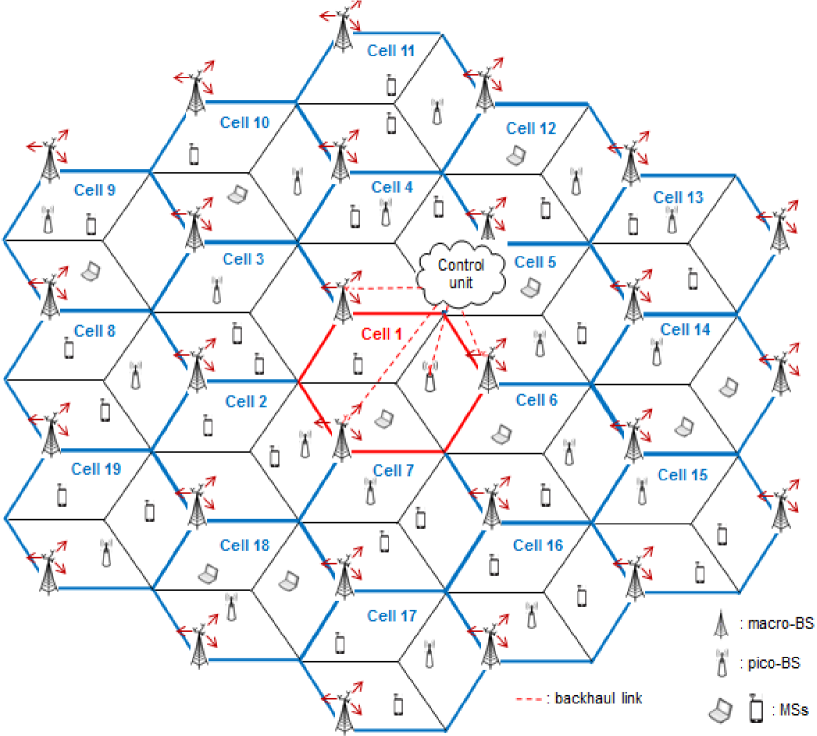
Figure 1: Two-dimensional hexagonal cellular layout with 19 macro hexagonal cells. Each macro BS has three sectorized antennas, while pico-BSs and MSs use omni-directional antennas. We are interested in the performance at macro cell 1 located at the center of the figure.

II System Model

We consider the two-dimensional hexagonal cellular layout with 19 macro cells shown in Fig. 1. We assume that each macro-base station (BS) uses three sectorized antennas, and each pico-BS and mobile station (MS) uses a single omni-directional antenna. In each macro-cell, $K$ MSs and $N$ pico-BSs are uniformly distributed. Fig. 1 illustrates an example with $K=2$ MSs and $N=1$ pico-BS.

In a C-RAN system, the baseband processing of the available macro- or pico/femto-BSs is migrated to control units, each of which manages a subset of BS antennas. For example, in Fig. 1, a control unit manages the three sectors of cell 1 and hence the corresponding sectorial antennas of the three relevant macro-BSs and the available pico-BS. We refer to a subset of BS antennas connected to the same control unit, and to the corresponding covered area, as a cluster.

Every $i$th BS is connected to the corresponding control unit via a backhaul link with capacity $C_{i}$ bps/Hz [3] where the normalization is done with respect to the bandwidth of the wireless uplink/downlink channels. For instance, if BS $i$ communicates with the corresponding control unit at a date rate of 100 Mbps and the wireless uplink/downlink channels have a 10 MHz bandwidth, the normalized backhaul capacity is given as $C_{i}=10$ bps/Hz.

According to the C-RAN principle, the data exchanged on the backhaul links between BSs and control units consists of compressed baseband signals [1]-[5]. Specifically, in the uplink, the baseband signal received by each BS is compressed and forwarded to the connected control unit, where decoding takes place. Instead, in the downlink, the baseband signals are produced and compressed by the control units, and then upconverted and transmitted by the BSs.

In the following, we detail the signal and channel model by focusing on one specific cluster, e.g., cell 1 in Fig. 1. For notational convenience, we index the BSs in the cluster as $1,2,\ldots,N_{B}$ and the MSs in the cluster as $1,2,\ldots,N_{M}$, and define the sets $\mathcal{N_{B}}=\{1,\ldots,N_{B}\}$ and $\mathcal{N_{M}}=\{1,\ldots,N_{M}\}$.

II-A Uplink Channel

The signal $y_{i}^{\mathrm{ul}}$ received by BS $i$ in the cluster under study in the uplink is given by

$$y_{i}^{\mathrm{ul}}=\mathbf{h}_{i}^{\mathrm{ul}\dagger}\mathbf{x^{\mathrm{ul}}}+z_{i}^{\mathrm{ul}},$$ (1)

where $\mathbf{x^{\mathrm{ul}}=}[x_{1}^{\mathrm{ul}}\cdots x_{N_{M}}^{\mathrm{ul}}]^{T}$ is the $n_{M}\times 1$ vector of symbols transmitted by all the $N_{M}$ MSs in the cluster, with $x_{k}^{\mathrm{ul}}$ being the symbol transmitted by MS $k$; the noise $z_{i}^{\mathrm{ul}}\sim\mathcal{CN}(0,\sigma_{z_{i}^{\mathrm{ul}}}^{2})$ models thermal noise and the interference signals arising from the other clusters; and the channel vector $\mathbf{h}_{i}^{\mathrm{ul}}\in\mathbb{C}^{N_{M}\times 1}$ from all the $N_{M}$ MSs in the cluster toward BS $i$ is given by $\mathbf{h}_{i}^{\mathrm{ul}}=[h_{i,1}^{\mathrm{ul}}\,\,h_{i,2}^{\mathrm{ul}}\,\,\cdots\,\,h_{i,N_{M}}^{\mathrm{ul}}]^{T}$ with $h_{i,k}^{\mathrm{ul}}$ denoting the uplink channel response from the $k$th MS and to the $i$th BS. The signal $x_{k}^{\mathrm{ul}}$ is subject to the per-MS power constraint, which is stated as $\mathbb{E}[|x_{k}^{\mathrm{ul}}|^{2}]\leq P_{M,k}$ for $k\in\mathcal{N_{M}}$.

II-B Downlink Channel

In the downlink, each MS $k$ in the cluster under study receives a signal given as

$$y_{k}^{\mathrm{dl}}=\mathbf{h}_{k}^{\mathrm{dl}\dagger}\mathbf{x}^{\mathrm{dl}}+z_{k}^{\mathrm{dl}},$$ (2)

where we have defined the aggregate transmit signal vector by all the $N_{B}$ BSs in the cluster as $\mathbf{x}^{\mathrm{dl}}=[x_{1}^{\mathrm{dl}},\ldots,x_{N_{B}}^{\mathrm{dl}}]^{T}$ with $x_{i}^{\mathrm{dl}}$ denoting the signal transmitted by the $i$th BS; the additive noise $z_{k}^{\mathrm{dl}}\sim\mathcal{CN}(0,\sigma_{z_{k}^{\mathrm{dl}}}^{2})$ accounts for thermal noise and interference from the other clusters; and the channel vector $\mathbf{h}_{k}^{\mathrm{dl}}\in\mathbb{C}^{N_{B}\times 1}$ from all the BSs in the cluster toward MS $k$ is given as $\mathbf{h}_{k}^{\mathrm{dl}}=[h_{k,1}^{\mathrm{dl}}\,\,h_{k,2}^{\mathrm{dl}}\,\,\cdots\,\,h_{k,N_{B}}^{\mathrm{dl}}]^{T}$ with $h_{k,i}^{\mathrm{dl}}$ denoting the downlink channel gain from BS $i$ to MS $k$. Finally, we have the per-BS power constraints $\mathbb{E}[|x_{i}^{\mathrm{dl}}|^{2}]\leq P_{B,i}$, for $i\in\mathcal{N_{B}}$.

For both uplink and downlink, the channel vectors $\{\mathbf{h}_{i}^{\mathrm{ul}}\}_{i\in\mathcal{N_{B}}}$ and $\{\mathbf{h}_{k}^{\mathrm{dl}}\}_{k\in\mathcal{N_{M}}}$ remain constant for the entire coding block duration and are known to the corresponding control unit. As discussed in Sec. I, the main goal of this paper is to provide a realistic evaluation of the advantages of the multiterminal backhaul compression strategies proposed in [9] for the uplink and in [11] for the donwlink. In the next two sections, we review these strategies.

III Multiterminal Compression for the Uplink of C-RAN

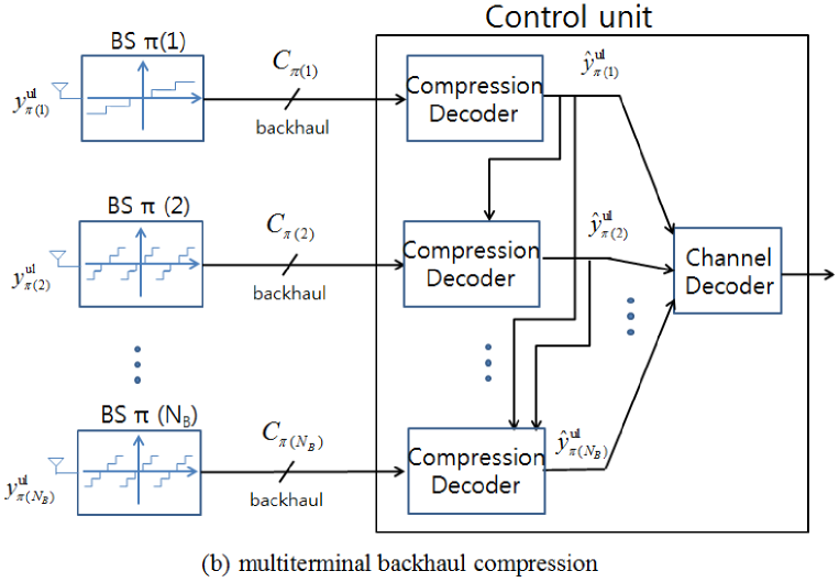
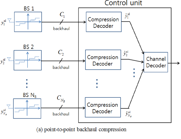
Figure 2: Backhaul compression and decompression for the uplink of C-RAN: (a) point-to-point compression; (b) multiterminal compression.

In the uplink of C-RAN, each MS $k$ within the cluster under study encodes its message $M_{k}$ to produce a transmitted signal $x_{k}^{\mathrm{ul}}$ for each channel use. This signal is taken from a conventional Gaussian codebook and is hence distributed as $x_{k}^{\mathrm{ul}}\sim\mathcal{CN}(0,P_{k})$ where $P_{k}$ satisfies the per-MS power constraint $P_{k}\leq P_{M,k}$. Note that, since the MSs cannot cooperate with each other, the transmitted signals $x_{k}^{\mathrm{ul}}$ are independent across the MS index $k$.

Each $i$th BS communicates with the control unit by providing the latter with a compressed version $\hat{y}_{i}^{\mathrm{ul}}$ of the received signal $y_{i}^{\mathrm{ul}}$. The control unit first decompresses the signals $\hat{y}_{i}^{\mathrm{ul}}$, $i\in\mathcal{N_{B}}$, and then, based on all signals $\hat{y}_{\mathcal{N_{B}}}^{\mathrm{ul}}$, decodes the MSs’ messages. Using standard rate-distortion considerations, we express the compressed signal $\hat{y}_{i}^{\mathrm{ul}}$ as

$$\hat{y}_{i}^{\mathrm{ul}}=y_{i}^{\mathrm{ul}}+q_{i}^{\mathrm{ul}},$$ (3)

where the quantization noise $q_{i}^{\mathrm{ul}}$ is independent of the signal $y_{i}^{\mathrm{ul}}$ and distributed as $q_{i}^{\mathrm{ul}}\sim\mathcal{CN}(0,\omega_{i}^{\mathrm{ul}})$.

Point-to-Point Backhaul Compression [14]: In a conventional system, the control unit decompresses the descriptions $\hat{y}_{\mathcal{N_{B}}}^{\mathrm{ul}}$ in parallel as shown in Fig. 2-(a). In this case, the signal $\hat{y}_{i}^{\mathrm{ul}}$ can be recovered at the control unit if the condition

$$I(y_{i}^{\mathrm{ul}};\hat{y}_{i}^{\mathrm{ul}}) =\log_{2}\left(\omega_{i}^{\mathrm{ul}}+\sigma_{y_{i}^{\mathrm{ul}}}^{2}\right)-\log_{2}\left(\omega_{i}^{\mathrm{ul}}\right)\leq C_{i}$$ (4)

is satisfied where $\sigma_{y_{i}^{\mathrm{ul}}}^{2}=\mathbf{h}_{i}^{\mathrm{ul}\dagger}\mathbf{\Sigma}_{\mathbf{x}^{\mathrm{ul}}}\mathbf{h}_{i}^{\mathrm{ul}}+\sigma_{z_{i}^{\mathrm{ul}}}^{2}$ with $\mathbf{\Sigma}_{\mathbf{x}^{\mathrm{ul}}}=\mathrm{diag}(\{P_{k}\}_{k\in\mathcal{N_{M}}})$ (see, e.g., [6, Ch. 3]).

Multiterminal Backhaul Compression [7]-[10]: Standard point-to-point compression does not leverage the statistical correlation among the signals $y_{i}^{\mathrm{ul}}$ received at different BSs. Based on this observation, distributed compression was proposed in [7] to utilize such correlation. Following [9][10], this can be done as follows. For a given ordering $\pi$ of the BS indices, the control unit decompresses in the order $\hat{y}_{\pi(1)}^{\mathrm{ul}},\hat{y}_{\pi(2)}^{\mathrm{ul}},\ldots,\hat{y}_{\pi(N_{B})}^{\mathrm{ul}}$ as shown in Fig. 2-(b). Therefore, when decompressing $\hat{y}_{\pi(i)}^{\mathrm{ul}}$, the control unit has already retrieved the signals $\hat{y}_{\pi(1)}^{\mathrm{ul}},\ldots,\hat{y}_{\pi(i-1)}^{\mathrm{ul}}$. These signals can be hence treated as side information available at the decoder, namely the control unit, but not to the encoder, namely BS $\pi(i)$. As a result, using the Wyner-Ziv theorem [6, Ch. 3], the descriptions $\hat{y}_{\pi(i)}^{\mathrm{ul}}$ for $i\in\mathcal{N_{B}}$ can be recovered at the control unit if the conditions

$$I(y_{\pi(i)}^{\mathrm{ul}};\hat{y}_{\pi(i)}^{\mathrm{ul}}|\hat{y}_{\{\pi(1),...,\pi(i-1)\}}^{\mathrm{ul}})= g_{\pi,i}^{\mathrm{ul}}(\mathbf{p},\mbox{\boldmath${\omega}$})$$ (5)

$$\triangleq \log_{2}\left(\omega_{\pi(i)}^{\mathrm{ul}}+\sigma_{y_{\pi(i)}^{\mathrm{ul}}|\hat{y}_{\{\pi(1),...,\pi(i-1)\}}^{\mathrm{ul}}}^{2}\right)-\log_{2}\left(\omega_{\pi(i)}^{\mathrm{ul}}\right)\leq C_{\pi(i)}$$

are satisfied, where we have defined vectors $\mathbf{p}=[P_{1},\ldots,P_{N_{M}}]$ and $\mbox{\boldmath${\omega}$}=[\omega_{1},\ldots,\omega_{N_{B}}]$, and the conditional variance $\sigma_{y_{\pi(i)}^{\mathrm{ul}}|\hat{y}_{\{\pi(1),...,\pi(i-1)\}}^{\mathrm{ul}}}^{2}$ is given by

$$\sigma_{y_{\pi(i)}^{\mathrm{ul}}|\hat{y}_{\{\pi(1),...,\pi(i-1)\}}^{\mathrm{ul}}}^{2}=\mathbf{h}_{\pi(i)}^{\mathrm{ul}\dagger}\mathbf{\Sigma}_{\mathbf{x}^{\mathrm{ul}}|\hat{y}_{\{\pi(1),...,\pi(i-1)\}}^{\mathrm{ul}}}\mathbf{h}_{\pi(i)}^{\mathrm{ul}}+\sigma_{z_{\pi(i)}^{\mathrm{ul}}}^{2},$$ (6)

with $\mathbf{\Sigma}_{\mathbf{x}^{\mathrm{ul}}|\hat{y}_{\{\pi(1),...,\pi(i-1)\}}^{\mathrm{ul}}}=\mathbf{\Sigma}_{\mathbf{x}^{\mathrm{ul}}}-\mathbf{\Sigma}_{\mathbf{x}^{\mathrm{ul}},\hat{y}_{\{\pi(1),...,\pi(i-1)\}}^{\mathrm{ul}}}\mathbf{\Sigma}_{\hat{y}_{\{\pi(1),...,\pi(i-1)\}}^{\mathrm{ul}}}^{-1}\mathbf{\Sigma}_{\mathbf{x}^{\mathrm{ul}},\hat{y}_{\{\pi(1),...,\pi(i-1)\}}^{\mathrm{ul}}}^{\dagger}$. The matrices $\mathbf{\Sigma}_{\mathbf{x}^{\mathrm{ul}},\hat{y}_{\{\pi(1),...,\pi(i-1)\}}^{\mathrm{ul}}}$ and $\mathbf{\Sigma}_{\hat{y}_{\{\pi(1),...,\pi(i-1)\}}^{\mathrm{ul}}}$ are given by

$$\mathbf{\Sigma}_{\mathbf{x}^{\mathrm{ul}},\hat{y}_{\{\pi(1),...,\pi(i-1)\}}^{\mathrm{ul}}}=\mathbf{\Sigma}_{\mathbf{x}^{\mathrm{ul}}}\mathbf{H}_{\pi,i-1}^{\mathrm{ul}\dagger},$$ (7)

$$\mathrm{and}\,\, \mathbf{\Sigma}_{\hat{y}_{\{\pi(1),...,\pi(i-1)\}}^{\mathrm{ul}}}=\mathbf{H}_{\pi,i-1}^{\mathrm{ul}}\mathbf{\Sigma}_{\mathbf{x}^{\mathrm{ul}}}\mathbf{H}_{\pi,i-1}^{\mathrm{ul}\dagger}+\mathrm{diag}\left(\{\sigma_{z_{\pi(j)}^{\mathrm{ul}}}^{2}+\omega_{\pi(j)}^{2}\}_{j=1}^{i-1}\right),$$ (8)

where we have defined the matrix $\mathbf{H}_{\pi,i-1}^{\mathrm{ul}}=[\mathbf{h}_{\pi(1)}^{\mathrm{ul}},\ldots,\mathbf{h}_{\pi(i-1)}^{\mathrm{ul}}]^{\dagger}$.

We assume that the control unit performs single-user decoding of the messages $\{M_{k}\}_{k\in\mathcal{N_{M}}}$ sent by MSs based on all the descriptions $\{\hat{y}_{i}^{\mathrm{ul}}\}_{i\in\mathcal{N_{B}}}$, so that each message $M_{k}$ is decoded by treating the interference signals $x_{j}^{\mathrm{ul}}$ for $j\neq k$ as noise (see [9] for the analysis with joint decoding of all MSs and [10] for successive interference cancellation). Under this assumption, the achievable rate $R_{k}$ for MS $k$ is given by

$$R_{k}^{\mathrm{ul}}= I(x_{k}^{\mathrm{ul}};\hat{y}_{\mathcal{N_{B}}}^{\mathrm{ul}})=f_{k}^{\mathrm{ul}}(\mathbf{p},\mbox{\boldmath${\omega}$})$$ (9)

$$\triangleq \log_{2}\det\left(\mathrm{diag}\left(\{\omega_{i}^{\mathrm{ul}}\}_{i\in\mathcal{N_{B}}}\right)+\mathbf{\Sigma}_{\mathbf{y}_{\mathcal{N_{B}}}^{\mathrm{ul}}}\right)-\log_{2}\det\left(\mathrm{diag}\left(\{\omega_{i}^{\mathrm{ul}}\}_{i\in\mathcal{N_{B}}}\right)+\mathbf{\Sigma}_{\mathbf{y}_{\mathcal{N_{B}}}^{\mathrm{ul}}|x_{k}^{\mathrm{ul}}}\right),$$

where the conditional covariance $\mathbf{\Sigma}_{\mathbf{y}_{\mathcal{N_{B}}}^{\mathrm{ul}}|x_{\mathcal{S}}^{\mathrm{ul}}}$ with $\mathcal{S}\subseteq\mathcal{N_{M}}$ is given as

$$\mathbf{\Sigma}_{\mathbf{y}_{\mathcal{N_{B}}}^{\mathrm{ul}}|x_{\mathcal{S}}^{\mathrm{ul}}}=\sum_{j\in\mathcal{N_{M}}\setminus\mathcal{S}}P_{j}\tilde{\mathbf{h}}_{j}^{\mathrm{ul}}\tilde{\mathbf{h}}_{j}^{\mathrm{ul}\dagger}+\mathrm{diag}\left(\{\sigma_{z_{i}^{\mathrm{ul}}}^{2}\}_{i\in\mathcal{N_{B}}}\right)$$ (10)

with $\tilde{\mathbf{h}}_{k}^{\mathrm{ul}}=[h_{1,k}^{\mathrm{ul}},h_{2,k}^{\mathrm{ul}},\ldots,h_{N_{B},k}^{\mathrm{ul}}]^{T}$.

We are interested in evaluating the performance of the standard proportional-fair scheduler. This scheduler, at each time slot, select the power allocation $\mathbf{p}$ and the quantization noise powers ${\omega}$ and the order $\pi$ so as to maximize the weighted sum-rate

$$u^{\mathrm{ul}}(\mathbf{p},\mbox{\boldmath${\omega}$})=\sum_{k\in\mathcal{N_{M}}}f_{k}^{\mathrm{ul}}(\mathbf{p},\mbox{\boldmath${\omega}$})/\bar{R}_{k}^{\alpha},$$ (11)

with $\alpha\geq 0$ being a fairness constant and $\bar{R}_{k}$ represents the average data rate of MS $k$ until the previous time slot (see, e.g., [15]). After each time slot, the rate $\bar{R}_{k}$ is updated as $\bar{R}_{k}\leftarrow\beta\bar{R}_{k}+(1-\beta)R_{k}^{\mathrm{ul}}$ where $\beta\in[0,1]$ is a forgetting factor. We recall that increasing the constant $\alpha$ encourages fairness among the MSs, while the objective function reduces to the sum-rate when $\alpha=0$. This problem is formulated as

$$\underset{\pi,\mathbf{p}\in\mathbb{R}_{+}^{N_{M}},\mbox{\boldmath${\omega}$}\in\mathbb{R}_{+}^{N_{B}}}{\mathrm{maximize}} u^{\mathrm{ul}}(\mathbf{p},\mbox{\boldmath${\omega}$})$$ (12a)

$$\mathrm{s.t.}\,\,\,\,\, g_{\pi,i}^{\mathrm{ul}}(\mathbf{p},\mbox{\boldmath${\omega}$})\leq C_{\pi(i)},\,\,\mathrm{for\,\,all}\,\,i\in\mathcal{N_{B}},$$ (12b)

$$P_{k}\leq P_{M,k},\,\,\mathrm{for\,\,all}\,\,k\in\mathcal{N_{M}}.$$ (12c)

To tackle the non-convex problem (12), we propose a separate design of the power control variables $\mathbf{p}$ and the compression noise powers ${\omega}$ for a fixed permutation $\pi$. Specifically, at Step 1, the power coefficients $\mathbf{p}$ are optimized assuming ideal backhaul links (i.e., $\mathbf{\omega}_{i}^{\mathrm{ul}}=0$ for $i\in\mathcal{N_{B}}$). This problem is stated as

$$\underset{\mathbf{p}\in\mathbb{R}_{+}^{N_{M}}}{\mathrm{maximize}} \,\,u^{\mathrm{ul}}(\mathbf{p},\mathbf{0})$$ (13)

$$\mathrm{s.t.}\,\,\,\,\, P_{k}\leq P_{M,k},\,\,\mathrm{for\,\,all}\,\,k\in\mathcal{N_{M}},$$

or, equivalently, in the epigraph form

$$\underset{R_{k},\mathbf{p}\in\mathbb{R}_{+}^{N_{M}}}{\mathrm{maximize}} \,\,\sum_{k\in\mathcal{N_{M}}}R_{k}/\bar{R}_{k}^{\alpha}$$ (14a)

$$\mathrm{s.t.}\,\,\,\,\, R_{k}\leq f_{k}^{\mathrm{ul}}(\mathbf{p},\mathbf{0}),\,\,\mathrm{for\,\,all}\,\,k\in\mathcal{N_{M}},$$ (14b)

$$P_{k}\leq P_{M,k},\,\,\mathrm{for\,\,all}\,\,k\in\mathcal{N_{M}}.$$ (14c)

Albeit still non-convex, it is seen that the problem (14) belongs to the class of different-of-convex (DC) problems (see, e.g., [16]). Thus, we can leverage the iterative majorization minimization (MM) algorithm, which is known to converge to a locally optimal point of (14) (see, e.g., [16, Sec. 1.3.3]). The MM algorithm solves a sequence of convex problems obtained by linearizing the non-convex constraints (14b). With the so-obtained power variables $\mathbf{p}$, at Step 2, we optimize the quantization noise powers ${\omega}$. It can be seen that the optimal quantization power $\omega_{\pi(i)}^{\mathrm{ul}}$, for fixed powers $\mathbf{p}$, is simply given by imposing equality in the backhaul constraint (12b), leading to

$$\omega_{\pi(i)}^{\mathrm{ul}}=\sigma_{y_{\pi(i)}^{\mathrm{ul}}|\hat{y}_{\{\pi(1),...,\pi(i-1)\}}^{\mathrm{ul}}}^{2}/(2^{C_{\pi(i)}}-1)$$ (15)

for $i\in\mathcal{N_{B}}$ with $\sigma_{y_{\pi(i)}^{\mathrm{ul}}|\hat{y}_{\{\pi(1),...,\pi(i-1)\}}^{\mathrm{ul}}}^{2}$ given in (6).

IV Multiterminal Compression for the Downlink of C-RAN

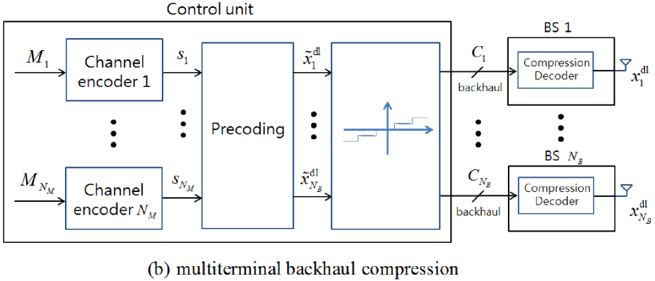
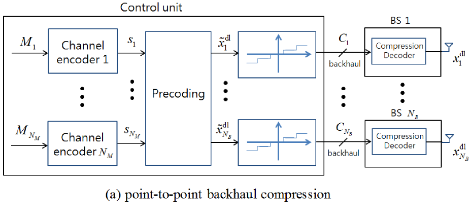
Figure 3: Backhaul compression and decompression for the downlink of C-RAN: (a) point-to-point compression; (b) multiterminal compression.

In the downlink of a C-RAN, the control unit first encodes each message $M_{k}$ for MS $k\in\mathcal{N_{M}}$ via a separate channel encoder, which produces a coded signal $s_{k}$ for each channel use. Each coded symbol $s_{k}$ is taken from a conventional Gaussian codebook and hence it is distributed as $s_{k}\sim\mathcal{CN}(0,1)$. The signals $\mathbf{s}=[s_{1},\ldots,s_{N_{M}}]$ are further processed by the control unit in two stages, namely precoding and compression.

1. Precoding: In order to allow for interference management both across the MSs and among the data streams for the same MS, the signals in vector $\mathbf{s}$ are linearly precoded via multiplication of a complex matrix $\mathbf{A}\in\mathbb{C}^{N_{B}\times N_{M}}$. The precoded data can be written as

$$\tilde{\mathbf{x}}^{\mathrm{dl}}=\mathbf{A}\mathbf{s},$$ (16)

where the matrix $\mathbf{A}$ can be factorized as $\mathbf{A}=[\mathbf{a}_{1}\,\cdots\,\mathbf{a}_{N_{M}}]$ with $\mathbf{a}_{k}\in\mathbb{C}^{N_{B}\times 1}$ denoting the precoding vector corresponding to MS $k$. The precoded data $\tilde{\mathbf{x}}^{\mathrm{dl}}$ can be written as $\tilde{\mathbf{x}}^{\mathrm{dl}}=[\tilde{x}_{1}^{\mathrm{dl}},\ldots,\tilde{x}_{N_{B}}^{\mathrm{dl}}]^{T}$, where the signal $\tilde{x}_{i}^{\mathrm{dl}}$ is the precoded signal corresponding to the $i$th BS and is given as $\tilde{x}_{i}^{\mathrm{dl}}=\mathbf{e}_{i}^{\dagger}\mathbf{A}\mathbf{s}$ with the vector $\mathbf{e}_{i}\in\mathbb{C}^{N_{B}\times 1}$ having all zero elements except for the $i$th element that contains 1.

2-(a). Point-to-Point Backhaul Compression [17]: Each precoded data stream $\tilde{x}_{i}^{\mathrm{dl}}$ for $i\in\mathcal{N_{B}}$ must be compressed in order to allow the control unit to deliver it to the $i$th BS through the backhaul link of capacity $C_{i}$ bps/Hz. Each $i$th BS then simply forwards the compressed signal $x_{i}^{\mathrm{dl}}$ obtained from the control unit. Using standard rate-distortion considerations, we adopt a Gaussian test channel to model the effect of compression on the backhaul link. In particular, we write the compressed signals $x_{i}^{\mathrm{dl}}$ to be transmitted by BS $i$ as

$$x_{i}^{\mathrm{dl}} =\tilde{x}_{i}^{\mathrm{dl}}+q_{i}^{\mathrm{dl}},$$ (17)

where the compression noise $q_{i}^{\mathrm{dl}}$ is modeled as a complex Gaussian noise. With conventional backhaul compression, as shown in Fig. 3-(a), the signal $\tilde{x}_{i}^{\mathrm{dl}}$ corresponding to different BSs are compressed separately, which leads to independent quantization noises $q_{i}^{\mathrm{dl}}$. Similar to the uplink, the compressed signal (17) can be transmitted to the $i$th BS if the condition

$$I\left(\tilde{\mathbf{x}}_{i};\mathbf{x}_{i}\right)=\log_{2}\left(\mathbf{e}_{i}^{\dagger}\mathbf{A}\mathbf{A}^{\dagger}\mathbf{e}_{i}+\omega_{i,i}^{\mathrm{dl}}\right)-\log_{2}\left(\omega_{i,i}^{\mathrm{dl}}\right)\leq C_{i}$$ (18)

is satisfied.

We now discuss the multiterminal backhaul compression strategies proposed in [11], and illustrated in Fig. 3-(b).

2-(b). Multiterminal Backhaul Compression [11]: The main idea of the multiterminal backhaul compression for the downlink is to control the effect of the additive quantization noises at the MSs by designing their correlation across the BSs within the cluster. This is made possible by multivariate compression [6, Ch. 7], which requires joint compression of all signals as in Fig. 3-(b). A successive compression implementation, which is dual to the successive decompression implementation of distributed source coding shown in Fig. 2-(b) for the uplink, is detailed in [11, Sec. IV-D].

To elaborate, we write the vector $\mathbf{x}^{\mathrm{dl}}=[x_{1}^{\mathrm{dl}},\ldots,x_{N_{B}}^{\mathrm{dl}}]^{T}$ of compressed signals for all the BSs as

$$\mathbf{x}^{\mathrm{dl}}=\mathbf{A}\mathbf{s}+\mathbf{q}^{\mathrm{dl}}.$$ (19)

In (19), the compression noise $\mathbf{q}^{\mathrm{dl}}=[q_{1}^{\mathrm{dl}},\ldots,q_{N_{B}}^{\mathrm{dl}}]^{T}$ is modeled as a complex Gaussian vector $\mathbf{q}^{\mathrm{dl}}\sim\mathcal{CN}(\mathbf{0},\mathbf{\Omega}^{\mathrm{dl}})$, where the covariance matrix $\mathbf{\Omega}^{\mathrm{dl}}$ consists of elements $\omega_{i,j}^{\mathrm{dl}}=\mathbb{E}[q_{i}^{\mathrm{dl}}q_{j}^{\mathrm{dl}\dagger}]$ defining the correlation between the quantization noises of BS $i$ and BS $j$.

Using the multivariate compression lemma in [6, Ch. 9], reference [11] shows that the signals $x_{1}^{\mathrm{dl}},\ldots,x_{N_{B}}^{\mathrm{dl}}$ obtained via the test channel (19) can be reliably transferred to the BSs on the backhaul links if the condition

$$g_{\mathcal{S}}^{\mathrm{dl}}\left(\mathbf{A},\mathbf{\Omega}^{\mathrm{dl}}\right) \triangleq\sum_{i\in\mathcal{S}}h\left(x_{i}^{\mathrm{dl}}\right)-h\left(x_{\mathcal{S}}^{\mathrm{dl}}|\tilde{\mathbf{x}}^{\mathrm{dl}}\right)$$ (20)

$$=\sum_{i\in\mathcal{S}}\log_{2}\left(\mathbf{e}_{i}^{\dagger}\mathbf{A}\mathbf{A}^{\dagger}\mathbf{e}_{i}+\omega_{i,i}^{\mathrm{dl}}\right)-\log_{2}\det\left(\mathbf{E}_{\mathcal{S}}^{\dagger}\mathbf{\Omega}^{\mathrm{dl}}\mathbf{E}_{\mathcal{S}}\right)\leq\sum_{i\in\mathcal{S}}C_{i}$$

is satisfied for all subsets $\mathcal{S}\subseteq\mathcal{N_{B}}$, where the matrix $\mathbf{E}_{\mathcal{S}}$ is obtained by stacking the vectors $\mathbf{e}_{i}$ for $i\in\mathcal{S}$ horizontally. We observe that the inequalities (18) for standard point-to-point compression are obtained by substituting $\omega_{i,j}^{\mathrm{dl}}=0$ into (20).

With the described precoding and compression operations and assuming that the interference signals are treated as noise signals at MSs, the achievable rate $R_{k}$ for MS $k$ is computed as

$$R_{k} =I\left(s_{k};y_{k}^{\mathrm{dl}}\right)=f_{k}^{\mathrm{dl}}\left(\mathbf{A},\mathbf{\Omega}^{\mathrm{dl}}\right)$$ (21)

$$\triangleq\log_{2}\left(\sigma_{z_{k}^{\mathrm{dl}}}^{2}+\mathbf{h}_{k}^{\mathrm{dl}\dagger}\left(\mathbf{A}\mathbf{A}^{\dagger}+\mathbf{\Omega}^{\mathrm{dl}}\right)\mathbf{h}_{k}^{\mathrm{dl}}\right)-\log_{2}\left(\sigma_{z_{k}^{\mathrm{dl}}}^{2}+\mathbf{h}_{k}^{\mathrm{dl}\dagger}\left(\sum_{l\in\mathcal{N_{M}}\setminus\{k\}}\mathbf{a}_{l}\mathbf{a}_{l}^{\dagger}+\mathbf{\Omega}^{\mathrm{dl}}\right)\mathbf{h}_{k}^{\mathrm{dl}}\right).$$

Similar to the uplink, our goal is to implement the proportional fairness scheduler, which requires to optimize the weighted sum-rate over the precoding matrix $\mathbf{A}$ and the quantization covariance matrix $\mathbf{\mathbf{\Omega}}^{\mathrm{dl}}$, subject to the backhaul constraints (20) and the per-BS power constraints $P_{B,i}$. The weighted sum-rate $u^{\mathrm{dl}}(\mathbf{A},\mathbf{\Omega}^{\mathrm{dl}})$ is defined as in Sec. III. This problem is formulated as

$$\underset{\mathbf{A},\,\mathbf{\Omega}^{\mathrm{dl}}\succeq\mathbf{0}}{\mathrm{maximize}} \,\,u^{\mathrm{dl}}(\mathbf{A},\mathbf{\Omega}^{\mathrm{dl}})$$ (22a)

$$\mathrm{s.t.}\,\,\,\,\,\,\,\,\, g_{\mathcal{S}}^{\mathrm{dl}}\left(\mathbf{A},\mathbf{\Omega}^{\mathrm{dl}}\right)\leq\sum_{i\in\mathcal{S}}C_{i},\,\,\mathrm{for\,\,all}\,\,\mathcal{S}\subseteq\mathcal{N_{B}},$$ (22b)

$$\mathbf{e}_{i}^{\dagger}\mathbf{A}\mathbf{A}^{\dagger}\mathbf{e}_{i}+\omega_{i,i}^{\mathrm{dl}}\leq P_{B,i},\,\,\mathrm{for\,\,all}\,\,i\in\mathcal{N_{B}}.$$ (22c)

A stationary point of problem (22) can be found, as for (13), by applying the MM algorithm on its epigraph form. The detailed algorithm can be derived similar to [11, Sec. V-A].

V Performance Evaluation

In this section, we discuss the performance advantages of multiterminal backhaul compression for the uplink and downlink of C-RAN systems on a standard cellular model based on [12]. We focus on the performance evaluation in macro-cell 1 in Fig. 1, which is served by the three sectorized antennas from the corresponding macro-BSs and by $N$ pico-BSs. A control unit is connected to all BS antennas that serve cell 1 as in Fig. 1, which is to be hence considered as a cluster. The backhaul links to each macro-BS antenna and to each pico-BS have the capacities of $C_{\mathrm{macro}}$ and $C_{\mathrm{pico}}$ bps/Hz, respectively. All interference signals from other macro-cells, denoted by cell 2, cell 3,$\ldots$, cell 19, are treated as independent noise signals. We used the system parameters suggested in [12] and summarized in Table I, and adopted the LTE rate model proposed in [18, Annex A]. We assume that the fairness is measured during $T$ time slots in which the locations of pico-BSs and MSs are fixed and small-scale fading channels change independently from slot to slot.

Parameters	Assumptions
System bandwidth	10 MHz
Path-loss (macro-BS)	$\mathrm{PL}\,(\mathrm{dB})=128.1+37.6\log_{10}R$, $R$: distance in kilometers
Path-loss (pico-BS)	$\mathrm{PL}\,(\mathrm{dB})=38+30\log_{10}R$, $R$: distance in meters
Antenna pattern for sectorized macro-BS antennas	$A(\theta)=-\min\left[12(\theta/\theta_{3\mathrm{dB}})^{2},A_{m}\right]$, $\theta_{3\mathrm{dB}}=65\textdegree$, $A_{m}=20\,\mathrm{dB}$
Lognormal shadowing (macro-BS)	10 dB standard deviation
Lognormal shadowing (pico-BS)	6 dB standard deviation
Antenna gain after cable loss (macro-BS)	15 dBi
Antenna gain after cable loss (pico-BS and MS)	0 dBi
Noise figure	5 dB (macro-BS), 6 dB (pico-BS), 9 dB (MS)
Transmit power	46 dBm (macro-BS), 24 dBm (pico-BS), 23 dBm (MS)

Table I: Summary of the system parameters used for simulation.

Figure 4: Frequency reuse pattern proposed in [19, Sec. VI] with reuse factor $F=1/3$ .

As shown in [19], with frequency reuse factor $F=1$, the advantages of intra-cluster cooperation are masked by the effects of the interference coming from the adjacent clusters. Thus, we consider the frequency reuse pattern with $F=1/3$ proposed in [19] in which the available bandwidth is partitioned into three bands $B_{1}$, $B_{2}$ and $B_{3}$, which are allocated so as to minimize the resulting inter-cluster interference as illustrated in Fig. 4. As a result, cell 1 of interest suffers from the interference signals only from cells (8,10,12,14,16,18).

V-A Uplink

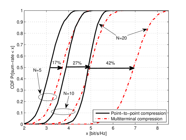
In this subsection, we examine the advantage of the multiterminal compression scheme based on distributed source coding reviewed in Sec. III for the uplink of the C-RAN described above. In Fig. 5, the CDF of the sum-rate is plotted with $K=5$ MSs, $(C_{\mathrm{macro}},C_{\mathrm{pico}})=(3,1)$ bps/Hz and $\alpha=0$. For the order $\pi$ on the BS, we assume that the control unit first retrieves the signals compressed at the macro-BSs and then decompresses the signals received from the pico-BSs. It is observed that, as compared to standard point-to-point compression, multiterminal compression provides performance gains of 17%, 27% and 42% for $N=5$, $10$ and $20$ pico-BSs, respectively, in terms of the 50%-ile sum-rate. Thus, the performance gain of the multiterminal compression is most pronounced when a large number of pico-BSs are located in the same cluster. This suggests that a sophisticated design of backhaul compression provides relevant gain if many radio units are concentrated in given areas.

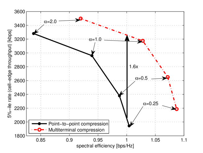
In Fig. 6, we plot the cell-edge throughput, i.e., the 5%-ile rate, versus the average spectral efficiency. The curve is obtained by varying the fairness constant $\alpha$ in the utility function (11) (see, e.g., [14, Fig. 5]). We fix $N=3$ pico-BSs, $K=5$ MSs, $(C_{\mathrm{macro}},C_{\mathrm{pico}})=(9,3)$ bps/Hz, $T=10$ and $\beta=0.5$. As we increase the constant $\alpha$, the 5%-ile rate increases due to the enhanced fairness among the MSs. We observe that spectral efficiencies larger than 1.01 bps/Hz are not achievable with point-to-point compression, while they can be obtained with multiterminal compression. Moreover, it is seen that multiterminal compression provides 1.6x gain in terms of cell-edge throughput for spectral efficiency of 2.9 bps/Hz.

Figure 5: CDF of the sum-rate in the uplink C-RAN with parameters as in [12, Tables 5.3.3-1, 5.3.4-1], $K=5$ MSs, $(C_{\mathrm{macro}},C_{\mathrm{pico}})=(3,1)$ bps/Hz and $\alpha=0$.

Figure 6: Cell-edge throughput, i.e., 5%-ile rate, versus the average spectral efficiency for various fairness constants $\alpha$ in the uplink C-RAN with $N=3$ pico-BSs, $K=5$ MSs, $(C_{\mathrm{macro}},C_{\mathrm{pico}})=(9,3)$ bps/Hz, $T=10$ and $\beta=0.5$.

V-B Downlink

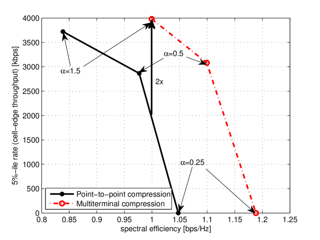
In this subsection, we turn to the advantage of the multiterminal compression technique as described in Sec. IV for the downlink. Fig. 7 plots the cell-edge throughput versus the average spectral efficiency for $N=3$ pico-BSs, $K=5$ MSs, $(C_{\mathrm{macro}},C_{\mathrm{pico}})=(9,3)$ bps/Hz, $T=10$ and $\beta=0.5$. As for the uplink, it is seen that spectral efficiencies larger than 1.05 bps/Hz are not achievable with point-to-point compression, while they can be obtained with multiterminal compression. Specifically, multiterminal compression provides about 2x gain in terms of cell-edge throughput for spectral efficiency of 1 bps/Hz.

Figure 7: Cell-edge throughput, i.e., 5%-ile rate, versus the average spectral efficiency for various fairness constants $\alpha$ in the downlink C-RAN with $N=1$ pico-BS, $K=4$ MSs, $(C_{\mathrm{macro}},C_{\mathrm{pico}})=(3,1)$ bps/Hz, $T=5$ and $\beta=0.5$.

VI Conclusion

In this work, we have studied the advantage of multiterminal backhaul compression techniques over standard point-to-point compression for the uplink and downlink of cloud radio access networks. The extensive simulations are based on standard cellular models and the results focused on performance metrics such as sum-rate, proportional-fairness utility and cell-edge throughput. As an example, we observed that multiterminal compression techniques provide performance gains of more than 60% for both the uplink and the downlink in terms of the cell-edge throughput.

References

• [1] J. Segel and M. Weldon, "Lightradio portfolio-technical overview," Technology White Paper 1, Alcatel-Lucent.
• [2] China Mobile, "C-RAN: the road towards green RAN," White Paper, ver. 2.5, China Mobile Research Institute, Oct. 2011.
• [3] T. Biermann, L. Scalia, C. Choi, W. Kellerer and H. Karl, "How backhaul networks influence the feasibility of coordinated multipoint in cellular networks," IEEE Comm. Mag., vol. 51, no. 8, pp. 168-176, Aug. 2013.
• [4] Ericsson AB, Huawei Technologies, NEC Corporation, Alcatel Lucent and Nokia Siemens Networks, "Common public radio interface (CPRI); interface specification," CPRI specification v5.0, Sep. 2011.
• [5] Integrated Device Technology, Inc., "Front-haul compression for emerging C-RAN and small cell networks," Apr. 2013.
• [6] A. E. Gamal and Y.-H. Kim, Network information theory, Cambridge University Press, 2011.
• [7] A. Sanderovich, O. Somekh, H. V. Poor and S. Shamai (Shitz), "Uplink macro diversity of limited backhaul cellular network," IEEE Trans. Inf. Theory, vol. 55, no. 8, pp. 3457-3478, Aug. 2009.
• [8] A. del Coso and S. Simoens, "Distributed compression for MIMO coordinated networks with a backhaul constraint," IEEE Trans. Wireless Comm., vol. 8, no. 9, pp. 4698-4709, Sep. 2009.
• [9] S.-H. Park, O. Simeone, O. Sahin and S. Shamai (Shitz), "Robust and efficient distributed compression for cloud radio access networks," IEEE Trans. Veh. Technology, vol. 62, no. 2, pp. 692-703, Feb. 2013.
• [10] L. Zhou and W. Yu, "Uplink multicell processing with limited backhaul via successive interference cancellation," in IEEE Global Comm. Conf. (Globecom 2012), Anaheim, CA, Dec. 2012.
• [11] S.-H. Park, O. Simeone, O. Sahin and S. Shamai (Shitz), "Joint precoding and multivariate backhaul compression for the downlink of cloud radio access networks," IEEE Trans. Sig. Processing, vol. 61, no. 22, pp. 5646-5658, Nov. 2013.
• [12] 3GPP TR 36.931 ver. 9.0.0 Rel. 9, May 2011.
• [13] S.-H. Park, O. Simeone, O. Sahin and S. Shamai (Shitz), "Joint decompression and decoding for cloud radio access networks," IEEE Sig. Processing Letters, vol. 20, no. 5, pp. 503-506, May 2013.
• [14] R. Irmer, H. Droste, P. Marsch, M. Grieger, G. Fettweis, S. Brueck, H.-P. Mayer, L. Thiele and V. Jungnickel, "Coordinated multipoint: concepts, performance, and field trial results," IEEE Comm. Mag., vol. 49, no. 2, pp. 102-111, Feb. 2011.
• [15] P. Viswanth, D. Tse and R. Laroia, "Opportunistic beamforming using dumb antennas," IEEE Trans. Inf. Theory, vol. 48, no. 6, pp. 1277-1294, Jun. 2002.
• [16] A. Beck and M. Teboulle, "Gradient-based algorithms with applications to signal recovery problems," in Convex Optimization in Signal Processing and Communications, Y. Eldar and D. Palomar, eds., pp. 42-88, Cambridge University Press. 2010.
• [17] O. Simeone, O. Somekh, H. V. Poor and S. Shamai (Shitz), "Downlink multicell processing with limited-backhaul capacity," EURASIP J. Adv. Sig. Proc., 2009.
• [18] 3GPP TR 36.942 ver. 8.1.0 Rel. 8, Jan. 2009.
• [19] L.-C. Wang and C.-J. Yeh, "3-cell network MIMO architectures with sectorization and fractional frequency reuse," IEEE J. Sel. Areas Comm., vol. 29, no. 6, pp. 1185-1199, Jun. 2011.