$Q^{2}$-evolution of the electric and magnetic polarizabilities of the proton

Abstract

The generalized Baldin sum rule at finite four-momentum transfer $Q^{2}$ is evaluated utilizing a structure function parameterization fit to recent experimental data. The most recent measurements on $F_{1}$ from Hall C at Jlab, as well as the $F_{2}$ structure function data from Hall B at Jlab and SLAC, were used in constructing our parameterization. We find that at $Q^{2}$ below 1 GeV² the dominant contribution to the electric and magnetic polarizabilities of the nucleon comes from the resonance region.

I Introduction

Understanding the internal structure of strongly interacting particles is one of the major goals of low-energy QCD. The study of the response of baryons to an external electromagnetic field via the multipole excitation mechanism provides direct access to the internal structure.

The parameters to describe that response are electric, magnetic, and spin-dependent polarizabilities. The polarizability is an elementary structure constant that is related to the deformation and stiffness of the baryon. Furthermore, the physical content of the polarizabilities is an effective multipole interaction for the coupling of the electric and magnetic fields of the photon with the internal structure of the baryon Babusci1 ; Holstein .

Evaluation of the electric $(\alpha)$ and magnetic $(\beta)$ polarizabilities of the nucleon has attracted much attention, both phenomenological and theoretical. The $Q^{2}$-dependence of the polarizabilities gives information on the polarization density in the nucleon. The $Q^{2}$-evolution of the sum of both polarizabilities can be determined through the generalized Baldin sum rule Drechsel , namely

$${\ \alpha}(Q^{2})+{\ \beta}(Q^{2})=\frac{8\,\alpha_{\rm em}\,M}{Q^{4}}\int_{0}^{x_{\pi}}\!x\,F_{1}(x,Q^{2})\,dx,$$ (1)

where $Q^{2}$ is four-momentum transfer squared, $\alpha_{\rm em}$ is the fine structure constant, $M$ stands for the nucleon mass, and $F_{1}$ is the nucleon structure function. Here $x$ is the Bjorken scaling variable,

$$x=\frac{Q^{2}}{W^{2}-M^{2}+Q^{2}},$$ (2)

where $W$ is the invariant mass of the final state, and $x_{\pi}$ corresponds to pion threshold. This implies that $F_{1}$ should be taken up to an infinite energy. Indeed it is necessary to use quite reliable models for the $W$-dependence as well as $Q^{2}$-dependence of the structure function in order to reduce the uncertainty of the sum rule evaluation.

Equation (1) provides information about the $Q^{2}$-evolution of the polarizabilities. An evaluation of the $Q^{2}$-dependence of the sum of electric and magnetic polarizabilities was done in 2006 by Liang et al. Liang1 . There was not much data on the $F_{1}$ structure function in the relevant kinematic region at that time. At high energies the SLAC Rosenbluth data Whitlow were used. In the resonance region the E94-110 measurements Liang2 ; Liang3 in Hall C at Jefferson Laboratory (JLab) from 2004 were used.

Up to now this evaluation of the $Q^{2}$-dependence of polarizabilities stands as the present “state of the art”. However, in 2013 an updated version of the E94-110 measurement appeared Liang4 . This has motivated us to reexamine the generalized Baldin sum rule.

At $Q^{2}=0$ the sum of electric and magnetic polarizabilities of the nucleon can be related to the unpolarized photo-absorption cross section $\sigma_{\gamma N\to X}$ as

$${\alpha}+{\beta}=\frac{1}{2\pi^{2}}\int_{\nu_{\pi}}^{\infty}\frac{\sigma_{\gamma N\to X}(\nu)}{\nu^{2}}d\nu,$$ (3)

where $\nu$ is the photon energy and $\nu_{\pi}$ is pion photo-production threshold. It is clear that at $Q^{2}=0$ Eq. (1) converges to Eq. (3), since

$$x=\frac{Q^{2}}{2M\nu}.$$ (4)

Indeed, Eq. (3) is the original formulation of the Baldin sum rule Baldin ; Lapidus .

The evaluation of the Baldin sum rule requires knowledge of the energy-dependence of $\sigma_{\gamma N\to X}(\nu)$ up to $\nu\to\infty$. However, as the integral is weighted by $1/\nu^{2}$, the contribution at low energies dominates the integral.

The sum of the polarizabilites for the proton was evaluated by Damashek and Gilman Damashek in 1970, and amounts to

$${\alpha}+{\beta}=(14.2\pm 0.3)\times 10^{-4}\,{\rm fm^{3}}.$$ (5)

A more recent calculation of Eq. (3) was done by Babusci et al. Babusci , with the result

$${\ \alpha}+{\ \beta}=(13.69\pm 0.14)\times 10^{-4}\,{\rm fm^{3}}.$$ (6)

The current PDG PDG averaged experimental values for electric and magnetic polarizabilities for proton are

$$\alpha = (12.0\pm 0.6)\times 10^{-4}\,{\rm fm^{3}},$$ (7a)

$$\beta = (1.9\pm 0.5)\times 10^{-4}\,{\rm fm^{3}}.$$ (7b)

Finally, a Chiral Perturbation Theory calculation Bernard predicts

$${\alpha}+{\beta}=(14.0\pm 4.1)\times 10^{-4}\,{\rm fm^{3}}$$ (8)

for the proton. An evaluation of the generalized polarizabilities at low $Q^{2}$ was considered by Hemmert et al. Hemmert .

A review of nucleon polarizabilities at $Q^{2}=0$ extracted from experimental data, as well as given by theoretical calculation, can be found in Ref. Babusci1 . A more recent review within the effective field theory approach can be found in Ref. Griesshammer . The polarizabilities at $Q^{2}=0$ provide a lower limit for the $Q^{2}$-dependence of the generalized Baldin sum rule.

Here we calculate the generalized Baldin sum rule, aiming to obtain the $Q^{2}$-dependence of the sum of generalized electric and magnetic proton polarizabilities. As a corollary, we obtain a convenient parameterization of the $F_{1}$ structure function from recent experimental data which is valid in the low-$Q^{2}$, low $W$ kinematic region.

The most recent results Liang4 for the $F_{1}$ structure function measured at Jlab Hall C were used for the contribution in the resonance region. Furthermore, we adopted the results on the $F_{2}$ structure function in the resonance region obtained at JLab. For that we apply the relation between $F_{2}$ and $F_{1}$ given by the ratio of longitudinal to transverse cross sections. That procedure provides us reasonable confidence in constructing the parameterization of the structure functions.

At energies above the resonance region we adopt the Regge approach. It is shown here that the Regge results are in good agreement with MRST leading twist fit MRST ; MSTW at $Q^{2}>1$ GeV². Note that the MRST parton distribution function is not provided for $Q^{2}<1$ GeV².

The paper is organized as follows. In Sec. II we show the details of our parameterization of the structure functions, and compare it with experimental results. The evaluation of the generalized Baldin sum rules is given in Sec. III. The paper ends with a summary.

II The parameterization

For the $F_{1}$ structure function we use the parameterization developed in Ref. Sibirtsev . The parameters of that model were obtained from the fit of experimental results for the $F_{2}$ structure function measured at JLab Liang3 ; Osipenko ; Niculascu ; Malace , as well as obtained at SLAC Whitlow1 . The structure functions $F_{1}$ and $F_{2}$ are related through the ratio of the longitudinal $\sigma_{L}$ to transverse $\sigma_{T}$ virtual photon cross sections as

$$R=\frac{\sigma_{L}}{\sigma_{T}}=\frac{F_{2}}{2xF_{1}}\left[1+\frac{4M^{2}x^{2}}{Q^{2}}\right]-1.$$ (9)

Figure 1: (Color online). The ratio of the longitudinal $\sigma_{L}$ to transverse $\sigma_{T}$ virtual photon cross sections as a function of energy $W$ shown for different $Q^{2}$. The circles are the results Liang4 from Jlab Hall C. The squares are the the results from SLAC Whitlow . Solid lines are our parameterization given by Eq. (10). Dashed lines show the parameterization from Ref. Ricco .

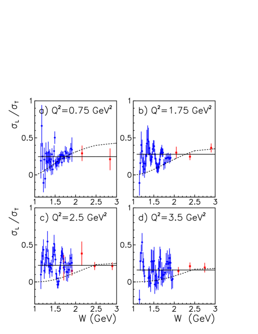
Figure 1 shows the experimental results for the ratio. The circles indicate the data Liang4 from Jlab Hall C, while the squares are the data from SLAC Whitlow . The ratio is shown for different $Q^{2}$. Here solid lines are our parameterization, given as

$$R=0.014\,Q^{2}\,\left[\exp(-0.07\,Q^{2})+41\,\exp(-0.8\,Q^{2})\right],$$ (10)

with $Q^{2}$ in units of GeV².

Actually the parameters of Eq. (10) were obtained from a fit of the experimental results shown in Fig. 1. Since the data at $W<2$ GeV are given with quite large statistical and experimental errors, we were not able to fit the fine structure of the ratio in the resonance region. Equation (10) provides a correct limit at $Q^{2}=0$ (i.e. $R=0$), since at the real photon point $\sigma_{L}=0$. Equation (10) was used to obtain the parameterization for the $F_{1}$ structure function from that given Sibirtsev for $F_{2}$.

Now we give the details of the $F_{2}$ parameterization, since these were not published in Ref. Sibirtsev . We did consider two regions with respect to energy $W$, namely the resonance and DIS regions.

At $W<1.9$ GeV we use the isobar model following the analyses of Refs. Cone ; Stein ; Brasse . The contributions from four resonances, namely $P33(1232)$, $D13(1520)$, $F15(1680)$ and $F37(1950)$, were considered. The resonance properties adopted in our analysis are listed in Table 1. Note that the masses and widths of the resonances were not taken from PDG PDG , but were obtained from the fit of experimental results for the $F_{2}$ structure function.

Table 1: Resonance parameters used in our isobar model.

Res.	$M_{R}$ (GeV)	$\Gamma_{R}$ (GeV)	$l$	$x_{R}$	$b$ (GeV${}^{-2})$	$A_{R}$
$P33$	1.22	0.119	1	0.16	1.51	723.1
$D13$	1.52	0.127	2	0.35	1.32	214.6
$F15$	1.70	0.117	3	0.35	0.81	95.6
$F37$	1.90	0.28	3	0.35	1.11	68.2

The resonance construction was parameterized by a relativistic Breit-Wigner shape as

$$\sigma_{R}=\frac{A_{R}\,M_{R}^{2}\,\Gamma_{1}\,\Gamma_{2}\,G(Q^{2})}{(M_{R}^{2}-W^{2})^{2}+M_{R}^{2}\Gamma_{1}^{2}}\,\left(\frac{k_{R}}{k}\right)^{2},$$ (11)

and we account for the energy-dependence of the width, namely

$$\Gamma_{1}=\Gamma_{R}\left(\frac{q}{q_{R}}\right)^{2l+1}\left(\frac{q^{2}+x_{R}^{2}}{q_{R}^{2}+x_{R}^{2}}\right)^{l},$$ (12a)

$$\Gamma_{2}=\Gamma_{R}\left(\frac{q}{q_{R}}\right)^{2l}\left(\frac{k^{2}+x_{R}^{2}}{k_{R}^{2}+x_{R}^{2}}\right)^{l}.$$ (12b)

Furthermore

$$k=\frac{\lambda^{1/2}(W^{2},m_{N}^{2},Q^{2})}{2W},$$ (13a)

$$k_{R}=\frac{\lambda^{1/2}(M_{R}^{2},m_{N}^{2},Q^{2})}{2M_{R}},$$ (13b)

$$q=\frac{\lambda^{1/2}(W^{2},m_{N}^{2},m_{\pi}^{2})}{2W},$$ (13c)

$$q_{R}=\frac{\lambda^{1/2}(M_{R}^{2},m_{N}^{2},m_{\pi}^{2})}{2M_{R}},$$ (13d)

with the kinematical function $\lambda$ defined as

$$\lambda(x,y,z)=(x-y-z)^{2}-4yz.$$ (14)

We introduce form factors at the interaction vertices, parameterized by an overall exponential function as

$$G(Q^{2})=\exp(-bQ^{2}),$$ (15)

with cut off parameters $b$ listed in Table 1. The parameters were fit to data Sibirtsev on the $F_{2}$-structure function.

With respect to Ref. Christy , we do not consider $S11(1535)$, $S11(1650)$, and $P11(1440)$ resonances. We found that it is difficult to separate these resonances from others in performing the fit and keep the resonance properties (e.g. strength, width) as free parameters. Since our strategy was to describe the experimental results on the structure function, not to study baryons, this approach seems quite reasonable.

Moreover, in the resonance region we consider in addition the non-resonant background contribution $F_{2}^{\rm bg}$. It was parameterized as

$$F_{2}^{\rm bg} = c_{1}c_{2}{(1-x)^{1.5}\over x^{0.6}},$$ (16a)

$$c_{1} = 4\,\pi^{2}\,\alpha_{\rm em}{Q^{2}+a_{\nu}^{2}\over Q^{2}a_{\nu}^{2}(1-x)},$$ (16b)

$$c_{2} = 0.0037575+0.075834\,Q^{2}$$ (16c)

$$+\,0.024600\,Q^{4}-0.0099514\,Q^{6},$$

$$x = {Q^{2}\over 2(M+m_{\pi})a_{\nu}},$$ (16d)

$$a_{\nu} = {W^{2}+Q^{2}-(M+m_{\pi})^{2}\over 2(M+m_{\pi})}.$$ (16e)

Figure 2: (Color online). $F_{1}$ structure function in the resonance region ($W<2$ GeV) shown for different $Q^{2}$ values. The circles are the results Liang4 from JLab Hall C, while the squares are from SLAC Whitlow . The shaded (green) band represents the uncertainty on our fit. The triangles are the results from the parameterization given in Ref. Christy .

Figure 3: (Color online). $F_{1}$ structure function above the resonance region shown for different $Q^{2}$ values. The squares are from SLAC Whitlow . The shaded (green) band represents the uncertainty on our fit. The triangles are the results from the parameterization given in Ref. Christy . The dashed lines illustrate results from MRST MRST ; MSTW .

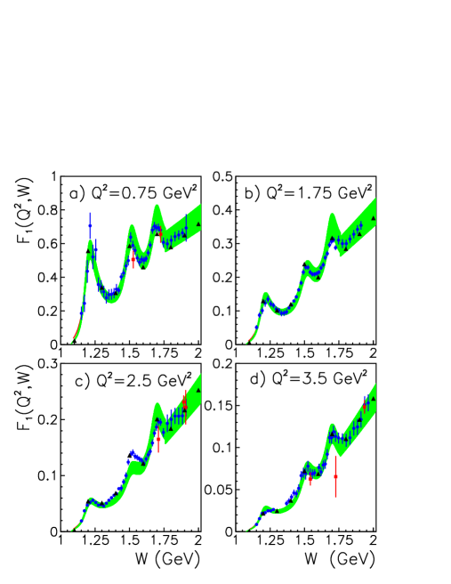
Figure 2 shows our calculations together with data for the $F_{1}$ structure function. The circles are experimental results from JLab Liang4 , and the squares indicate data from SLAC Whitlow . The shaded band represents the uncertainty in our fit. The triangles are results from the parameterization in Ref. Christy . It is clear that both parameterizations describe the data quite reasonably, although they are constructed in a different manner.

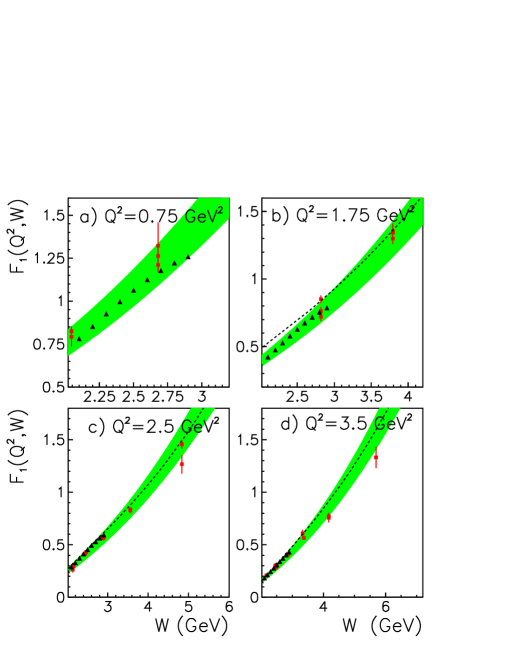
Above the resonance region we adopt the Regge model Capella ; Kaidalov ; Levin . The advantage of the Regge approach is that it can be used as well at low $Q^{2}$, where the MRST PDF description cannot be applied. The comparison of Regge results with MRST and data is given in Fig. 3. There is a reasonable agreement between MRST and Regge results, as well as describing the available data.

III Polarizabilities

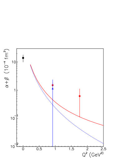
Now with the given parameterization for the $F_{1}$ structure function, we calculate the sum of electric and magnetic polarizabilities of the proton. Since the parameters of the model were fitted at $Q^{2}>0.225$ GeV², the results shown in Fig. 4 are for the relevant region. Here the dashed line indicates the result for energies $W<2$ GeV. The solid line is the result for the full range of energy. The square illustrates the prediction Bernard from ChPT.

We also show recent experimental results from Hall A given at $Q^{2}=0.92$ GeV² and 1.76 GeV² and evaluated by the dispersion relation approach. Unfortunately statistical and systematic errors of the data are too large, so it is not possible to make solid conclusions on the compatibility of our analysis and measurements. It appears that further precise experiments are required. Furthermore, at $Q^{2}<1$ GeV² the dominant contribution to polarizabilities comes from the resonance region.

Figure 4: (Color online). The sum of the electric and magnetic polarizabilites of the proton as a function of $Q^{2}$. The dashed line indicates the result for $W<2$ GeV, while the solid line show our calculation for the full range of energy. The square is the prediction Bernard given by Chiral Perturbation Theory at $Q^{2}=0$. Circles are the results from Hall A obtained with a dispersion relation approach and using data sets I-a and II halla . The triangle result is for data set I-b.

IV Summary

We evaluated the generalized Baldin sum rule using a structure function parameterization fit to experimental data. The most recent data on $F_{1}$ from Hall C at Jlab were used in our analysis. As well, we utilized the $F_{2}$ structure function data collected by the Hall B Collaboration at JLab and the $F_{2}/F_{1}$ ratio. SLAC results are also included in our analysis. We found that at $Q^{2}<1$ GeV² the dominant contribution to the sum of electric and magnetic polarizabilities comes from the resonance region, i.e. at energies $W<2$ GeV.

Further study is necessary at $Q^{2}<0.2$ GeV² to establish the transition to the real photon point. In the absence of experimental results in that region we could not develop a phenomenological model. It is important to construct a reliable parameterization for $F_{1}$ structure function if possible. We keep this study in progress.

We note that linear extrapolation of our results to the real photon point does not allow us to get polarizability at $Q^{2}=0$. That issue as well requires a more detailed study at low $Q^{2}$.